| Issue |
A&A
Volume 701, September 2025
|
|
|---|---|---|
| Article Number | A158 | |
| Number of page(s) | 18 | |
| Section | Extragalactic astronomy | |
| DOI | https://doi.org/10.1051/0004-6361/202555443 | |
| Published online | 09 September 2025 | |
The properties of X-ray-selected active galactic nuclei in protoclusters pinpointed by enormous Lyman alpha nebulae
1
Istituto Nazionale di Astrofisica (INAF) – Osservatorio di Astrofisica e Scienza dello Spazio (OAS), Via Gobetti 101, I-40129 Bologna, Italy
2
Max-Planck-Institut für Astrophysik, Karl-Schwarzschild-Str. 1, D-85748 Garching, Germany
3
Academia Sinica Institute of Astronomy and Astrophysics (ASIAA), 11F of Astronomy-Mathematics Building, AS/NTU, No. 1, Section 4, 12 Roosevelt Road, Taipei 106319, Taiwan
4
Dipartimento di Fisica e Astronomia (DIFA), Università di Bologna, Via Gobetti 93/2, I-40129 Bologna, Italy
5
Department of Astronomy and Astrophysics, UCO/Lick Observatory, University of California, Santa Cruz, 1156 High Street, Santa Cruz, CA 95064, USA
6
Dipartimento di Fisica “G. Occhialini”, Università degli Studi di Milano-Bicocca, Piazza della Scienza 3, 20126 Milano, Italy
7
INAF – Osservatorio Astrofisco di Arcetri, Largo E. Fermi 5, 50127 Firenze, Italy
8
Department of Physics and Astronomy, Clemson University, Kinard Lab of Physics, Clemson, SC 29634-0978, USA
9
Max-Planck-Institut für extraterrestrische Physik (MPE), Gießenbachstraße 1, 85748 Garching, Germany
⋆ Corresponding author.
Received:
8
May
2025
Accepted:
2
July
2025
Abstract
Context. Protoclusters of galaxies are overdense regions of the Universe characterized by large gas reservoirs. These environments make them ideal laboratories for investigating galaxy-AGN coevolution and the growth of SMBHs. Galaxies residing in such dense regions are expected to grow their SMBHs efficiently, resulting in a higher incidence of AGN than in the field. Some protoclusters exhibit extended Lyα nebulae in their central regions, indicating the presence of massive gas reservoirs, although their main powering mechanism remains debated.
Aims. We aim to investigate the AGN population, and AGN enhancement, in three protoclusters at 2.3 ≲ z ≲ 3.2, namely the Slug, Fabulous, and J0819, which host enormous (≈200 − 400 kpc) Lyα nebulae (ELANe). Additionally, we search for the presence of diffuse X-ray emission in the same regions of the Lyα nebulae to reveal multiphase gas in these protoclusters.
Methods. To identify AGN among the protocluster members, we used deep (texp ∼ 190 − 270 ks) Chandra observations and performed X-ray spectral analysis to derive the properties of those sources. We compared the AGN fraction and space density with those observed in other known protoclusters and from the field environment.
Results. Overall, we find 11 X-ray detected AGN in the three protoclusters (2, 5, and 4 in the Slug, Fabulous, and J0819, respectively). Each structure hosts a central, X-ray-powerful (log(LX/erg s−1)∼45 − 46) QSO, while the other X-ray sources are mostly moderately luminous (log(LX/erg s−1)∼44) and obscured, Compton-thin AGN. The fraction of AGN in our targets is comparable with estimates for other protoclusters and significantly higher than what is found for low-redshift clusters. We also find a significant enhancement (2–4 dex) in AGN density, relative to both the field and non-active galaxies in the protoclusters. Finally, we find no significant soft X-ray diffuse emission from the nebulae, thus ruling out gravitational heating as the main powering mechanism of the ELANe.
Key words: galaxies: active / galaxies: clusters: general / galaxies: evolution / galaxies: high-redshift / quasars: supermassive black holes / X-rays: galaxies
© The Authors 2025
 Open Access article, published by EDP Sciences, under the terms of the Creative Commons Attribution License (https://creativecommons.org/licenses/by/4.0), which permits unrestricted use, distribution, and reproduction in any medium, provided the original work is properly cited.
This article is published in open access under the Subscribe to Open model. This email address is being protected from spambots. You need JavaScript enabled to view it. to support open access publication.
1. Introduction
Supermassive black holes (SMBHs) play key roles in shaping the properties and evolution of the galaxies in which they are hosted (Magorrian et al. 1998; Ferrarese 2002; Kormendy & Ho 2013). This interplay is known as SMBH-galaxy coevolution (Kormendy & Ho 2013) and is believed to be driven by phases of strong nuclear activity (Aird et al. 2012, 2018; Bongiorno et al. 2012; Aird et al. 2015; Bongiorno et al. 2016; Carraro et al. 2020), when SMBHs become active galactic nuclei (AGN).
Additionally, galaxy evolution is significantly affected by the surrounding environment on scales up to several megaparsecs. From a cosmological perspective, cosmic structures evolve hierarchically through collapse into dense regions that are observed today as the most massive, gravitationally bound systems, namely, galaxy clusters. Within these structures, galaxies are often found to be more evolved than their field analogs (Alberts & Noble 2022), suggesting an accelerated evolution in their predecessors, that is, galaxy protoclusters (Overzier 2016; Chiang et al. 2017), possibly due to their large gas reservoirs and high merger rates (Umehata et al. 2019; Liu et al. 2023). These conditions are thought to foster SMBH growth in high-redshift overdense regions (see e.g., Martini et al. 2013; Assef et al. 2015; Hennawi et al. 2015; Marchesi et al. 2023; Elford et al. 2024; Vito et al. 2024; Travascio et al. 2025). In this framework, dedicated studies of galaxy and AGN populations in protoclusters may reveal key aspects of the connection between galaxies and the evolution of SMBHs.
Galaxy protoclusters have typically been identified through different probes: high-redshift radio galaxies often lie in the core of these structures (Pentericci et al. 2000; Venemans et al. 2007; Overzier et al. 2008; Hatch et al. 2014; Gilli et al. 2019); overdensities of gas-rich sub-millimeter galaxies (SMGs), Lyα emitters (LAEs), and Lyman break galaxies (LBGs) (De Breuck et al. 2004; Ouchi et al. 2005; Dannerbauer et al. 2014; Chiang et al. 2015; Oteo et al. 2018; Umehata et al. 2017; Pensabene et al. 2024; Galbiati et al. 2025); or via spectrophotometric surveys (Steidel et al. 2000, 2005; Chiang et al. 2014; Cucciati et al. 2014; Toshikawa et al. 2016; Kashino et al. 2023). One of the main pieces of evidence supporting the presence of huge reservoirs of gas in protoclusters is the discovery of diffuse Lyα emission, extending from tens to hundreds of kiloparsecs in the intergalactic medium, often referred to as Lyα blobs (Geach et al. 2009; Prescott et al. 2008; Cantalupo et al. 2014; Hennawi et al. 2015; Bădescu et al. 2017; Arrigoni Battaia et al. 2018, 2019; Umehata et al. 2019). Such nebular emission is thought to indicate the presence of massive (∼1010 M⊙; see e.g., Prochaska et al. 2014), relatively cold gas inflows from the forming cosmic web toward the center of the potential well. Several physical mechanisms can power this Lyα emission, including recombination radiation after ionization from close ionizing sources (e.g., luminous AGN; e.g., Geach et al. 2009; Overzier et al. 2013; Cantalupo 2017), resonant scattering of Lyα photons emitted by a central source (e.g., Borisova et al. 2016; Costa et al. 2022), shocks and galactic outflows (Mori et al. 2004), and cooling radiation following collisional excitation during the gravitational collapse of the gas (e.g., Haiman et al. 2009). The availability of gas in protoclusters is thought to fuel rapid SMBH accretion in protocluster galaxy members. This expectation can be tested by studying the AGN population in those structures. X-ray observations are among the best tools to select AGN, being less affected by galaxy dilution and obscuration than other selection methods (e.g., Brandt & Alexander 2015; Padovani et al. 2017). Over the last decades, deep Chandra observations have been carried out with the aim of revealing the AGN population in several protoclusters (see e.g., Geach et al. 2009; Lehmer et al. 2009; Digby-North et al. 2010; Lehmer et al. 2013; Macuga et al. 2019; Tozzi et al. 2022a; Monson et al. 2023; Vito et al. 2020, 2024; Travascio et al. 2025). These studies have generally found an enhancement of SMBH growth in overdense regions compared to the field environment and low-z clusters (Martini et al. 2006; Bufanda et al. 2017), although with significant scatter. Moreover, X-ray observations can help clarify the origin of the extended Lyα emission in protoclusters. The ratio between the X-ray and Lyα luminosities of diffuse Lyα blobs carries useful information about the leading mechanism powering a nebula (Cowie et al. 1980; Bower et al. 2004; Geach et al. 2009).
In this work, we present new deep (texp ∼ 200 − 280 ks) Chandra observation of three fields, namely, the Slug, Fabulous, and J0819 protoclusters, at z = 2.3 − 3.2 (Cantalupo et al. 2014; Arrigoni Battaia et al. 2018, 2019; Chen et al. 2021), selected as overdensities of SMGs and LAEs around luminous, optically selected AGN. These structures host, in their central regions, some of the largest (200–400 kpc) Lyα nebulae known to date (Cantalupo et al. 2014; Arrigoni Battaia et al. 2018, 2019), which are often referred to as enormous Lyα nebulae (ELANe; Cai et al. 2017). In this work, we aim at characterizing the population of X-ray detected AGN in these structures from physical and statistical perspectives. We present the properties inferred from the X-ray spectral analysis of the detected sources and compare the observed AGN overdensity with the AGN population in the field, to investigate potential enhancement in SMBH growth in these overdense regions. Finally, to characterize the emission from the Lyα nebulae, we take advantage of the sensitivity of Chandra to investigate the presence of possible diffuse X-ray emission at low energies, spatially corresponding to the ELANe.
The paper is organized as follows. In Section 2, we describe the targets of the Chandra observations, whose analysis and results are presented in Sections 3 and 4. In Section 5, we discuss the results on the AGN fraction in protoclusters and the enhancement of SMBH growth. Finally, we summarize our work in Section 6. In this work, we assume a Chabrier (2003) stellar initial mass function (IMF) and adopt a ΛCDM cosmology with H0 = 67.4 km s−1 Mpc−1, Ωm = 0.3, and ΩΛ = 0.7 (Planck Collaboration VI 2020).
2. Data availability and targets description
Our sample consists of three protoclusters at z ∼ 2.3 − 3.2, each surrounding a central quasar (hereafter QSO ) embedded in ELANe, with maximum projected extensions of ∼150 − 460 kpc. For these three protoclusters, in addition to the proprietary X-ray observations (PI: F. Vito), we collected catalogs of LAEs, SMGs (detected by SCUBA-2 or ALMA), and known QSOs from Cantalupo et al. (2014), Arrigoni Battaia et al. (2018, 2019), Chen et al. (2021), Nowotka et al. (2022), Arrigoni Battaia et al. (2022, 2023) and private commun. Figure A.1 shows the Chandra X-ray images with contours corresponding to the available ancillary data. Throughout this paper, we assume that the galaxies in the prior catalogs are members of the protoclusters, even when the redshift is not spectroscopically confirmed. However, we note that interlopers may be a source of contamination for the SMG members (see, e.g., Pensabene et al. 2024), even though only a small number of field galaxies is expected to fall into the volumes of our protoclusters (Nfield ∼ 1, computed using the IR luminosity functions by Traina et al. 2024). Regarding possible contamination in the LAEs survey, since our LAE catalog (available only for the Slug) was built from narrow-band data, it could be contaminated by interloping [OII] emitters at z = 0.07 and CIV emitters at z = 1.58. At the corresponding redshifts, the luminosity limit and the survey volume for [OII] and [CIV] are 3.8 × 1037 erg s−1, 1.434 cMpc3, and 5.2 × 1040 erg s−1, 356.4 cMpc3, respectively. By extrapolating the current known luminosity functions for [OII] (e.g., Ciardullo et al. 2013) and [CIV] emitters (e.g., Stroe et al. 2017) at these redshifts to the much fainter luminosities probed here, we estimate that the contamination should be very low (0.3 and 0.1 galaxies).
In this work, we label sources using the same convention as in the aforementioned catalogs. In this section, we list and discuss briefly the available member catalogs, along with the selection of the protoclusters and their general physical and observational properties.
2.1. Slug
The Slug ELAN, at z = 2.2825, was discovered by Cantalupo et al. (2014) using custom narrow-band filters (NB3985) with the Low Resolution Imaging Spectrometer (LRIS) on the Keck I telescope, targeting the radio-quiet QSO UM287. The Lyα nebula is particularly extended (∼460 kpc) and gas-rich (Mgas ∼ 1012 M⊙, Cantalupo et al. 2014). In addition to UM287, the ELAN embeds an optically faint, radio-loud QSO. For the Slug protocluster, member catalogs consisting of 45 LAEs and 10 SMGs (seven detected by SCUBA-2 and three through ALMA observations, with continuum detection) have been presented by Cantalupo et al. (2014), Chen et al. (2021) and Nowotka et al. (2022). The total number of unique members is 55, with the SCUBA-2-detected galaxies and LAE catalog having no members in common, while two of the three ALMA-detected members are also identified as LAEs. Of the 45 LAEs detected by Cantalupo et al. (2014), 12 have been spectroscopically confirmed as secure protocluster members (observed with Binospec on the MMT telescope; Chen et al., in preparation). Two ALMA-detected galaxies have spectroscopic redshifts based on CO(4–3) line detection, while the other is detected only in continuum. Finally, the SMGs reported in Nowotka et al. (2022), observed with SCUBA-2 as part of A MUltiwavelength Study of ELAN Environments (AMUSE2) program (Chen et al. 2021; Arrigoni Battaia et al. 2022), have not yet been confirmed as secure protocluster members. We also used proprietary Large Binocular Telescope (LBT) data to perform spectral energy distribution (SED) fitting for the Slug members candidates, which allowed us to obtain information on the main physical properties of these galaxies (see Appendix C).
2.2. Fabulous
A similar approach to that used for the Slug was employed by Arrigoni Battaia et al. (2018, 2019), targeting Lyα nebulae around z ∼ 3 QSOs. Using the Multi-Unit Spectroscopic Explorer (MUSE; Bacon et al. 2010) instrument at VLT, two of the 61 observed QSOs were found to be embedded in ELANe, namely, the Fabulous and J0819 nebulae. The Fabulous ELAN has a projected size of ∼300 kpc. Using ALMA, SMA, HAWK-I, and MUSE, Arrigoni Battaia et al. (2022, 2023) discovered a protocluster candidate consisting of 53 sources detected at 850 μm, 10 of which were also detected at 450 μm. Moreover, five sources, named QSO, QSO2, AGN1, LAE1, and LAE2, have been identified spectroscopically by Arrigoni Battaia et al. (2018) through their MUSE spectra.
2.3. J0819
The J0819 ELAN is the second nebula discovered by Arrigoni Battaia et al. (2018, 2019) and extends over ∼150 kpc. No other optical source, in addition to the targeted QSO, is embedded in this ELAN. The candidate protocluster surrounding it was identified by Arrigoni Battaia et al. (2023) with SCUBA at 450 μm and 850 μm, with five and 25 sources detected, respectively, for a total of 26 unique sources (25 SMGs and one QSO). For a subsample of 16 SMGs (selected as S/N > 4.5 sources in the SCUBA-2 discovery dataset), shallow observations with ALMA have been conducted (Y.-J. Wang et al., in prep.), spectroscopically confirming six of these sources as members of the protocluster (the others are not detected in CO(4–3)). However, for the other SMGs, a spectroscopic redshift is not available.
3. Data analysis
3.1. X-ray observations and data reduction
The three protoclusters (Slug, Fabulous, and J0819) were observed with Chandra from the end of 2022 to mid-2024. Each observation is divided into a number of sub-pointings, identified by their OBSID. Information about individual observations (OBSID, exposure time, and start date) is summarized in Table 1. In this section, we describe the reduction procedure used to obtain fully calibrated images and the astrometric corrections applied to them. For the analysis, we used the ciao_contrib.runtool (Fruscione et al. 2006, version 4.17) PYTHON package.
Details of the individual Chandra observations.
We first reprocessed the data using the chandra_repro tool. Next, we filtered each file to remove background flares using dmextract with a 3σ threshold. We then created relatively astrometrized, merged images. This procedure consisted of the following steps. First, we created full-band (0.5 − 7 keV) images, PSF, and exposure maps for each event file with fluximage. Next, we applied wavdetect to the maps, using the default significance threshold for detection (sigthresh = 10−6), to detect sources in the images. We then matched the sources with more than five net counts and a PSF size smaller than 5″ in the different images to compute the offsets with respect to the longest observation (which we used as a reference observation for the relative astrometry correction), by applying wcs_match. Finally, we applied these corrections (∼0.5 − 0.9″) with wcs_update, merged all the relatively astrometrized event files, and produced images and exposure maps with reproject_obs and flux_obs. Finally, we corrected the absolute astrometry by repeating the above procedure, extracting the sources from the merged datasets, and registering their positions on the GAIA DR3 catalog (Vallenari 2023). This procedure yields images in the three bands typically used for X-ray studies (i.e., “soft”, “hard”, and “full” bands), at 0.5 − 2 keV (soft), 2 − 7 keV (hard), and 0.5 − 7 keV (full).
3.2. Source detection
For each protocluster, we searched for X-ray counterparts of the sources in the prior catalog by running wavdetect on the images (∼16′×16′, equivalent to ∼8 × 8 Mpc and ∼7.5 × 7.5 Mpc at z ∼ 2.3 and z ∼ 3.2, respectively). We followed the procedure previously described by Tozzi et al. (2022a) and Travascio et al. (2025) for the detection of the source, setting the values of wavdetect scales to 1, 1.414, 2, 2.828, 4, 5.657, 8, 11.31, and 16, while the wavdetect.sigthresh parameter was set to 10−5. We detected 147, 155, and 165 sources in the Slug, Fabulous, and J0819 protoclusters, respectively. These sources were matched with the SMGs and LAEs prior catalogs (with a matching radius corresponding to the uncertainty on the position from the prior, ∼2 − 4″), resulting in two, five, and four associations, respectively. Cutouts of the individual sources in each band are shown in Figure A.3, while their observational properties are reported in Table 2.
Properties of the X-ray detected AGN in the three protoclusters.
For the Slug protocluster, we found two X-ray associations. The bright QSO at the center of the ELAN is UM287, while compQSO is the second previously known QSO (Section 2.1). Both were detected in the LRIS observations by Cantalupo et al. (2014) and were also detected with ALMA by Chen et al. (2021). These two sources are bright, with ∼500 and 120 counts in the full band, respectively. The Fabulous protocluster has a richer AGN content, with five X-ray sources associated with its member galaxies. Two of these, QSO_Fabulous (∼340 counts) and QSO2 (∼34 counts), are the central and a nearby QSO, respectively, and have already been classified as AGN (Section 2.2). The other three matches were not previously known as AGN and are SMGs detected by SCUBA-2 at 850 μm. Two out of three of these SMGs are detected in the soft, hard, and full bands, while the remaining is a hard source without a soft-band detection. In the J0819 protocluster, we detected four X-ray AGN, one of which is the previously known central QSO. This source, QSO_J0819, is very bright in both the soft and hard bands, with more than ∼1300 net counts in the full band. One of the other sources is not detected in the hard band, while the remaining two are detected in both bands. All of these are SMGs, detected either at 850 μm or 450 μm. In addition, J0819-2 has a spectroscopic redshift measured by ALMA, confirming it as a protocluster member.
4. Results
4.1. X-ray spectral properties
In this section, we describe the properties of the X-ray-detected AGN in the protoclusters. For the five AGN with a total number of counts CF > 30 in the 0.5 − 7 keV band, we performed a spectral fit with pyXspec (Gordon & Arnaud 2021). We extracted source spectra, Ancillary Response Files (ARFs), and Response Matrix Files (RMFs) for each OBSID using the specextract tool and combined them using combine_spectra tool in the CIAO PYTHON package. Spectra were extracted from regions with radii of 2″ for sources near the center of the image (θ < 5′) or using a region with a radius of 3″ for sources in the outer regions (5′< θ < 15″), corresponding to an encircled energy fraction (EEF) of approximately 90%. The ARF files were corrected for the lost PSF fraction. Background regions were selected to be near the source but uncontaminated by its emission. The extracted spectra are shown in Figure B.1, along with the best-fitting simple power-law model (e.g., phabs × zpha × po, where phabs is the Galactic absorption column density1). The results of the spectral analysis are reported in Table 3. The main parameters derived are photon indices (Γ), intrinsic column densities along the line of sight (NH), observed 0.5 − 7 keV fluxes, and intrinsic, unabsorbed, X-ray luminosities between 2 and 10 keV. For the remaining six sources with CF < 30, we derived the main X-ray properties through their hardness ratios, HR = (H − S)/(H + S), where H is the number of hard counts and S is the number of soft counts. We estimated an “effective” photon index and column density (assuming an intrinsic photon index Γ = 1.9; see e.g., Vito et al. 2024) using the HR. In addition, since we did not perform a spectral fit on these sources, we computed the observed flux and intrinsic luminosity by assuming Γ = 1.9 and the effective NH obtained from the HR analysis. The HR values and the inferred parameters are reported in Table 2. We note that for sources with > 30 counts, the parameters obtained by spectral and HR analysis are consistent within the uncertainties. Hereafter, for sources with more than 30 counts, we use the results of the spectral fitting, whereas for fainter sources we use the results obtained from HR. In the following, we summarize the X-ray spectral properties for the three protoclusters.
Properties of the X-ray detected AGN in the three protoclusters with number of counts > 30, derived from spectral analysis.
– Slug. In the Slug protocluster, UM287 and compQSO are luminous, unabsorbed AGN, with Γ ∼ 2 and ∼1.6. Their spectra can be fit with an unabsorbed power law, without requiring the addition of an absorption component. UM287, similar to the central QSOs of the other protoclusters, is a powerful source, with L2 − 10 keV ∼ 1.5 × 1045 erg s−1, corresponding to a bolometric luminosity LBOL ≈ 5 × 1046 erg s−1 (assuming the bolometric correction by Duras et al. 2020).
– Fabulous. QSO_Fabulous (i.e., the central QSO) is unabsorbed, has an intrinsic photon index Γ ∼ 1.8 and is very bright, similar to the QSO at the center of the Slug ELAN, with L2 − 10 keV ∼ 1.6 × 1045 erg s−1 (i.e., LBOL ≈ 5 × 1046 erg s−1). For QSO2, we fit a power law with a fixed photon index (Γ ∼ 1.9), leading to results consistent with those obtained from the HR. Both Fab-21 and Fab-41 are characterized by Compton-thin column densities and L2 − 10 keV ∼ 1.3 − 2 × 1044 erg s−1. Fab-33 is significantly obscured, being in the Compton-thick regime (log NH [cm−2] > 24). Given its large column density, we derived its flux and luminosity by considering a MyTORUS model2 (in its coupled configuration, where the column density and the inclination angle of the three components are tied together, Murphy & Yaqoob 2009) as well as a classic absorbed power-law, and found consistent values. Among the previously known sources in the protocluster, the active galaxy AGN1 (Arrigoni Battaia et al. 2018) is not detected in our X-ray map. This AGN is classified by Arrigoni Battaia et al. (2018) as a type-2 AGN based on its narrow-line spectrum, suggesting it is a potentially obscured and weak source, and thus undetected in our data. For this source, we estimated an upper limit on its observed flux and intrinsic luminosity, assuming an intrinsic photon index Γ = 1.9. We obtain F0.5 − 7 keV < 8 × 10⁻¹⁶ erg cm−2 s−1 and a corresponding intrinsic luminosity L2 − 10 keV < 7.2 × 1043 erg s−1.
– J0819. Finally, J0819 hosts a single bright, unabsorbed AGN (QSO_J0819, at the center). It is the brightest source in our sample of X-ray-detected protocluster members and is among the most X-ray-luminous QSOs known at any cosmic epoch, with log L2 − 10 keV [erg s−1] ∼ 45.8 (LBOL ≈ 3.6 × 1047 erg s−1). J0819-24 and J0819-16 have flat effective photon indices and their column densities are in the Compton-thin regime.
In Figure 1, we compare the properties (NH and L2 − 10 keV) of our sample with those of other AGN populations (i.e., Type-1 QSOs, Red Type-1 QSOs, DOGs/SMGs, and HotDOGs). The bright AGN and QSOs in our sample are all unabsorbed. The other sources have properties similar to the typical NH and LX values of AGN in protoclusters and X-ray-selected AGN. We also highlight newly discovered AGN in our sample, demonstrating that X-ray observations are required to reveal part of the hidden population of AGN in protoclusters.
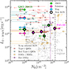 |
Fig. 1. Intrinsic 2 − 10 keV luminosity versus column density. Protocluster members are shown in cyan, magenta, and green. Diamonds indicate sources whose properties were derived via spectral fitting, while circles are for sources with properties derived from their hardness ratio (HR). Other classes of AGN detected in the X-ray are shown in different colors (Urrutia et al. 2005; Just et al. 2007; Wang et al. 2013; Banerji et al. 2014; Stern et al. 2014; Assef et al. 2016; Corral et al. 2016; Martocchia et al. 2017; Mountrichas et al. 2017; Ricci et al. 2017; Goulding et al. 2018; Vito et al. 2018a; Zappacosta et al. 2018; Li et al. 2019; Lansbury et al. 2020; Zou et al. 2020). Newly discovered AGN (i.e., not known as such prior to this work) are highlighted with thick black circles. |
For each protocluster, we performed a stacking analysis in the X-ray soft, hard, and full bands for sources that were not detected in the X-ray maps but were included in the prior catalogs (SMGs and LAEs). In addition, we also stacked SMGs and LAEs separately. No significant emission was found for any of the protoclusters as a result of this stacking analysis, which yielded effective exposure times in the full band of ∼9.5, 10, and 6 Ms.
For the optically selected QSOs in the three protoclusters, we also report in Table 3 the quantity  , where L2 keV and L2500 Å are the monochromatic luminosities at rest-frame 2 keV and 2500 Å, respectively (e.g., Brandt & Alexander 2015). This parameter is widely used to measure the relative emission of the hot corona and the accretion disk as a proxy for accretion physics (e.g., Lusso & Risaliti 2017). A well-known anti-correlation exists between αox and the UV luminosity of QSOs, implying that the contribution of the hot corona to the total QSO energy output decreases at high luminosities (e.g., Just et al. 2007). For the two QSOs in the Slug nebula, we obtained L2500 Å from the observed i-band magnitude in our LBT and LBC observations. For the two QSOs in the Fabulous protocluster, we measured the 1450 Å flux from the spectra presented by Arrigoni Battaia et al. (2018); for the optically selected QSO in the J0819 protocluster, we used the magnitude at 1450 Å reported in Arrigoni Battaia et al. (2018). In all cases, we assumed a typical QSO UV continuum Fν ∝ ν−α with α = 0.5 to derive the luminosity at rest-frame 2500 Å. The αox values found are in general agreement with the αox–LUV anti-correlations reported in the literature (e.g., Just et al. 2007; Lusso & Risaliti 2016). The slightly flatter αox value of compQSO in the Slug protocluster is consistent with its radio-loud nature (Cantalupo et al. 2014).
Properties of the X-ray-detected AGN in the three protoclusters derived using their HR.
4.2. X-ray diffuse emission
The gaseous halo surrounding quasar host galaxies is expected to be multiphase, with at least a cool (104 K) and a warm-hot (105 − 7 K) gas component (e.g., Costa et al. 2022; Obreja et al. 2024). While the cool gas is now routinely traced with Lyα observations, there is little to no information on the warm-hot gas phase at these redshifts. Acquiring information on this component is key to assessing the total baryon budget in the halo, and ultimately to constraining the strength of AGN feedback (e.g., Parimbelli et al. 2023). X-ray emission can, in principle, probe the hot gas component, but its levels are expected to be low (e.g., Bertone et al. 2010). Additionally, comparing the luminosity of the Lyα halo with that of the co-spatial X-ray emission can help disentangle the different origins of this radiation (Section 5.3). The potential diffuse X-ray emission is expected to peak in the soft part of the spectrum. Therefore, we investigated the presence of extended emission surrounding the central QSOs in the observed 1 − 2 keV band. The use of a narrow energy range reduces the contamination from the dominant QSO X-ray emission. Figure 2 shows the X-ray emission in the 1 − 2 keV range around the central QSOs of the Slug, Fabulous, and J0819. The QSOs correspond to the peak of the Lyα emission from the nebula. Upon visual inspection, QSO_Fabulous shows a possible excess of counts in the N-S direction (aligned with the nebula), and QSO_J0819 exhibits a circularly shaped excess of counts. In the case of UM287, we do not find any evidence for a potential extended emission.
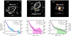 |
Fig. 2. X-ray maps in the 1 − 2 keV band of the central QSOs of the Slug, Fabulous, and J0819 protoclusters (upper panels) with Lyα contours in white. Background-subtracted differential radial profiles for the emission surrounding the Slug (cyan), Fabulous (magenta), and J0819 (green) central QSOs are shown in the bottom panels, with respect to the PSF prediction (purple line). The secondary y-axis is based on the apec model with a fixed temperature of 2 keV. |
To statistically investigate the nature of this emission, we performed simulations to reconstruct (via ray backtracing) the actual PSF of the observation at the position of the QSO, following a similar approach to Tozzi et al. (2022b) (but see also Fabbiano et al. 2017; Traina et al. 2021, for a similar approach). We obtained the PSF image with the following procedure. Using the CHART online tool (Carter et al. 2003), we simulated 10 different PSFs for each OBSID. Then, we used MARX and simulate_psf to produce an event file of each simulated image and subsequently merged each OBSID image to obtain the final merged simulated PSF image. Finally, we divided the emission by 10 to ensure that the number of counts was compatible with the actual emission. Once the simulated PSF images were produced, we compared the radial profiles obtained for the observed and simulated images. This comparison allowed us to determine whether the hint of extended emission around the QSO is statistically significant or if it can be ascribed to the PSF wings. Figure 2 shows this comparison for the three QSOs. In all cases, the X-ray radial profiles of the emission around the QSOs are consistent with the simulated PSF expectations within the errors. We thus conclude that our observations do not detect statistically significant extended X-ray emission at the positions of the ELANe.
5. Discussion
5.1. AGN fraction
Several recent studies have highlighted an enhancement of the fraction of AGN in protocluster environments with respect to the field (e.g., Tozzi et al. 2022a; Vito et al. 2024; Travascio et al. 2025). We compared the number of AGN in our sample with the number of sources in different parent samples of SMGs for all protoclusters and to LAEs in the Slug, where full LAE coverage is available across the field. Uncertainties on the fractions were calculated using binomial proportion intervals (Brown et al. 2001). The fraction of AGN among SMGs in the Slug is high (∼20%), as each of the three AGN is detected either with ALMA (continuum) or with SCUBA-2. The Fabulous and J0819 have similar AGN fractions (∼8 − 12%). For the Slug, we also computed the AGN fraction among LAEs. For the whole LAE sample, this fraction is low (∼0.04), but increases if we consider only the spectroscopically confirmed LAEs (corresponding to the brightest sub-sample of LAEs detected with the MMT,  ). These results are summarized in Table 5 and shown in Figure 3. The fractions we derive agree well with estimates from other works (see Vito et al. 2024, for a compilation). The Fabulous and J0819 have fractions of AGN among SMGs similar to those found for protoclusters at z ∼ 3 − 4.5, while the higher fraction found for the Slug protocluster is consistent with a slightly higher fraction expected at z ∼ 2 − 2.5, possibly linked to enhanced accretion activity at cosmic noon. This result is in agreement with the high AGN fraction in SMGs (i.e., fAGN ∼ 0.14) found in the Spiderweb protocluster at similar redshift. However, we note that the SMGs in the previous sample (i.e., Nowotka et al. 2022) are not spectroscopically confirmed, possibly leading to higher AGN fractions. At higher redshift, the SSA22 protocluster at z ∼ 3.2 has the largest known fraction of AGN to date (fAGN ∼ 0.5). The AGN fraction among LAEs is also similar to the lower fractions found in other protoclusters, consistent with LAEs being expected to reside in lower-mass halos than SMGs. These results show that the fraction of AGN in the ELAN candidate protocluster is consistent with that of other protoclusters and significantly higher than for low−z clusters.
Fractions of X-ray AGN to SMGs and LAEs.
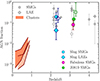 |
Fig. 3. Fractions of X-ray-selected AGN among different population of galaxies (i.e., SMGs and LAEs) in the Slug, Fabulous and J0819 protoclusters, compared to other protoclusters (Lehmer et al. 2009; Digby-North et al. 2010; Smail et al. 2014; Chen et al. 2016; Macuga et al. 2019; Umehata et al. 2019; Vito et al. 2020; Polletta et al. 2021; Tozzi et al. 2022a; Monson et al. 2023; Pérez-Martínez et al. 2023; Vito et al. 2024; Travascio et al. 2025) and the X-ray AGN fractions in local clusters (Martini et al. 2006; Bufanda et al. 2017). Empty blue and green points indicate the fractions computed for spectroscopically confirmed members (see Table 5). |
5.2. X-ray AGN luminosity function
As highlighted in Section 1, protoclusters have been found to foster SMBHs growth due to the large availability of gas. This enhancement affects both the normalization and shape of the X-ray luminosity function (XLF) (Tozzi et al. 2022a; Travascio et al. 2025; Vito et al. 2024). Previous studies have estimated the volume density (logΦ [Mpc−3 dex−1]) of AGN in protoclusters to be from 1 dex higher than in the field (z ∼ 2, Tozzi et al. 2022a), and up to 4 dex higher (z ∼ 4, Vito et al. 2024). Further investigations of the XLF at various redshifts are of key importance to understand how, and how quickly, black holes build up their masses in protoclusters at different cosmic epochs. In this section, we derive the volume density of the AGN in our sample, at z ∼ 2.2 (from the Slug protocluster) and at z ∼ 3.2 (from the Fabulous and J0819 AGN population) and compare these results with estimates obtained for other protoclusters at similar redshifts and with those in the field environment.
To estimate the procluster volumes, we considered two possible approaches. Firstly, we adopted, for each procluster, the same comoving volume used by Travascio et al. (2025) for MQN01 (which has among the best multiwavelength and spectroscopical coverage) to make a coherent comparison with their work. This “observed” volume is defined as V = 16 cMpc2 × 2000 km s−1. The comoving area (16 cMpc2) corresponds to the area of the MUSE field of view for MQN01 (∼2′×2′) and a size along the line of sight of ±1000 km s−1. For each protocluster, we converted the physical area into an angular size depending on the redshift of each system and considered only the sources falling within the 16 cMpc2 × 2000 km s−1 cube. This definition allows a coherent comparison with a previous studies focusing on the inner regions of protoclusters. Secondly, we used the predicted comoving radius at the relevant redshift in the simulation of Muldrew et al. (2015). The “observed” volumes correspond to 488, 441, and 440 cMpc3 for the Slug, Fabulous, and J0819, respectively. The second estimates were obtained from the Millennium Simulation (Springel et al. 2005) prediction of the average comoving radius enclosing 90% of the stellar mass in protocluster evolution with redshift. These are 13.2 (∼9500), 14.4 (∼12 500), and 14.4 (∼12 500) cMpc (cMpc3) for the Slug, J0819, and Fabulous protoclusters, respectively. We refer to this volume as the “predicted” volume. For the estimate of the AGN space densities of all protoclusters, we removed the central QSOs, since they were used to select the structures, and thus their inclusion would bias the XLF estimation.
We estimated the XLF in the two redshift bins by assuming the volumes defined above. This approach allows us to directly compare our results with the XLFs in blank fields reported in the literature (La Franca et al. 2005; Gilli et al. 2007; Ueda et al. 2014; Georgakakis et al. 2015; Vito et al. 2018b). The results are presented in Figure 4. We find that the XLF in protoclusters exceeds that observed in fields by a factor of 10 if we consider the protocluster radius predicted by simulations. When considering the “observed” volume this difference increases up to two orders of magnitude.
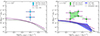 |
Fig. 4. X-ray luminosity functions in two different redshift bins (z ∼ 2.2 and z ∼ 3.2) and in luminosity bins of 0.5 dex. Our data are shown as cyan and green points, with different markers representing different assumptions on the co-moving volume. For comparison, XLFs for the field environment at similar redshifts are also reported. The solid purple line shows the XLF for field AGN from Gilli et al. (2007). The dashed lines correspond to the XLFs from Ueda et al. (2014) at z ∼ 2.2 and z ∼ 3.2. The dotted line shows the XLF from Georgakakis et al. (2015), and the purple shaded area represents the XLF estimated by Vito et al. (2018b). |
Following the approach of Travascio et al. (2025), we also estimated the cumulative space density in the three protoclusters. Specifically, we calculated the cumulative AGN distribution and divided it by the comoving volume. To consistently compare our results with Travascio et al. (2025), we assumed the same volume as defined earlier. The results are shown in Figure 5, where the cumulative AGN space densities are plotted with errors derived using Gerhels estimates for low statistics (Nobj < 10). Due to the similar redshift, we combined the Fabulous and J0819 results into a single estimate by summing both the number of AGN and the volumes of the two structures. In the lower redshift bin, where the cumulative space density is obtained from the Slug sources, the cumulative space density is slightly lower than that found in the Spiderweb protocluster at similar redshift (Tozzi et al. 2022a; Travascio et al. 2025), although consistent within uncertainties. It also shows an excess of approximately 3 dex compared to fields. Similarly, in the second redshift bin, the cumulative space densities differ significantly from those found in field environments (Gilli et al. 2007), with a ∼2 − 3 dex discrepancy found using the same volume as Travascio et al. (2025). Although most members of these structures remain spectroscopically unconfirmed, we find an overall agreement with the results of Travascio et al. (2025) for the MQN01 and SSA22 protoclusters. However, it should be noted that our observations are shallower than those by Tozzi et al. (2022a) (700 ks) and Travascio et al. (2025) (630 ks), resulting in a shallower lower limit in the probed luminosities of the detected sources.
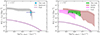 |
Fig. 5. Cumulative space density in two redshift bins (z ∼ 2.2 and z ∼ 3.2). Our data are shown as a cyan point and a green shaded area, where the uncertainties are computed according to Gehrels (1986). For comparison, the cumulative space densities of other protoclusters at similar redshifts are also reported. The gray shaded region (left panel) represents the cumulative space density for the Spiderweb protocluster (see Tozzi et al. 2022a; Travascio et al. 2025), while the red and pink shaded areas (right panel) correspond to the MQN01 and SSA22 by Travascio et al. (2025). The purple solid line shows the cumulative space density for field AGN from Gilli et al. (2007). |
To assess whether the larger number of AGN observed in protoclusters reflects the higher density of galaxies or is instead the product of faster SMBH growth, we compared the ratio between the number density of AGN in the protoclusters to that in the field (i.e., AGN overdensity) with the same ratio computed for galaxies (i.e., galaxy overdensity). This analysis was conducted using the “observed” volumes of the protoclusters. A similar protocluster-to-field ratio for AGN and galaxies would indicate that the higher AGN numbers in protoclusters result directly from the galaxy overdensity. If instead the AGN ratio is higher than the galaxy ratio, we can conclude that the SMBH growth is directly enhanced in overdense regions of the Universe. To compute these ratios, we assumed an XLF for AGN and IR-LF for SMGs in fields. In particular, we assumed the Gilli et al. (2007) XLF3 for AGN and the IR-LF by Traina et al. (2024) for SMGs. By integrating these curves, we obtain the number density of each galaxy population. Multiplying by the protocluster volume then yields the expected number of field galaxies within that volume. The LFs were integrated down to the luminosity of the faintest member of the corresponding population in our targets (thus taking into account the sensitivity of the observations). For the SMGs, we converted observed sub-mm fluxes into infrared 8 − 1000 μm luminosities by assuming that the SEDs of our SMGs are similar to the median SED from the Automated mining of the ALMA Archive in COSMOS (A3COSMOS4; Liu et al. 2019; Adscheid et al. 2024; Traina et al. 2024). We then compared the expected number of sources with those observed in the protoclusters, estimating the AGN and SMGs protocluster-to-field ratios. The results of this comparison as a function of redshift are shown in Figure 6 (left panel). For the Slug protocluster, the AGN overdensity is higher (by a factor ≳100) than that of SMGs. The discrepancy is smaller for the Fabulous and J0819 protoclusters, where the difference is a factor ∼10. For comparison, we computed the same ratios for other protoclusters from the literature, allowing us to cover a broader redshift range. In particular, we considered the Spiderweb (z ∼ 2.16), MQN01 (z ∼ 3.2), DRC (z ∼ 4), and SPT2349-56 (z ∼ 4.3) protoclusters. The ratios were computed in the same manner as for our sample. We also find a significant discrepancy between the AGN and SMGs enhancements in these protoclusters, suggesting the ubiquity of this phenomenon at all redshifts. In addition, these results suggest an increasing trend with redshift for the enhanced SMBH activity in protoclusters (noting that for SPT we derived a lower limit due to the lower limit on the X-ray luminosity of the faintest member). However, the SMG overdensity also increases with redshift. To investigate whether a redshift evolution is present in the AGN-to-SMGs enhancement, we derived the ratios of the two overdensities for all the protoclusters (see Figure 6, right panel). We find that all these structures exhibit AGN enhancements significantly higher than those of SMGs. In addition, this enhancement does not appear to change with the overdensity of SMGs (i.e., the larger density of AGN does not depend on the size of the overdensity). In conclusion, our volume density estimates, together with additional observational evidence from other studies at similar or higher redshifts (see e.g., Tozzi et al. 2022a; Travascio et al. 2025; Vito et al. 2024) support a scenario in which SMBH growth, and thus the phenomena of active nuclei, is significantly favored in overdense regions of the Universe, where more gas is available to fuel and infall into the nuclear region of galaxies. Moreover, the discrepancy with field is enhanced at higher X-ray luminosities, where protocluster XLFs show a roughly flat trend (Figures 4 and 5), without a significant decrease in volume density. This further supports the scenario of the faster formation of SMBH of larger masses.
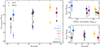 |
Fig. 6. Left panel: Ratio of the number density of objects in the three protoclusters to that in the field, for AGN (stars) and SMGs (circles). Errors are computed in the Poissonian assumption. The environment of AGN with respect to field in our targets is 1–2 dex larger than overdensity of the parent population of galaxies, impliying a direct environmental effect on the SMBH growth in these structures. We also show the ratios for other protoclusters at various redshifts (Tozzi et al. 2022a; Vito et al. 2020, 2024; Travascio et al. 2025). Right panel: Ratio of AGN to SMG overdensity, as a function of SMG overdensity (top) and redshift (bottom), for the same protoclusters. |
5.3. Contribution of cooling radiation on ELAN emission
Since we do not detect any significant extended X-ray (1-2 keV) emission co-spatial with the ELAN in the Slug, J0819, and Fabulous protoclusters, we derive a 3σ upper limit on the observed flux and intrinsic X-ray luminosity for the diffuse emission in this section. If some of the Lyα emission is not powered by the bright QSOs– for example, as a result of photoionization or Lyα photon-pumping (see e.g., Cantalupo 2017, for a review)– then, despite the fact that the ionizing power of the AGN in the protoclusters is more than one dex higher than that required to power the nebula (Umehata et al. 2019), these estimates can still provide constraints on additional or alternative powering mechanisms. One such possibility is the so-called Lyα cooling (see e.g., Rosdahl & Blaizot 2012), which has been proposed to explain extended Lyα emission without clear photoionization sources, or Lyα blobs (LAB; see e.g., Geach et al. 2009; Daddi et al. 2021). In particular, if a significant fraction of the gas is not photoionized by the quasar (e.g., because the quasar is young or the opening angle of the emission is very small), we can estimate the expected LX/LLyα ratio produced by a cooling flow in collisional ionization equilibrium. Following the works of Bower et al. (2004) and Geach et al. (2009), the conservation of angular momentum in subsonic cooling flows implies LX/LLyα > 1000 if the Lyα emission is produced by Lyα collisional excitation of energetic electrons powered by gravitational heating (so-called “Lyα cooling”). Conversely, if LX/LLyα < 1, this indicates that, under these assumptions, the majority of the nebular emission is unrelated to Lyα cooling. We derived the 3σ upper limits on the ELAN X-ray fluxes and luminosities in regions surrounding the central QSOs. We extracted the X-ray spectra and ancillary files from an annular region (inner radius = 2″, outer radius = 4″) centered on the QSO. Since the emission is not point-like, we ran specextract with the weight=True option, which enables for the weighting of the ARF and RMF associated with the extracted spectra. We then obtained the 3σ upper limits on the 1 − 2 keV fluxes and corresponding rest-frame ∼4 − 8 keV intrinsic luminosities, to enable direct comparison with the results of Geach et al. (2009). This was done by scaling the upper limits on the net counts in these regions, assuming an intrinsic spectrum modeled with Γ ∼ 1.8. We constrain the X-ray luminosities of the ELANe to be < 7.2 × 1043 erg s−1, < 8 × 1043 erg s−1, and < 1.1 × 1043 erg s−1 for the Fabulous, J0819, and Slug, respectively. Considering their Lyα luminosities of LLyα ∼ 3.2 × 1044 erg s−1, LLyα ∼ 4 × 1044 erg s−1, and LLyα ∼ 2 × 1044 erg s−1, we estimate LX/LLyα < 0.2, 0.2 ,and 0.06, respectively. Figure 7 compares our results with those from the literature. Three different regions are highlighted: the gray region, with LX < LLyα, contains sources for which a cooling explanation of the ELAN emission is unlikely; the purple region, where LX > 1000 × LLyα, in which the ELAN emission is consistent with gravitational cooling processes; and the white region which includes sources with intermediate values of LX/LLyα. Out of 29 extended Lyα emission regions in the SSA22 protocluster, only five have been detected in X-rays, while for the remaining 24, upper limits were derived by Geach et al. (2009). Specifically, these five X-ray-detected extended Lyα emissions belong to the intermediate region, meaning no strong constraint can be placed on the origin of their emission. The stacked X-ray emission from the SSA22 extended Lyα emission lies in the gray region of the plot, thus their main powering mechanism cannot be gravitational cooling. Other extended Lyα emissions, in the Boötes and GOODS-S fields are either in the intermediate region or undetected in X-rays (Nilsson et al. 2006; Yang et al. 2009). Similarly, four high redshift radio galaxies (HzRGs) studied by Reuland et al. (2003) are detected in the X-rays, but remain within the gray or white areas. We present the comparison of Lyα-Xray luminosities for the Spiderweb protocluster (Tozzi et al. 2022b), where an extended diffuse emission is clearly detected in the X-rays. In this case, we consider the total (i.e., including contaminant sources such as the jets) for both the X-ray and Lyα luminosity, as a value of LLyα is not available. Its X-ray luminosity is almost 5 × 1045 erg s−1, compatible with the luminosity of the total Lyα emission, placing the Spiderweb in the middle region where cooling cannot be ruled-out. Like most of the undetected sources, the three ELANe in our analysis lie within the gray region, where, as expected, gravitational cooling is not the mechanism responsible for the nebula emission.
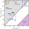 |
Fig. 7. X-ray vs Lyα luminosity of the extended emission from the ELANe. Magenta, green, and cyan circles represent the Fabulous, J0819, and Slug nebulae, respectively. Blue and white points show SSA22 extended Lyα emission reported by Geach et al. (2009); orange circles represent extended Lyα emission around HzRGs from Reuland et al. (2003); pink circles and squares correspond to extended Lyα emission in the Boötes and GOODS-S fields, respectively (Yang et al. 2009; Nilsson et al. 2006); the red circle marks the Spiderweb extended Lyα nebula fromTozzi et al. (2022b), and the white circle marks the LAB from Daddi et al. (2021). The solid black line represents the 1:1 relation (Geach et al. 2009), while the dashed black line indicates the LX = 1000LLyα relation (Cowie et al. 1980; Bower et al. 2004). The purple region (lower left) corresponds to the scenario in which the main powering channel of the extended Lyα emission is gravitational cooling. The gray area (upper right), represents the region in which the cooling cannot be the fueling mechanism of the nebula. |
6. Conclusions
In this paper we present deep Chandra observations (∼190 ks, ∼240 ks, and ∼280 ks) of three protoclusters (Slug, Fabulous, and J0819) at z ∼ 2 and z ∼ 3. The three protoclusters show evidence of large gas reservoirs in their inner regions, with enormous Lyα nebulae extending for several kiloparsecs. Here, we summarize the results from our dedicated X-ray analysis of point-like sources as well as the lack of diffuse emission surrounding the central QSOs. We also discuss the implications of these results on the fast growth of SMBHs in overdense regions of the Universe.
-
We detected a total of 11 X-ray AGN in the three protoclusters, six of which are reported here as AGN for the first time. Most of the detected AGN (none out of 11) are hosted in SMGs, while only five (which are the QSOs) are also LAEs.
-
The main properties of the nuclear emission in these sources were obtained either via spectral analysis (for AGN with more than 30 net counts) or via their hardness ratios. The bright QSOs at the centers of the ELANe show similar photon indices and are unabsorbed. Their 2 − 10 X-ray luminosities exceed 1045 erg s−1, placing them among the brightest X-ray sources. In particular, QSO_J0819 is the most luminous source in our sample, with LX ∼ 6 × 1045 erg s−1. The other AGN do not exhibit peculiar properties, except for one Fabulous AGN (Fab-33) which is identified as a Compton-thick candidate.
-
We investigated the presence of potential diffuse emission co-spatial with the ELANe by comparing the observed radial profiles around the central QSOs with the simulated PSFs of each image. The emission around the QSOs is consistent with the shape of the Chandra PSF, ruling out a significant contribution from extended emission in our data. Nevertheless, we measured an upper limit on the X-ray luminosity around the QSOs, which allowed us to rule out a cooling scenario for the supply of the Lyα nebulae.
-
In good agreement with recent studies of the XLF in protoclusters, we find that the XLF of the Slug (at z ∼ 2.2) and of the Fabulous and J0819 protoclusters (at z ∼ 3.2) is ∼1 − 2 orders of magnitude higher than that of AGN in the field. This confirms the larger number of AGN in these overdense environments, where we measure AGN fractions of 10 − 20%.
-
This higher density of AGN cannot be solely attributed to the higher number of galaxies in the protocluster. Indeed, we find that the ratio of protocluster-to-field AGN is significantly higher than the corresponding ratio for SMGs using homogeneous flux limits. This supports a scenario in which overdense, gas-rich environments directly enhance the growth of SMBHs in the member galaxies.
In the coming years, several current and future facilities (e.g., Roman, Euclid, SKA) will be of fundamental importance in the detection and characterization of protoclusters at high redshift. Their contributions, combined with the potential of the AXIS probe, will significantly improve our understanding of the AGN content of such structures. This will ultimately allow us to understand how these environments favor the formation of the most massive SMBHs in the Universe.
The MyTORUS code is a physically motivated model, widely used in the X-ray spectral analysis of Compton-thick sources, based on three tables for the zeroth-order emission component, the scattered continuum, and the iron line emission component.
Acknowledgments
AT, FV, CV, PT, RG acknowledge support from the “INAF Ricerca Fondamentale 2023 – Large GO” grant. C.-C.C. acknowledges support from the National Science and Technology Council of Taiwan (111-2112-M-001-045-MY3), as well as Academia Sinica through the Career Development Award (AS-CDA-112-M02). AP acknowledges support from Fondazione Cariplo grant no. 2020-0902. SC gratefully acknowledges support from the European Research Council (ERC) under the European Union’s Horizon 2020 Research and Innovation programme grant agreement No 864361.
References
- Adscheid, S., Magnelli, B., Liu, D., et al. 2024, A&A, 685, A1 [NASA ADS] [CrossRef] [EDP Sciences] [Google Scholar]
- Aird, J., Coil, A. L., Moustakas, J., et al. 2012, ApJ, 746, 90 [CrossRef] [Google Scholar]
- Aird, J., Coil, A. L., Georgakakis, A., et al. 2015, MNRAS, 451, 1892 [Google Scholar]
- Aird, J., Coil, A. L., & Georgakakis, A. 2018, MNRAS, 474, 1225 [NASA ADS] [CrossRef] [Google Scholar]
- Alberts, S., & Noble, A. 2022, Universe, 8, 554 [Google Scholar]
- Arrigoni Battaia, F., Chen, C.-C., Fumagalli, M., et al. 2018, A&A, 620, A202 [NASA ADS] [CrossRef] [EDP Sciences] [Google Scholar]
- Arrigoni Battaia, F., Hennawi, J. F., Prochaska, J. X., et al. 2019, MNRAS, 482, 3162 [NASA ADS] [CrossRef] [Google Scholar]
- Arrigoni Battaia, F., Chen, C.-C., Liu, H.-Y. B., et al. 2022, ApJ, 930, 72 [NASA ADS] [CrossRef] [Google Scholar]
- Arrigoni Battaia, F., Obreja, A., Chen, C. C., et al. 2023, A&A, 676, A51 [NASA ADS] [CrossRef] [EDP Sciences] [Google Scholar]
- Assef, R. J., Eisenhardt, P. R. M., Stern, D., et al. 2015, ApJ, 804, 27 [Google Scholar]
- Assef, R. J., Walton, D. J., Brightman, M., et al. 2016, ApJ, 819, 111 [Google Scholar]
- Bacon, R., Accardo, M., Adjali, L., et al. 2010, SPIE Conf. Ser., 7735, 773508 [Google Scholar]
- Bădescu, T., Yang, Y., Bertoldi, F., et al. 2017, ApJ, 845, 172 [Google Scholar]
- Banerji, M., Fabian, A. C., & McMahon, R. G. 2014, MNRAS, 439, L51 [CrossRef] [Google Scholar]
- Bertin, E., & Arnouts, S. 1996, A&AS, 117, 393 [NASA ADS] [CrossRef] [EDP Sciences] [Google Scholar]
- Bertone, S., Schaye, J., Dalla Vecchia, C., et al. 2010, MNRAS, 407, 544 [NASA ADS] [CrossRef] [Google Scholar]
- Bongiorno, A., Merloni, A., Brusa, M., et al. 2012, MNRAS, 427, 3103 [Google Scholar]
- Bongiorno, A., Schulze, A., Merloni, A., et al. 2016, A&A, 588, A78 [NASA ADS] [CrossRef] [EDP Sciences] [Google Scholar]
- Boquien, M., Burgarella, D., Roehlly, Y., et al. 2019, A&A, 622, A103 [NASA ADS] [CrossRef] [EDP Sciences] [Google Scholar]
- Borisova, E., Cantalupo, S., Lilly, S. J., et al. 2016, ApJ, 831, 39 [Google Scholar]
- Bower, R. G., Morris, S. L., Bacon, R., et al. 2004, MNRAS, 351, 63 [Google Scholar]
- Brandt, W. N., & Alexander, D. M. 2015, A&ARv, 23, 1 [Google Scholar]
- Brown, L. D., Cai, T. T., & DasGupta, A. 2001, Stat. Sci., 16, 101 [Google Scholar]
- Bruzual, G., & Charlot, S. 2003, MNRAS, 344, 1000 [NASA ADS] [CrossRef] [Google Scholar]
- Bufanda, E., Hollowood, D., Jeltema, T. E., et al. 2017, MNRAS, 465, 2531 [NASA ADS] [CrossRef] [Google Scholar]
- Cai, Z., Fan, X., Yang, Y., et al. 2017, ApJ, 837, 71 [NASA ADS] [CrossRef] [Google Scholar]
- Cantalupo, S. 2017, Astrophys. Space Sci. Libr., 430, 195 [Google Scholar]
- Cantalupo, S., Arrigoni-Battaia, F., Prochaska, J. X., Hennawi, J. F., & Madau, P. 2014, Nature, 506, 63 [Google Scholar]
- Carraro, R., Rodighiero, G., Cassata, P., et al. 2020, A&A, 642, A65 [EDP Sciences] [Google Scholar]
- Carter, C., Karovska, M., Jerius, D., Glotfelty, K., & Beikman, S. 2003, ASP Conf. Ser., 295, 477 [NASA ADS] [Google Scholar]
- Chabrier, G. 2003, PASP, 115, 763 [Google Scholar]
- Charlot, S., & Fall, S. M. 2000, ApJ, 539, 718 [Google Scholar]
- Chen, C.-C., Smail, I., Swinbank, A. M., et al. 2016, ApJ, 831, 91 [NASA ADS] [CrossRef] [Google Scholar]
- Chen, C.-C., Arrigoni Battaia, F., Emonts, B. H. C., Lehnert, M. D., & Prochaska, J. X. 2021, ApJ, 923, 200 [NASA ADS] [CrossRef] [Google Scholar]
- Chiang, Y.-K., Overzier, R., & Gebhardt, K. 2014, ApJ, 782, L3 [NASA ADS] [CrossRef] [Google Scholar]
- Chiang, Y.-K., Overzier, R. A., Gebhardt, K., et al. 2015, ApJ, 808, 37 [NASA ADS] [CrossRef] [Google Scholar]
- Chiang, Y.-K., Overzier, R. A., Gebhardt, K., & Henriques, B. 2017, ApJ, 844, L23 [Google Scholar]
- Ciardullo, R., Gronwall, C., Adams, J. J., et al. 2013, ApJ, 769, 83 [Google Scholar]
- Corral, A., Georgantopoulos, I., Comastri, A., et al. 2016, A&A, 592, A109 [NASA ADS] [CrossRef] [EDP Sciences] [Google Scholar]
- Costa, T., Arrigoni Battaia, F., Farina, E. P., et al. 2022, MNRAS, 517, 1767 [NASA ADS] [CrossRef] [Google Scholar]
- Cowie, L. L., Fabian, A. C., & Nulsen, P. E. J. 1980, MNRAS, 191, 399 [Google Scholar]
- Cucciati, O., Zamorani, G., Lemaux, B. C., et al. 2014, A&A, 570, A16 [NASA ADS] [CrossRef] [EDP Sciences] [Google Scholar]
- Daddi, E., Valentino, F., Rich, R. M., et al. 2021, A&A, 649, A78 [NASA ADS] [CrossRef] [EDP Sciences] [Google Scholar]
- Dannerbauer, H., Kurk, J. D., De Breuck, C., et al. 2014, A&A, 570, A55 [NASA ADS] [CrossRef] [EDP Sciences] [Google Scholar]
- De Breuck, C., Bertoldi, F., Carilli, C., et al. 2004, A&A, 424, 1 [NASA ADS] [CrossRef] [EDP Sciences] [Google Scholar]
- Digby-North, J. A., Nandra, K., Laird, E. S., et al. 2010, MNRAS, 407, 846 [NASA ADS] [CrossRef] [Google Scholar]
- Draine, B. T., Aniano, G., Krause, O., et al. 2014, ApJ, 780, 172 [Google Scholar]
- Duras, F., Bongiorno, A., Ricci, F., et al. 2020, A&A, 636, A73 [NASA ADS] [CrossRef] [EDP Sciences] [Google Scholar]
- Elford, J. S., Davis, T. A., Ruffa, I., et al. 2024, MNRAS, 528, 319 [NASA ADS] [CrossRef] [Google Scholar]
- Fabbiano, G., Elvis, M., Paggi, A., et al. 2017, ApJ, 842, L4 [NASA ADS] [CrossRef] [Google Scholar]
- Ferrarese, L. 2002, ApJ, 578, 90 [NASA ADS] [CrossRef] [Google Scholar]
- Fruscione, A., McDowell, J. C., Allen, G. E., et al. 2006, SPIE Conf. Ser., 6270, 62701V [Google Scholar]
- Gaia Collaboration (Vallenari, A., et al.) 2023, A&A, 674, A1 [NASA ADS] [CrossRef] [EDP Sciences] [Google Scholar]
- Galbiati, M., Cantalupo, S., Steidel, C., et al. 2025, A&A, 696, A95 [NASA ADS] [CrossRef] [EDP Sciences] [Google Scholar]
- Geach, J. E., Alexander, D. M., Lehmer, B. D., et al. 2009, ApJ, 700, 1 [Google Scholar]
- Gehrels, N. 1986, ApJ, 303, 336 [Google Scholar]
- Georgakakis, A., Aird, J., Buchner, J., et al. 2015, MNRAS, 453, 1946 [Google Scholar]
- Gilli, R., Comastri, A., & Hasinger, G. 2007, A&A, 463, 79 [NASA ADS] [CrossRef] [EDP Sciences] [Google Scholar]
- Gilli, R., Mignoli, M., Peca, A., et al. 2019, A&A, 632, A26 [NASA ADS] [CrossRef] [EDP Sciences] [Google Scholar]
- Gordon, C., & Arnaud, K. 2021, Astrophysics Source Code Library [record ascl:2101.014] [Google Scholar]
- Goulding, A. D., Zakamska, N. L., Alexandroff, R. M., et al. 2018, ApJ, 856, 4 [Google Scholar]
- Haiman, Z., Kocsis, B., & Menou, K. 2009, ApJ, 700, 1952 [CrossRef] [Google Scholar]
- Hatch, N. A., Wylezalek, D., Kurk, J. D., et al. 2014, MNRAS, 445, 280 [NASA ADS] [CrossRef] [Google Scholar]
- Hennawi, J. F., Prochaska, J. X., Cantalupo, S., & Arrigoni-Battaia, F. 2015, Science, 348, 779 [Google Scholar]
- Just, D. W., Brandt, W. N., Shemmer, O., et al. 2007, ApJ, 665, 1004 [Google Scholar]
- Kashino, D., Lilly, S. J., Matthee, J., et al. 2023, ApJ, 950, 66 [CrossRef] [Google Scholar]
- Kormendy, J., & Ho, L. C. 2013, ARA&A, 51, 511 [Google Scholar]
- La Franca, F., Fiore, F., Comastri, A., et al. 2005, ApJ, 635, 864 [NASA ADS] [CrossRef] [Google Scholar]
- Lansbury, G. B., Banerji, M., Fabian, A. C., & Temple, M. J. 2020, MNRAS, 495, 2652 [Google Scholar]
- Lehmer, B. D., Alexander, D. M., Chapman, S. C., et al. 2009, MNRAS, 400, 299 [Google Scholar]
- Lehmer, B. D., Lucy, A. B., Alexander, D. M., et al. 2013, ApJ, 765, 87 [NASA ADS] [CrossRef] [Google Scholar]
- Li, J., Xue, Y., Sun, M., et al. 2019, ApJ, 877, 5 [NASA ADS] [CrossRef] [Google Scholar]
- Liu, D., Schinnerer, E., Groves, B., et al. 2019, ApJ, 887, 235 [Google Scholar]
- Liu, S., Zheng, X. Z., Shi, D. D., et al. 2023, MNRAS, 523, 2422 [CrossRef] [Google Scholar]
- Lusso, E., & Risaliti, G. 2016, ApJ, 819, 154 [Google Scholar]
- Lusso, E., & Risaliti, G. 2017, A&A, 602, A79 [NASA ADS] [CrossRef] [EDP Sciences] [Google Scholar]
- Macuga, M., Martini, P., Miller, E. D., et al. 2019, ApJ, 874, 54 [NASA ADS] [CrossRef] [Google Scholar]
- Magorrian, J., Tremaine, S., Richstone, D., et al. 1998, AJ, 115, 2285 [Google Scholar]
- Marchesi, S., Mignoli, M., Gilli, R., et al. 2023, A&A, 673, A97 [NASA ADS] [CrossRef] [EDP Sciences] [Google Scholar]
- Martini, P., Kelson, D. D., Kim, E., Mulchaey, J. S., & Athey, A. A. 2006, ApJ, 644, 116 [NASA ADS] [CrossRef] [Google Scholar]
- Martini, P., Miller, E. D., Brodwin, M., et al. 2013, ApJ, 768, 1 [Google Scholar]
- Martocchia, S., Piconcelli, E., Zappacosta, L., et al. 2017, A&A, 608, A51 [NASA ADS] [CrossRef] [EDP Sciences] [Google Scholar]
- Monson, E. B., Doore, K., Eufrasio, R. T., et al. 2023, ApJ, 951, 15 [NASA ADS] [CrossRef] [Google Scholar]
- Mori, M., Umemura, M., & Ferrara, A. 2004, ApJ, 613, L97 [NASA ADS] [CrossRef] [Google Scholar]
- Mountrichas, G., Georgantopoulos, I., Secrest, N. J., et al. 2017, MNRAS, 468, 3042 [NASA ADS] [CrossRef] [Google Scholar]
- Muldrew, S. I., Hatch, N. A., & Cooke, E. A. 2015, MNRAS, 452, 2528 [NASA ADS] [CrossRef] [Google Scholar]
- Murphy, K. D., & Yaqoob, T. 2009, MNRAS, 397, 1549 [Google Scholar]
- Nilsson, K. K., Fynbo, J. P. U., Møller, P., Sommer-Larsen, J., & Ledoux, C. 2006, A&A, 452, L23 [NASA ADS] [CrossRef] [EDP Sciences] [Google Scholar]
- Nowotka, M., Chen, C. C., Battaia, F. A., et al. 2022, VizieR On-line Data Catalog: J/A+A/658/A77 [Google Scholar]
- Obreja, A., Arrigoni Battaia, F., Macciò, A. V., & Buck, T. 2024, MNRAS, 527, 8078 [Google Scholar]
- Oteo, I., Ivison, R. J., Dunne, L., et al. 2018, ApJ, 856, 72 [Google Scholar]
- Ouchi, M., Shimasaku, K., Akiyama, M., et al. 2005, ApJ, 620, L1 [NASA ADS] [CrossRef] [Google Scholar]
- Overzier, R. A. 2016, A&ARv, 24, 14 [Google Scholar]
- Overzier, R. A., Bouwens, R. J., Cross, N. J. G., et al. 2008, ApJ, 673, 143 [NASA ADS] [CrossRef] [Google Scholar]
- Overzier, R. A., Nesvadba, N. P. H., Dijkstra, M., et al. 2013, ApJ, 771, 89 [NASA ADS] [CrossRef] [Google Scholar]
- Padovani, P., Alexander, D. M., Assef, R. J., et al. 2017, A&ARv, 25, 2 [Google Scholar]
- Parimbelli, G., Branchini, E., Viel, M., Villaescusa-Navarro, F., & ZuHone, J. 2023, MNRAS, 523, 2263 [NASA ADS] [CrossRef] [Google Scholar]
- Pensabene, A., Cantalupo, S., Cicone, C., et al. 2024, A&A, 684, A119 [NASA ADS] [CrossRef] [EDP Sciences] [Google Scholar]
- Pentericci, L., Kurk, J. D., Röttgering, H. J. A., et al. 2000, A&A, 361, L25 [NASA ADS] [Google Scholar]
- Pérez-Martínez, J. M., Dannerbauer, H., Kodama, T., et al. 2023, MNRAS, 518, 1707 [Google Scholar]
- Planck Collaboration VI. 2020, A&A , 641, A6 [NASA ADS] [CrossRef] [EDP Sciences] [Google Scholar]
- Polletta, M., Soucail, G., Dole, H., et al. 2021, A&A, 654, A121 [NASA ADS] [CrossRef] [EDP Sciences] [Google Scholar]
- Prescott, M. K. M., Kashikawa, N., Dey, A., & Matsuda, Y. 2008, ApJ, 678, L77 [NASA ADS] [CrossRef] [Google Scholar]
- Prochaska, J. X., Madau, P., O’Meara, J. M., & Fumagalli, M. 2014, MNRAS, 438, 476 [NASA ADS] [CrossRef] [Google Scholar]
- Reuland, M., van Breugel, W., Röttgering, H., et al. 2003, ApJ, 592, 755 [CrossRef] [Google Scholar]
- Ricci, C., Assef, R. J., Stern, D., et al. 2017, ApJ, 835, 105 [Google Scholar]
- Rosdahl, J., & Blaizot, J. 2012, MNRAS, 423, 344 [Google Scholar]
- Smail, I., Geach, J. E., Swinbank, A. M., et al. 2014, ApJ, 782, 19 [NASA ADS] [CrossRef] [Google Scholar]
- Speagle, J. S., Steinhardt, C. L., Capak, P. L., & Silverman, J. D. 2014, ApJS, 214, 15 [Google Scholar]
- Springel, V., White, S. D. M., Jenkins, A., et al. 2005, Nature, 435, 629 [Google Scholar]
- Stalevski, M., Fritz, J., Baes, M., Nakos, T., & Popović, L. Č. 2012, MNRAS, 420, 2756 [Google Scholar]
- Stalevski, M., Ricci, C., Ueda, Y., et al. 2016, MNRAS, 458, 2288 [Google Scholar]
- Steidel, C. C., Adelberger, K. L., Shapley, A. E., et al. 2000, ApJ, 532, 170 [NASA ADS] [CrossRef] [Google Scholar]
- Steidel, C. C., Adelberger, K. L., Shapley, A. E., et al. 2005, ApJ, 626, 44 [NASA ADS] [CrossRef] [Google Scholar]
- Stern, D., Lansbury, G. B., Assef, R. J., et al. 2014, ApJ, 794, 102 [Google Scholar]
- Stroe, A., Sobral, D., Matthee, J., Calhau, J., & Oteo, I. 2017, MNRAS, 471, 2575 [NASA ADS] [CrossRef] [Google Scholar]
- Toshikawa, J., Kashikawa, N., Overzier, R., et al. 2016, ApJ, 826, 114 [NASA ADS] [CrossRef] [Google Scholar]
- Tozzi, P., Pentericci, L., Gilli, R., et al. 2022a, A&A, 662, A54 [NASA ADS] [CrossRef] [EDP Sciences] [Google Scholar]
- Tozzi, P., Gilli, R., Liu, A., et al. 2022b, A&A, 667, A134 [NASA ADS] [CrossRef] [EDP Sciences] [Google Scholar]
- Traina, A., Marchesi, S., Vignali, C., et al. 2021, ApJ, 922, 159 [NASA ADS] [CrossRef] [Google Scholar]
- Traina, A., Gruppioni, C., Delvecchio, I., et al. 2024, A&A, 681, A118 [NASA ADS] [CrossRef] [EDP Sciences] [Google Scholar]
- Travascio, A., Cantalupo, S., Tozzi, P., et al. 2025, A&A, 694, A165 [NASA ADS] [CrossRef] [EDP Sciences] [Google Scholar]
- Ueda, Y., Akiyama, M., Hasinger, G., Miyaji, T., & Watson, M. G. 2014, ApJ, 786, 104 [Google Scholar]
- Umehata, H., Tamura, Y., Kohno, K., et al. 2017, ApJ, 835, 98 [Google Scholar]
- Umehata, H., Fumagalli, M., Smail, I., et al. 2019, Science, 366, 97 [Google Scholar]
- Urrutia, T., Lacy, M., Gregg, M. D., & Becker, R. H. 2005, ApJ, 627, 75 [Google Scholar]
- Venemans, B. P., Röttgering, H. J. A., Miley, G. K., et al. 2007, A&A, 461, 823 [NASA ADS] [CrossRef] [EDP Sciences] [Google Scholar]
- Vito, F., Brandt, W. N., Stern, D., et al. 2018a, MNRAS, 474, 4528 [Google Scholar]
- Vito, F., Brandt, W. N., Yang, G., et al. 2018b, MNRAS, 473, 2378 [Google Scholar]
- Vito, F., Brandt, W. N., Lehmer, B. D., et al. 2020, A&A, 642, A149 [NASA ADS] [CrossRef] [EDP Sciences] [Google Scholar]
- Vito, F., Brandt, W. N., Comastri, A., et al. 2024, A&A, 689, A130 [NASA ADS] [CrossRef] [EDP Sciences] [Google Scholar]
- Wang, S. X., Brandt, W. N., Luo, B., et al. 2013, ApJ, 778, 179 [NASA ADS] [CrossRef] [Google Scholar]
- Yang, Y., Zabludoff, A., Tremonti, C., Eisenstein, D., & Davé, R. 2009, ApJ, 693, 1579 [NASA ADS] [CrossRef] [Google Scholar]
- Zappacosta, L., Piconcelli, E., Duras, F., et al. 2018, A&A, 618, A28 [NASA ADS] [CrossRef] [EDP Sciences] [Google Scholar]
- Zou, F., Brandt, W. N., Vito, F., et al. 2020, MNRAS, 499, 1823 [NASA ADS] [CrossRef] [Google Scholar]
- Zou, F., Brandt, W. N., Chen, C.-T., et al. 2022, ApJS, 262, 15 [NASA ADS] [CrossRef] [Google Scholar]
Appendix A: X-ray detections
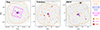 |
Fig. A.1. Chandra X-ray maps (gray scale) of the three fields, centered on the aim point. The coverage of ancillary data is superimposed as colored contours (orange, blue, red and magenta for SCUBA-2, MUSE, ALMA and KECK I, respectively). |
In this Appendix, we show the cutouts of X-ray detected AGN in the three protoclusters (the maps and exposure maps are shown in Figure A.1 and A.2) and for the soft, hard and full bands (from left to right in Figures A.3 and A.4). We display as well the position of prior sources from the available catalogs (with a radius corresponding to the uncertainties on their position) and the extraction region centered on the X-ray source. In Table A.1 we report the main informations on the protoclusters members.
General informations on the three protoclusters.
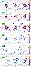 |
Fig. A.3. Cutouts of the X-ray detected AGN in the three protoclusters, in each band (soft, hard, full). Data are color coded by number of counts, while the green, blue and red contours are the extraction region, the prior position and the Lyα emission of the ELAN. |
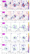 |
Fig. A.4. Cutouts of the X-ray detected AGN in the three protoclusters, in each band (soft, hard, full). Data are color coded by number of counts, while the green, blue and red contours are the extraction region, the prior position and the Lyα emission of the ELAN. |
Appendix B: X-ray spectra
We performed the spectral analysis using pyXspec (Gordon & Arnaud 2021) and report the results in Figure B.1. However, through the paper we use the results from this spectral analysis for sources with more than 30 counts in the full band.
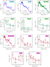 |
Fig. B.1. X-ray spectra of the AGN detected in the three protocluster. The solid lines are the fit performed using an unabsorbed power law. For sources with more than 30 net counts, the line represents the best fit, while for the other sources (J0819-16, J0819-24, Fab-21, Fab-33, Fab-41) is a power-law with Γ fixed to that found using the HRs. |
Appendix C: Slug optical photometry and SED fitting
C.1. Optical observations of the Slug protocluster
We obtained new optical images of the Slug protocluster with the Large Binocular Camera (LBC) instrument mounted on the Large Binocular Telescope (LBT) with the U_spec (51 min), BBessel (20 min), gSDSS (10 min), VBessel (15 min), rSDSS (15 min), iSDSS (15 min), zSDSS (37 min) filters. The reduction, astrometric and photometric calibration, and quality assessment of these data has been carried out at the LBC Survey Center5 in Rome, following standard LBC procedures and pipelines. We used the Graphical Astronomy and Image Analysis Tool (GAIA)6 and the Source-Extractor (Bertin & Arnouts 1996) software to perform source detection and produce photometric catalogs.
C.2. SED fitting properties of the Slug members
In this section, we investigate the main physical properties (e.g., stellar mass, star formation rate) of candidate protocluster members (i.e., galaxies in the prior catalogs without a spectroscopic confirmation of their redshifts) of the Slug, for which we have optical LBT observation in 7 filters (Uspec, BBessel, VBessel, iSLOAN, gSLOAN, rSLOAN, zSLOAN). In addition, for the two QSOs, we used the photometric points reported in Chen et al. (2021), i.e., FUV, NUV, J, H, Ks, W1, W2, W3, W4, 450 μm, 850 μm, 2 mm, 3 mm and 1.4 GHz. We derived such quantities through multiwavelength SED fitting, using the PYTHON “Code Investigating GALaxy Emission" (CIGALE; Boquien et al. 2019). Firstly, we performed a match between the 36,880 detected source in the LBT observations and the prior catalogs of 69 LAEs and SMGs available for the Slug protocluster. For the resulting 26 sources with a counterpart, we performed two separate CIGALE runs. One for the 2/26 members with an X-ray counterparts (i.e., the central QSO UM287 and the companion QSO, compQSO), including the X-ray and radio modules, since data in both band are present. The other run, for the remaining 24/26 sources, was performed without including the aformentioned modules, even though we used a similar input parameters set for the other SED components. In particular, we adopted a typical delayed SFH, combined with the Bruzual & Charlot (2003) module for the stellar component; we selected the Charlot & Fall (2000) module for the dust attenuation, along with the Draine et al. (2014) template for dust emission; finally, the AGN templates used are those from Stalevski et al. (2012, 2016) with the skirtor2016 module. In Figure C.1 the results from the SED fitting of the two QSOs are shown. Both sources SED is dominated by the AGN across the electromagnetic spectrum, which in turn did not allow us to put significant constraints on the main physical quantities related to the host galaxy. Indeed, both the stellar masses and SFRs of the two QSOs are poorly constrained by the SED fitting. The AGN parameters are instead well constrained by the fit. The companion QSO (compQSO), has a large AGN fraction (fAGN ∼ 0.85, defined as the ratio between the AGN and AGN + dust emission), and UM287 is dominated by the AGN contribution (fAGN ∼ 1).
For the Slug members, we mainly investigated their stellar masses and SFRs (averaged in 100 Myrs timescale, as provided by the CIGALE output), both obtained from the CIGALE output. Figure C.2 shows the main sequence (MS) of galaxies for these sources, along with a MS at the same redshift from Speagle et al. (2014). We also color-coded the points following their AGN fractions. Most of the galaxies are below the MS, even though some systematics may be present due to the SED fitting templates. We compare our results with those from the XMM-SERVS (Zou et al. 2022) at 2 < z < 2.5, which are slightly below the MS, but overall in agreement with our data points at the same stellar masses. CompQSO and UM287 are also displayed in the plot, with the former laying in the MS (log(SFR/SFRMS)∼ − 0.1) and the latter being quite offsetted (log(SFR/SFRMS)∼ − 0.3). However, the results may be significantly affected by the large uncertainties on those values.
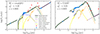 |
Fig. C.1. Best-fit SEDs of the central QSO (UM287) and companion QSO (CompQSO) in the Slug nebula. The best-fit model is shown in gray, while the individual contribution for each templates are shown in different colors: in green we show the AGN emission; the dust emission is displayed in orange; the stellar unattenuated and attenuated models are the dotted blue and solid yellow lines; the radio emission is highlighted in purple. Points and upper limit are shown as empty light-blue circles and red filled triangles, respectively. |
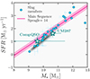 |
Fig. C.2. Main sequence of galaxies for the members of the Slug proto-. The azure circles are the member galaxies. The white stars are instead the two QSOs. The gray contours are the points from the XMM-SERVS (Zou et al. 2022). Finally, the magenta line represents the MS by Speagle et al. (2014) a z ∼ 2.2, plotted as a reference. |
All Tables
Properties of the X-ray detected AGN in the three protoclusters with number of counts > 30, derived from spectral analysis.
Properties of the X-ray-detected AGN in the three protoclusters derived using their HR.
All Figures
|
Fig. 1. Intrinsic 2 − 10 keV luminosity versus column density. Protocluster members are shown in cyan, magenta, and green. Diamonds indicate sources whose properties were derived via spectral fitting, while circles are for sources with properties derived from their hardness ratio (HR). Other classes of AGN detected in the X-ray are shown in different colors (Urrutia et al. 2005; Just et al. 2007; Wang et al. 2013; Banerji et al. 2014; Stern et al. 2014; Assef et al. 2016; Corral et al. 2016; Martocchia et al. 2017; Mountrichas et al. 2017; Ricci et al. 2017; Goulding et al. 2018; Vito et al. 2018a; Zappacosta et al. 2018; Li et al. 2019; Lansbury et al. 2020; Zou et al. 2020). Newly discovered AGN (i.e., not known as such prior to this work) are highlighted with thick black circles. |
| In the text | |
|
Fig. 2. X-ray maps in the 1 − 2 keV band of the central QSOs of the Slug, Fabulous, and J0819 protoclusters (upper panels) with Lyα contours in white. Background-subtracted differential radial profiles for the emission surrounding the Slug (cyan), Fabulous (magenta), and J0819 (green) central QSOs are shown in the bottom panels, with respect to the PSF prediction (purple line). The secondary y-axis is based on the apec model with a fixed temperature of 2 keV. |
| In the text | |
|
Fig. 3. Fractions of X-ray-selected AGN among different population of galaxies (i.e., SMGs and LAEs) in the Slug, Fabulous and J0819 protoclusters, compared to other protoclusters (Lehmer et al. 2009; Digby-North et al. 2010; Smail et al. 2014; Chen et al. 2016; Macuga et al. 2019; Umehata et al. 2019; Vito et al. 2020; Polletta et al. 2021; Tozzi et al. 2022a; Monson et al. 2023; Pérez-Martínez et al. 2023; Vito et al. 2024; Travascio et al. 2025) and the X-ray AGN fractions in local clusters (Martini et al. 2006; Bufanda et al. 2017). Empty blue and green points indicate the fractions computed for spectroscopically confirmed members (see Table 5). |
| In the text | |
|
Fig. 4. X-ray luminosity functions in two different redshift bins (z ∼ 2.2 and z ∼ 3.2) and in luminosity bins of 0.5 dex. Our data are shown as cyan and green points, with different markers representing different assumptions on the co-moving volume. For comparison, XLFs for the field environment at similar redshifts are also reported. The solid purple line shows the XLF for field AGN from Gilli et al. (2007). The dashed lines correspond to the XLFs from Ueda et al. (2014) at z ∼ 2.2 and z ∼ 3.2. The dotted line shows the XLF from Georgakakis et al. (2015), and the purple shaded area represents the XLF estimated by Vito et al. (2018b). |
| In the text | |
|
Fig. 5. Cumulative space density in two redshift bins (z ∼ 2.2 and z ∼ 3.2). Our data are shown as a cyan point and a green shaded area, where the uncertainties are computed according to Gehrels (1986). For comparison, the cumulative space densities of other protoclusters at similar redshifts are also reported. The gray shaded region (left panel) represents the cumulative space density for the Spiderweb protocluster (see Tozzi et al. 2022a; Travascio et al. 2025), while the red and pink shaded areas (right panel) correspond to the MQN01 and SSA22 by Travascio et al. (2025). The purple solid line shows the cumulative space density for field AGN from Gilli et al. (2007). |
| In the text | |
|
Fig. 6. Left panel: Ratio of the number density of objects in the three protoclusters to that in the field, for AGN (stars) and SMGs (circles). Errors are computed in the Poissonian assumption. The environment of AGN with respect to field in our targets is 1–2 dex larger than overdensity of the parent population of galaxies, impliying a direct environmental effect on the SMBH growth in these structures. We also show the ratios for other protoclusters at various redshifts (Tozzi et al. 2022a; Vito et al. 2020, 2024; Travascio et al. 2025). Right panel: Ratio of AGN to SMG overdensity, as a function of SMG overdensity (top) and redshift (bottom), for the same protoclusters. |
| In the text | |
|
Fig. 7. X-ray vs Lyα luminosity of the extended emission from the ELANe. Magenta, green, and cyan circles represent the Fabulous, J0819, and Slug nebulae, respectively. Blue and white points show SSA22 extended Lyα emission reported by Geach et al. (2009); orange circles represent extended Lyα emission around HzRGs from Reuland et al. (2003); pink circles and squares correspond to extended Lyα emission in the Boötes and GOODS-S fields, respectively (Yang et al. 2009; Nilsson et al. 2006); the red circle marks the Spiderweb extended Lyα nebula fromTozzi et al. (2022b), and the white circle marks the LAB from Daddi et al. (2021). The solid black line represents the 1:1 relation (Geach et al. 2009), while the dashed black line indicates the LX = 1000LLyα relation (Cowie et al. 1980; Bower et al. 2004). The purple region (lower left) corresponds to the scenario in which the main powering channel of the extended Lyα emission is gravitational cooling. The gray area (upper right), represents the region in which the cooling cannot be the fueling mechanism of the nebula. |
| In the text | |
|
Fig. A.1. Chandra X-ray maps (gray scale) of the three fields, centered on the aim point. The coverage of ancillary data is superimposed as colored contours (orange, blue, red and magenta for SCUBA-2, MUSE, ALMA and KECK I, respectively). |
| In the text | |
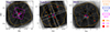 |
Fig. A.2. Same as Figure A.1 but for the exposure maps. |
| In the text | |
|
Fig. A.3. Cutouts of the X-ray detected AGN in the three protoclusters, in each band (soft, hard, full). Data are color coded by number of counts, while the green, blue and red contours are the extraction region, the prior position and the Lyα emission of the ELAN. |
| In the text | |
|
Fig. A.4. Cutouts of the X-ray detected AGN in the three protoclusters, in each band (soft, hard, full). Data are color coded by number of counts, while the green, blue and red contours are the extraction region, the prior position and the Lyα emission of the ELAN. |
| In the text | |
|
Fig. B.1. X-ray spectra of the AGN detected in the three protocluster. The solid lines are the fit performed using an unabsorbed power law. For sources with more than 30 net counts, the line represents the best fit, while for the other sources (J0819-16, J0819-24, Fab-21, Fab-33, Fab-41) is a power-law with Γ fixed to that found using the HRs. |
| In the text | |
|
Fig. C.1. Best-fit SEDs of the central QSO (UM287) and companion QSO (CompQSO) in the Slug nebula. The best-fit model is shown in gray, while the individual contribution for each templates are shown in different colors: in green we show the AGN emission; the dust emission is displayed in orange; the stellar unattenuated and attenuated models are the dotted blue and solid yellow lines; the radio emission is highlighted in purple. Points and upper limit are shown as empty light-blue circles and red filled triangles, respectively. |
| In the text | |
|
Fig. C.2. Main sequence of galaxies for the members of the Slug proto-. The azure circles are the member galaxies. The white stars are instead the two QSOs. The gray contours are the points from the XMM-SERVS (Zou et al. 2022). Finally, the magenta line represents the MS by Speagle et al. (2014) a z ∼ 2.2, plotted as a reference. |
| In the text | |
Current usage metrics show cumulative count of Article Views (full-text article views including HTML views, PDF and ePub downloads, according to the available data) and Abstracts Views on Vision4Press platform.
Data correspond to usage on the plateform after 2015. The current usage metrics is available 48-96 hours after online publication and is updated daily on week days.
Initial download of the metrics may take a while.