| Issue |
A&A
Volume 701, September 2025
|
|
|---|---|---|
| Article Number | A126 | |
| Number of page(s) | 19 | |
| Section | Stellar structure and evolution | |
| DOI | https://doi.org/10.1051/0004-6361/202555467 | |
| Published online | 05 September 2025 | |
Enhanced mass loss of very massive stars: Impact on the evolution, binary processes, and remnant mass spectrum
1
SISSA, Via Bonomea 365, I–34136 Trieste, Italy
2
INAF – Osservatorio Astronomico di Padova, Vicolo dell’Osservatorio 5, Padova, Italy
3
Dipartimento di Fisica e Astronomia, Università degli studi di Padova, Vicolo dell’Osservatorio 3, Padova, Italy
4
Institut d’Astronomie et d’Astrophysique, Université Libre de Bruxelles, CP 226 – Boulevards du Triomphe, B 1050 Bruxelles, Belgium
5
INAF – Osservatorio Astronomico di Roma, Via Frascati 33, I-00040 Monteporzio Catone, Italy
6
INFN – Sezione di Trieste, I-34127 Trieste, Italy
7
Gran Sasso Science Institute (GSSI), L’Aquila (Italy), Viale Francesco Crispi 7, 67100 L’Aquila, Italy
8
INFN, Laboratori Nazionali del Gran Sasso, 67100 Assergi, Italy
⋆ Corresponding author: This email address is being protected from spambots. You need JavaScript enabled to view it.
Received:
9
May
2025
Accepted:
18
July
2025
Abstract
Very massive stars (VMS) play a fundamental role in astrophysics. Their powerful stellar winds, which dictate their evolution, supernovae, and fate as black holes (BHs), are a key uncertainty, as evidence suggests their mass-loss rates may exceed standard predictions. To address this, we investigated the effect of enhanced winds on the single and binary VMS evolution by implementing new stellar wind prescriptions in the stellar evolution code PARSEC v2.0 and in the binary population synthesis code SEVN. Our updated models are sensitive to the Eddington parameter (Γe) and the luminosity-to-mass ratio. We used them to simulate the VMS evolution from 100−600 M⊙ at the metallicity of the Large Magellanic Cloud (LMC) to model the VMS population in the Tarantula Nebula. Our results show that Γe-enhanced single-star tracks agree better with the observed VMS properties in the Tarantula Nebula than the standard wind models. When the most massive star in the region, R136a1, is explained via a single-star evolution, a lower limit on the initial mass of ≳300 M⊙ is required, regardless of the wind recipe used. We also show that binary stellar mergers offer another suitable formation channel that might lower the required initial mass limit by ∼100 M⊙. The choice of the wind treatment profoundly impacts the BH populations. Stronger winds yield smaller BHs, which inhibits the formation of objects above the lower edge of the pair-instability mass gap (∼50 M⊙). For merging binary BHs, enhanced-wind models predict more primary BHs above 30 M⊙ and enable secondary BHs between 30−40 solar masses, which is a range not found with standard stellar winds at the metallicity of the LMC. This study highlights the crucial role of stellar wind physics and binary interactions in the evolution of VMS and resulting BH populations. It offers predictions that are relevant for interpreting VMS observations and gravitational-wave sources.
Key words: binaries: general / stars: black holes / stars: evolution / stars: massive / stars: mass-loss / stars: winds / outflows
© The Authors 2025
 Open Access article, published by EDP Sciences, under the terms of the Creative Commons Attribution License (https://creativecommons.org/licenses/by/4.0), which permits unrestricted use, distribution, and reproduction in any medium, provided the original work is properly cited.
This article is published in open access under the Subscribe to Open model. This email address is being protected from spambots. You need JavaScript enabled to view it. to support open access publication.
1. Introduction
Stellar winds are one of the most influential drivers of the evolution of very massive stars (VMS), which are defined as stars with initial masses ≥100 M⊙. Their strong winds enrich the surrounding interstellar medium (ISM) chemically, inject energy into the environment, and ionize the surrounding matter. Stellar winds also play a key role in forming Wolf-Rayet stars (WR), which are peculiar evolved massive stars with thick winds and strong emission line spectra. Stellar winds, which are driven by radiation pressure, regulate the mass loss over the stellar lifetime. These winds directly influence the initial-to-final mass relation of stars, which links the mass at the zero-age main-sequence (ZAMS) with the final remnant mass.
A variety of mass-loss prescriptions for massive stars have been developed, including those by Castor et al. (1975), de Jager et al. (1988), Nugis & Lamers (2000), Vink et al. (2000, 2001, 2011), Gräfener & Hamann (2008), Gräfener et al. (2011), which are widely used in stellar evolution models. An accurate determination of the mass-loss rates of VMSs remains a major open question in astrophysics, however, particularly in regimes near the Eddington limit, where theoretical uncertainties are significant and observational constraints are few. In recent years, considerable effort has been made to constrain the relation between the initial and remnant masses of VMSs better. Driven by new observational data and advances in hydrodynamical modeling, updated mass-loss prescriptions are being introduced regularly (e.g., Bestenlehner 2020; Sabhahit et al. 2022; Björklund et al. 2023; Gormaz-Matamala et al. 2024). As a result, it is essential to implement and test these theoretical prescriptions in stellar evolution models to evaluate their impact on the structure and fate of VMSs.
The Tarantula Nebula (30 Doradus cluster) in the Large Magellanic Cloud (LMC) is a treasure trove of massive stars because it hosts the most massive single stars ever observed. Several of these stars have a M ≥ 100 M⊙ (Crowther et al. 2010; Bestenlehner et al. 2020; Brands et al. 2022; Shenar et al. 2023, hereafter, C10, B20, and B22, respectively). Observations showed that the effective temperatures of VMSs in the Tarantula Nebula fall within a relatively narrow range, 4.6 ≲ log (Teff [K]) ≲ 4.74 (C10; Bestenlehner et al. 2014; Schneider et al. 2018; B22; Crowther et al. 2016). A similar trend was observed in the Arches cluster, where VMSs lie in the range 4.5 ≲ log (Teff) ≲ 4.6 (Martins et al. 2008).
While this tight temperature distribution might be attributed to a recent burst of star formation, it poses a challenge to standard stellar evolution models, which predict that VMSs should undergo significant radius growth toward the end of the main sequence (MS). This envelope inflation occurs while the star is still in hydrostatic and thermal equilibrium, and it is driven by opacity effects in the outer layers, which are distinct from the post-MS expansion phase (Sabhahit & Vink 2025). This inflation would shift models to cooler effective temperatures than are currently observed in the Tarantula cluster and cause them to evolve toward large radii and lower Teff, potentially crossing the Humphreys-Davidson (HD) limit (Humphreys & Davidson 1979). This contradicts observations. Accurate inflation modeling remains highly uncertain and model dependent, however. Recent work suggested that the radial extension of VMS may originate from the simplified treatments of the stellar atmosphere in 1D evolution codes (Josiek et al. 2025).
Alternatively, revised and enhanced mass loss of VMSs remains a valid explanation to prevent this inflation and to reproduce the observed properties of VMSs more accurately to fix the discrepancy. A potential solution, proposed by Sabhahit et al. (2022), involves higher stellar wind mass-loss rates in a way that balances the effects of mass loss and envelope inflation, thereby allowing stars to maintain nearly constant effective temperatures during the MS. Because the evolution of VMSs in close proximity to the Eddington limit can be uncertain, even small changes in the mass-loss rate can significantly affect their evolutionary properties. Thus, adjusting the wind prescription in this regime might reconcile theoretical models with the observations.
Winds are not the only source of uncertainty in the VMS evolution, however. Binary interactions can be consequential in shaping the evolution and final outcomes of VMSs, which are frequently found in binary or multiple systems (Mason et al. 2009; Sana et al. 2013). About 70% of the massive stars exist in binary systems that will interact and exchange mass within their lifetime (Smith 2014, and references therein). They have a preference for massive companions (Kobulnicky & Fryer 2007). In this scenario, stellar winds play a pivotal role. For instance, a higher mass-loss rate can prevent a star from expanding to the red supergiant (RSG) stage (Smith 2014; Josiek et al. 2024), thus avoiding eventual mass-transfer episodes. Products of binary interactions have also been proposed as an explanation for various stellar objects, such as luminous blue variable stars (Gallagher 1989; Justham et al. 2014; Smith & Tombleson 2015) and long-lived blue supergiants (BSGs) (e.g., for the progenitor of SN1987A, Podsiadlowski et al. 1990; Menon & Heger 2017). Moreover, binary interactions can alter the physical appearance of stars; Roche-lobe overflow (RLOF) can strip a massive star of nearly its entire hydrogen envelope, making it resemble a WR star (Vanbeveren & Conti 1980; Petrovic et al. 2005). In some cases, stars in binary systems may even collide and merge to form a more massive star that continues the stellar evolution and can appear similar to a star that is born with a higher ZAMS mass (Portegies Zwart & McMillan 2002; Freitag et al. 2006; Costa et al. 2022). These wind-driven and binary interaction processes not only shape the evolution and final masses of VMSs, but also influence the formation of compact object binaries. In particular, binary systems with massive stars can ultimately evolve into black hole (BH) binaries, which may merge within a Hubble time and produce gravitational-wave signals that are detectable by current observatories (Abbott et al. 2016).
We introduce newly implemented wind prescriptions in the PARSEC v2.0 stellar evolution code, which are designed to capture the enhanced mass-loss behavior of VMSs near the Eddington limit, following Sabhahit et al. (2022). The prescriptions were not previously included in the code and enable us to explore how stronger wind dependencies affect the evolution of VMSs. As a testbed, we focus on the Tarantula Nebula in the LMC, whose rich population of massive stars, especially in the R136 cluster, offers valuable observational constraints. We compute the stellar evolution tracks for single stars across a wide initial mass range (100−600 M⊙) at the LMC metallicity. For the first time, we integrate these updated tracks into the binary population synthesis code SEVN. This allows us to systematically explore the effect of stronger winds on the single and binary evolution of VMS, including their remnant masses and the formation pathways of merging BHs. Our aim was to address key uncertainties in the mass-loss behavior of VMSs, to evaluate whether the models can reproduce the observed stellar properties in the Tarantula Nebula, and to assess their implications for the population of gravitational-wave sources at LMC-like metallicity.
The paper is organized as follows. We describe the observational data, the input physics of our stellar tracks, and the setup of our binary population synthesis simulations in Sect. 2. In Sect. 3 we present the single stellar evolution models with the new wind implementation. We discuss their evolution on the Hertzsprung-Russell diagram (HRD) in Sect. 3.1, their chemical evolution in Sect. 3.2, and the pre-supernova (pre-SN) and BH masses in Sect. 3.3. In Sect. 4 we explore the effects of strengthened winds on binary stellar evolution. In Sect. 4.1 we discuss stellar wind accretion in binaries, and we describe stellar mergers in Sect. 4.2 and the resulting BH mass distribution in Sect. 4.3. Then, in Sect. 5, we discuss the implications, applicability, and uncertainties of our models and results. Finally, our results are summarized in Sect. 6.
2. Methods
2.1. Observational data
The primary focus of this study is on VMS, and we therefore focused our analysis on R136, a concentration of stars in the NGC 2070 star cluster located in the Tarantula Nebula. Initial studies suggested that the central object in R136 is a single star with a mass > 1000 M⊙ (Cassinelli et al. 1981; Savage et al. 1983). Follow-up studies showed, however, that the central region is instead comprised of distinct stellar sources (Weigelt & Baier 1985; Lattanzi et al. 1994). Even as individual stars, the central region still hosts the most massive stars known to date, with current mass estimates of ∼150−300 M⊙ (C10). In particular, it hosts three stars (R136a1, R136a2, and R136a3) with masses above ∼150 M⊙, cataloged as WNh type, that is, rare WR of nitrogen type (WN) that show hydrogen lines in their spectra, and are likely still undergoing core-hydrogen burning (Massey & Hunter 1998; de Koter et al. 1998; Smith & Conti 2008).
The LMC metallicity is estimated to be between a quarter and half of that of the Sun ([Fe/H] ≃ −0.37 to [Fe/H] ≃ −0.41) (Choudhury et al. 2016, 2021) and stellar modelers frequently use Z ≃ 0.5 Z⊙ (i.e., Z ≈ 0.006) when simulating stars in the Tarantula Nebula (Bestenlehner et al. 2014; Schneider et al. 2018; B22; Martinet et al. 2023; Josiek et al. 2024).
We compare our models with data from Schneider et al. (2018), which comprises more than 400 stars in the 30 Doradus region, obtained from the VLT-FLAMES Tarantula Survey (Evans et al. 2011). These data were obtained using the Hubble Space Telescope and the Multi Unit Spectroscopic Explorer (MUSE) on the Very Large Telescope (VLT) and contain a compilation of results from Bestenlehner et al. (2014), Sabín-Sanjulián et al. (2014, 2017), McEvoy et al. (2015), Ramírez-Agudelo et al. (2017). We also compare our models with data from B22 of the central regions of the R136 star cluster taken with the Hubble Space Telescope/STIS (Crowther et al. 2016). The raw spectroscopic data from VLT and HST required nontrivial steps in data reduction and analysis to obtain effective temperatures and luminosities. The process involves fitting stellar atmosphere models, which themselves carry uncertainties. B22 provides the best fit parameters and 1σ error bars for the optical + UV fits of 39 stars with high S/N.
Figure 1 shows the HRD of tracks using the standard mass-loss recipe from Costa et al. (2025) and stellar data from Schneider et al. (2018) and B22. The figure shows excellent agreement between the data and the evolutionary tracks for stars with ZAMS masses ≲80 M⊙, as the ZAMS and terminal-age main sequence (TAMS1) of the tracks effectively bracket the observed stars. More massive stars show a different picture: assuming that these stars are all part of the same starburst, the width between the ZAMS and TAMS in the stellar models is significantly broader than suggested by the data, and, at the TAMS, the models are cooler than the observed ones (4.75 ≤ log (Teff [K]) ≤ 4.6). The discrepancy can be alleviated with very young ages of the cluster (< 1 Myr), where stars populate only the hotter side of the MS, rapid rotation, or with increased mass-loss rates, which can suppress the occurrence of envelope inflation. Such a young age seems unlikely, as stars would still retain their H envelope and would not yet appear as WNh. Additionally, various studies have suggested older stellar ages of 1−2.5 Myr (C10; B20). The VMS observed are not rapidly rotating (Bestenlehner et al. 2014; B20), and VMS are not largely affected by moderate rotational mixing (Yusof et al. 2013). For these reasons, we investigate an alternative enhanced wind prescription with increased mass-loss to explain this observed feature of VMS.
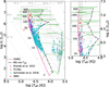 |
Fig. 1. Hertzsprung-Russel diagram adapted from Costa et al. (2025) showing stars in the LMC. The green and gray lines show tracks from Costa et al. (2025), that were computed with Z = 0.006 and the standard mass-loss rate. The purple and red stars show objects from B22 (red stars indicate R136a), and the blue and red dots are taken from Schneider et al. (2018) (red dots are WNh stars). The dashed pink line and dash-dotted black line show the ZAMS and TAMS, respectively. The zoomed-in plot shows the most massive stars, and the gray shaded region shows the width of the observed temperature range of VMSs in the LMC. |
2.2. Bayesian statistical analysis
We used an updated version of the PARAM2 code (da Silva et al. 2006; Rodrigues et al. 2014, 2017), which will be soon released (Bossini et al., in prep.), to fit the observed data with our stellar tracks (described in the following section). The code exploits Bayesian statistics, using the observed abundances, effective temperature, and luminosities (and their uncertainties) to estimate stellar parameters of interest, like age, initial and current mass, and log g, using theoretical isochrones derived from our stellar evolutionary tracks. The output of PARAM gives the best fitting value with its correlated error, that is, the associated credible intervals that include 68% of the distributions.
2.3. Stellar code and input physics
We present new stellar evolution tracks computed with the PAdova and TRieste Stellar Evolution Code (PARSEC, Bressan et al. 2012) v2.0 with new mass-loss implementations for VMS. PARSEC v2.03 has been described in detail by Costa et al. (2021, 2025), Nguyen et al. (2022), and PARSEC v1.2 in previous works (Chen et al. 2015; Fu et al. 2018). Below, we provide a brief summary of the main input physics used in the code.
The stellar tracks evolve from the pre-main sequence (PMS) to either the oxygen-burning stage or until entering the dynamical electron-positron (e+–e−) pair instability (PI) regime (Heger & Woosley 2002). To determine when the stars become dynamically unstable, PARSEC uses the criterion of Stothers (1999), which provides a good approximation for assessing stellar stability without requiring detailed hydrodynamical simulations. At each time step, we compute the volumetric pressure-weighted average of the first adiabatic exponent, ⟨Γ1⟩, and stop the evolution if it goes below 4/3. To be conservative, we consider the star dynamically unstable when ⟨Γ1⟩ < 4/3 + 0.01 (as suggested from dynamical investigations by Marchant et al. 2019). This method to identify when the star enters the PI regime has already been adopted in previous works (Costa et al. 2021, 2022, 2025; Volpato et al. 2023, 2024). We compute nonrotating4 tracks with initial masses 100 ≤ MZAMS/M⊙ ≤ 600 with a mass step of 10 M⊙ for tracks with 100 ≤ MZAMS/M⊙ ≤ 400, and a mass step of 50 M⊙ above. We focus on this mass range to investigate the effect of enhanced stellar winds of VMS near the Eddington limit, since stars with smaller initial masses do not approach the Eddington limit until much later in evolution.
Stellar tracks are computed with metallicity Z = 0.006 and Y = 0.259 in mass fraction (i.e., [M/H] = −0.4045), to investigate the massive-star hosting environment of the LMC. We adopt the solar-scaled mixtures from Caffau et al. (2011) and take the solar metallicity to be Z⊙ = 0.01524.
Energy transport via convection is described using the mixing length theory (Böhm-Vitense 1958). We set the mixing length parameter αMLT = 1.74 (as suggested by Bressan et al. 2012). We test stability against convection using the Schwarzschild criterion (Schwarzschild 1958).
Core overshooting is included in our calculations, which allows for convective elements to penetrate into stable regions6. The overshooting parameter is set to λov = 0.5 in pressure scale height, HP, which indicates the maximum distance an overshooting bubble can travel across the unstable border. Therefore, in our framework the overshooting length is then lov ≈ 0.5λovHP = 0.25HP. Overshooting from the convective envelope is also taken into account, extending from the base of the convective envelope downward by Λenv = 0.7HP.
The stellar type is tracked throughout the evolution of the star and is determined by its burning phases, surface abundances, and Teff. The definitions of the stellar types referenced in this work are listed in Table 1.
Definitions used for different stellar types, adapted from Josiek et al. (2024).
2.4. Mass-loss descriptions
2.4.1. Standard winds
This section outlines the mass-loss prescriptions implemented in our models. The standard mass-loss rate for massive stars (MZAMS ≥ 10 M⊙) used in PARSEC v2.0 is the same as that used in previous works (Chen et al. 2015; Volpato et al. 2023, 2024; Costa et al. 2025). This recipe is based on the prescription formulated by Vink et al. (2001), which provides the mass-loss rate as a function of stellar parameters for massive O and B type stars for a range of metallicities and temperatures. For hot stars (Teff ≥ 10 000 K), the main dependencies are
 (1)
(1)
where L, M, and Z are the current luminosity, mass, and metallicity of the star. The full equations are given in Vink et al. (2001), and also include a dependence on Teff and terminal velocity ν∞.
To account for the increase in mass-loss due to recombination or ionization of iron at different temperatures (i.e., the bistability jump), we adjust the mass-loss rate as described in Vink et al. (2001). We also account for the increase in mass-loss rates when the Eddington limit is approached (Gräfener & Hamann 2008) by using a fit to the models of Vink et al. (2011). The electron scattering Eddington parameter is calculated as:
 (2)
(2)
where κe is the opacity due to electron scattering, G is the gravitational constant, and c is the speed of light. The mass-loss rates follow different dependencies for high- and low-Γe regimes. For the high-Γe regime, the dependencies are given as (Vink et al. 2011)
 (3)
(3)
For cool RSG and YSG stars (Teff < 10 000 K) we take the maximum between the Vink et al. (2001) rates and the rates provided by de Jager et al. (1988). For WR stars, defined here as those with relative surface hydrogen abundance < 0.3, we apply the luminosity-dependent mass-loss prescription from Sander et al. (2019),
 (4)
(4)
which is adjusted to include a metallicity dependence based on Vink (2015). The combination of the above mass-loss recipes are referred to as Ṁrdw (radiation driven winds) for simplicity and to keep consistency among other works (Volpato et al. 2023, 2024), however we acknowledge that other mass-loss mechanisms may be as work, like in RSGs.
2.4.2. New winds for VMSs
Sabhahit et al. (2022) proposed enhanced mass-loss rates for VMS transitioning from O-type to WNh stars based on theoretical and observational evidence, marking a shift from optically thin to optically thick winds. The proposed rates use the so-called transition mass-loss rate, which is a model-independent mass-loss rate that describes the transition from O to WNh winds. The transition mass-loss rate is given as
 (5)
(5)
where f is a metallicity dependent correction factor, f = 0.6 (Vink & Gräfener 2012). One can use the average values of luminosities and terminal velocities of observed Of/WNh stars to calculate the Γe, trans, which is the location of the upturn in mass-loss rates. By computing the Ṁtrans, a model-independent transition mass-loss rate is obtained in which the winds switch from optically thin to optically thick when above the transition point. Sabhahit et al. (2022) empirically obtained the transition parameters of the Of/WNh stars in the Tarantula Nebula to be L/L⊙ = 106.31, ν∞ = 2550 km/s, log Teff = 4.64, and Xs = 0.62. For the LMC, the location of the increase in mass-loss is thus calculated to be Γe, trans = 0.42, and the transition mass-loss rate is log Ṁtrans = −5.0 (Sabhahit et al. 2022). The main dependencies for the enhanced winds of VMS are given as
 (6)
(6)
 (7)
(7)
where  is the surface hydrogen abundance (in mass fraction), included only in the ṀSab, Γe recipe. The ṀSab,L/M recipe omitting a surface
  dependence is an extreme case, used to show that the L/M has a larger effect on the mass-loss rates than the
  , and the
  dependence may not be strictly necessary, like the recipe of Eq. (1). The full recipes are given in Equations (12) and (13) in Sabhahit et al. (2022). Our models adopt two variations, which we refer to as ṀΓe and ṀL/M:
 (8)
(8)
 (9)
(9)
Choosing the maximum of the Vink et al. (2001) and the Sabhahit et al. (2022) recipes automatically uses the low-Γe recipe (ṀVink01) below the transition point and switches to the high-Γe recipe of ṀSab, Γe and ṀSab,L/M above it. For each wind recipe, we ran a total of 35 stellar evolution tracks of VMS with initial masses between 100 and 600 M⊙.
2.4.3. Differences in the wind prescriptions
To illustrate the main differences in the mass-loss treatment, Figure 2 shows the mass-loss predictions for different recipes and stellar parameters7. The values were computed for a fixed Z, Teff, and νinf. All the Ṁ values increase with increasing luminosity. Smaller surface H abundances (at the same metallicity) decrease the mass-loss rates for the ṀVink11 and ṀSab, Γe predictions, while they do not affect the ṀVink01 or ṀSab,L/M ones, as they have no dependence on  . The ṀSab, Γe and ṀSab,L/M rates show a similar trend when
  , but begin to diverge with decreasing
  .
.
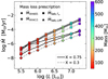 |
Fig. 2. Mass-loss rates predicted for different prescriptions as a function of the mass and luminosity for two |

As the luminosity increases, the ṀVink11 surpasses the ṀVink01 around log L/L⊙ ∼ 7.0, (depending on the  ) due to the star approaching the Eddington limit. Similarly, the ṀSab, Γe and ṀSab,L/M rates are greater than the ṀVink01 rates only when log L/L⊙ ≳ 6.25, (i.e., entering the high-Γe regime). The ṀSab, Γe and ṀSab,L/M rates are always greater than the ṀVink11 rate at log luminosities ≥5.5, but follow a similar trend.
2.5. Binary evolution with SEVN
To investigate the influence of different mass-loss on the evolution of binary populations, we used the state-of-the-art population synthesis code Stellar Evolution for N-body (SEVN, Spera et al. 2015, 2019; Spera & Mapelli 2017; Iorio et al. 2023). SEVN8 is a highly flexible tool for population synthesis, utilizing on-the-fly interpolation of pre-computed stellar evolution tracks, making it both efficient and adaptable for different evolutionary scenarios. To study the effect of the new stellar winds prescriptions on the distributions of the final binary compact objects, we used the TRACKCRUNCHER9 tool to adopt the new stellar evolutionary tracks with different winds to include in SEVN. For stars with masses MZAMS < 100 M⊙, we use the stellar models from Costa et al. (2025) with standard stellar winds, while for stars with MZAMS ≥ 100 M⊙, we use the new models presented in this paper. SEVN includes various prescriptions accounting for both the final supernovae (SN) type of massive stars, such as core-collapse supernovae (CCSN), pulsational pair-instability supernovae (PPISN), and pair-instability supernovae (PISN), and binary stellar evolution processes (e.g., Roche-lobe overflows, common-envelope phases, and SN kicks). Wind mass transfer is taken into account self-consistently, and the mass accretion rate depends on the wind mass-loss rate of the donor star, the mass of the donor and accretor, wind velocity, characteristic orbital velocity, effective radius, semimajor axis, and eccentricity (for more details, see Iorio et al. 2023). In this work, we use the standard SEVN code configuration, in its version 2, as extensively described by Iorio et al. (2023).
To determine the final fate of massive stars, we employ the delayed model for CCSN from Fryer et al. (2012), while for the PPISN and PISN regimes, and direct BH collapse (DBH), we use the formalism from Spera & Mapelli (2017), Mapelli et al. (2020). For the treatment of binary stellar evolution processes, we rely on the fiducial choices by Iorio et al. (2023), such as common envelope (CE) efficiency α = 1, mass transfer efficiency fMT = 0.5, and the standard treatment for the stability of mass transfer events is determined as in Hurley et al. (2002), with the addition that mass transfer is assumed to always be stable for donor stars with radiative envelopes.
To create our population of binary stars, we generate the initial conditions as follows. For each binary system, the mass of the primary star is extracted from a Kroupa (2001) initial mass function (IMF). We specifically sample masses ranging from 20 to 350 solar masses (M⊙) to focus on the effects of massive star winds on the spectrum of remnant masses. Thus, we obtain the mass of the primary star MZAMS, 1 as
![Mathematical equation: $$ \begin{aligned} \mathrm{pdf}(M_{\mathrm{ZAMS},\,1})\propto M_{\mathrm{ZAMS},\,1}^{-2.3} \quad \mathrm{with}\; M_{\mathrm{ZAMS},\,1} \in [20, 350]. \end{aligned} $$](/articles/aa/full_html/2025/09/aa55467-25/aa55467-25-eq27.gif) (10)
(10)
We extract the binary properties following the distributions presented in Sana et al. (2012). Therefore, the mass ratio q is extracted as
![Mathematical equation: $$ \begin{aligned}&\mathrm{pdf}(q)\propto q^{-0.1} \quad \mathrm{with}\; q = \dfrac{M_{\mathrm{ZAMS},\,2}}{M_{\mathrm{ZAMS},\,1}} \in [q_{\rm min}, 1.0] \end{aligned} $$](/articles/aa/full_html/2025/09/aa55467-25/aa55467-25-eq28.gif) (11)
(11)
 (12)
(12)
where MZAMS, 2 is the mass of the secondary star, and it is determined simply as
 (13)
(13)
Finally, the initial orbital periods P and eccentricities e are sampled as
![Mathematical equation: $$ \begin{aligned} \mathrm{pdf}(\mathcal{P} ) \propto \mathcal{P} ^{-0.55}, \quad \mathrm{with}\; \mathcal{P} = \log (P/\mathrm{day}) \in [0.15, 5.5] \end{aligned} $$](/articles/aa/full_html/2025/09/aa55467-25/aa55467-25-eq31.gif) (14)
(14)
and
![Mathematical equation: $$ \begin{aligned} \mathrm{pdf}(e) \propto e^{-0.42}, \quad \mathrm{with}\; e\in [0, 0.9]. \end{aligned} $$](/articles/aa/full_html/2025/09/aa55467-25/aa55467-25-eq32.gif) (15)
(15)
We generated an initial population of 107 binaries at the ZAMS and used them as initial conditions for all of our simulations. Each population utilizes the same treatments for binary evolution processes and final fates described above. Such populations are then evolved with the three different sets of stellar tracks computed with the various mass-loss recipes presented in Sect. 2.4, to study the effect of different stellar winds prescriptions on the evolution of stellar binaries.
3. Results from the single-star evolution
3.1. Evolution on the HRD
Figure 3 shows the HRD of selected tracks computed with the three different mass-loss recipes at LMC metallicity. The evolution of the star with MZAMS = 150 M⊙ shows a fairly similar evolution on the MS despite different mass-loss treatments. We find a similar behavior for stars with initial masses below 150 M⊙. They all increase in luminosity and move to lower Teff, with the Ṁrdw track evolving at slightly higher luminosity than those using other mass-loss rates. The similar evolution arises because these models do not enter the high-Γe regime on the MS. Therefore, they have mass-loss rates similar to the standard rates of Ṁrdw (before reaching a bistability jump). The greatest difference occurs after the MS. The Ṁrdw ignites core-helium burning (CHeB10) at cooler Teff than the other models, as a yellow supergiant (YSG). Meanwhile, the ṀΓe and ṀL/M tracks ignite CHeB as WN stars, near log Teff 4.5−4.6.
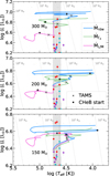 |
Fig. 3. Hertzsprung-Russel diagram showing the evolution of stellar tracks computed with the Ṁrdw, ṀΓe, and ṀL/M winds in blue, green, and pink, respectively. The models are shown with ZAMS masses of 300 M⊙ (top), 200 M⊙ (middle), and 150 M⊙ (bottom). The data symbols and shaded gray area are the same as in Figure 1. The black crosses and dots indicate the model location at the TAMS and the start of CHeB. The diagonal dashed gray lines show constant stellar radii as labeled. |
At larger MZAMS, more significant differences in the evolutionary paths begin to emerge. As can be seen in the comparison of 200 and 300 M⊙ stellar tracks, the ṀΓe and ṀL/M tracks encompass a narrower Teff range on the MS when compared to the Ṁrdw tracks. At the start of the MS, the ṀΓe models show a slight luminosity decrease and then evolve to cooler Teff. Then, they become WNhs shortly before reaching the bistability jump at log Teff ≃ 4.4, where the mass-loss rate increases and the track moves to higher Teff. The jump is also experienced by the Ṁrdw models here. The evolution of the 200 and 300 M⊙ tracks is markedly different when computed with the ṀL/M rates. These tracks show a sharp decrease in luminosity early on the MS and continue to evolve nearly vertically until just before the end of the MS. This vertical evolution is a result of the high mass-loss rates causing the stellar luminosity to decrease, which has a self-regulatory effect: it reduces the mass-loss rates (preventing quickly stripping the star and evolving to hotter Teff) and suppresses envelope inflation (thus preventing the star from becoming cooler). This balance between these two competing effects could provide a natural way to account for the observed constant temperatures of VMS in the Tarantula Nebula. These ṀL/M tracks become WNh stars earlier than the other two tracks, and spend up to 30% of the MS as WR stars. To provide a complete picture of the MS evolution, in Table 2, we present the TAMS masses for several initial masses. For increasing ZAMS mass, the enhanced wind models have stronger mass-loss rates, resulting in a greater divergence from the standard model masses.
Top table: TAMS mass for each mass-loss rate for a few initial masses. Bottom table: Time spent in the observed temperature range log Teff between 4.75 and 4.6.
We find that stellar tracks computed with the ṀΓe and ṀL/M winds spend more time in the observed Teff region and inflate less compared to the Ṁrdw tracks. Depending on the ZAMS mass, the tracks with enhanced winds can even evolve vertically down on the MS, due to the balance between mass-loss rate and envelope inflation. Table 2 lists the cumulative time spent within the Teff range of observed VMS transitioning to the WNh sequence. Models with Ṁrdw spend < 1 Myr in the observed limits, ṀΓe models spend ∼1.6 Myr within the range, and ṀL/M models spend from 1.2−2.1 Myr within the limits.
Given that the R136 cluster is estimated to be between 1−2.5 Myr old, and the individual stars in R136a are estimated to have ages of approximately ∼1−1.7 Myr (C10; B20; B22), tracks with Ṁrdw would be too cool to match the data unless the stars were very young (< 1 Myr). In comparison, the ṀΓe and ṀL/M models spend most of their lives within the observed ranges. Thus, the ṀΓe and ṀL/M models can better reproduce the observed VMS properties in the R136 star cluster than the Ṁrdw models.
To further investigate this aspect, we perform a fitting procedure exploiting the PARAM statistical tool (described in Sect. 2.2) to fit the three most massive stars of the cluster (namely, R136a1, R136a2, and R136a3) with our stellar tracks with initial masses up to 400 M⊙ with standard and new winds prescriptions. As input values, we adopt the current luminosity and effective temperature of stars provided by B22, and choose a fixed metallicity abundance of [Fe/H] = −0.404. As output of the fitting procedure, we obtain the stellar parameters listed in Table 3, that is, the initial mass, the current mass, and the age of the three stars for each wind recipe. The analysis shows that stellar evolutionary tracks calculated using the Ṁrdw and ṀL/M wind prescriptions predict ages for the three stars that are consistently too young. In contrast, the tracks computed with ṀΓe yield ages that align very well with the cluster age reported by other studies (C10; B20; B22) This analysis emphasizes that ṀΓe is the most effective wind prescription for modeling the VMS WNh stars in the R136 cluster in terms of ages, luminosities, and effective temperatures.
Best fit of the stellar tracks within the 68% confidence interval for the massive stars R136a1, R136a2, and R136a3.
Our results establish a strict lower limit on the possible initial mass for R136a1 in the single-star scenario, since no models with an initial mass below 300 M⊙ fit the data within the uncertainty. These results are in line with other works that estimate the mass of R136a1: C10 found the initial mass to be 320 M⊙, while B22 found Mini = 273
 M⊙. For R136a2, all of our predictions for the initial mass are in agreement with C10, who suggested 240
 M⊙, while our initial mass suggestions are slightly larger than B20 and B22, who provided an initial mass of 211
 M⊙ and 221
 M⊙, respectively. Finally, all of our derived initial masses for R136a3 are larger than suggested by other authors, who give 165
 M⊙ from C10 and 181
 M⊙ from B20, and 213
 M⊙ from B22. The derived initial and current masses for R136a2 and R136a3 are listed in Table A.1 in Appendix A. This discrepancy arises due to the different stellar models employed and different treatments for the mass-loss. C10 used GENEVA tracks (Eggenberger et al. 2008), while the more recent works used BONN stellar tracks (Brott et al. 2011; Köhler et al. 2015) and the BONNSAI Bayesian tool (Schneider et al. 2014). Additionally, each work has different assumptions for the mass-loss: C10 and B22 take wind clumping into account while B20 assumes smooth wind. The offset between our results and other authors for the initial masses suggests that our mass-loss rates are stronger, thereby requiring a larger initial mass to reproduce the present-day luminosity.
Our derived stellar ages for R136a show the best agreement with other estimates from literature for the tracks computed with the ṀΓe wind prescription. Specifically, these derived ages are slightly older than those provided by B22, but remain within their reported uncertainty. Similarly, our stellar ages are slightly younger than the age estimates from C10, which also fall within their uncertainty. In contrast, using the Ṁrdw and ṀL/M prescriptions results in much younger derived ages, less than 1 Myr, which is inconsistent with the ages reported in other studies.
Figure 4 shows the maximum radii reached during the MS and the whole lifetime for the different mass-loss rates as a function of the initial mass. The stellar tracks with ṀL/M have the smallest radii, as they lose their outer envelope and large fractions of mass early in the evolution. Consequently, they typically do not expand during shell-burning phases, unlike other tracks. Indeed, these tracks with ṀL/M and MZAMS ∼ 160 − 350 M⊙ have maximum radii reached during the MS and are near their ZAMS radius, about tens to 100 R⊙. Meanwhile, the stellar tracks with Ṁrdw and ṀΓe reach their maximum radii in the post-MS phases. Tracks with Ṁrdw and ZAMS masses below ∼200 M⊙ generally reach their maximum radii of ∼500−1000 R⊙ at the start of the CHeB phase. Similarly, tracks with ṀΓe and MZAMS ≤ 130 M⊙ reach their maximum radii of ∼1000 of R⊙ at the start of CHeB. For larger masses of both sets, the maximum radius is reached only during the final phase of evolution, when the star quickly crosses the HRD in a timescale as short as just a few years. The Ṁrdw tracks reach ∼700−1000 R⊙ in this stage, while the ṀΓe tracks similarly reach ∼500−1000 R⊙. This final stage is uncertain, as the timescales are very short and may depend on the numerical and physical atmosphere details. In both cases the maximum radius reached on MS and after, show that: Rmax(ṀL/M) < Rmax(ṀΓe) ∼ 102 R⊙ < Rmax(Ṁrdw). The time spent at larger radii directly influences the likelihood and type of binary interactions, as discussed in Sect. 4.1.
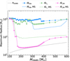 |
Fig. 4. Maximum radius reached for each ZAMS mass for tracks computed with different mass-loss rates, indicated by the color and marker. The solid lines with blue circles, green diamonds, and pink stars show the maximum radius reached during the evolution for tracks computed with Ṁrdw, ṀΓe, and ṀL/M winds, respectively, and the dashed lines show the maximum radius reached on the MS. The dashed ṀL/M is superimposed on the solid line. The solid gray line shows the ZAMS radius. |
3.2. Structure and chemical evolution
Figure 5 shows the Kippenhahn diagrams for three different mass-loss rates of a MZAMS = 200 M⊙ stellar track. The differences in the mass-loss rates are most pronounced during the MS, where stars spend most of their life. As mentioned above, all of these tracks become WRs on the MS. The ṀL/M track is the first to become a WNh at t = 1.83 Myr, as the stronger winds peel off the star’s H envelope faster than the other two wind prescriptions. The enhanced wind strength of ṀΓe and ṀL/M stellar tracks result in a smaller H burning region by the end of the MS, producing smaller He cores, (defined as the mass coordinate where XH < 10−3) compared to the case of standard winds. By the end of the MS, the Ṁrdw star has lost 80 M⊙ of material, the ṀΓe one has lost 100 M⊙, and the ṀL/M has lost 130 M⊙ of its material due to stellar winds.
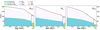 |
Fig. 5. Kippenhahn diagrams of the stellar tracks computed with the three mass-loss rates with MZAMS = 200 M⊙. The solid blue and green regions show the H and He burning zones, and the purple hatched region shows convective zones. The solid black and navy lines indicate the total mass and the mass of the He core. The red square indicates when the star enters the WR phase (i.e., when |

In the post-MS phases, tracks with Ṁrdw tend to expand, becoming YSGs before igniting CHeB (as shown in Figure 3). In contrast, the tracks computed with the new winds ignite CHeB at higher Teff, typically as WN stars. All 200 M⊙ models have a small envelope at the start of CHeB. The ṀΓe model is the only one that maintains a He-rich envelope throughout its evolution, while the other models lose it and expose their bare cores at the end of evolution. In general, ṀΓe and ṀL/M tracks stay hotter than the Ṁrdw one for the remainder of the evolution.
The stellar wind prescriptions not only affect the structural evolution of stars described above but also influence the abundances and nucleosynthetic products. Figure 6 shows the evolution of the surface abundances for the different mass-loss rates of the same tracks with MZAMS = 200 M⊙ presented in Figure 5. The Ṁrdw model becomes a WNh star at log Teff ∼ 4.4 and spends the last 10% of its MS as a WNh. This star retains more of its envelope during the MS and early CHeB phases. The He-shell burning produces C and O, which are exposed to the surface before the start of core-carbon burning (CCB). This star ends evolution as a PISN during CCB, with surface abundances composed of  ,
,  , and
, and  , making it a WC star.
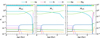 |
Fig. 6. Surface abundances of a MZAMS = 200 M⊙ star for three mass-loss rates. The blue, green, and pink shaded bars indicate the time of H, He, and C burning, respectively. |
The retained envelope of the ṀΓe model sustains the He-dominated surface and limits the exposure of the inner He shell-burning products. It becomes a WNh star around log Teff ≃ 4.5 and retains a small fraction of H on the surface during the rest of its evolution. This star ends its evolution with a He dominated surface,  , some remnant H,
  , and trace amounts of C and O,
  and
and  .
.
The ṀL/M track is the first to become a WNh at log Teff ≃ 4.7 and spends the last 15% of its MS as a WNh star. Later, during the CHeB phase, the star becomes a bare core, where He burning products are directly exposed on the stellar surface. This star loses the most mass compared to the other two models. This significant reduction also affects the core mass, enabling the star to continue igniting subsequent burning phases until core oxygen burning, before entering the PI regime and becoming dynamically unstable. The ṀL/M model ends as a WO star, with  , and
, and  , and low He abundance,
  .
.
It is worth noting that in this analysis, we do not include rotation in our tracks, as it was not the focus of the paper. Other authors, as Sabhahit et al. (2022), find that moderately rotating models (Ω/Ωcrit = 0.2) with MZAMS ≳ 200 M⊙ become chemically homogeneous during the MS, however, the evolution still remains dominated by the mass-loss. To explore this aspect, in Appendix B, we present and describe the evolution of selected VMS stellar tracks with new stellar winds and rotation. In agreement with Sabhahit et al. (2022), we find that for all MZAMS ≳ 200 M⊙, the evolution is completely dominated by the mass-loss rather than rotation, even for very rapid rotational rates (Ω/Ωcrit = 0.8).
3.3. Pre-SN and single BH masses
Figure 7 shows the pre-SN and remnant masses for all stellar tracks we computed. Pre-SN masses are shown for selected ZAMS masses in Table 4. All of the pre-SN masses of these stars are nearly the mass of the He core. As mentioned previously, lower-mass models (M ≲ 150 M⊙) evolve similarly for the different mass-loss rates used here and result in comparable pre-SN masses. In contrast, more massive stars show greater differences with increasing MZAMS. Stellar tracks computed with Ṁrdw end their evolution with masses roughly half that of their ZAMS masses, regardless of the initial mass. On the other hand, models computed with ṀΓe end with pre-SN masses ∼30−50% of their ZAMS mass, and ṀL/M models end with ∼13−40% of their initial masses. In both cases, the percentage decreases with increasing ZAMS mass. The largest pre-SN masses for the three wind recipes are 314 M⊙, 184 M⊙, and 80 M⊙ for the Ṁrdw, ṀΓe, and ṀL/M winds, respectively, all originating from the MZAMS = 600 M⊙ models.
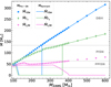 |
Fig. 7. Pre-SN mass (markers) and remnant mass (lines) as a function of the ZAMS mass for the three mass-loss rates, indicated by the marker style and color. The horizontal gray lines indicate different fates (PPISN, PISN, and DBH) based on the final He core mass. |
Pre-SN masses in M⊙ for three different wind recipes.
We use SEVN version 2.13 to compute the remnant masses based on the pre-SN properties of the stellar tracks. The models computed with the Ṁrdw rate produce a gap in the BH mass spectrum of 46 M⊙–135 M⊙, (originating from stars having initial masses ∼130 ≤ MZAMS/M⊙ ≤ 256) in general agreement with other works at LMC metallicity (Spera & Mapelli 2017; Woosley 2017; Farag et al. 2022). The BH mass gap is the same for models with ṀΓe (as we use the same prescriptions for the fate, see Sect. 2.5), but the ZAMS masses defining the gap widens, to 125 ≤ MZAMS/M⊙ ≤ 367. The ṀΓe BH masses predicted above the gap are between ∼0.3−0.4 times lighter than the BH masses of the Ṁrdw rate. The ṀL/M models do not have any upper limit to the mass gap in this mass range, as all models above 400 M⊙ die as a PISN and leave no remnant. The ṀL/M models are the only ones to produce BHs from stars with ZAMS masses of ∼140−250 M⊙. The maximum BH mass achieved with the ṀL/M wind prescription is 46 M⊙ at LMC metallicity, which is significantly lower than predictions from other studies at the same metallicity (Spera & Mapelli 2017; Giacobbo & Mapelli 2018; Farmer et al. 2019).
4. Results from the binary evolution
4.1. Wind accretion
To understand how binary evolution, particularly with stronger winds, contributes to forming VMS like those observed in R136, we first examine the process of wind accretion. This mechanism is crucial, as the stellar wind feedback onto the orbit will both produce more massive secondary stars and looser binaries, as discussed in Iorio et al. (2023), thus resulting in differences in the observed properties of the stars. Enhanced stellar winds can influence the evolution and interactions of binary systems by modifying the evolution of each star, affecting key parameters such as the maximum stellar radius (Rmax), the envelope mass (Menvelope), and the total mass (Mtotal). Moreover, stellar winds can determine whether or not a star expands during the RSG stage, thereby setting the conditions for binary interaction through mass transfer episodes. Additionally, the presence or absence of a stellar envelope will impact the likelihood of CE occurrences. Winds influence all of these processes and ultimately leave their footprint on the final mass of the stars, as discussed in Sect. 3.3.
Stellar models with enhanced wind mass-loss rates undergo different evolutionary processes in a binary system, for example, by widening the orbital separation and transferring large amounts of mass to the companion via stellar winds. For each star in the binary, we calculate the total mass accreted onto it Macc, tot, which is the cumulative mass gained from its companion from winds. We calculate the binned average of the accreted mass, expressed as a percentage of the total initial mass within the bin (of size 10 M⊙). For each ZAMS mass bin j, the percentage ⟨facc⟩j is calculated as:
 (16)
(16)
where Sj is the set of stars in the mass bin j, Macc, tot(i) is the total mass accreted by star i, and MZAMS(i) is the ZAMS mass of star i. This value represents the average fraction of mass that stars accrete relative to the total initial mass, in a given initial mass range. Figure 8 shows the ⟨facc⟩j for the primary and secondary stars for all binaries that contain at least one BH component at the end of the simulation and do not merge during stellar evolution. The total accreted material Macc, tot goes to zero if a star leaves a massless remnant (i.e., a PISN or the ejection of the companion star), which causes the percentages drop near ZAMS masses ∼170−230 M⊙ for the Ṁrdw and ṀΓe cases. The amount of mass accreted by the star, in the case of enhanced winds, can be up to ∼3% of its ZAMS mass; in one case, a star of the ṀL/M simulation accretes 39 M⊙ of material from its companion from just stellar winds alone. In comparison, the greatest amount of accreted material for the ṀΓe and Ṁrdw simulations is 24 M⊙ and 16 M⊙, respectively.
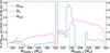 |
Fig. 8. Averaged percentage of the ZAMS mass accreted onto the primary (left) and secondary (right) per mass bin. The bins are 10 M⊙ each. The colors are the same as in Figure 7. |
The secondary star accretes more mass in general, as the primary is more massive and, therefore, loses more material, which is then available to be accreted. The simulation using ṀΓe has smaller averaged accretion around MZAMS, 2 ≃ 120 to 160 M⊙ compared to the Ṁrdw one. This is because these binaries have primaries with ZAMS masses MZAMS, 1 ≃ 120 to 345 M⊙, where most stars end evolution as PISN, thus leaving a massless remnant (see Figure 7) where the total accretion goes to zero. The Ṁrdw simulation with secondary masses of MZAMS, 2 ≃ 120 to 160 M⊙ also have primaries with MZAMS, 1 ≃ 120 to 348 M⊙, where primaries with masses MZAMS, 1 ≳ 250 M⊙ do not enter the PISN regime, and thus their accretion onto the secondary is accounted for. For the ṀL/M simulation, the absence of PISN below 350 M⊙ and the infrequency of stellar mergers allow for consistently high accretion rates in stars with ZAMS masses above 150 M⊙.
4.2. Stellar mergers
Stellar mergers represent a critical outcome of binary evolution, and have been proposed as the origin of VMS (Portegies Zwart & McMillan 2002). When two stars in a binary approach one another too closely, gravitational interactions can lead to a collision or a stellar merger. These mergers can result in a single, more massive star, exhibiting properties similar to an isolated star born with a greater ZAMS mass. The stellar radii, separation, and accretion are the main parameters determining whether the binary will merge to form a more massive star. To investigate the viability of stellar mergers being the origin of the observed VMS in R136, this section presents the characteristics of stellar mergers predicted by our simulations using different wind prescriptions, specifically focusing on whether the merged stars match the observed properties of R136a.
We search our simulations for systems with MZAMS, 1 ≥ 50 M⊙ that undergo a stellar merger and continue their evolution as a more massive star before forming a BH. When stars merge, their total mass, CO- and He-cores are summed, and the merger product inherits the phase and percentage of life of the more evolved progenitor star (for more details on the treatment of mergers and the post-merger evolution, see Iorio et al. 2023). After the collision, the interpolation algorithm in SEVN finds the new post-merger track self-consistently. We select merged objects whose luminosities and effective temperatures lie within the observational uncertainties of R136a.
The ZAMS mass distributions capable of reproducing the observed position of R136a1 on the HRD, from single stellar evolution and stellar mergers are shown in Figure 9. Our binary simulations indicate that systems merging to form more massive stars that match the position of R136a in the HRD originate from primary stars with initial masses that vary depending on the wind prescription used. For the Ṁrdw simulation, the most probable initial primary mass is 186 M⊙ in the 68% confidence interval (1σ). The ṀΓe simulations suggest a larger most probable initial primary mass of 207
 M⊙. For the ṀL/M simulations, we find a bimodal distribution around MZAMS, 1 ∼ 150 M⊙ and MZAMS, 1 ∼ 300 M⊙. This shape originates from how the single-star tracks evolve, from which stellar mergers are interpolated. The first peak comes from primaries with initial masses around ∼150 M⊙ that merge to form stars that subsequently evolve similarly to a single star born with a ZAMS mass of ∼300 M⊙. These systems are much more numerous due to the IMF used. These mergers begin the MS very near to R136a1’s location on the HRD, and spend the first ∼1 Myr within or near to the observed luminosity limits11. Similarly, the peak around 300 M⊙ arises from mergers which resemble stars born with ZAMS masses of ∼600 M⊙. While these systems are few, they directly traverse the HRD location of R136a1 twice in the later stages of the MS, and spend about ∼0.8 Myr within the luminosity limits. The stars that merge between these two regimes experience a rapid drop in luminosity, causing them to move quickly away from the location of R136a1. These mergers do not cross the observed position of the star, making these mergers the least likely to be observed. Considering the two cases, we split the results into regimes for stars with MZAMS, 1 above and below 200 M⊙. This consideration yields primary masses of 141
 M⊙ in the lower ZAMS mass regime, and 310
 M⊙ in the higher ZAMS mass regime.
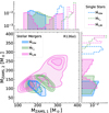 |
Fig. 9. Possible initial masses of R136a1 from single star and stellar merger origins. The shaded areas show the primary and secondary ZAMS masses of stars that merge during evolution and overlap in the HRD with the observed location of R136a1. The blue, green, and pink show results from Ṁrdw ṀΓe, and ṀL/M, respectively. The dashed histograms show the initial mass from single stellar evolution. |
The single star models reproducing the observed HRD position of R136a1 suggest initial single star masses over 100 M⊙ larger than from binary evolution: the Ṁrdw and ṀΓe tracks give MZAMS = 315 M⊙ and MZAMS = 389
 M⊙, respectively. The single star result from the ṀL/M tracks give 359
 M⊙ as the most probable initial mass within 1σ. These results highlight a key implication for the initial mass required to form a very massive object like R136a1: if the observed VMS was formed from a binary stellar merger, lower initial masses, and possibly a lower upper limit on the IMF, are needed to explain the star’s formation, compared to the evolution scenario of a single star.
For stellar merger products of systems that match the location of R136a1 in the HRD, the post-merger masses within 1σ are 278 M⊙ for the Ṁrdw simulation, 200
 M⊙ for the ṀΓe simulation, and 191
 M⊙ in the ṀL/M simulation. Single stellar evolution models predict comparable current mass for stars that occupy the same HRD location, listed in Table 3. This significant overlap in predicted current masses implies that the current mass of R136a1 is not a strong diagnostic for discriminating between an origin of a single star or a stellar merger product. We provide and discuss the possible initial and current masses for R136a2 and R136a3 in Appendix A.
Stellar mergers occur while the primary is on the MS 83% of the time for the Ṁrdw simulations, and 82% for both the ṀΓe and ṀL/M simulations. The Ṁrdw simulation is also more likely to merge during CHeB than the other simulations, as stars with Ṁrdw winds expand more during this phase. On the other hand, the simulations with stronger winds have more stellar mergers during H and He-shell burning phases than the Ṁrdw simulation.
The most common stellar merger pathway for all three wind recipes is by beginning a stable RLOF that circularizes the orbit, and ends in the merger of the two stars. A RLOF occurs when the radius of a star becomes equivalent to or larger than the RL radius and transfers mass until it leads to a merger or a CE configuration. The RLOF pathway leading directly to a stellar merger occurs in 66% of all stellar mergers, regardless of the wind recipe, while the RLOF pathway leading to a CE phase and then a merger occurs in 3.9% of all stellar mergers.
4.3. Remnant mass spectrum
The masses and formation channels of BHs are linked to the evolution of the progenitor star; therefore, the properties of predicted BH populations serve as an indirect test of the stellar and binary evolution models. BH populations arising as a result of stellar mergers and from nonmerging binary BHs (BBHs) are shown in Figure 10. For stars with ZAMS masses below 100 M⊙, we use the same stellar tracks employing standard wind recipes for all three simulations. Therefore, the BH populations have similar distributions for lower ZAMS masses and are not shown in the figure for clarity. From our simulations, we find that the distribution of single BHs formed via stellar mergers changes considerably depending on the stellar winds assumed. Simulations with enhanced wind mass loss form fewer massive BHs, particularly with remnant masses above 100 M⊙. As mentioned in Sect. 3.1, these stars expand less during evolution due to substantial mass-loss, making them less likely to fill their Roche Lobe. The enhanced mass-loss also widens the orbit, allowing the stars to evolve with fewer binary interactions or stellar mergers than in the standard wind case. The extreme winds of the ṀL/M simulation erode the stellar mass so much that even the VMSs that merge during evolution cannot form a BH above ∼50 M⊙. This is a stark contrast with the Ṁrdw and ṀΓe simulations, which generally form more massive BHs (MBH > 100 M⊙) after a stellar merger when compared to the resulting BH mass from single stellar evolution.
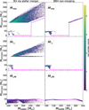 |
Fig. 10. Black hole number counts for BHs formed from stellar mergers (left) and nonmerging BBHs (right) for the simulations with Ṁrdw (top), ṀΓe (middle), and ṀL/M (bottom). The dashed pink lines indicate BH masses from single stellar evolution. |
The populations of binary BHs that do not merge within a Hubble time are shown in the right panel of Figure 10. The Ṁrdw is the only one that can form nonmerging BHs above the PI mass gap. These BHs arise from binaries that experience stable mass transfer before the first BH formation. There is a lack of nonmerging binary BHs from the ṀΓe simulation with ZAMS masses ≳140 M⊙, due to the stars experiencing PISN. Finally, the ṀL/M simulation forms nonmerging BHs with masses near the result for single stellar evolution, as they too arise from binaries experiencing episodes of stable mass transfer.
Finally, the BBHs that do merge within a Hubble time originate primarily from ‘lower-mass’ progenitors (less than ∼80 M⊙), so the differences between wind prescriptions are subtle. To highlight the differences in the component masses of these mergers, Figure 11 shows the primary (MBH, 1) and secondary (MBH, 2) BH masses of BBHs that merge within a Hubble time. The most common primary BH masses lie between 3 and 9 M⊙ for all mass-loss rates. These BHs originate from the more numerous lower-mass stars with ZAMS masses in the range of 20−40 M⊙, which are not the focus of this study, and the contour plot shows only BHs with masses > 20 M⊙. More striking differences appear in the high-mass tail of the distributions: the ṀΓe and ṀL/M simulations yield many more massive primaries (MBH, 1 ≥ 30 M⊙), with a peak around ∼35 M⊙ for ṀΓe and at ∼45 M⊙ for ṀL/M. These systems also produce a peak in the secondary masses around MBH, 2 ≃ 40 M⊙. This is noteworthy because it suggests the emergence of such peaks in the high-mass side is not only due to prescriptions employed for the final fate and the binary stellar evolution processes (e.g., van Son et al. 2022; Briel et al. 2023; Farrah et al. 2023; Golomb et al. 2024; Hendriks et al. 2023; Dorozsmai & Toonen 2024; Ugolini et al., in prep.); rather, they result purely from imposing different stellar wind prescriptions in the stellar tracks. The binaries with standard winds tend to expand, increasing their likelihood of interacting and merging during evolution, precluding them from a BBH configuration. Conversely, the models with stronger winds remain more compact and are less likely to merge as stars, thus allowing for the survival of binaries with larger initial masses that can then form massive merging BHs. We find that simulations with enhanced winds tend to have primary and secondary components with similar masses, at variance with standard wind simulations, which exhibit a broader distribution of component mass ratios. Additionally, the LIGO-Virgo-Kagra (LVK) collaboration has detected gravitational-wave emission from BBH mergers with secondary BH masses ≳40 M⊙ (Abbott et al. 2020, 2023, 2024), a mass range only reproduced with our ṀΓe and ṀL/M simulations. Therefore, to form such massive BHs maintaining this metallicity using the Ṁrdw winds, other formation scenarios are needed, such as dynamical interaction in a cluster and/or hierarchical BH mergers. Features of the merging BBHs, such as masses, formation channels, and binary properties, are discussed in further detail in Appendix C.
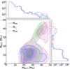 |
Fig. 11. Primary vs. secondary BH masses for BBHs that merge in a Hubble time. The contour plot shows the mergers for binaries with MBH, 1 ≥ 20 M⊙, while the distributions show the full mass range of primary and secondary BH masses on the top and right. The solid blue, dashed green, and dash-dotted pink lines refer to simulations with stellar tracks computed with the Ṁrdw, ṀΓe, and ṀL/M rates, respectively. |
Figure 12 shows the BH mass histograms of different BH populations computed with tracks using different stellar winds. In all three simulations, the single BHs (formed from either ejecting or merging with the companion) can partially fill the BH mass gap from single stars, forming BHs with masses up to ∼90 M⊙. These BHs account for 59%, 58%, and 57% of all BHs formed from the Ṁrdw, ṀΓe, and ṀL/M simulations. The binary BHs that do not merge in a Hubble time have a maximum BH mass of 198 M⊙ for the Ṁrdw case, while for the ṀΓe and ṀL/M cases it is 50 M⊙. The nonmerging BBHs account for 35.7% (Ṁrdw), 36.4% (ṀΓe), and 37.8% (ṀL/M) of BHs formed from the simulations. Interestingly, the ṀΓe and ṀL/M simulations can fill part of the BH mass gap from single stars with their merged BH masses, up to ∼90 M⊙. This is in contrast with the Ṁrdw simulation, in which the most massive BH from the merger of a BBH within a Hubble time is 64 M⊙. These BH mergers account for 5.7%, 5.9%, and 5.2% of BHs formed in the Ṁrdw, ṀΓe, and ṀL/M simulations.
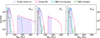 |
Fig. 12. Number counts of BHs from the simulations with Ṁrdw (left), ṀΓe (center), and ṀL/M (right). The shaded purple shows the result from single stellar evolution. The dashed pink, solid blue, and dash-dotted green lines show results from binary evolution of single BHs, binary BHs that do not merge within a Hubble time, and the resulting BH mass of a BBH merger that merged within a Hubble time, respectively. |
5. Discussion
While our simulations offer interesting insights into the evolution of massive stars with updated stellar winds and their implications for the formation of VMS and remnant populations, it is necessary to acknowledge a few uncertainties and limitations in the modeling. Here, we outline a few key caveats that should be considered in this work.
A specific source of uncertainty in single stellar evolution lies in the validity of the new mass-loss prescriptions in the post-MS phases. Stars spend most of their lives on the MS and indeed lose the most mass via stellar winds during this stage, and therefore, the post-MS mass-loss rates affect the final mass of the star far less than MS mass loss, in the VMS regime.
Rotation is another fundamental physical process that is intricately involved in stellar evolution and mass-loss, and remains challenging to model comprehensively in population synthesis studies. Stellar rotation can increase the mixing of chemical elements, altering the nuclear burning lifetimes and abundance composition at the surface (Maeder 2009). We ran models with rotation (see Appendix B), and found that the evolution is more strongly affected by the mass-loss from stellar winds than rotational mixing for moderate rotational rates (Ω/Ωcrit ≲ 0.6). This is because VMSs have large convective cores during the MS, and moderate rotation has a negligible effect on VMS evolution (Yusof et al. 2013). In addition, Bestenlehner et al. (2014) found rotational mixing plays a relatively unimportant role in luminous massive stars with very strong mass-loss, instead, the mass-loss rate has a strong correlation with the surface He enrichment due to winds stripping the outer layers.
Uncertainties in the final fate of VMS propagate into uncertainties in the remnant properties. Of these, the edges of the PI mass gap pose as a source of uncertainty in our predictions. The conditions that give rise to pair creation depend on the CO core mass and its composition (C/O), which are affected by evolutionary processes such as mass-loss, convection, overshooting, and nuclear reactions. Many studies have shown how the edges of the PI mass gap change when altering major sources of uncertainty, such as variations in the 12C(α, γ)16O reaction rates (Farmer et al. 2019, 2020), dredge-up episodes (Costa et al. 2021), pulsation-driven mass-loss (Volpato et al. 2023) with rotation (Volpato et al. 2024), and other uncertainties in massive star evolution (Woosley & Heger 2021; Vink et al. 2021). Additionally, the prescriptions adopted to compute the final remnant mass are also subject to uncertainty.
Binary evolution modeling propagates the uncertainties found in single-star models, and adds additional sources and challenges. The main ones are described in Iorio et al. (2023). The CE phase is one of the most uncertain processes in binary stellar evolution, due to the hefty computational challenges (Ivanova et al. 2013, 2020; MacLeod et al. 2017; Fragos et al. 2019). As a result, hydrodynamical simulations face challenges in modeling the full CE evolution: simulations may omit key physical processes, including recombination energy, nuclear reactions in accreted material, neutrino cooling, and energy transport mechanisms (Röpke & De Marco 2023). Moreover, the definition of binding energy and the core mass definition used can alter the resulting binding energy of the star, affecting binary interactions and the merger rate density (Sgalletta et al., in prep.). The mass transfer stability conditions are also uncertain, and can heavily influence the merger rate densities (Olejak et al. 2021; Dorozsmai & Toonen 2024). Finally, due to the scale of these simulations and the necessary computational efficiency, the precise tracking of surface abundances from stellar mergers is not accurately modeled. Therefore, we cannot provide constraints on the surface chemical compositions of the post-merger products discussed in Section 4.2. Hydrodynamical simulations following the evolution of a post-collision star suggested, however, that the stellar surface would have a higher helium content (Costa et al. 2022). Future works will be dedicated to the hydrodynamic modeling of stellar mergers to trace the surface composition in detail.
Finally, we cannot make conclusive comparisons with the LVK data by using the newly implemented prescriptions for stellar winds, as our focus on VMSs in the LMC at a single metallicity of Z = 0.006. Future studies will examine the impact of these new prescriptions on the evolution of single and binary stars across different metallicities.
6. Conclusion
We have presented new stellar evolution tracks that were computed with enhanced stellar wind mass-loss rates for VMSs. We ran single stellar models with 100 ≤ MZAMS/M⊙ ≤ 600 at the LMC metallicity (Z = 0.006) for the three mass-loss rates we discussed, based on theoretical and observational studies that suggested that the dependence on the Eddington parameter increases when VMSs approach the Eddington limit.
We presented the possible evolution of a population of massive binaries by employing our new stellar models in the SEVN binary population synthesis code. We investigated stellar mergers as a possible origin of observed VMSs, such as those in R136a, and compared the implications with the results from single stellar evolution. We characterized the different BH populations and formation channels that arise from altering the wind prescription. We summarize our main results below.
-
The stellar tracks computed with the new winds, ṀΓe and Ṁrdw, inflate less on the MS. They remain hotter and more compact as a result of the enhanced mass loss than in models that are computed with the standard rates, Ṁrdw. The tracks with stronger winds spend more time within the observed narrow Teff range of observed VMSs in R136a, and they reproduce their observed properties better.
-
Using the statistical tool PARAM, we found that only stellar tracks that are computed with the ṀΓe wind prescription can fit the observed features of R136a with stellar age estimates of ∼1.3−1.6 Myr. This age determination agrees with age estimates from other studies.
-
The amount of the mass that is retained by stars at the pre-SN stage varies notably with the adopted wind prescription. With the Ṁrdw winds, stars typically retain 48% to 52% of their ZAMS mass. In contrast, the ṀΓe and ṀL/M models result in appreciably higher mass loss, and the percentage of the retained mass depends on the ZAMS mass. For ṀΓe, the retained mass ranges from 30% to 52%, and it decreases as the ZAMS mass increases. The ṀL/M winds predict the most extreme mass loss, resulting in stars that only retain 13% to 42% of their ZAMS mass at the pre-SN stage, and it also decreases with increasing initial mass.
-
We investigated the possible origins of the VMS R136a1 from single and binary evolution. If binary stellar mergers are the origin of R136a1, then our models suggest a primary initial upper mass limit of 186 M⊙ (for the Ṁrdw case), 207 M⊙ (for the ṀΓe case), and 141 and 310 M⊙ (for the ṀL/M classes 1 and 2). Conversely, when the origin of this VMS is explained through single stellar evolution, a higher upper initial mass limit from 315 M⊙ (for the Ṁrdw case) to 390 M⊙ (for the enhanced winds) is required. In either case, we established a strict upper limit on the ZAMS mass for R136a1, which must be ≲400 M⊙, regardless of the wind prescription.
-
From the simulation of binary populations with different winds, we found unique BH distributions for each wind recipe. Simulations with enhanced winds are less likely to merge during the stellar evolution because the inflation is suppressed on the MS. As a consequence, these systems have fewer stellar mergers and produce fewer intermediate-mass BHs (with masses above the PISN gap) than standard stellar winds.
-
For binary BHs that merge within a Hubble time, only the ṀΓe and ṀL/M simulations were able to have secondaries with masses > 32 M⊙, in agreement with observed BBH mergers. Moreover, these two simulations produced many more primaries with BH masses > 30 M⊙ than the Ṁrdw simulation.
We consider the star has reached the TAMS when the central H abundance reaches  in mass fraction.
See Appendix B for rotating tracks.
Approximated value from [M/H] = log((Z/X)/0.0207) (Bressan et al. 2012).
Penetrative overshooting is described in Bressan et al. (1981).
See Fig. 3 of Smith (2014) for an overview including other mass-loss prescriptions at solar Z.
CHeB starts after the TAMS when 1% of the central helium has been burnt, and lasts until it reaches  ≤ 10−6.
The limits discussed here refer only to the luminosity and effective temperature (and their 1σ uncertainty) of R136a1.
Acknowledgments
The authors thank Iorio, G., for the helpful discussions. We acknowledge the Italian Ministerial grant PRIN2022, “Radiative opacities for astrophysical applications”, no. 2022NEXMP8. GC acknowledges partial financial support from European Union–Next Generation EU, Mission 4, Component 2, CUP: C93C24004920006, project ‘FIRES’. MS, CU, and CS acknowledge their participation in the 2024 Unconventional Thinking Tank Conference, supported by INAF, during which part of this work was developed. MS acknowledges financial support from Large Grant INAF 2024 “Envisioning Tomorrow: prospects and challenges for multimessenger astronomy in the era of Rubin and Einstein Telescope”, from Fondazione ICSC, Spoke 3 Astrophysics and Cosmos Observations, National Recovery and Resilience Plan (Piano Nazionale di Ripresa e Resilienza, PNRR) Project ID CN_00000013 “Italian Research Center on High-Performance Computing, Big Data and Quantum Computing” funded by MUR Missione 4 Componente 2 Investimento 1.4: Potenziamento strutture di ricerca e creazione di “campioni nazionali di R&S (M4C2-19)” – Next Generation EU (NGEU), and from the program “Data Science methods for Multi-Messenger Astrophysics & Multi-Survey Cosmology” funded by the Italian Ministry of University and Research, Programmazione triennale 2021/2023 (DM n.2503 dd. 09/12/2019), Programma Congiunto Scuole.
References
- Abbott, B. P., Abbott, R., Abbott, T. D., et al. 2016, Phys. Rev. Lett., 116, 061102 [Google Scholar]
- Abbott, R., Abbott, T. D., Abraham, S., et al. 2020, Phys. Rev. Lett., 125, 101102 [Google Scholar]
- Abbott, R., Abbott, T. D., Acernese, F., et al. 2023, Phys. Rev. X, 13, 041039 [Google Scholar]
- Abbott, R., Abbott, T. D., Acernese, F., et al. 2024, Phys. Rev. D, 109, 022001 [NASA ADS] [CrossRef] [Google Scholar]
- Bestenlehner, J. M. 2020, MNRAS, 493, 3938 [Google Scholar]
- Bestenlehner, J. M., Gräfener, G., Vink, J. S., et al. 2014, A&A, 570, A38 [NASA ADS] [CrossRef] [EDP Sciences] [Google Scholar]
- Bestenlehner, J. M., Crowther, P. A., Caballero-Nieves, S. M., et al. 2020, MNRAS, 499, 1918 [Google Scholar]
- Björklund, R., Sundqvist, J. O., Singh, S. M., Puls, J., & Najarro, F. 2023, A&A, 676, A109 [NASA ADS] [CrossRef] [EDP Sciences] [Google Scholar]
- Böhm-Vitense, E. 1958, Z. Astrophys., 46, 108 [Google Scholar]
- Brands, S. A., de Koter, A., Bestenlehner, J. M., et al. 2022, A&A, 663, A36 [Google Scholar]
- Bressan, A. G., Chiosi, C., & Bertelli, G. 1981, A&A, 102, 25 [Google Scholar]
- Bressan, A., Marigo, P., Girardi, L., et al. 2012, MNRAS, 427, 127 [NASA ADS] [CrossRef] [Google Scholar]
- Briel, M. M., Stevance, H. F., & Eldridge, J. J. 2023, MNRAS, 520, 5724 [Google Scholar]
- Broekgaarden, F. S., Stevenson, S., & Thrane, E. 2022, ApJ, 938, 45 [CrossRef] [Google Scholar]
- Brott, I., de Mink, S. E., Cantiello, M., et al. 2011, A&A, 530, A115 [NASA ADS] [CrossRef] [EDP Sciences] [Google Scholar]
- Caffau, E., Ludwig, H. G., Steffen, M., Freytag, B., & Bonifacio, P. 2011, Sol. Phys., 268, 255 [Google Scholar]
- Cassinelli, J. P., Mathis, J. S., & Savage, B. D. 1981, Science, 212, 1497 [NASA ADS] [CrossRef] [Google Scholar]
- Castor, J. I., Abbott, D. C., & Klein, R. I. 1975, ApJ, 195, 157 [Google Scholar]
- Chen, Y., Bressan, A., Girardi, L., et al. 2015, MNRAS, 452, 1068 [Google Scholar]
- Choudhury, S., Subramaniam, A., & Cole, A. A. 2016, MNRAS, 455, 1855 [NASA ADS] [CrossRef] [Google Scholar]
- Choudhury, S., de Grijs, R., Bekki, K., et al. 2021, MNRAS, 507, 4752 [CrossRef] [Google Scholar]
- Costa, G., Girardi, L., Bressan, A., et al. 2019a, A&A, 631, A128 [NASA ADS] [CrossRef] [EDP Sciences] [Google Scholar]
- Costa, G., Girardi, L., Bressan, A., et al. 2019b, MNRAS, 485, 4641 [NASA ADS] [CrossRef] [Google Scholar]
- Costa, G., Bressan, A., Mapelli, M., et al. 2021, MNRAS, 501, 4514 [NASA ADS] [CrossRef] [Google Scholar]
- Costa, G., Ballone, A., Mapelli, M., & Bressan, A. 2022, MNRAS, 516, 1072 [NASA ADS] [CrossRef] [Google Scholar]
- Costa, G., Shepherd, K. G., Bressan, A., et al. 2025, A&A, 694, A193 [NASA ADS] [CrossRef] [EDP Sciences] [Google Scholar]
- Crowther, P. A., Schnurr, O., Hirschi, R., et al. 2010, MNRAS, 408, 731 [Google Scholar]
- Crowther, P. A., Caballero-Nieves, S. M., Bostroem, K. A., et al. 2016, MNRAS, 458, 624 [Google Scholar]
- da Silva, L., Girardi, L., Pasquini, L., et al. 2006, A&A, 458, 609 [NASA ADS] [CrossRef] [EDP Sciences] [Google Scholar]
- de Jager, C., Nieuwenhuijden, H., & van der Hucht, K. A. 1988, Bulletin d’Information du Centre de Donnees Stellaires, 35, 141 [Google Scholar]
- de Koter, A., Heap, S. R., & Hubeny, I. 1998, ApJ, 509, 879 [Google Scholar]
- Dorozsmai, A., & Toonen, S. 2024, MNRAS, 530, 3706 [NASA ADS] [CrossRef] [Google Scholar]
- Eggenberger, P., Meynet, G., Maeder, A., et al. 2008, Ap&SS, 316, 43 [Google Scholar]
- Evans, C. J., Taylor, W. D., Hénault-Brunet, V., et al. 2011, A&A, 530, A108 [NASA ADS] [CrossRef] [EDP Sciences] [Google Scholar]
- Farag, E., Renzo, M., Farmer, R., Chidester, M. T., & Timmes, F. X. 2022, ApJ, 937, 112 [NASA ADS] [CrossRef] [Google Scholar]
- Farmer, R., Renzo, M., de Mink, S. E., Marchant, P., & Justham, S. 2019, ApJ, 887, 53 [Google Scholar]
- Farmer, R., Renzo, M., de Mink, S. E., Fishbach, M., & Justham, S. 2020, ApJ, 902, L36 [CrossRef] [Google Scholar]
- Farrah, D., Petty, S., Croker, K. S., et al. 2023, ApJ, 943, 133 [NASA ADS] [CrossRef] [Google Scholar]
- Fragos, T., Andrews, J. J., Ramirez-Ruiz, E., et al. 2019, ApJ, 883, L45 [Google Scholar]
- Freitag, M., Gürkan, M. A., & Rasio, F. A. 2006, MNRAS, 368, 141 [NASA ADS] [Google Scholar]
- Fryer, C. L., Belczynski, K., Wiktorowicz, G., et al. 2012, ApJ, 749, 91 [Google Scholar]
- Fu, X., Bressan, A., Marigo, P., et al. 2018, MNRAS, 476, 496 [NASA ADS] [CrossRef] [Google Scholar]
- Gallagher, J. S. 1989, Astrophys. Space Sci. Lib., 157, 185 [Google Scholar]
- Georgy, C., Ekström, S., Eggenberger, P., et al. 2013, A&A, 558, A103 [NASA ADS] [CrossRef] [EDP Sciences] [Google Scholar]
- Giacobbo, N., & Mapelli, M. 2018, MNRAS, 480, 2011 [Google Scholar]
- Golomb, J., Isi, M., & Farr, W. 2024, ApJ, 976, 121 [NASA ADS] [CrossRef] [Google Scholar]
- Gormaz-Matamala, A. C., Cuadra, J., Ekström, S., et al. 2024, A&A, 687, A290 [NASA ADS] [CrossRef] [EDP Sciences] [Google Scholar]
- Gräfener, G., & Hamann, W. R. 2008, A&A, 482, 945 [Google Scholar]
- Gräfener, G., Vink, J. S., de Koter, A., & Langer, N. 2011, A&A, 535, A56 [NASA ADS] [CrossRef] [EDP Sciences] [Google Scholar]
- Heger, A., & Woosley, S. E. 2002, ApJ, 567, 532 [Google Scholar]
- Heger, A., Langer, N., & Woosley, S. E. 2000, ApJ, 528, 368 [NASA ADS] [CrossRef] [Google Scholar]
- Hendriks, D. D., van Son, L. A. C., Renzo, M., Izzard, R. G., & Farmer, R. 2023, MNRAS, 526, 4130 [NASA ADS] [CrossRef] [Google Scholar]
- Humphreys, R. M., & Davidson, K. 1979, ApJ, 232, 409 [Google Scholar]
- Hurley, J. R., Tout, C. A., & Pols, O. R. 2002, MNRAS, 329, 897 [Google Scholar]
- Iorio, G., Mapelli, M., Costa, G., et al. 2023, MNRAS, 524, 426 [NASA ADS] [CrossRef] [Google Scholar]
- Ivanova, N., Justham, S., Chen, X., et al. 2013, A&ARv, 21, 59 [Google Scholar]
- Ivanova, N., Justham, S., & Ricker, P. 2020, Common Envelope Evolution (IOP Publishing) [Google Scholar]
- Josiek, J., Ekström, S., & Sander, A. A. C. 2024, A&A, 688, A71 [NASA ADS] [CrossRef] [EDP Sciences] [Google Scholar]
- Josiek, J., Sander, A. A. C., & Bernini-Peron, M. 2025, A&A, 697, A193 [NASA ADS] [CrossRef] [EDP Sciences] [Google Scholar]
- Justham, S., Podsiadlowski, P., & Vink, J. S. 2014, ApJ, 796, 121 [NASA ADS] [CrossRef] [Google Scholar]
- Kobulnicky, H. A., & Fryer, C. L. 2007, ApJ, 670, 747 [NASA ADS] [CrossRef] [Google Scholar]
- Köhler, K., Langer, N., de Koter, A., et al. 2015, A&A, 573, A71 [NASA ADS] [CrossRef] [EDP Sciences] [Google Scholar]
- Kroupa, P. 2001, MNRAS, 322, 231 [NASA ADS] [CrossRef] [Google Scholar]
- Lattanzi, M. G., Hershey, J. L., Burg, R., et al. 1994, ApJ, 427, L21 [CrossRef] [Google Scholar]
- MacLeod, M., Antoni, A., Murguia-Berthier, A., Macias, P., & Ramirez-Ruiz, E. 2017, ApJ, 838, 56 [Google Scholar]
- Maeder, A. 2009, Physics, Formation and Evolution of Rotating Stars (Berlin, Heidelberg: Springer) [Google Scholar]
- Mapelli, M., Spera, M., Montanari, E., et al. 2020, ApJ, 888, 76 [NASA ADS] [CrossRef] [Google Scholar]
- Marchant, P., Renzo, M., Farmer, R., et al. 2019, ApJ, 882, 36 [Google Scholar]
- Martinet, S., Meynet, G., Ekström, S., Georgy, C., & Hirschi, R. 2023, A&A, 679, A137 [NASA ADS] [CrossRef] [EDP Sciences] [Google Scholar]
- Martins, F., Hillier, D. J., Paumard, T., et al. 2008, A&A, 478, 219 [NASA ADS] [CrossRef] [EDP Sciences] [Google Scholar]
- Mason, B. D., Hartkopf, W. I., Gies, D. R., Henry, T. J., & Helsel, J. W. 2009, AJ, 137, 3358 [Google Scholar]
- Massey, P., & Hunter, D. A. 1998, ApJ, 493, 180 [NASA ADS] [CrossRef] [Google Scholar]
- McEvoy, C. M., Dufton, P. L., Evans, C. J., et al. 2015, A&A, 575, A70 [NASA ADS] [CrossRef] [EDP Sciences] [Google Scholar]
- Menon, A., & Heger, A. 2017, MNRAS, 469, 4649 [NASA ADS] [Google Scholar]
- Nguyen, C. T., Costa, G., Girardi, L., et al. 2022, A&A, 665, A126 [NASA ADS] [CrossRef] [EDP Sciences] [Google Scholar]
- Nugis, T., & Lamers, H. J. G. L. M. 2000, A&A, 360, 227 [NASA ADS] [Google Scholar]
- Olejak, A., Belczynski, K., & Ivanova, N. 2021, A&A, 651, A100 [NASA ADS] [CrossRef] [EDP Sciences] [Google Scholar]
- Petrovic, J., Langer, N., & van der Hucht, K. A. 2005, A&A, 435, 1013 [NASA ADS] [CrossRef] [EDP Sciences] [Google Scholar]
- Podsiadlowski, P., Joss, P. C., & Rappaport, S. 1990, A&A, 227, L9 [NASA ADS] [Google Scholar]
- Portegies Zwart, S. F., & McMillan, S. L. W. 2002, ApJ, 576, 899 [Google Scholar]
- Ramírez-Agudelo, O. H., Sana, H., de Koter, A., et al. 2017, A&A, 600, A81 [NASA ADS] [CrossRef] [EDP Sciences] [Google Scholar]
- Rodrigues, T. S., Girardi, L., Miglio, A., et al. 2014, MNRAS, 445, 2758 [Google Scholar]
- Rodrigues, T. S., Bossini, D., Miglio, A., et al. 2017, MNRAS, 467, 1433 [NASA ADS] [Google Scholar]
- Röpke, F. K., & De Marco, O. 2023, Liv. Rev. Comput. Astrophys., 9, 2 [CrossRef] [Google Scholar]
- Sabhahit, G. N., & Vink, J. S. 2025, A&A, 693, A10 [NASA ADS] [CrossRef] [EDP Sciences] [Google Scholar]
- Sabhahit, G. N., Vink, J. S., Higgins, E. R., & Sander, A. A. C. 2022, MNRAS, 514, 3736 [NASA ADS] [CrossRef] [Google Scholar]
- Sabín-Sanjulián, C., Simón-Díaz, S., Herrero, A., et al. 2014, A&A, 564, A39 [NASA ADS] [CrossRef] [EDP Sciences] [Google Scholar]
- Sabín-Sanjulián, C., Simón-Díaz, S., Herrero, A., et al. 2017, A&A, 601, A79 [NASA ADS] [CrossRef] [EDP Sciences] [Google Scholar]
- Sana, H., de Mink, S. E., de Koter, A., et al. 2012, Science, 337, 444 [Google Scholar]
- Sana, H., de Mink, S. E., de Koter, A., et al. 2013, ASP Conf. Ser., 470, 141 [Google Scholar]
- Sander, A., Hainich, R., Hamann, W. R., et al. 2019, Anchoring Mass-loss and Metallicity for the WR Population in M31 – A Prototype Study, HST Proposal. Cycle 27, 15822 [Google Scholar]
- Savage, B. D., Fitzpatrick, E. L., Cassinelli, J. P., & Ebbets, D. C. 1983, ApJ, 273, 597 [NASA ADS] [CrossRef] [Google Scholar]
- Schneider, F. R. N., Langer, N., de Koter, A., et al. 2014, A&A, 570, 66 [Google Scholar]
- Schneider, F. R. N., Sana, H., Evans, C. J., et al. 2018, Science, 359, 69 [NASA ADS] [CrossRef] [Google Scholar]
- Schwarzschild, M. 1958, Structure and Evolution of the Stars (Princeton: Princeton University Press) [Google Scholar]
- Shenar, T., Sana, H., Crowther, P. A., et al. 2023, A&A, 679, A36 [NASA ADS] [CrossRef] [EDP Sciences] [Google Scholar]
- Smith, N. 2014, ARA&A, 52, 487 [NASA ADS] [CrossRef] [Google Scholar]
- Smith, N., & Conti, P. S. 2008, ApJ, 679, 1467 [NASA ADS] [CrossRef] [Google Scholar]
- Smith, N., & Tombleson, R. 2015, MNRAS, 447, 598 [NASA ADS] [CrossRef] [Google Scholar]
- Spera, M., & Mapelli, M. 2017, MNRAS, 470, 4739 [Google Scholar]
- Spera, M., Mapelli, M., & Bressan, A. 2015, MNRAS, 451, 4086 [NASA ADS] [CrossRef] [Google Scholar]
- Spera, M., Mapelli, M., Giacobbo, N., et al. 2019, MNRAS, 485, 889 [Google Scholar]
- Spera, M., Trani, A. A., & Mencagli, M. 2022, Galaxies, 10, 76 [NASA ADS] [CrossRef] [Google Scholar]
- Stothers, R. B. 1999, MNRAS, 305, 365 [NASA ADS] [CrossRef] [Google Scholar]
- van Son, L. A. C., de Mink, S. E., Renzo, M., et al. 2022, ApJ, 940, 184 [NASA ADS] [CrossRef] [Google Scholar]
- Vanbeveren, D., & Conti, P. S. 1980, A&A, 88, 230 [NASA ADS] [Google Scholar]
- Vink, J. S. 2015, in Wolf-Rayet Stars, eds. W. R. Hamann, A. Sander, & H. Todt, 133 [Google Scholar]
- Vink, J. S., & Gräfener, G. 2012, ApJ, 751, L34 [Google Scholar]
- Vink, J. S., de Koter, A., & Lamers, H. J. G. L. M. 2000, A&A, 362, 295 [Google Scholar]
- Vink, J. S., de Koter, A., & Lamers, H. J. G. L. M. 2001, A&A, 369, 574 [NASA ADS] [CrossRef] [EDP Sciences] [Google Scholar]
- Vink, J. S., Muijres, L. E., Anthonisse, B., et al. 2011, A&A, 531, A132 [NASA ADS] [CrossRef] [EDP Sciences] [Google Scholar]
- Vink, J. S., Higgins, E. R., Sander, A. A. C., & Sabhahit, G. N. 2021, MNRAS, 504, 146 [NASA ADS] [CrossRef] [Google Scholar]
- Volpato, G., Marigo, P., Costa, G., et al. 2023, ApJ, 944, 40 [NASA ADS] [CrossRef] [Google Scholar]
- Volpato, G., Marigo, P., Costa, G., et al. 2024, ApJ, 961, 89 [NASA ADS] [CrossRef] [Google Scholar]
- Weigelt, G., & Baier, G. 1985, A&A, 150, L18 [NASA ADS] [Google Scholar]
- Woosley, S. E. 2017, ApJ, 836, 244 [Google Scholar]
- Woosley, S. E., & Heger, A. 2021, ApJ, 912, L31 [NASA ADS] [CrossRef] [Google Scholar]
- Yusof, N., Hirschi, R., Meynet, G., et al. 2013, MNRAS, 433, 1114 [NASA ADS] [CrossRef] [Google Scholar]
Appendix A: Mass estimates for R136a2 and R136a3
Here we briefly discuss the possible origins of the VMSs R136a2 and R136a3. The initial and current mass derived from single and binary mergers that match the observed properties of the R136 stars are listed in Table A.1, including mass estimates from literature. Figure A.1 shows the initial mass distributions for R136a2 from single and binary stellar merger origins. Similarly to our results of R136a1, a single star origin necessitates a ZAMS mass ∼ 100 M⊙ larger than the ZAMS masses from stellar merger origin. The estimates from a single star origin, both from literature and from all of our wind recipes, generally suggest ZAMS masses > 200 M⊙. Even so, the current mass derived is generally in agreement between single and binary origins, for models using the same wind prescription.
Mass estimates of R136a from single and binary stellar mergers for the winds described in this work.
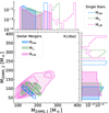 |
Fig. A.1. The possible initial masses of R136a2 from single star and stellar merger origins. The shaded areas show the primary and secondary ZAMS masses of stars that merge during evolution and overlap in the HRD with the observed location of R136a2. The blue, green, and pink show results from Ṁrdw ṀΓe, and ṀL/M, respectively. The dashed histograms show the initial mass from single stellar evolution. |
Finally, the 1σ mass estimates from single and binary origins are shown in Figure A.2 for the best fit to the R136a3 star. As expected, the stellar merger origin necessitates a primary ZAMS mass ∼100 M⊙ less than needed for a single star origin. We provide two classes of solutions for the best fit ZAMS masses of ṀL/M, for primaries with masses above and below 200 M⊙, as was done for R136a1. Interestingly, both stellar mergers and single star current mass estimates from ṀΓe and ṀL/M agree within the uncertainty of other mass estimates from literature. In contrast, those using Ṁrdw are much larger than other estimates. This is because the Ṁrdw tracks fit the stars better earlier in the evolution (see Table 3), when they have not lost significant amounts of mass yet. The Ṁrdw binaries are more likely to merge earlier in evolution compared to the enhanced wind simulations, and therefore also retain more of their initial mass than the enhanced wind simulations.
Appendix B: Rotating tracks
Stellar rotation is a crucial aspect that influences the evolution of massive stars; for example, it increases the mixing of chemical elements, altering the nuclear burning lifetimes and surface abundance composition (Maeder 2009). As such, rotation can also play a critical role in determining the final fate of the star.
We compute full stellar evolution models for stars with masses 100 ≤ MZAMS/M⊙ ≤ 350. The rotation processes are described in Costa et al. (2019a,b), Nguyen et al. (2022). Models are computed with initial rotation rates ω = 0.4, ω = 0.6, and 100 ≤ MZAMS/M⊙ ≤ 200 for ω = 0.8. ω is the fraction of the initial angular velocity to the critical angular velocity, that is, ω = Ωini/Ωcrit. Our models account for the mass-loss enhancement due to rotation, following the prescriptions from Heger et al. (2000), which include a dependency on the ratio between the surface velocity and the break-up velocity. We take into account mechanical mass-loss when the stars reach the critical rotation Georgy et al. (2013).
Figure B.1 shows the HRD of selected tracks computed with four rotation rates for each mass-loss recipe. For all the wind prescriptions, models with larger rotation rates evolve at higher luminosities and remain hotter when on the MS than nonrotating models. A major consequence of including rotation in the models is that they spend a greater portion of their evolution within the range of observed temperatures of VMS.
For the Ṁrdw rate, the MS evolution occurs at higher luminosity than nonrotating models. The increase is moderate, except for the 100 M⊙ star with ω = 0.8, which evolves almost vertically up on the MS. This strong increase in luminosity is due to the enrichment of helium, increasing the mean molecular weight. The enhanced He can be attributed to the rotating models having increased rotational mixing, which brings fresh material from the envelope to the core. The convective cores thus make up a larger fraction of the total stellar mass, compared to nonrotating models. By the end of the MS, the surface He abundance can reach 93 % of the surface mass fraction for ω = 0.8, while for ω ≤ 0.6, the surface He mass fraction only reaches 68 - 85 %, depending on the MZAMS. The rotating models of this rate exhibit enhanced surface C, N, O, and Ne at the surface compared to the nonrotating models. We find no evidence of chemically homogeneous evolution (CHE) for any masses or rotation rates considered in this work, though we note that the rapidly rotating models can approach CHE but do not become fully homogeneous. The 200 M⊙ models show less pronounced differences between rotating and nonrotating models; the greatest distinction is the increase in luminosity and decreased Teff range experienced by the stars on the MS.
As rotation is expected to increase mass-loss rates, it is interesting to note the unexpected trend that the final masses of rotating models with Ṁrdw rates tend to have larger final masses than nonrotating models (see Table B.1). This feature arises because nonrotating models evolve to cooler Teff, where they encounter the bistability jump and have enhanced mass-loss rates. If any rotating model crosses the bi-stability jump to experience stronger winds, it does so for a shorter time than the nonrotating models, resulting in less total mass lost due to the bistability jump. Overall, the evolution of tracks with Ṁrdw rates are more strongly effected by stellar winds than the affects of rotation, with the exception of MZAMS ≤ 100 M⊙ with ω = 0.8.
The models computed with ṀΓe rates are shown in the central panel of Figure B.1. The 100 M⊙ models show the same differences in evolution as the Ṁrdw models, including the consequence of encountering the bistability jump has on the final mass. Compared to the Ṁrdw case, the ṀΓe 200 M⊙ models show even less variation in the HRD evolution for rotating models. Indeed, these models evolve through the same burning phases and end evolution with nearly identical final masses and surface compositions, composed of  = 0.95 - 0.98,
  , and
, and  in mass fraction. For these stars, the evolution is entirely dominated by the stellar winds and rotation plays a subdominant role in the evolution.
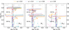 |
Fig. B.1. HRD for the different rotation rates as indicated by line color and style. The left, center, and right panels refer to the Ṁrdw, ṀΓe, and ṀL/M rates, respectively. The gray-shaded region indicates the observed temperature range in the Tarantula Nebula. Data of stars in 30 Doradus are shown in colored symbols, following the same notation as Figure 1. |
For the ṀL/M models with MZAMS = 100 M⊙, rotation begins to change the evolution on the HRD appreciably. Like the Ṁrdw and ṀΓe rates, rotating models with ṀL/M show a steep increase in luminosity at nearly constant Teff at the start of the MS, and the evolution is nearly vertical for ω ≥ 0.6. The ω = 0.6 and ω = 0.8 models have their surface composition dominated by He earlier in the MS compared to the ω = 0.0 and ω = 0.4 models, causing the steeper increase in luminosity. The increased rotation strengthens the mass-loss, and models with ω ≥ 0.6 become WR stars midway through the MS. By the end of the MS, these models have already lost 10 - 15 M⊙ more material than the ω ≤ 0.4 models. By the end of evolution, the rapidly rotating model ends with only 1/2 of the mass of the nonrotating model. On the other hand, the 200 M⊙ model is overall less influenced by rotation than it is by stellar winds, similar to the ṀΓe models. The final masses of rotating and nonrotating models are comparable.
The initial rotation rate at which rotation dominates the evolution depends on the wind prescription, initial mass, and rotation rate. Overall, we found that rotation becomes the dominant factor affecting the evolution on the MS only when ω ≥ 0.6 for Ṁrdw and ṀL/M for stars born with MZAMS ≤ 150 M⊙. For these stars, the variability of when rotational effects become dominant underscores the need for careful selection of wind models. It highlights the complex interplay between the stellar winds, rotation rates, and ZAMS masses. For more massive stars, with MZAMS ≥ 200 M⊙ and all wind prescriptions, mass-loss influences both the HRD evolution and final masses significantly more than rotation does, for the cases explored in this work. This result is in agreement with other works (e.g., Sabhahit et al. 2022), as rotation has a negligible effect on the evolution of VMS (Yusof et al. 2013). A more thorough investigation of the impact of rotation will be conducted in future works.
Pre-SN masses in M⊙ for three different rotation rates.
Appendix C: Merging binary BH formation channels
Having characterized the overall population and formation scenarios of the BHs produced in our simulations in Sections 4.2 and 4.3, we now focus on a particularly interesting subset: the BBHs that experience a gravitational-wave-emitting merger within a Hubble time. Their formation and properties are a direct consequence of the binary evolution explored in the previous sections, which are also relevant to the formation of VMS in dense environments, like that of the Tarantula Nebula.
Binary BHs that coalesce in a Hubble time are the main source of gravitational waves and can provide valuable insights into binary evolution processes. Understanding how these systems form and evolve requires tracing their history through possible formation channels (e.g., Spera et al. 2022). This section details the properties and formational channels of these BHs predicted by our simulations.
In all simulations, the most common formation channel is the so-called ’channel I’, following the definitions given by Broekgaarden et al. (2022), Iorio et al. (2023): the progenitors undergo stable mass transfer before the first BH is formed, and after, evolve through at least one common envelope phase. This occurs in 91% of BBH mergers, regardless of the wind prescription. The second most common channel, occurring in 6% of all BBH mergers, is channel IV, in which the progenitors undergo at least one CE phase before the first BH is formed, and the companion star has been stripped of its envelope before the BH formation.
The frequency of different formation channels is generally very similar for all three simulations, as the majority of merging BBHs originate from progenitors with smaller ZAMS masses, whose evolution is not affected by the enhanced mass-loss treatment presented in this work. The high-mass end of the BBH mergers (with MBH, 1 ≥ 30 M⊙) can arise from VMS progenitors, however, as described in Sect 4.3, which influences the evolutionary pathway to BBH coalescence. For BBH mergers with a primary mass MBH, 1 ≥ 30 M⊙, a common formation channel is channel II. In this channel, the binary system evolves only through stable mass transfer episodes, and occurs in 82%, 47%, and 70% of BBH mergers with Ṁrdw, ṀΓe, and ṀL/M, simulations, respectively. The most common pathway for ṀΓe is channel IV, with exactly one CE episode. The ṀΓe goes through channel IV 48% of the time, while Ṁrdw and ṀL/M experience it just 1.5% and 15% of the time. Finally, there is the possibility that the binaries do not experience any mass transfer episodes, deemed channel 0. This channel arises in 13%, 2%, and 12% of the massive BBH mergers for the Ṁrdw, ṀΓe, and ṀL/M cases.
Very massive primaries (MZAMS, 1 > 140 M⊙) in merging binaries computed with Ṁrdw tend to form with moderately massive secondaries (27 ≲ MZAMS, 2/M⊙ ≲ 47), minor eccentric orbits (e ∈ [0.01, 0.26]), and in close systems, a ∈ [5.8 R⊙, 35.9 R⊙]. Meanwhile, for the simulations with ṀΓe the semi-major axes a ∈ [7.6 R⊙, 63.0 R⊙] are slightly larger, and the orbits are more circularized (e ∈ [0.01, 0.13]). This simulation resulted in a larger population of doubly massive merging systems than the Ṁrdw simulations. For the doubly massive systems computed with ṀL/M have close systems a ∈ [14.3 R⊙, 60.3 R⊙], and a wider variety of eccentricities, e ∈ [0.006, 0.38]. These simulations can produce many doubly massive merging systems, partly due to the remnant masses (see Figure 7).
The most massive primary BHs in the BBH merger population across all three simulations is MBH, 1 ∼ 46  M⊙, originating from progenitor stars with ZAMS masses of 115 M⊙, 108 M⊙, and 210 M⊙ for the Ṁrdw, ṀΓe, and ṀL/M winds, respectively. The ṀΓe and ṀL/M simulations produce up to an order of magnitude more BH primaries with MBH, 1 > 35 M⊙ than the Ṁrdw simulation (see Figure 11). They also yield significantly more massive secondaries, with MBH, 2 ∼ 41.9 M⊙ and 41.7 M⊙, originating from ZAMS masses of 147 M⊙ and 145 M⊙. In contrast, that Ṁrdw simulation produces only a few mergers with secondary BHs above 16 M⊙, and none above 32 M⊙. These differences arise because the stronger winds in the ṀΓe and ṀL/M prescriptions increase mass-loss and reduce stellar radii, lowering the likelihood of binary interactions and stellar mergers (see section 4.2), thereby increasing the number of BBH systems that can later coalesce.
All Tables
Definitions used for different stellar types, adapted from Josiek et al. (2024).
Top table: TAMS mass for each mass-loss rate for a few initial masses. Bottom table: Time spent in the observed temperature range log Teff between 4.75 and 4.6.
Best fit of the stellar tracks within the 68% confidence interval for the massive stars R136a1, R136a2, and R136a3.
Mass estimates of R136a from single and binary stellar mergers for the winds described in this work.
All Figures
|
Fig. 1. Hertzsprung-Russel diagram adapted from Costa et al. (2025) showing stars in the LMC. The green and gray lines show tracks from Costa et al. (2025), that were computed with Z = 0.006 and the standard mass-loss rate. The purple and red stars show objects from B22 (red stars indicate R136a), and the blue and red dots are taken from Schneider et al. (2018) (red dots are WNh stars). The dashed pink line and dash-dotted black line show the ZAMS and TAMS, respectively. The zoomed-in plot shows the most massive stars, and the gray shaded region shows the width of the observed temperature range of VMSs in the LMC. |
| In the text | |
|
Fig. 2. Mass-loss rates predicted for different prescriptions as a function of the mass and luminosity for two |
| In the text | |
|
Fig. 3. Hertzsprung-Russel diagram showing the evolution of stellar tracks computed with the Ṁrdw, ṀΓe, and ṀL/M winds in blue, green, and pink, respectively. The models are shown with ZAMS masses of 300 M⊙ (top), 200 M⊙ (middle), and 150 M⊙ (bottom). The data symbols and shaded gray area are the same as in Figure 1. The black crosses and dots indicate the model location at the TAMS and the start of CHeB. The diagonal dashed gray lines show constant stellar radii as labeled. |
| In the text | |
|
Fig. 4. Maximum radius reached for each ZAMS mass for tracks computed with different mass-loss rates, indicated by the color and marker. The solid lines with blue circles, green diamonds, and pink stars show the maximum radius reached during the evolution for tracks computed with Ṁrdw, ṀΓe, and ṀL/M winds, respectively, and the dashed lines show the maximum radius reached on the MS. The dashed ṀL/M is superimposed on the solid line. The solid gray line shows the ZAMS radius. |
| In the text | |
|
Fig. 5. Kippenhahn diagrams of the stellar tracks computed with the three mass-loss rates with MZAMS = 200 M⊙. The solid blue and green regions show the H and He burning zones, and the purple hatched region shows convective zones. The solid black and navy lines indicate the total mass and the mass of the He core. The red square indicates when the star enters the WR phase (i.e., when |
| In the text | |
|
Fig. 6. Surface abundances of a MZAMS = 200 M⊙ star for three mass-loss rates. The blue, green, and pink shaded bars indicate the time of H, He, and C burning, respectively. |
| In the text | |
|
Fig. 7. Pre-SN mass (markers) and remnant mass (lines) as a function of the ZAMS mass for the three mass-loss rates, indicated by the marker style and color. The horizontal gray lines indicate different fates (PPISN, PISN, and DBH) based on the final He core mass. |
| In the text | |
|
Fig. 8. Averaged percentage of the ZAMS mass accreted onto the primary (left) and secondary (right) per mass bin. The bins are 10 M⊙ each. The colors are the same as in Figure 7. |
| In the text | |
|
Fig. 9. Possible initial masses of R136a1 from single star and stellar merger origins. The shaded areas show the primary and secondary ZAMS masses of stars that merge during evolution and overlap in the HRD with the observed location of R136a1. The blue, green, and pink show results from Ṁrdw ṀΓe, and ṀL/M, respectively. The dashed histograms show the initial mass from single stellar evolution. |
| In the text | |
|
Fig. 10. Black hole number counts for BHs formed from stellar mergers (left) and nonmerging BBHs (right) for the simulations with Ṁrdw (top), ṀΓe (middle), and ṀL/M (bottom). The dashed pink lines indicate BH masses from single stellar evolution. |
| In the text | |
|
Fig. 11. Primary vs. secondary BH masses for BBHs that merge in a Hubble time. The contour plot shows the mergers for binaries with MBH, 1 ≥ 20 M⊙, while the distributions show the full mass range of primary and secondary BH masses on the top and right. The solid blue, dashed green, and dash-dotted pink lines refer to simulations with stellar tracks computed with the Ṁrdw, ṀΓe, and ṀL/M rates, respectively. |
| In the text | |
|
Fig. 12. Number counts of BHs from the simulations with Ṁrdw (left), ṀΓe (center), and ṀL/M (right). The shaded purple shows the result from single stellar evolution. The dashed pink, solid blue, and dash-dotted green lines show results from binary evolution of single BHs, binary BHs that do not merge within a Hubble time, and the resulting BH mass of a BBH merger that merged within a Hubble time, respectively. |
| In the text | |
|
Fig. A.1. The possible initial masses of R136a2 from single star and stellar merger origins. The shaded areas show the primary and secondary ZAMS masses of stars that merge during evolution and overlap in the HRD with the observed location of R136a2. The blue, green, and pink show results from Ṁrdw ṀΓe, and ṀL/M, respectively. The dashed histograms show the initial mass from single stellar evolution. |
| In the text | |
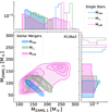 |
Fig. A.2. The same as Figure A.1 but for R136a3. |
| In the text | |
|
Fig. B.1. HRD for the different rotation rates as indicated by line color and style. The left, center, and right panels refer to the Ṁrdw, ṀΓe, and ṀL/M rates, respectively. The gray-shaded region indicates the observed temperature range in the Tarantula Nebula. Data of stars in 30 Doradus are shown in colored symbols, following the same notation as Figure 1. |
| In the text | |
Current usage metrics show cumulative count of Article Views (full-text article views including HTML views, PDF and ePub downloads, according to the available data) and Abstracts Views on Vision4Press platform.
Data correspond to usage on the plateform after 2015. The current usage metrics is available 48-96 hours after online publication and is updated daily on week days.
Initial download of the metrics may take a while.