| Issue |
A&A
Volume 702, October 2025
|
|
|---|---|---|
| Article Number | A254 | |
| Number of page(s) | 10 | |
| Section | The Sun and the Heliosphere | |
| DOI | https://doi.org/10.1051/0004-6361/202347599 | |
| Published online | 24 October 2025 | |
Combined coronal observations of the streamer belt with Metis and EUI instruments on Solar Orbiter
1
INAF – Astrophysical Observatory of Torino, Via Osservatorio 20, 10025 Pino Torinese, Italy
2
Université Paris-Saclay, CNRS, Institut d’Astrophysique Spatiale, F-91405 Orsay, France
3
INAF – Astronomical Observatory of Capodimonte, Salita Moiariello 16, I-80131 Napoli, Italy
4
INAF – Astrophysical Observatory of Catania, Via Santa Sofia 78, I-95123 Catania, Italy
5
University of Firenze, Department of Physics and Astronomy, Via Giovanni Sansone 1, I-50019 Sesto Fiorentino, Italy
6
INAF – Arcetri Astrophysical Observatory, Largo Enrico Fermi 5, 50125 Florence, Italy
7
Predictive Science Inc., San Diego, CA 92121, USA
8
CNR, Institute for Photonics and Nanotechnologies, Via Trasea 7, I-35131 Padova, Italy
9
University of Urbino Carlo Bo, Department of Pure and Applied Sciences, Via Santa Chiara 27, I-61029 Urbino, Italy
10
INFN, Section in Florence, Via Bruno Rossi 1, I-50019 Sesto Fiorentino, Italy
11
Czech Academy of Sciences, Astronomical Institute, Fričova 298, CZ-25165 Ondřejov, Czech Republic
12
University of Wroclaw, Centre of Scientific Excellence Solar and Stellar Activity, ul. Kopernika 11, PL-51-622 Wrocław, Poland
13
University of Padova, Department of Physics and Astronomy, Via Francesco Marzolo 8, I-35131 Padova, Italy
14
ASI, Via del Politecnico snc, I-00133 Roma, Italy
15
Max Planck Institute for Solar System Research, Justus-von-Liebig-Weg 3, D-37077 Gottingen, Germany
16
INAF, Institute of Space Astrophysics and Cosmic Physics of Milan, Via Alfonso Corti 12, I-20133 Milano, Italy
17
Institute of Physics, University of Graz, Universitätsplatz 5, 8010 Graz, Austria
18
INAF – Astronomical Observatory of Trieste, Località Basovizza 302, I-34149 Trieste, Italy
⋆ Corresponding author: This email address is being protected from spambots. You need JavaScript enabled to view it.
Received:
28
July
2023
Accepted:
31
August
2025
Abstract
Context. Comprehensive solar observations from the limb to the extended corona are essential to study the main processes that connect coronal sources of outflows with the heliosphere. In particular, inferring the temperature structure of the solar corona is important to constrain coronal models and to characterise the mechanisms responsible for the plasma heating and acceleration. However, electron temperature is a parameter that is difficult to obtain from direct measurements in the heliocentric range between 3 and 8 R⊙.
Aims. The aim of this work is to show the potentiality of a method of inferring the coronal temperature by exploiting unprecedented combined visible light and extreme-ultraviolet (EUV) observations acquired by Metis and by the Full Sun Imager (FSI) telescope of the Extreme Ultraviolet Imager (EUI) on Solar Orbiter.
Methods. We analysed coordinated observations performed by the two instruments on March 21, 2021. We combined the first image acquired by FSI in the EUV channel at 17.4 nm using its coronagraphic mode with the visible light polarized brightness (pB) Metis data. The intensities measured by Metis and EUI/FSI originate from physical processes that depend differently on electron density and temperature. We propose a method of combining them, allowing us to place constraints on the electron temperature. The electron density, derived from the inversion of the polarized brightness, was used to calculate the expected counts in the FSI passband based on the instrument response function, which is mainly a function of the electron temperature. From the comparison with the measured counts, we were able to infer two different temperature values, corresponding to the two possible solutions, given the analytical shape of the response function.
Results. The electron temperature results at a heliocentric distance of 4.25 R⊙ (i.e. the average height of the Metis/FSI superposition region of the analysed dataset) are (5.3−1.5+2.0) · 105 K and (1.4−0.2+0.3) · 106 K for the east streamer and (5.7−1.4+1.9) · 105 K and (1.4−0.3+0.2) · 106 K for the west streamer. The values derived from the proposed method are consistent with previous estimates in coronal streamers.
Conclusions. For the first time, we have analysed combined coronal observations from EUI and Metis, which has given us a unique opportunity to infer, from their measurements, the physical parameters of the streamer belt. The electron temperature results derived in the present work can be considered as a range of possible values that can constrain this parameter at a coronal height of 4.25 R⊙. The proposed method is reasonable within the limits of the validity of the assumptions considered in this work.
Key words: Sun: corona / Sun: fundamental parameters / Sun: magnetic fields / Sun: UV radiation
© The Authors 2025
 Open Access article, published by EDP Sciences, under the terms of the Creative Commons Attribution License (https://creativecommons.org/licenses/by/4.0), which permits unrestricted use, distribution, and reproduction in any medium, provided the original work is properly cited.
This article is published in open access under the Subscribe to Open model. This email address is being protected from spambots. You need JavaScript enabled to view it. to support open access publication.
1. Introduction
Comprehensive solar observations from the limb to the outer corona are crucial for the study of the main physical transitions and processes that drive and connect coronal sources of outflows with the heliosphere (e.g. Parenti et al. 2022; West et al. 2023, and references therein). Moreover, characterizing the temperature structure of the solar corona is of fundamental importance to constrain and/or assess coronal models that in turn provide information on the physical processes responsible for the bulk-plasma heating and acceleration.
The physical parameters of the coronal plasma have been extensively investigated by analysing ultraviolet (UV) spectral lines (e.g., Wilhelm et al. 2004, 2007; Kohl et al. 2006). In particular, observations from the Ultraviolet Coronagraph and Spectrometer (UVCS) on SOHO (Kohl et al. 1995, 1997) have allowed to achieve important results about the connection between the properties of the solar corona and the solar wind (e.g., Antonucci 2006; Kohl et al. 2006; Antonucci et al. 2012, 2020a; Abbo et al. 2016; Cranmer et al. 2017; Cranmer & Winebarger 2019, and references therein). The electron temperature has been inferred from remote sensing spectroscopic data as well as imaging observations with a variety of diagnostic methods (e.g. Del Zanna & Mason 2018; Parenti et al. 2021, and references therein). Measurements of this parameter have been obtained from line ratios of UV spectral lines from the same element (e.g. Raymond et al. 1997, 2003; David et al. 1998; Li et al. 1998; Parenti et al. 2000, 2003; Marocchi et al. 2001; Bemporad et al. 2003; Uzzo et al. 2004, 2007), but these kinds of measurements are limited to the off-limb corona below ∼2 R⊙. In the extended corona, estimates of the electron temperature have been indirectly derived using the electron density profiles inferred from coronagraphic polarized visible light (VL) brightness measurements, under the assumption of hydrostatic (e.g. Munro & Jackson 1977; Gibson et al. 1999) or hydrodynamic equilibrium (e.g. Lemaire & Stegen 2016). More recently, narrow-band coronal imaging in VL or near-infrared lines, performed either from space (e.g. Gopalswamy et al. 2021) or during total solar eclipses (e.g. Habbal et al. 2021; Boe et al. 2022, 2023; Del Zanna et al. 2023), have been used to infer the electron temperature up to ∼3–4 R⊙, as well as to characterize the line-of-sight (l.o.s.) distribution of the electron temperature within different coronal structures such as streamers and coronal holes, under the assumption of the ionization equilibrium. In this work we explore the feasibility of an alternative method of inferring an estimate of the electron temperature by analyzing multi-band observations acquired by Metis (Antonucci et al. 2020b; Fineschi et al. 2020) and the Extreme Ultraviolet Imager (EUI, Rochus et al. 2020) instruments aboard the Solar Orbiter spacecraft (Müller et al. 2020). In particular, we analyze the first coronagraphic images acquired with the Full Sun Imager (FSI) telescope of EUI in the 17.4 nm bandpass (see Auchère et al. 2023a), which allows observations at coronal heights not usually reachable with a disk imager due to instrumental stray-light contamination. These observations are combined with those obtained by the Metis coronagraph in the VL and H I Lyman-α channels, focusing on the analysis of two streamer regions. The paper is organised as follows. In Section 2, the Metis and EUI/FSI observations analysed in this study are described in detail; the different physical processes responsible for the emission detected by the two instruments and their dependence on the plasma physical parameters are described in Section 3. In Section 4 we explain the method used to derive the plasma parameters in streamers; Section 5 is dedicated to the discussion of the results, the assumptions at the base of the proposed method, and possible future developments of this work.
2. Metis and EUI observations
The Metis and EUI/FSI observations considered in this paper were obtained on March 21, 2021, during Solar Orbiter’s cruise phase, when the spacecraft was at a distance from the Sun of ∼0.68 au and with heliographic longitude of ∼110°E. We used the FSI channel of EUI in the coronagraphic mode, which allows to obtain stray-light free off-limb observations. In particular, FSI includes a movable occulting disk located at the entrance door of the instrument (Rochus et al. 2020). This device allows imaging of the faint Fe IX/Fe X emission beyond 2 R⊙, where the coronal signal acquired in the nominal FSI disk mode is largely dominated by instrumental stray light. We refer the reader to Auchère et al. (2023a) for a detailed description of the FSI occultation system and the observation campaigns performed in this particular configuration. It is worth noting that the coronagraphic mode of EUI is feasible only for S/C distances down to 0.45 au.
In this paper, we use the first science-grade image obtained by FSI in coronagraphic mode. It was acquired at 00:45:45 UT on March 21, 2021 with an exposure time of 640 s. FSI has an average plate scale of 4.46″/pixel corresponding to ∼2200 km/pixel on the plane of the sky when Solar Orbiter is at a distance of 0.68 au from the Sun and a full field of view (FOV) of 3.8° that corresponds to 9.7 R⊙ along the equatorial plane. The spatial resolution is twice the plate scale. The data were dark-subtracted and despiked using the procedure described in Auchère et al. (2023a). The DOI of the EUI Data release for the analysed observations is Data Release 6 (Kraaikamp et al. 2023). Metis provides simultaneous observations of the outer solar corona in VL polarized brightness (pB) and UV, imaging the electron-scattered K-corona and the neutral hydrogen Lyman-α line (121.6 nm) intensity, respectively. Starting at 03:00 UT on March 21, 2021, Metis performed a series of observations aimed at studying the evolution of the large-scale corona and the overall configuration of the neutral-hydrogen and electron components of the coronal plasma (see Antonucci et al. 2020b, for more details). Metis data consist of sequences of four polarized VL images, obtained by averaging on board 14 frames at the same polarization angle and with an integration time of 30 s (for a total effective exposure time of 420 s), acquired in parallel with UV images with exposure time of 60 s. The plate scales of Metis detectors are of 10.14″/pixel and 20.4″/pixel for the VL and UV channels, respectively. The spatial resolution is twice the plate scale. To improve the statistics, all acquisitions were carried out with a 4 × 4 pixel binning, corresponding to ∼20 000 km/pixel in the VL channel and ∼40 000 km km/pixel in the UV channel. The Metis FOV ranged from ∼4 R⊙ at the edge of the internal occulter up to ∼7.4 R⊙ along the equatorial plane. Both sets of VL and UV images were processed and calibrated in the manner described in Romoli et al. (2021) and Andretta et al. (2021), with the most up-to-date radiometric calibration available (see De Leo et al. 2023, 2025). The standard data processing applied includes the subtraction of dark and bias frames, correction for detector flat-field and optical vignetting, normalization by the exposure time, and radiometric calibration. In addition, images of each VL polarization sequence were combined together according to the Müller formalism to derive a single pB image corresponding to an effective exposure time of 1680 s. Unfortunately, there are no Metis observations simultaneous with the coronagraphic FSI acquisition mentioned above. Hence, for the present analysis the closest available Metis data have been considered, i.e., the first VL pB and UV Lyman-α images acquired on March 21, at 03:00 UT. In the 2.25 hours between FSI and Metis observations, however, no solar eruptive events occurred and rotational and orbital effects (due to the solar rotation and/or the relative motion between Solar Orbiter and the Sun) can be neglected; therefore, the coronal structure observed by the two instruments can be considered substantially the same. On the other hand, it is worth mentioning that on March 20, i.e. the day before the analysed observations, a coronal mass ejection (CME) occurred starting at 01:25 UT, which was followed by a series of minor eruptions lasting approximately all the day. This activity has been detected by both SOHO/LASCO and STEREO-A/SECCHI suites of coronagraphs, but not by Metis, whose external door has been kept closed from 23:30 UT on March 17 until 23:50 UT on March 20. Although the CME has certainly caused a disruption of the global configuration of the solar atmosphere and a subsequent rearrangement of its overall magnetic-field structure, in the following hours the corona has again attained quasi-static conditions. No other major eruptions were detected until 11:00 UT on March 21. Figure 1 reports composites between the FSI 17.4 nm image acquired at 02:46:43 UT using the nominal disk mode, showing the Fe IX/Fe X emission in the lower corona below 1.85 R⊙, the image in the same passband obtained using the FSI coronagraphic mode described above, showing the coronal emission from the same ions between 1.85 and 4.25 R⊙, and the Metis pB (left panel) and UV Lyman-α (right panel) images acquired at 03:00 UT, showing the electron and neutral-hydrogen plasma components of the outer corona above 4.25 R⊙. It is worth noting that by combining the two instruments, it is possible to image the whole corona from the limb up to about ∼7.4 R⊙ along the equatorial plane. In particular, FSI and Metis fields of view overlap in a region ranging between ∼4 − 4.5 R⊙ (marked by the dotted white circles in Figure 1) where co-spatial data are available. We find a remarkable similarity in the radial emission distribution in EUI/FSI and Metis images, especially in the equatorial regions above the western and eastern limbs, where the streamer belt appears to be more structured. Looking at this region in more detail, we can study the coronal features starting from the FSI FOV up to the Metis one: in the left panel of Figure 2, in particular, a wavelet-optimized-whitening filter (WOW; Auchère et al. 2023b) has been applied to highlight coronal structures in the Metis pB image. The right panel of Figure 2 shows the magnetic extrapolation of the field lines obtained by applying the 3D MHD MAS model developed by Predictive Science Incorporated (PSI; e.g., Mikić et al. 2018, and references therein). The photospheric boundary conditions used for the extrapolation are given by synoptic magnetic-field measurements from the Helioseismic and Magnetic Imager (HMI) on board the Solar Dynamics Observatory (SDO, Scherrer et al. 2012) during Carrington rotation 2242. The closed and open fields are well structured up to the outer corona where the field becomes more radially aligned. The comparison between the observations and the extrapolated field lines allows us to identify the closed magnetic structures in a streamer belt typical of the solar minimum phase.
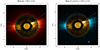 |
Fig. 1. Composite of FSI 17.4 nm images obtained on March 21, 2021, on disk (at 02:46:43 UT, below 1.85 R⊙) and in coronagraphic mode (at 00:45:45 UT, between 1.85 and 4.45 R⊙), and Metis polarized-brightness (pB, left) and UV Lyman-α (right) images acquired at 03:00 UT, above 4.45 R⊙. The dotted white circles mark the inner (4.05 R⊙) and outer (4.45 R⊙) limits of the overlapping portion of FSI and the Metis fields of view. The streamer regions considered in the analysis are shown by the two angular sectors delimited by the dotted lines. |
 |
Fig. 2. Left: Same data as in the left panel of Figure 1, but in this case Metis pB and EUI/FSI images have been enhanced using the WOW filter (see the text). Right: Extrapolation of the magnetic field lines with the 3D MHD model developed by Predictive Science Inc. (PSI) for the date of March 21, 2021, as seen from Solar Orbiter’s point of view. |
3. Formation of the VL and EUV band emissions
The intensities measured by Metis and EUI/FSI at different wavelengths originate from physical processes that depend in a distinct way on electron density and temperature. Under proper assumptions, it is therefore possible to exploit co-spatial data from the two instruments to derive information and/or place constraints on the physical properties of the emitting plasma. In particular, in this work we focus on the analysis of Metis VL pB and EUI/FSI 17.4 nm data, because emission in these passbands has a rather clear dependence on the plasma electron density and temperature.
The VL pB is due to Thomson scattering of the photospheric light by free electrons in the corona (K-corona), so it is a function of the electron density, ne. The relationship between the pB and the electron density can be written as follows (see van de Hulst 1950):
![Mathematical equation: $$ \begin{aligned} I_{pB} \propto \int _{\rho }^{\infty } n_e(r)\,[A(r) - B(r)]\,\frac{\rho ^2 dr}{r\sqrt{r^2 - \rho ^2}}, \end{aligned} $$](/articles/aa/full_html/2025/10/aa47599-23/aa47599-23-eq5.gif) (1)
(1)
where A(r) and B(r) are geometrical factors, r is the heliocentric distance, and integration is performed along the line of sight whose projected distance on the plane of the sky is given by ρ. In the local spherical symmetry approximation, which means that the electron density depends locally only on the heliocentric distance, ne = ne(r), van de Hulst (1950) also provided a simple and widely adopted method of inferring the coronal electron density from the measured pB by inverting Eq. (1). As for the FSI EUV emission, the spectral lines dominating the 17.4 nm passband are emitted by Fe IX/Fe X ions following collisional excitation (even if resonant scattering of Fe IX line at 17.1 nm may also play a role; see, e.g., Schrijver & McMullen 2000); the emitted intensity for each iron line, integrated along the l.o.s., can be written as:
 (2)
(2)
where AFe is the iron abundance and G(Te, ne) the contribution function that combines all atomic parameters characterizing the line transition. In particular, G(Te, ne) is strongly peaked in temperature because of the element ionization fraction, but it also slightly depends on the electron density because of the collisional excitation rates. The coronal H I Lyman-α emission originates primarily from the resonance scattering of chromospheric radiation by neutral hydrogen atoms in the corona (Gabriel 1971) and is a function of electron density, electron temperature and the neutral hydrogen kinetic temperature, as well as of the chromospheric Lyman-α line intensity and profile. Moreover, it depends on the solar-wind outflow velocity through the Doppler dimming effect (Hyder & Lites 1970; Withbroe et al. 1982; Noci et al. 1987), which consists of a decrease in the scattered intensity as a function of the solar-wind velocity. In the present analysis, UV images acquired by Metis are only used for comparison purposes. A full inversion of these data through the Doppler-dimming technique (see, e.g., Romoli et al. 2021; Antonucci et al. 2023) is outside of the scope of this paper. Figure 3 (top panel) shows the latitudinal distribution of the measured intensity in the three bands (Metis VL pB and HI Lyman-α, and FSI 17.4 nm) in the overlapping region as a function of the polar angle (PA, measured counterclockwise from the north pole). In the bottom panel, the latitudinal profile obtained by averaging the intensities over the height range between 4.05–4.45 R⊙and 1-degree wide angular sectors is reported. The uncertainties, shown as error bars in the plot, have been estimated by propagating the Poissonian statistical error on the measured counts. For Metis, uncertainties arising from the calibration process have also been considered, including those affecting calibration data such as bias and dark images, flat field, vignetting function, and radiometric coefficients. According to De Leo et al. (2023, 2025), and Liberatore et al. (2023), uncertainties in the radiometric calibration of Metis are of the order of 7% and 15% for the VL and UV channels, respectively. For FSI, a flat 30% error has been adopted as an estimate of the calibration uncertainty (EUI team private communication). Although the uncertainties affecting FSI and Metis Lyman-α data in the equatorial region are larger than both the uncertainty affecting the VL pB and most of the small-scale variations in the measured emissions, some of the intensity features that can be identified as peaks in the profiles have corresponding counterparts in the three bands; it is the case, for instance, of the main peak in the east streamer around PA ∼ 90° or the two peaks in the west streamer around PA ∼ 265° and PA ∼ 292.5°. These features mark the continuity, from the inner to the outer layers, of the coronal structures which are organized according to the magnetic-field topology, as is also depicted in Figure 2. On the other hand, there are also significant discrepancies that are likely caused by different emission processes (due to either temperature or density l.o.s. distribution effects) and/or to a temporal effect, since the observations are almost at the same time, but not simultaneous. For instance, the FSI intensity profile (grey line) exhibits several local enhancements especially in the western streamer which appears to be more structured that are absent or only partially visible in the Metis profiles. The radial profiles derived along the central positions of the eastern and western streamers identified by the main peaks in the pB latitudinal distribution (at PAs of 90° and 292.5°, respectively) are shown in Figure 4. They have been obtained by averaging the measured intensities over a 2-degree wide angular sector around the center of the streamers; in addition, they have been normalized to the average value in the superposition region (between 4.05–4.45 R⊙) to improve the comparison (for this reason, they are also reported in arbitrary units). The Metis pB and H I Lyman-α profiles (red and blue curves, respectively) exhibit very similar trends, as was expected, since the VL and Lyman-α intensities are both approximately proportional to the integral of electron density distribution along the l.o.s. as it could be expected for the slow solar-wind flow velocities typical of the regions in the core of equatorial helmet streamers (see, e.g. Abbo et al. 2016, and references therein). The Lyman-α profile is characterized, however, by a slightly steeper decrease although not a significant one due to the uncertainties that could be ascribed to the increasing outflow velocity of the H I atoms, which in turn causes the Doppler dimming of the Lyman-α resonantly scattered radiation. The FSI intensity profile (solid grey line) is very steep at coronal heights from 2 to 4 R⊙, where it decreases by three orders of magnitude.
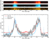 |
Fig. 3. Top: Intensity maps of the overlapping region in the height range ∼4–4.5 R⊙ for the three bands: Metis/VL channel, pB emission, in red (higher row), the Metis/UV channel in blue (central row) and the EUI/FSI 17.4 nm band in yellow (lower row). Bottom: Latitudinal profiles (in arbitrary units) of Metis pB (red line), of Lyman-α intensity (blue line) and of FSI 17.4 nm intensity (grey line) obtained by averaging the data in the overlapping region. The profiles are normalised to their maximum value (the values including the error bars are greater than 1). |
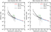 |
Fig. 4. Radial profiles of Metis pB (red lines), H I Lyman-α intensity (blue lines), FSI Fe IX/Fe X 17.4 nm intensity (thick grey lines), and the square root of FSI intensity (thick black lines) for the eastern streamer (left panel) and the western streamer (right panel). In order to be comparable, all profiles are normalized to their average value in the overlapping region between 4.05 and 4.45 R⊙, indicated in plots by the vertical green arrows. |
The comparison of the FSI and Metis data is also useful to test if the FSI emission is dominated by collisional processes. This is done by comparing the square root (as the intensity is proportional to ne2) of the FSI (thick black line) to the VL Metis profiles (red line), as shown in Figure 4: it turns out that they are more consistent in terms of spatial trend with those derived from Metis data at larger heights. This could be an indication that the emission detected by FSI at these coronal heights is mainly due to collisional excitation, since its dependence seems to be nearly proportional to ne2. On the other hand, we cannot rule out that a contribution from resonant scattering is also present, especially approaching the outer limit of the FSI FOV above ∼4 R⊙, where the uncertainties are also larger. In the following, we assumed as a first approximation that this contribution is negligible.
4. Data analysis
4.1. Electron density
The coronal electron density, ne, was derived from the polarized brightness data acquired by the Metis VL channel by using the standard inversion technique developed by van de Hulst (1950), assuming local spherical symmetry. This assumption can be considered fairly appropriate in coronal regions such as coronal holes and along the central axis of streamers, where the latitudinal and azimuthal variations in the electron density can be considered weaker than its radial gradient.
The ne maps obtained for the eastern and western streamers are reported in the left and right top panels of Figure 5, respectively. The bottom panel shows the electron density radial profiles, derived by averaging the pB in the two regions marked with the thin vertical lines in the top panels. Uncertainties in the density profiles (reported in the bottom panel of Fig. 5 as error bars on the red and orange curves) were obtained by considering, in the inversion of Eq. (1), the minimum and maximum pB values according to the uncertainty affecting Metis pB data.
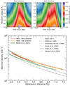 |
Fig. 5. Top: Electron density maps derived from Metis pB data in the two regions surrounding the east and west equatorial streamers, centered, respectively, at PA = 90° (left) and at PA = 292.5° (right). The thin vertical lines mark the regions considered in the study. Bottom: Electron density radial profiles obtained from this analysis, compared with the streamer profile obtained from Metis first-light data (green by Romoli et al. 2021) and with other density profiles for equatorial and mid-latitude streamers reported in the literature, as is indicated in the legend (see also the text). |
The resulting densities were compared with several density profiles taken from the literature, obtained for equatorial or mid-latitude streamers around solar activity minimum: the profile derived by Romoli et al. (2021) for an equatorial streamer observed by Metis in May 2020 (green line); the model by Saito et al. (1977) corresponding to the declining phase of the solar cycle approaching solar minimum (dotted line); the quiet-corona model by Withbroe (1988) (dashed line); the profile inferred by Guhathakurta et al. (1999) for the heliographic current sheet during the declining phase of solar activity (small-dotted line); the profile derived by Gibson et al. (1999) from MLSO/Mk-3 and LASCO/C2 measurements in the equatorial streamer belt between 2 and 4 R⊙ (extrapolated up to the heights considered in this work; long-dashed line); the density profile derived by Hayes et al. (2001) from LASCO/C2 data of a near-equatorial streamer during the rising phase of solar activity (dash-dotted line); the streamer densities values reported by Frazin et al. (2003), obtained with tomography applied to LASCO/C2 data (solid line); and the equatorial density profile inferred by Vásquez et al. (2003) (dash-triple-dotted line). It is worth noting that the density profiles obtained in the present analysis are comparable with some of the profiles reported in the literature, in terms of both absolute values and radial trends; for instance, the profiles of Withbroe (1988), Hayes et al. (2001), and Frazin et al. (2003). On the other hand, the scatter of the reported profiles over a factor greater than 2 is an indication of the large variability of the electron density values for different coronal structures observed approximately near the solar minimum phase.
4.2. Emission measure and electron temperature
To estimate the electron temperature, Te, in the Metis and FSI overlapping region, we adopted a method similar to the loci technique (see, e.g., Guennou et al. 2012, and references therein). We computed the expected FSI 17.4 nm count rates at different latitudes in the height range between 4.05–4.45 R⊙ as a function of Te, and then we constrained these results with the observations, as is described in the following.
The emission measure (EM) was computed by integrating the electron density profile derived with Metis along the l.o.s., according to the definition:
 (3)
(3)
We derived an EM map (see Figure 6, top panel) by integrating along a l.o.s. extending ±10 R⊙ from the plane of the sky. In particular, we assumed that for each point on the plane of the sky and within the Metis FOV, the electron density profile along the l.o.s. is equal to the density profile along the radial direction through that point, extrapolating it up to 10 R⊙, since Metis pB data extend up to ∼7.4 R⊙ in the equatorial regions. We verified that for a heliocentric distance of 4.25 R⊙ (i.e. the average height of the Metis/FSI superposition region) this integration length gives an EM that is at least 99% of the asymptotic value that would be obtained by extending the integration up to very large distances from the plane of the sky. From Eq. (2), the column EM is derived from the optically thin VL brightness measured with Metis. Given the estimate of the EM, the number of counts per unit time (units of DN/s) expected from FSI can be calculated using the relationship:
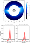 |
Fig. 6. Top: Map of EM computed from the electron density derived with Metis, as is described in the text. Bottom: Comparison between the count rates measured in the FSI 17.4 nm passband (horizontal grey bands) and the expected count rates (red bands) calculated from the EM according to Eq. (4), in the eastern (left panel) and western (right panel) streamers (the values are shown with the corresponding uncertainties, as is explained in the text). |
 (4)
(4)
where R(Te, ne), the response function of the FSI 17.4 nm passband, includes the spectral sensitivity of the instrument, the element abundance and the contribution functions of all the spectral lines in the passband. For the present analysis, the response function was computed for the density values derived from Metis and by using atomic parameters, ionization balances from the CHIANTI atomic database (version 10.1; see Dere et al. 1997, 2023; Del Zanna et al. 2021). We have considered two values of iron abundance: the photospheric abundances of Asplund et al. (2021) and the value provided by CHIANTI derived from the photospheric abundances corrected for low first ionization potential (FIP) elements (FIP ≤ 10 eV) by a factor of 100.5 (see Dere et al. 2023). It is worth noting that this computation can be applied under the assumptions that the plasma along the l.o.s. is isothermal and in ionization equilibrium, as is discussed in Section 5. We performed the calculation in two latitudinal ranges between ±15° from the streamer centers, averaging the EM over 2-degree wide angular sectors in the Metis/FSI overlapping region. The result is a set of curves providing the expected count rates in the FSI 17.4 nm passband as a function of Te only. As an example, the curves obtained at the center of the two streamers are reported in Figure 6 (bottom panels). The red bands correspond to the minimum and maximum expected count rates computed by taking into account the uncertainties affecting the EM due to electron density errors, see Section 4.1, and the two considered values of iron abundance. The horizontal grey band corresponds to the count rates observed in the FSI 17.4 nm passband, averaged over the same angular sector and considering the associated uncertainties. By comparing expected and measured count rates, it is possible to infer two values (corresponding to the intersections of the red and grey bands, as is shown in Fig. 6, bottom panels), each range providing an average temperature value and an associated error. In the following, we refer to the lower temperature values as the ‘cold’ solutions and to the higher ones as the ‘hot’ solutions.
Figure 7 reports the resulting temperature values as a function of the angular distance from the streamer central PA, for the eastern (orange lines) and western (red lines) streamers. The cold and hot temperature solutions are identified by solid and dashed lines, respectively. The error bars include all the uncertainties of the analysis. The figure also shows that the derived temperature does not appear to change significantly within the streamer regions, implying that the denser streamer plasma contributing to the FSI emission could be associated with almost uniform temperature conditions. Note that the larger uncertainties characterizing the cold solutions may be due to the presence of a plateau around log Te = 5.4 in the FSI response function (see Fig. 6).
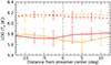 |
Fig. 7. Electron temperature (in logarithmic scale) as a function of the angular distance from the center of the streamers (marked with the vertical dash-dotted line) for the eastern streamer (orange lines) and the western streamer (red lines). The lower (cold) and higher (hot) temperature solutions are identified by solid and dashed lines, respectively. |
5. Discussion
In this paper, we have presented a method of estimating the electron temperature in the outer corona by combining multi-band Solar Orbiter observations from EUI/FSI, obtained in the 17.4 nm channel using an innovative coronagraphic mode that allows us to detect the EUV Fe IX/Fe X emission in the outer corona, and Metis, in particular in the VL pB. The electron density derived from the inversion of Metis pB data was used to estimate the column EM in the region where the fields of view of the two instruments overlap (between ∼4–4.5 R⊙ in the case of the considered observations performed on March 21, 2021) within two bright equatorial streamers visible above the eastern and western limbs at that time. The estimated EM was then used to calculate the expected counts in the FSI passband based on the instrument response function, which is mainly a function of electron temperature, and through comparison with the measured counts we were able to infer two different temperature values, corresponding to the two possible solutions given the analytical shape of the response function.
We report in Figure 8 the average electron temperatures derived for the two streamers in the Metis/FSI superposition region (at the representative height of 4.25 R⊙), obtained with the method described in this work (western streamer in red, eastern streamer in orange). In particular, the values obtained are ((5.3 K and (1.4
 K for the east streamer and (5.7
 K and (1.4
 K for the west streamer.
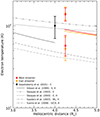 |
Fig. 8. Electron temperatures values derived for the western (red) and eastern (orange) streamers region (at the representative height of 4.25 R⊙), obtained with the method described in this work (open circles: cold solutions; filled circles: hot solutions, see the text for details). The thick coloured lines show the electron temperature profiles derived from the inversion of the ne curves obtained from Metis data assuming hydrostatic equilibrium. The inferred values are compared with others from the literature, as reported in the plot legend and in the text. In particular, we show Te profiles for equatorial (E), mid-latitude (ML) streamers, and the streamer and/or coronal-hole boundary (S/CH). Profiles with H in the legend were derived from the corresponding density profiles assuming hydrostatic equilibrium. |
These values are compared with some literature Te profiles for equatorial and mid-latitude streamers obtained in a time period close to the solar minimum activity: values for an equatorial streamer by Gibson et al. (1999) (solid black line), profiles by Vásquez et al. (2003) for an equatorial streamer (dashed-triple dotted) and for a hydrostatic model (dotted line); a full black dot is derived from the measurements by BITSE instrument published by Gopalswamy et al. (2021) for equatorial regions; a dash-dotted black line shows the values by Spadaro et al. (2007) for the axis of a mid-latitude streamer; the dash-dotted grey line shows the values by Susino et al. (2008) for the streamer and coronal hole boundary (it is shown the average obtained by two regions).
In addition, we derived the electron temperature profiles from the inversion of the ne curves obtained from Metis data assuming hydrostatic equilibrium (as described, e.g., in Gibson et al. 1999) and they are shown as solid coloured lines in Figure 8. It is worth noting that Te values shown in this plot vary within a factor of 3.
We notice that the cold solutions are comparable with profiles obtained by Spadaro et al. (2007) and Susino et al. (2008) in the streamer axis regions. However, other studies with results obtained at 2.7–2.8 R⊙ and up to 3 R⊙ show that Te values above 1 MK, corresponding to the hot solutions of the present work, can be justified at the height of 4 R⊙ by taking into account a slow decrease in the temperature as a function of heliodistance. In particular, Fineschi et al. (1998) obtained a value of Te = (1.1 ± 0.3)⋅106 K, by measuring with UVCS the profile of the electron scattered HI Lyman-α in an equatorial streamer. Boe et al. (2023) found that in the low corona, below about 1.3 R⊙, there are wide distributions in the Te values, but beyond that distance, the corona seems to be almost isothermal. The analysed quiescent streamers at the equator show a constant temperature of about 1.4–1.65 MK up to 2.8 R⊙. It is noteworthy that SOHO/UVCS observations of EUV coronal lines in quiescent streamers, between 1.4 and 3 R⊙, also indicate a constant ionization temperature of about 1.4 MK, as has been reported by Del Zanna et al. (2018). The inferred Te results (cold and hot solutions) of the present work can be considered as a range of possible values that can constrain this parameter at a coronal height of about 4 R⊙.
However, in order to apply the proposed method two important assumptions have been implicitly made, which deserve further discussion. The first and more critical one is the ionization equilibrium that is assumed in the calculation of the contribution functions going into the FSI instrument response function R(Te, ne) (see Eqs. (3) and (4)). One way to evaluate possible departures from ionization equilibrium is through a comparison of the characteristic time for coronal expansion, given by ![Mathematical equation: $ \tau_{\mathrm{exp}}=[(\frac{v}{n_e}) \frac{dn_e}{dr}]^{-1} $](/articles/aa/full_html/2025/10/aa47599-23/aa47599-23-eq13.gif) , where v is the solar-wind outflow velocity, with the collisional ionization and recombination timescales (see, e.g., Withbroe et al. 1982) for the relevant atomic species, in our case the Fe X and Fe IX ions. These timescales can be computed as
, where v is the solar-wind outflow velocity, with the collisional ionization and recombination timescales (see, e.g., Withbroe et al. 1982) for the relevant atomic species, in our case the Fe X and Fe IX ions. These timescales can be computed as  and
and  , where αion and αrec are the collisional ionization and recombination rates, which depend on the electron temperature. Figure 9 reports the Fe X and Fe IX ionization and recombination timescales as a function of heliocentric distance, calculated using the electron density profile ne(r) derived from Metis data in the west streamer and the collisional rates computed with CHIANTI atomic database (version 10.1; see Dere et al. 1997, 2023; Del Zanna et al. 2021) for the electron temperature obtained assuming hydrostatic equilibrium. The vertical bars mark the variation in the timescales computed at 4.25 R⊙with the two temperature values derived in the present analysis (cold solution, ∼0.5 MK, and hot solution, ∼1.6 MK). They are compared with the characteristic coronal expansion time at 4.25 R⊙ estimated using the same density profile and three values of the solar-wind outflow velocity in the range 20–100 km s−1, which can be considered representative of the dynamical conditions of the coronal regions above the cusp of equatorial streamers at ∼4–4.5 R⊙ (see, e.g., Abbo et al. 2016, and references therein).
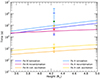 |
Fig. 9. Fe IX (dark colors) and Fe X (light colors) timescales for ionization (blue lines), recombination (purple lines), and collisional excitation (yellow lines), compared with solar-wind expansion times computed at 4.25 R⊙ for three representative values of the outflow velocity (20 km s−1, green dot; 50 km s−1, orange dot; 100 km s−1, red dot). The vertical bars mark the variation in the timescales computed at 4.25 R⊙ with the two temperature values derived in the present analysis (cold solution, ∼0.5 MK, and hot solution, ∼1.4 MK). See the text for details. |
It is evident that for the plasma conditions resulting from the present analysis, and at the considered height in the corona, the coronal expansion time is basically comparable with the ionization and recombination timescales of both Fe X and Fe IX ions, and the situation is at the limit of applicability of the hypothesis of ionization equilibrium.
However, even if we cannot rule out that the ionization balance of these atomic species could already be in a frozen-in state, especially at larger solar-wind flow velocities, the assumption of ionization equilibrium could be still considered fairly reasonable in first approximation, at least in this specific case.
On the other hand, previous estimates of the freeze-in distance for heavy ions such as Fe X, Fe XI, and Fe XIV obtained using narrow-band filter observations of the corona during total solar eclipses (see, e.g., Habbal et al. 2010, 2011, 2021; Boe et al. 2018, 2023) show that the height where there are not enough collisions to keep the equilibrium may occur already at ∼2 R⊙.
In any case, we would like to note that Boe et al. (2018) found that in the regions where the resonant scattering dominates, it is possible to use visible-light observations of Fe10+, Fe13+ ions as a proxy to estimate freeze-in distances. In particular, they obtain in coronal holes and helmet-streamers distances of 1.25–2 R⊙ and 1.45–2.2 R⊙, respectively. However, theoretical freeze-in heights can be considerably larger in pseudostreamers (Shen et al. 2018). Similarly, simulations of the solar wind have shown that freeze-in distances for other ions of C, O, and Fe in coronal-hole wind can range between 1–2 R⊙, while in equatorial-streamer-belt wind ions may evolve beyond 5 R⊙ (e.g., Ko et al. 1997; Landi et al. 2012a,b; Gilly & Cranmer 2020).
We point out that in a situation of frozen-in charge states, the temperatures derived in this work could be decoupled from the local electron temperature and mostly related to the ionization and recombination temperatures of Fe IX/Fe X ions and indicative of the thermal conditions of the plasma at the freeze-in height. In this case the results obtained in this work can be considered as an upper limit of the local electron temperature.
The other underlying assumption in the method is that of isothermal plasma along the l.o.s., implied by the use of the column EM derived from the optically thin VL brightness measured with Metis. On the one hand, the electron temperature may vary along the l.o.s. because of the presence of different coronal structures at different plasma temperatures, as well as because the temperature does indeed decrease with increasing heliocentric distance moving away from the plane of the sky. However, since we are dealing with the core of two bright equatorial streamers, it is likely that the bulk of the emission, both in the VL and EUV, is coming from the denser plasma confined in the portion of the l.o.s. crossing the streamer, where we do not expect a mixture of small-scale structures at very different temperatures, while contribution of low-density regions outside the streamer could be negligible. In addition, empirical models (see, e.g., Withbroe 1988; Vásquez et al. 2003; Lemaire & Stegen 2016) as well as eclipse observations (see, e.g., Habbal et al. 2021; Boe et al. 2023; Del Zanna et al. 2023) support the hypothesis that the rate of decrease in the electron temperature in most solar wind sources is generally slow, especially in the outer corona, and the l.o.s. temperature variation inside coronal structures may be negligible.
The present work has the goal of showing the potential of a method of estimating the electron temperature in the outer corona with EUI and Metis instruments. The dataset analysed in this study is the first acquired in the coronagraphic mode by the FSI/EUI telescope in coordination with the Metis instrument. More recently, there are other datasets of combined observations that also include the He II 304 narrow-band channel of FSI. The analysis of these observations in three bands (Metis VL and FSI 174, 304) could improve the application of the method to distinguish the two values of temperature as discussed by Guennou et al. (2012). However, the validity of the ionization equilibrium is indeed an aspect to be further investigated by applying the same method to other combined observations acquired when the overlapping FOV of the instruments covers heights below 4 R⊙, where the ionization equilibrium assumption is less critical.
Acknowledgments
Solar Orbiter is a space mission of international collaboration between ESA and NASA, operated by ESA. Metis was built and operated with funding from the Italian Space Agency (ASI), under contracts to the National Institute of Astrophysics (INAF) and industrial partners. Metis was built with hardware contributions from Germany (Bundesministerium für Wirtschaft und Energie through DLR), from the Czech Republic (PRODEX) and from ESA. Metis team thanks the former PI, Ester Antonucci, for leading the development of Metis until the final delivery to ESA. Moreover, the authors thanks EA for useful comments and suggestions to improve the discussion of the results. The EUI instrument was built by CSL, IAS, MPS, MSSL/UCL, PMOD/WRC, ROB, LCF/IO with funding from the Belgian Federal Science Policy Office (BELSPO/PRODEX PEA C4000134088); the Centre National d’Etudes Spatiales (CNES); the UK Space Agency (UKSA); the Bundesministerium für Wirtschaft und Energie (BMWi) through the Deutsches Zentrum für Luft- und Raumfahrt (DLR); and the Swiss Space Office (SSO). CHIANTI is a collaborative project involving George Mason University, the University of Michigan (USA), University of Cambridge (UK) and NASA Goddard Space Flight Center (USA). P.H. was supported by the Czech Funding Agency with grant No. 22-34841S and by the program “Excellence Initiative – Research University” for years 2020-2026 at University of Wrocław, project no. BPIDUB.4610.96.2021.KG.
References
- Abbo, L., Ofman, L., Antiochos, S. K., et al. 2016, Space Sci. Rev., 201, 55 [NASA ADS] [CrossRef] [Google Scholar]
- Andretta, V., Bemporad, A., De Leo, Y., et al. 2021, A&A, 656, L14 [NASA ADS] [CrossRef] [EDP Sciences] [Google Scholar]
- Antonucci, E. 2006, Space Sci. Rev., 124, 35 [Google Scholar]
- Antonucci, E., Abbo, L., & Telloni, D. 2012, Space Sci. Rev., 172, 5 [NASA ADS] [CrossRef] [Google Scholar]
- Antonucci, E., Harra, L., Susino, R., & Telloni, D. 2020a, Space Sci. Rev., 216, 117 [CrossRef] [Google Scholar]
- Antonucci, E., Romoli, M., Andretta, V., et al. 2020b, A&A, 642, A10 [NASA ADS] [CrossRef] [EDP Sciences] [Google Scholar]
- Antonucci, E., Downs, C., Capuano, G. E., et al. 2023, Phys. Plasma, 30, 022905 [Google Scholar]
- Asplund, M., Amarsi, A. M., & Grevesse, N. 2021, A&A, 653, A141 [NASA ADS] [CrossRef] [EDP Sciences] [Google Scholar]
- Auchère, F., Berghmans, D., Dumesnil, C., et al. 2023a, A&A, 674, A127 [NASA ADS] [CrossRef] [EDP Sciences] [Google Scholar]
- Auchère, F., Soubrié, E., Pelouze, G., & Buchlin, É. 2023b, A&A, 670, A66 [NASA ADS] [CrossRef] [EDP Sciences] [Google Scholar]
- Bemporad, A., Poletto, G., Suess, S. T., et al. 2003, ApJ, 593, 1146 [Google Scholar]
- Boe, B., Habbal, S., Druckmüller, M., et al. 2018, ApJ, 859, 155 [NASA ADS] [CrossRef] [Google Scholar]
- Boe, B., Habbal, S., Downs, C., & Druckmüller, M. 2022, ApJ, 935, 173 [NASA ADS] [CrossRef] [Google Scholar]
- Boe, B., Downs, C., & Habbal, S. 2023, ApJ, 951, 55 [Google Scholar]
- Cranmer, S. R., & Winebarger, A. R. 2019, ARA&A, 57, 157 [Google Scholar]
- Cranmer, S. R., Gibson, S. E., & Riley, P. 2017, Space Sci. Rev., 212, 1345 [Google Scholar]
- David, C., Gabriel, A. H., Bely-Dubau, F., et al. 1998, A&A, 336, L90 [Google Scholar]
- De Leo, Y., Burtovoi, A., Teriaca, L., et al. 2023, A&A, 676, A45 [NASA ADS] [CrossRef] [EDP Sciences] [Google Scholar]
- De Leo, Y., Burtovoi, A., Teriaca, L., et al. 2025, A&A, 697, A73 [NASA ADS] [CrossRef] [EDP Sciences] [Google Scholar]
- Del Zanna, G., & Mason, H. E. 2018, Liv. Rev. Sol. Phys., 15, 5 [Google Scholar]
- Del Zanna, G., Raymond, J., Andretta, V., Telloni, D., & Golub, L. 2018, ApJ, 865, 132 [Google Scholar]
- Del Zanna, G., Dere, K. P., Young, P. R., & Landi, E. 2021, ApJ, 909, 38 [NASA ADS] [CrossRef] [Google Scholar]
- Del Zanna, G., Samra, J., Monaghan, A., et al. 2023, ApJS, 265, 11 [NASA ADS] [CrossRef] [Google Scholar]
- Dere, K. P., Landi, E., Mason, H. E., Monsignori Fossi, B. C., & Young, P. R. 1997, A&AS, 125, 149 [NASA ADS] [CrossRef] [EDP Sciences] [Google Scholar]
- Dere, K. P., Del Zanna, G., Young, P. R., & Landi, E. 2023, ApJS, 268, 52 [NASA ADS] [CrossRef] [Google Scholar]
- Fineschi, S., Gardner, L. D., Kohl, J. L., Romoli, M., & Noci, G. C. 1998, in X-Ray and Ultraviolet Spectroscopy and Polarimetry II, ed. S. Fineschi, SPIE Conf. Ser., 3443, 67 [NASA ADS] [CrossRef] [Google Scholar]
- Fineschi, S., Naletto, G., Romoli, M., et al. 2020, Exp. Astron., 49, 239 [Google Scholar]
- Frazin, R. A., Cranmer, S. R., & Kohl, J. L. 2003, ApJ, 597, 1145 [NASA ADS] [CrossRef] [Google Scholar]
- Gabriel, A. H. 1971, Sol. Phys., 21, 392 [Google Scholar]
- Gibson, S. E., Fludra, A., Bagenal, F., et al. 1999, J. Geophys. Res., 104, 9691 [Google Scholar]
- Gilly, C. R., & Cranmer, S. R. 2020, ApJ, 901, 150 [NASA ADS] [CrossRef] [Google Scholar]
- Gopalswamy, N., Newmark, J., Yashiro, S., et al. 2021, Sol. Phys., 296, 15 [NASA ADS] [CrossRef] [Google Scholar]
- Guennou, C., Auchère, F., Soubrié, E., et al. 2012, ApJS, 203, 25 [NASA ADS] [CrossRef] [Google Scholar]
- Guhathakurta, M., Fludra, A., Gibson, S. E., Biesecker, D., & Fisher, R. 1999, J. Geophys. Res., 104, 9801 [Google Scholar]
- Habbal, S. R., Druckmüller, M., Morgan, H., et al. 2010, ApJ, 708, 1650 [Google Scholar]
- Habbal, S. R., Druckmüller, M., Morgan, H., et al. 2011, ApJ, 734, 120 [CrossRef] [Google Scholar]
- Habbal, S. R., Druckmüller, M., Alzate, N., et al. 2021, ApJ, 911, L4 [Google Scholar]
- Hayes, A. P., Vourlidas, A., & Howard, R. A. 2001, ApJ, 548, 1081 [Google Scholar]
- Hyder, C. L., & Lites, B. W. 1970, Sol. Phys., 14, 147 [Google Scholar]
- Ko, Y.-K., Fisk, L. A., Geiss, J., Gloeckler, G., & Guhathakurta, M. 1997, Sol. Phys., 171, 345 [NASA ADS] [CrossRef] [Google Scholar]
- Kohl, J. L., Esser, R., Gardner, L. D., et al. 1995, Sol. Phys., 162, 313 [Google Scholar]
- Kohl, J. L., Noci, G., Antonucci, E., et al. 1997, Sol. Phys., 175, 613 [Google Scholar]
- Kohl, J. L., Noci, G., Cranmer, S. R., & Raymond, J. C. 2006, Astron. Astrophys. Rev., 13, 31 [Google Scholar]
- Kraaikamp, E., Gissot, S., Stegen, K., et al. 2023, SolO/EUI Data Release 6.0 2023–01, https://doi.org/10.24414/z818-4163, published by Royal Observatory of Belgium (ROB) [Google Scholar]
- Landi, E., Alexander, R. L., Gruesbeck, J. R., et al. 2012a, ApJ, 744, 100 [NASA ADS] [CrossRef] [Google Scholar]
- Landi, E., Gruesbeck, J. R., Lepri, S. T., Zurbuchen, T. H., & Fisk, L. A. 2012b, ApJ, 761, 48 [NASA ADS] [CrossRef] [Google Scholar]
- Lemaire, J. F., & Stegen, K. 2016, Sol. Phys., 291, 3659 [Google Scholar]
- Li, J., Raymond, J. C., Acton, L. W., et al. 1998, ApJ, 506, 431 [Google Scholar]
- Liberatore, A., Fineschi, S., Casti, M., et al. 2023, A&A, 672, A14 [NASA ADS] [CrossRef] [EDP Sciences] [Google Scholar]
- Marocchi, D., Antonucci, E., & Giordano, S. 2001, Ann. Geophys., 19, 135 [Google Scholar]
- Mikić, Z., Downs, C., Linker, J. A., et al. 2018, Nat. Astron., 2, 913 [Google Scholar]
- Müller, D., St. Cyr, O. C., Zouganelis, I., et al. 2020, A&A, 642, A1 [Google Scholar]
- Munro, R. H., & Jackson, B. V. 1977, ApJ, 213, 874 [Google Scholar]
- Noci, G., Kohl, J. L., & Withbroe, G. L. 1987, ApJ, 315, 706 [Google Scholar]
- Parenti, S., Bromage, B. J. I., Poletto, G., et al. 2000, A&A, 363, 800 [NASA ADS] [Google Scholar]
- Parenti, S., Landi, E., & Bromage, B. J. I. 2003, ApJ, 590, 519 [Google Scholar]
- Parenti, S., Chifu, I., Del Zanna, G., et al. 2021, Space Sci. Rev., 217, 78 [NASA ADS] [CrossRef] [Google Scholar]
- Parenti, S., Réville, V., Brun, A. S., et al. 2022, ApJ, 929, 75 [NASA ADS] [CrossRef] [Google Scholar]
- Raymond, J. C., Kohl, J. L., Noci, G., et al. 1997, Sol. Phys., 175, 645 [Google Scholar]
- Raymond, J. C., Ciaravella, A., Dobrzycka, D., et al. 2003, ApJ, 597, 1106 [Google Scholar]
- Rochus, P., Auchère, F., Berghmans, D., et al. 2020, A&A, 642, A8 [NASA ADS] [CrossRef] [EDP Sciences] [Google Scholar]
- Romoli, M., Antonucci, E., Andretta, V., et al. 2021, A&A, 656, A32 [NASA ADS] [CrossRef] [EDP Sciences] [Google Scholar]
- Saito, K., Poland, A. I., & Munro, R. H. 1977, Sol. Phys., 55, 121 [NASA ADS] [CrossRef] [Google Scholar]
- Scherrer, P. H., Schou, J., Bush, R. I., et al. 2012, Sol. Phys., 275, 207 [Google Scholar]
- Schrijver, C. J., & McMullen, R. A. 2000, ApJ, 531, 1121 [NASA ADS] [CrossRef] [Google Scholar]
- Shen, C., Kong, X., Guo, F., Raymond, J. C., & Chen, B. 2018, ApJ, 869, 116 [NASA ADS] [CrossRef] [Google Scholar]
- Spadaro, D., Susino, R., Ventura, R., Vourlidas, A., & Landi, E. 2007, A&A, 475, 707 [NASA ADS] [CrossRef] [EDP Sciences] [Google Scholar]
- Susino, R., Ventura, R., Spadaro, D., Vourlidas, A., & Landi, E. 2008, A&A, 488, 303 [NASA ADS] [CrossRef] [EDP Sciences] [Google Scholar]
- Uzzo, M., Ko, Y. K., & Raymond, J. C. 2004, ApJ, 603, 760 [Google Scholar]
- Uzzo, M., Strachan, L., & Vourlidas, A. 2007, ApJ, 671, 912 [Google Scholar]
- van de Hulst, H. C. 1950, Bull. Astron. Inst. Neth., 11, 135 [Google Scholar]
- Vásquez, A. M., van Ballegooijen, A. A., & Raymond, J. C. 2003, ApJ, 598, 1361 [Google Scholar]
- West, M. J., Seaton, D. B., Wexler, D. B., et al. 2023, Sol. Phys., 298, 78 [NASA ADS] [CrossRef] [Google Scholar]
- Wilhelm, K., Dwivedi, B. N., Marsch, E., & Feldman, U. 2004, Space Sci. Rev., 111, 415 [Google Scholar]
- Wilhelm, K., Marsch, E., Dwivedi, B. N., & Feldman, U. 2007, Space Sci. Rev., 133, 103 [Google Scholar]
- Withbroe, G. L. 1988, ApJ, 325, 442 [NASA ADS] [CrossRef] [Google Scholar]
- Withbroe, G. L., Kohl, J. L., Weiser, H., & Munro, R. H. 1982, Space Sci. Rev., 33, 17 [Google Scholar]
All Figures
|
Fig. 1. Composite of FSI 17.4 nm images obtained on March 21, 2021, on disk (at 02:46:43 UT, below 1.85 R⊙) and in coronagraphic mode (at 00:45:45 UT, between 1.85 and 4.45 R⊙), and Metis polarized-brightness (pB, left) and UV Lyman-α (right) images acquired at 03:00 UT, above 4.45 R⊙. The dotted white circles mark the inner (4.05 R⊙) and outer (4.45 R⊙) limits of the overlapping portion of FSI and the Metis fields of view. The streamer regions considered in the analysis are shown by the two angular sectors delimited by the dotted lines. |
| In the text | |
|
Fig. 2. Left: Same data as in the left panel of Figure 1, but in this case Metis pB and EUI/FSI images have been enhanced using the WOW filter (see the text). Right: Extrapolation of the magnetic field lines with the 3D MHD model developed by Predictive Science Inc. (PSI) for the date of March 21, 2021, as seen from Solar Orbiter’s point of view. |
| In the text | |
|
Fig. 3. Top: Intensity maps of the overlapping region in the height range ∼4–4.5 R⊙ for the three bands: Metis/VL channel, pB emission, in red (higher row), the Metis/UV channel in blue (central row) and the EUI/FSI 17.4 nm band in yellow (lower row). Bottom: Latitudinal profiles (in arbitrary units) of Metis pB (red line), of Lyman-α intensity (blue line) and of FSI 17.4 nm intensity (grey line) obtained by averaging the data in the overlapping region. The profiles are normalised to their maximum value (the values including the error bars are greater than 1). |
| In the text | |
|
Fig. 4. Radial profiles of Metis pB (red lines), H I Lyman-α intensity (blue lines), FSI Fe IX/Fe X 17.4 nm intensity (thick grey lines), and the square root of FSI intensity (thick black lines) for the eastern streamer (left panel) and the western streamer (right panel). In order to be comparable, all profiles are normalized to their average value in the overlapping region between 4.05 and 4.45 R⊙, indicated in plots by the vertical green arrows. |
| In the text | |
|
Fig. 5. Top: Electron density maps derived from Metis pB data in the two regions surrounding the east and west equatorial streamers, centered, respectively, at PA = 90° (left) and at PA = 292.5° (right). The thin vertical lines mark the regions considered in the study. Bottom: Electron density radial profiles obtained from this analysis, compared with the streamer profile obtained from Metis first-light data (green by Romoli et al. 2021) and with other density profiles for equatorial and mid-latitude streamers reported in the literature, as is indicated in the legend (see also the text). |
| In the text | |
|
Fig. 6. Top: Map of EM computed from the electron density derived with Metis, as is described in the text. Bottom: Comparison between the count rates measured in the FSI 17.4 nm passband (horizontal grey bands) and the expected count rates (red bands) calculated from the EM according to Eq. (4), in the eastern (left panel) and western (right panel) streamers (the values are shown with the corresponding uncertainties, as is explained in the text). |
| In the text | |
|
Fig. 7. Electron temperature (in logarithmic scale) as a function of the angular distance from the center of the streamers (marked with the vertical dash-dotted line) for the eastern streamer (orange lines) and the western streamer (red lines). The lower (cold) and higher (hot) temperature solutions are identified by solid and dashed lines, respectively. |
| In the text | |
|
Fig. 8. Electron temperatures values derived for the western (red) and eastern (orange) streamers region (at the representative height of 4.25 R⊙), obtained with the method described in this work (open circles: cold solutions; filled circles: hot solutions, see the text for details). The thick coloured lines show the electron temperature profiles derived from the inversion of the ne curves obtained from Metis data assuming hydrostatic equilibrium. The inferred values are compared with others from the literature, as reported in the plot legend and in the text. In particular, we show Te profiles for equatorial (E), mid-latitude (ML) streamers, and the streamer and/or coronal-hole boundary (S/CH). Profiles with H in the legend were derived from the corresponding density profiles assuming hydrostatic equilibrium. |
| In the text | |
|
Fig. 9. Fe IX (dark colors) and Fe X (light colors) timescales for ionization (blue lines), recombination (purple lines), and collisional excitation (yellow lines), compared with solar-wind expansion times computed at 4.25 R⊙ for three representative values of the outflow velocity (20 km s−1, green dot; 50 km s−1, orange dot; 100 km s−1, red dot). The vertical bars mark the variation in the timescales computed at 4.25 R⊙ with the two temperature values derived in the present analysis (cold solution, ∼0.5 MK, and hot solution, ∼1.4 MK). See the text for details. |
| In the text | |
Current usage metrics show cumulative count of Article Views (full-text article views including HTML views, PDF and ePub downloads, according to the available data) and Abstracts Views on Vision4Press platform.
Data correspond to usage on the plateform after 2015. The current usage metrics is available 48-96 hours after online publication and is updated daily on week days.
Initial download of the metrics may take a while.