| Issue |
A&A
Volume 702, October 2025
|
|
|---|---|---|
| Article Number | A28 | |
| Number of page(s) | 19 | |
| Section | Extragalactic astronomy | |
| DOI | https://doi.org/10.1051/0004-6361/202347985 | |
| Published online | 30 September 2025 | |
Multiwavelength study of extreme variability in LEDA 1154204: A changing-look event in a type 1.9 Seyfert
1
Nicolaus Copernicus Astronomical Center of the Polish Academy of Sciences, ul. Bartycka 18, 00-716 Warszawa, Poland
2
Center for Astrophysics and Space Sciences, University of California, San Diego, 9500 Gilman Drive, La Jolla, CA 92093-0424, USA
3
Leibniz-Institut für Astrophysik Potsdam, An der Sternwarte 16, 14482 Potsdam, Germany
4
Dr. Karl Remeis-Observatory & ECAP, Friedrich-Alexander-Universität Erlangen-Nürnberg, Sternwartstr. 7, 96049 Bamberg, Germany
5
Center for Theoretical Physics, Polish Academy of Sciences, Al. Lotników 32/46, 02-668 Warszawa, Poland
6
Division of Physics, Mathematics and Astronomy, California Institute of Technology, Pasadena, CA 91125, USA
7
Department of Astronomy, University of Maryland, College Park, MD 20742, USA
8
Department of Astronomy, Vanderbilt University, 6301 Stevenson Center, Nashville, TN 37235, USA
9
Astronomical Observatory, University of Warsaw, Al. Ujazdowskie 4, 00-478 Warszawa, Poland
10
Space Telescope Science Institute, 3700 San Martin Drive, Baltimore, MD 21218, USA
11
Department of Physics, University of Johannesburg, Kingsway, 2006 Auckland Park, Johannesburg, South Africa
12
South African Astronomical Observatory, PO Box 9 Observatory, 7935 Cape Town South Africa
13
Department of Astronomy, University of Cape Town, Private Bag X3, Rondebosch 7701, South Africa
14
Department of Physics, University of the Free State, PO Box 339 Bloemfontein 9300, South Africa
15
Institut d’Astrophysique et de Géophysique, Université de Liège, Allée du six août 19c, B-4000 Liége (Sart-Tilman), Belgium
16
Max Planck Institute for Extraterrestrial Physics, Giessenbachstrasse, D-85741 Garching, Germany
17
Department of Physics & McDonnell Center for the Space Sciences, Washington University in St. Louis, 1 Brookings Drive, St. Louis, MO 63130, USA
18
Lehrstuhl für Astronomie, Universität Würzburg, Emil-Fischer-Straße 31, 97074 Würzburg, Germany
⋆ Corresponding author: This email address is being protected from spambots. You need JavaScript enabled to view it.
Received:
15
September
2023
Accepted:
1
August
2025
Abstract
Context. Multiwavelength studies of transients in actively accreting supermassive black holes have revealed that large-amplitude variability is frequently linked to significant changes in the optical spectra. This phenomenon is known as a changing-look active galactic nucleus (CLAGN).
Aims. In 2020, the Zwicky Transient Facility detected a transient flaring event in the type 1.9 AGN LEDA 1154204, wherein the brightness sharply increased by 0.55 mag in one month and then began to decay. Spectrum Roentgen Gamma (SRG)/eROSITA also observed the object as part of its all-sky X-ray surveys after the flare had started to decay.
Methods. We performed a three-year multiwavelength follow-up campaign to track the spectral and temporal characteristics of the source during the post-flare fading. This campaign included optical spectroscopy, X-ray spectroscopy and photometry, and ultraviolet, optical, and infrared continuum photometry.
Results. Optical spectra taken near the flare peak revealed a broad double-peaked Hβ emission and a blue continuum, neither of which were detected in a 2005 archival spectrum. The broad Hβ had increased by a factor of > 5–6. From late 2020 through 2023, the broad Balmer-line flux faded as the continuum faded, and the Balmer decrement increased by ∼2.2. This is consistent with the expected ionization response. The X-ray spectrum exhibits no significant spectral variability despite dramatic flux variation of a factor of 17. There is no evidence of a soft X-ray excess, which indicates an energetically unimportant warm corona.
Conclusions. The transient event was likely triggered by a disk instability in a preexisting AGN-like accretion flow that culminated in the observed multiwavelength variability (X-rays via thermal Comptonization, illumination of the broad-line region, and infrared dust echo) and in the CLAGN event.
Key words: galaxies: active / galaxies: Seyfert / X-rays: galaxies
© The Authors 2025
 Open Access article, published by EDP Sciences, under the terms of the Creative Commons Attribution License (https://creativecommons.org/licenses/by/4.0), which permits unrestricted use, distribution, and reproduction in any medium, provided the original work is properly cited.
This article is published in open access under the Subscribe to Open model. This email address is being protected from spambots. You need JavaScript enabled to view it. to support open access publication.
1. Introduction
A supermassive black hole (SMBH) at the center of a galaxy grows through long-term accretion of matter (Sołtan 1982) and powers active galactic nuclei (AGNs). AGNs emit across multiple electromagnetic wavebands. One of the many ways to classify them is on the basis of the properties of optical spectral emission lines: So-called type 1 sources exhibit both broad and narrow emission lines, while type 2 sources only exhibit narrow emission lines (Khachikian & Weedman 1974). Intermediate subtypes are classified based on the relative intensities of the broad Balmer emission lines (Osterbrock & Koski 1976; Winkler 1992)1. A typical AGN (Seyfert or quasar) exhibits stochastic multiwavelength variability on timescales ranging from hours to decades (reviews are given by e.g., Mushotzky et al. 1993), where flux can vary by up to a factor of 10 − 20 in X-rays (e.g. Markowitz & Edelson 2004) and by factors of a few in the optical/UV (e.g. Uttley & Mchardy 2004). One of the leading models to explain these variability trends iare inward-propagating fluctuations in the local mass-accretion rate (e.g. Ingram & Done 2011), aided by local magnetorotational instability (MRI; Balbus & Hawley 1991).
It is not clear whether accretion activity in all AGNs occurs with steady accretion rates over long timescales (∼106 to 107 yr) or through episodic extreme variability in the accretion rates over shorter timescales (e.g. Shen 2021). Clues to this question have been arriving in the form of changing-look AGNs (CLAGNs), which are sources in which one or more of the broad Balmer emission lines (e.g., Hα or Hβ) can substantially strengthen or weaken or might even appear or disappear on timescales from a few months to several years. In some cases, sources can switch between type 1 and type 2 because broad Balmer lines are observed to appear or disappear completely (e.g., MacLeod et al. 2016; Trakhtenbrot et al. 2019). In other cases, changes across type 1 subtype driven by evolution in the strength of broad Hβ relative to that of broad Hα line were observed (e.g., Runco et al. 2016; Green et al. 2022). In the past decades, well over 200 AGNs have been discovered to change in classification to or from type 1, 2, or intermediate subtypes (e.g., Trippe et al. 2008; Denney et al. 2014; Shappee et al. 2014; LaMassa et al. 2015; MacLeod et al. 2016; Ruan et al. 2019; Panda & Śniegowska 2024; Guo et al. 2024; Yang et al. 2025). Critically, the bulk of these optical spectral type changes is tied to extreme variations in the optical, UV, and X-ray continuum flux, with amplitudes that are significantly higher than the amplitude measured in the case of regular stochastic variability. This variability indicates major variations in the accretion rate, which drives variations in the ionizing flux that is detected in the broad-line region (BLR). Optical spectral changes driven by variations in the line-of-sight obscuration associated with dusty clouds or winds (e.g. Miniutti et al. 2014; Mehdipour et al. 2017; Zeltyn et al. 2022) occur only very rarely.
In January through March 2020, the Zwicky Transient Facility (ZTF; Bellm et al. 2019) observed a strong increase in the optical flux over a timescale of 34 days in a type 1.9 Seyfert galaxy, LEDA 1154204. In parallel, the Extended ROentgen Survey with an Imaging Telescope Array (eROSITA; Predehl et al. 2021), which is the soft X-ray telescope on board the Spectrum Roentgen/Gamma (SRG) spacecraft (Sunyaev et al. 2021), observed decaying X-ray emission in LEDA 1154204 through its four successive all-sky scans spanning March 2020 to September 2021. We obtained X-ray monitoring to track the X-ray coronal emission and optical and UV photometry to track the thermal emission from the accretion disk, infrared (IR) photometry to track the thermal emission from parsec-scale circumnuclear dust, and optical spectroscopy to track the behavior of the BLR. As demonstrated below, we tracked the change in the optical spectrum from type 1.9 (no broad Hβ emission was detected in 2005) to type 1.0 in 2020, which was coincident with a flaring of the optical continuum (Frederick et al. 2020). Our campaign subsequently tracked concurrent fading in multiband continuum fluxes and broad Balmer fluxes over the next three years.
The remainder of this paper is organized as follows: Sect. 2 discusses the detection of the transient continuum flare. In Sect. 3 we report all the follow-up data and their reduction. Sect. 4 describes all analyses, including the multiband continuum variability, X-ray spectroscopy, broadband spectral energy distribution (SED) fitting, and modeling of the optical emission line spectra. In Sect. 5 we discuss our results in the context of variable accretion processes and the possible nature of the flare, which we conclude is the root cause of the observed multiband continuum variability and the changing-look transitions in the optical spectrum. We summarize our conclusions in Sect. 6.
2. Flare detection and counterpart
The ZTF large-area photometric monitoring, with a cadence of once every few days, enabled the detection of the flaring event at coordinates of α = 04h28m38.77s, δ = –00d00m39.7s. The event was designated as AT2019aabw/ZTF19aagwzod (Frederick et al. 2020). We found that (Sect. 4.1) the g- and r-band reduced magnitudes decreased by |Δg|≃0.55 and |Δr|≃0.29 in 34 days from 2020 January 5 to February 8. In parallel, the eROSITA All-Sky Survey (eRASS) tracked the decay in X-ray flux in a point source located at α = 04h28m38.58s and δ = –00d00m41.8s, with a positional uncertainty of ∼1″. The 0.2–5.0 keV flux fell steadily from (3.2 ± 0.4) × 10−12 erg cm−2 s−1 during eRASS1 (2020 March 5–6) to (2.1 ± 1.2) × 10−13 erg cm−2 s−1 during eRASS4 (2021 August 28–29). The event is designated eRASSt J042838.58−000041.81, and we refer to it as J0428−00 for simplicity.
For the optical and X-ray detections, the most likely counterpart is LEDA 1154204, which is located at α = 04:28:38.77, δ = –00:00:402. An optical spectrum was taken in 2005 (target ID g0428388-000040) using the 6dF instrument of the United Kingdom Schmidt Telescope (UKST) as part of the 6dF Galaxy Survey (Jones et al. 2004); Jones et al. (2009) established its redshift to be 0.070.
3. Data acquisition and reduction
3.1. Optical and IR photometric data
We obtained publicly available g- and r-band photometric points taken with the ZTF from the Infrared Science Archive (IRSA) website3. We used data from data release 22; the online light-curve generation tool provides all measurements for a given source (here, ZTF catalog ID number 405213300018639) from the calibrated single-exposure PSF-fit-derived catalogs (Masci et al. 2018). We converted AB magnitudes into mJy using standard zeropoints.
We ran the online forced-photometry pipeline of Asteroid Terrestrial-impact Last Alert System (ATLAS)4 (Tonry et al. 2018; Smith et al. 2020; Shingles et al. 2021) to generate the o- (560–820 nm) and c- (420–650 nm) band optical light curves. This pipeline calculates a point-spread function for each image based on stars with a high signal-to-noise in the field view; we used the reduced-image and not the difference-image data.
We obtained public IR photometric monitoring courtesy of the Wide-field Infrared Survey Explorer (WISE or NEOWISE) (Wright et al. 2010; Mainzer et al. 2014). We downloaded all available single-epoch W1 (3.4 μm) and W2 (4.6 μm) band PSF-fit photometry on J0428−00 from the AllWISE Multiepoch Photometry Table (MJD range 55244.8–55440.9) and the NEOWISE-R Single Exposure Source Table (MJD range 56709.3–60343.2, the most recent data released as of this writing) from IRSA5. The WISE zero-magnitude attributes were reported in Jarrett et al. (2011); we converted the Vega magnitudes into mJy and then rebinned the light curves to one point every six months. The resulting ZTF, ATLAS, and WISE light curves are plotted in Fig. 1.
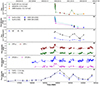 |
Fig. 1. Optical, UV, and X-ray light curves for the entire period of our monitoring. From top to bottom, we show (a) 0.2–5.0 keV flux from Swift-XRT, XMM-Newton-EPIC, and eROSITA, (b) UVM2- and UVW1-band flux densities from Swift-UVOT and XMM-Newton-OM, and (c) line fluxes for the broad Hβ and Hα emission components, integrated over the whole broad profile (Sect. 4.4.1). (d) ZTF g- and r-band, (e) ATLAS c- and o-band, (f) WISE W1 and W2 bands. In panels (a), (b), (d), and (e), there are some data points for which the error bars are smaller than the marker for the data point. |
3.2. SRG/eROSITA
eROSITA detected the object during each of its first four all-sky scans, eRASS1–4. We combined data from all seven telescope modules. We used event data from processing version c020 and the eROSITA data analysis software eSASS version eSASSuser 211214 (Brunner et al. 2022) in High Energy Astrophysics Software (HEASOFT) version 6.29. For each dataset, a circle and an annulus were used for the source and background regions, respectively. The radii were selected based on source brightness, where larger regions correspond to the source being brighter. The source region sizes varied between 105″ (most bright) and 47″ (least bright). Detected neighboring sources were excluded from the background regions in order to avoid background contamination. We list the eROSITA observations in Table 1.
X-ray and space-based optical/UV observations of J0428−00.
3.3. Swift
We observed J0428−00 12 times using the Neil Gehrels Swift Observatory (Swift;Gehrels et al. 2004). Ten pointings occurred during the initial flaring state between February and March 2020, the 11th observation occurred in December 2021, and the final observation occurred in March 2023.
The X-ray Telescope (XRT) exposures varied from 0.5 to 5.7 ks (Table 1). We calibrated the event files using xrtpipeline in HEASOFT version 6.29 and the latest calibration files. All spectra were extracted with circular regions of 40″ for the source and the background. We generated the ancillary response files using xrtmkarf, and the response matrix (RMF) was taken from the latest calibration database.
For the Ultraviolet/Optical Telescope (UVOT) data, we selected a circular region of 5″ for the source and a 25″ circular region located a few arcminutes from the source for the background for images taken by each of the UVOT filters. We used the task uvotsource to perform photometry and estimate fluxes for each of the available filters for the given observation. We applied Galactic extinction correction externally following the extinction estimates from Schlafly & Finkbeiner (2011). We also used the task uvot2pha to generate XSPEC-readable spectral files for the purpose of modeling simultaneous optical-UV-X-ray SEDs.
3.4. XMM-Newton
Two XMM-Newton (Jansen et al. 2001) observations (PI: M. Krumpe) with total durations of 38 ks and 55 ks were taken on 23 March 2022 and 14 March 2023, respectively (Table 1). The EPIC observations were taken in full-window mode. We reduced the EPIC-pn data with SAS v21.0.0 and HEASOFT v6.28 using standard procedures for point sources. A 40″ circular region centered around the source was used to extract the source spectrum. The background spectrum was extracted from a circular source-free region of the same radius, a few arcminutes away from the source. After high-background cleaning, 21.0 ks and 40.0 ks of good EPIC-pn integration time is left, corresponding to 0.2–10 keV spectral counts of 3.31 × 10³ and 5.34 × 10³, respectively. We found no evidence of pileup in either spectrum according to the XMMSAS task epatplot.
We reduced the Optical Monitor (OM) imaging-mode data using the omichain pipeline processing. This command applies flat fielding, source detection, and aperture photometry, and it ultimately creates mosaicked images. We used the om2pha command to generate XSPEC-readable spectral files for all the available filters (Table 1).
3.5. Optical spectroscopy
We obtained 11 long-slit spectra from January 2020 to March 2023 (referred to as spectra S1–S11), as summarized in Table 2. We obtained one spectrum at each of the following facilities: the 10 m class Keck telescope (Oke et al. 1995); the 5 m class Hale Telescope6; and the 1.9 m telescope (Crause et al. 2019) at the South African Astronomical Observatory (SAAO). We also obtained two spectra from the 8 m class Very Large Telescope (VLT, Appenzeller et al. 1998), a part of the European Southern Observatory (ESO). We also obtained three spectra each using the 4 m class Lowell Discovery Telescope (LDT)7 and the 10 m class Southern African Large Telescope (SALT; Buckley et al. 2006). All observations were made with the slit at parallactic angle. The spectral resolution of all our optical spectra ranged between 400 and 1300.
Optical spectroscopic observations of J0428−00 during 2020–2023.
The Keck spectrum was reduced using the LPipe package. The LDT and SALT spectra were reduced with standard IRAF routines. The VLT spectra were reduced using the EsoReflex package. The DBSP spectrum was reduced using the DBSP_DRP program.
For all spectra, corrections for atmospheric absorption were made following standard procedures. For example, for the SAAO spectrum, we applied corrections in the telluric A band (7588–7700 Å) and B band (6855–6965 Å). A correction for water vapor in the wavelength range 7150–7400 Å was also applied, although the impact was negligible. We used the spectral atmospheric transmission coefficients from the SMARTS2 atmospheric transmission model (Gueymard 2019, and references therein). Application to the spectrum removes the telluric A- and B-band absorption quite adequately, and the continuum looks smooth in the telluric absorption bands.
We performed flux scaling for each spectrum by fitting the [O III]λ5007 line profiles following the well-established framework of van Groningen & Wanders (1992). The method estimates a flux correction factor for the [O III]λ5007 line. It additionally corrects for wavelength-related calibration issues by cross-matching the central wavelength of the [O III] emission line (see Appendix A for details). A dereddening correction was also applied to all optical spectra before the spectral fitting using the Python package extinction8, where the value of E(B − V) was 0.064, obtained via the Python package sfdmap9 (Schlafly & Finkbeiner 2011).
4. Analysis and results
4.1. Optical continuum variability
All optical bands dramatically start to increase in flux starting around MJD 58855, and they increase for 30–35 days before they reach maximum flux around MJD 58885–58890. The factors of increase are 1.6, 1.3, and 1.2 for the ZTF g, ZTF r, and ATLAS o bands, respectively (ATLAS c band is relatively sparsely sampled), but these values do not account for host galaxy contamination. The optical fluxes then decay; we tracked the decrease for an additional 30 days before the Sun gap, which started around MJD 58920 for the g, r, and o bands. The factors of decrease are 1.4, 1.15, and 1.15 for g, r, and o, respectively, which is consistent with a time-symmetric flare.
We searched for any interband lags via cross correlations using the interpolated correlation function (ICF; Gaskell & Sparke 1986; Peterson et al. 1998). All four ATLAS and ZTF light curves are well correlated with each other (the maximum correlation coefficient rcorr is in the range 0.60–0.86), but there is no robust evidence for any lags or leads. The upper limits range from 4 to 26 days.
There is a broad flare in the two WISE light curves, with increase magnitudes in 0.4 (W1) and 0.6 (W2) that peak 0.5–1 year after the optical flare. The upper limit on any WISE W1 to W2 lag is 375 days. While ICFs comparing all four optical bands to W1 yielded only tentative lags or upper limits, all four optical light curves were found to lead the W2 band, with an average lag of 174 ± 114 d. A variable signal from the inner accretion flow (disk or corona) can yield a delayed reverberation signature from an extended dust structure in the IR bands. This delay would depend on the dust-sublimation radius of the system and on dust morphology relative to our line of sight. Assuming an average bolometric luminosity of 4 × 1043 erg s−1, an average dust-temperature of 1500 K and, an isotropic dust distribution, and using the estimate of dust submimation radius (Rsub) from Netzer 2015, we obtain Rsub = 0.1 parsec. This estimate corresponds to a light travel time of 120 days, which is consistent with the delay estimates of the W1 and W2 light curves with respect to the optical bands.
4.2. X-ray and ultraviolet continuum
We used the Bayesian X-ray analysis10 package (BXA, version 4.0.6, Buchner et al. 2014), implementing the nested sampling algorithm Ultranest (version 3.5.5 Buchner 2021) in XSPEC (version 12.12.0) to fit the X-ray data. The fit statistic was set to cstat. We froze the Galactic absorption NH to 5.77 × 1020 cm−2 (Willingale et al. 2013).
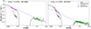 |
Fig. 3. Broadband SED fits for (a) the first Swift SED, taken near the flare peak in February 2020, and (b) the first XMM-Newton SED, taken in February 2022, assuming a black hole mass of MBH = 4 × 10⁸ M⊙. In each plot, the dashed blue line denotes the intrinsic unabsorbed AGN continuum. The dotted black line denotes the stellar contribution of the host galaxy. The solid black line denotes the Galaxy-absorbed total (AGN + host galaxy) model. The green markers represent the X-ray data and the magenta markers represent optical data. In each panel, the y-error bars are smaller for some data points than the data point marker. |
We fit a simple power-law model to all spectra, and acceptable fits were obtained in all cases. ΓX remains at relatively moderate values, and the average of the best-fitting values is 1.9 (Table 3) over the entire campaign, without any detected systematic variability (the scatter in the best-fitting values is 0.25, compared to the average of the errors of 0.4). We also tested for the presence of a soft X-ray excess (e.g. Turner & Pounds 1989) by adding a phenomenological blackbody component ZBBODY. No improvement was found for any spectrum, however11. The 0.5–1.0 keV ZBBODY flux was ≲10−4 of the total flux. We also tested for the presence of line-of-sight neutral obscuring gas, modeled with ZTBABS, but no improvements to the fits were obtained, with upper limits to the column density around 1020 cm−2. We thus conclude that the X-ray spectrum can be explained by a single unabsorbed power law (Fig. 2a) at all epochs.
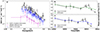 |
Fig. 2. X-ray spectra and light curves. Panel (a) shows the variation in the three selected X-ray spectra taken during the brightest phase, the minimum flux, and during the second peak. The round markers represent unfolded data and the solid lines represent best-fit model. Black represents the brightest X-ray observation from Swift, magenta represents the minimum flux observation from eROSITA and blue represents the second peak from Swift. Panels (b) and (c) shows the mean-normalized light curves exhibiting short-term variability in the decaying part of the flare, between MJD 58880 to 58920 for 0.2–5.0 keV X-ray and the UVW2 and UVM2 band, respectively. |
X-ray photon indices and model flux from power-law fits to all X-ray spectra.
Overall, the 0.2–5.0 keV X-ray continuum flux decays by a factor of 17 over two years. Minor short-term variability is superimposed on the decaying trend, as shown in Fig. 2b. All UV bands concurrently decay by roughly the same factor, and the X-ray and UV bands are all well correlated with each other at zero lag: The values of ICF correlation coefficients rcorr at zero lag are 0.884 (X-ray–UVW2), 0.915 (X-ray–UVM2), and 0.987 (UVW2–UVM2). The data sampling precludes any meaningful search for interband lags, however. The values of the fractional variability amplitude Fvar (Vaughan et al. 2003) for the X-ray, UVW2, and UVM2 light curves are 64.3 ± 5.9%, 40.5 ± 1.6%, and 50.0 ± 2.3%, respectively.
4.3. Broadband SED modeling
All Swift and XMM-Newton observations in our campaign were accompanied by simultaneous optical and UV photometry. We thus performed broad-band spectral fitting of all datasets. The broad-band spectral model contained a host galaxy template obtained from Mannucci et al. (2001), and the AGN broad-band spectral model was agnsed (Kubota & Done 2018).
Our model in XSPEC notation was redden*tbabs*(galaxy + agnsed). A comoving distance of 297 Mpc (Wright 2006), E(B − V) = 0.06412 (Schlafly & Finkbeiner 2011) and NH, Gal = 5.77 × 1020 cm−2 (Willingale et al. 2013) were assumed. We used a black hole mass of MBH = 4 × 10⁸ M⊙ (see Section 4.6). For all cases, we froze the value of the hard X-ray photon index (Γhot or ΓX) to the value obtained from the corresponding X-ray analysis. We kept the temperature of the hot corona (kBThot), the temperature of the warm corona (kBTwarm), and the corona height frozen to 100 keV, 0.1 keV, and 10 Rg respectively. The normalization of the host galaxy was kept frozen at the value obtained from the 2022 XMM-Newton observation. For all broad-band analyses, we performed GW-MCMC (Goodman & Weare 2010) fitting with a chain length of 10 000 and 20 walkers.
The values of the best-fitting parameters from our MCMC fitting and the errors corresponding to the 90% confidence range are reported in Table 4. We obtained acceptable fits, which indicates that in the context of the agnsed model, hot-Comptonization of seed photons from the accretion disk can adequately explain the X-ray spectrum of the source (Fig. 3) at all stages, with no requirement for significant soft-excess emission from a warm corona. The accretion rate relative to Eddington, λEdd ≡ LBol/LEdd, decreases by a factor of 8 across our observations, from log(λEdd) ≃ − 2.1 in February 2020 to ≃ − 3.0 in March 2023.
Parameters from broad SED fits assuming a black hole mass of 4 × 10⁸ M⊙.
4.4. Optical spectroscopic analysis
The evolution of the optical spectrum across our three-year campaign, along with the archival 6dF spectrum from 2005, is plotted in Fig. 4.
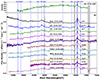 |
Fig. 4. Optical spectra of J0428−00. Panel (a) displays the 6dF spectrum from 2005 (not flux-calibrated), wherein no broad Hβ emission is detected above the continuum. Panel (b) shows the spectra taken during our 2020–2023 campaign. The spectra are not extinction corrected. The grey bands mark telluric absorption bands. |
4.4.1. Phenomenological emission line fitting
J0428−00 exhibits the narrow emission lines typically seen in Seyfert AGNs: the [O III]λλ4959,5007 doublet, the [N II]λλ6548,6584 doublet, and the [S II]λλ6716,6731 doublet (Fig. 4). Additionally, the source persistently exhibits a broad Hα emission line; as discussed below, broad Hβ is detected in all spectra except for the archival 6dF spectrum. Our spectral modeling is described below.
-
Local continuum. For all spectra, we fit the line region over a limited wavelength range by applying a local continuum to account for the continuum flux surrounding the wings of the emission line, following standard practices (e.g. Peterson et al. 1991). The local continuum for the Keck (S1) and all LDT spectra (S2–S4) is a host galaxy template plus a power law to model the AGN continuum. For all of the other seven (lower signal-to-noise ratio) spectra, it sufficed to adopt a model consisting of a host galaxy template plus a linear function; given the weakness of the latter component, it cannot be definitely ascribed to AGN emission. The host galaxy was modeled using the S0 template from Mannucci et al. (2001).
-
Narrow lines. To fully fit the [O III]λλ4959,5007 doublet, depending on the signal-to-noise, we required one (all spectra except the S1 Keck and the first S2 LDT spectra) or two (for S1 Keck and the first S2 LDT spectra) moderately broad (FWHM ∼ 1000 km s−1) and blueshifted components in addition to the core narrow lines (Fig. 5b); these broad components are likely the product of an outflowing wind in the narrow line region (NLR). We did not adopt an additional blue component for the [N II] emission line doublet superposed on the broad Hα to avoid overparameterization, as we already obtained optimum fits considering narrow line profiles alone. For the low signal-to-noise [S II] line, we found upon inspection some asymmetries toward the blue wavelengths in the doublets for only a few spectra (most prominent in S1 LDT and S2 LDT), but they are not persistent and did not exhibit a consistent trend in relation to the continuum. Furthermore, we did not observe this doublet in the best-quality Keck spectrum. We therfore did not adopt any additional components for [S II] in any spectra. The narrow Hβ emission line is extremely weak and can only be detected robustly in the Keck spectrum (S1). We also found a narrow line feature at λ ≃ 4893 Å in the Keck spectrum (S1) and the first two LDT spectra (S2–S3). This line feature is at a wavelength that is consistent with [Fe VII]λ4893. We caution that this identification is tentative, however, because a line like this typically does not appear in isolation and is accompanied by other coronal lines, such as [Fe VII] λ3759, 4893, 5159, 5276, 5720, and 6086 (Rose et al. 2011), which are not detected in J0428−00. All errors on the integrated narrow line fluxes were calculated with the least-squares fitting method.
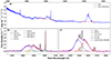
Fig. 5. Spectroscopic analysis of the extinction-corrected Keck spectrum. Panel (a) displays the local continuum fit. We fit the local continuum around the broad Hβ and broad Hα line regions using a power law plus host-galaxy template. Panel (b) shows the local continuum-subtracted Hβ line region. The best-fitting model consists of red- and blueshifted broad Gaussians to fit the broad Hβ emission profile, as well as Gaussian profiles fit to the narrow [O III]λλ4959,5007 doublet, including two blueshifted components for each line. The narrow gray Gaussian profile coincides with [Fe VII]λ4893 emission, but this identification is tentative (see text for details). Panel (c) shows the local continuum-subtracted Hα line region. The best-fitting model includes red- and blueshifted broad Gaussians to fit the broad Hα profile, as with Hβ. There are also narrow Gaussian profiles fit to the [N II]λλ6548,6584 and [S II]λλ6716,6731 doublets, as well as to narrow Hα.
-
Broad emission lines. Broad Hβ emission is detected in all of the 2020–2023 spectra; a model lacking broad Hβ is a worse fit, according to the Akaike information criterion (Akaike 1974). In the spectra with a relatively lower signal-to-noise (S5, S6, S8, and S10), a single broad Gaussian fit sufficed to describe the broad Hα profile, and a double Gaussian provided no additional fit improvement. For all other (higher signal-to-noise) spectra, a double-Gaussian model was necessary to achieve the best description of the profile, and consistent with J0428−00 as a double-peak emitter, as reported by Ward et al. (2024)13. The broad Hα line was fit well with a double-Gaussian profile. The parameter uncertainties for the broad components were estimated by the maximum likelihood method. The best fits to the Hβ and Hα profiles in the Keck spectrum (S1) are plotted in Fig. 5.
The model fit results are summarized in Tables B.1 and B.2. The best fit to the Keck spectrum (S1) is plotted in Fig. 5 to illustrate the profile decompositions.
The resulting light curves of broad Hβ and Hα fluxes of our campaign are plotted in the bottom panel of Fig. 1. The Hβ and Hα fluxes decay roughly in concert, with maximum-to-minimum flux ratio of 5.8 ± 0.2 for Hβ and 4.2 ± 0.2 for Hα. The values of the fractional variability amplitude Fvar are 60 ± 6% for Hβ and 41 ± 2% for Hα. The two broad Balmer fluxes correlate well with X-ray and UV continuum fluxes: zero-lag ICF values are 0.865 (X-ray–Hβ), 0.837 (UVW2–Hβ), 0.859 (UVM2–Hβ), 0.835 (X-ray–Hα), 0.701 (UVW2–Hα), and 0.722 (UVM2–Hα). Again, the data sampling precludes any meaningful search for lags or leads, however.
We also modeled the broad Balmer profiles in the archival 6dF spectrum from 2005. Broad Hα emission was detected, and a double-Gaussian model provided a superior fit to a single-Gaussian model. No broad Hβ emission is detected, however. The addition of a single- or double-Gaussian model yielded no improvement to the fit. The spectral decomposition is displayed in Fig. B.1. Our analysis supports the source classification as a type 1.9 in the 6dF spectrum14 and supports that the source underwent an optical spectral type change from 2005 to 2020 (Frederick et al. 2020). The 6dF spectrum is not flux calibrated, however, and a direct comparison of the flux estimates with the recently obtained spectra is therefore not possible.
To further quantify the evolution in the Hβ profile across all spectra, including 6dF, we considered the ratio of broad Hβ flux to the sum of the fluxes in the [O III] λ5007 profile, as defined by Winkler (1992): RHβ/[O III] ≡ F(Hβ)/F([O III]). In Fig. 6 we plot the resulting values of RHβ/[O III] as a function of time for the 2020–2023 spectra. Because no broad Hβ emission is detected in the 6dF spectrum, the resulting upper limit on RHβ/[O III] is ∼1.0, which is plotted as the dashed red line. RHβ/[O III] jumped from < 1.0 in 2005 to values near 5–6 in early 2020, and it then faded to values between 1.0 and 2.8 for the remainder of thecampaign.
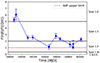 |
Fig. 6. Ratio of the broad Hβ flux to narrow [O III] λ5007 flux, RHβ/[O III], as a function of time for the 2020–2023 spectra. The ratio is plotted using the round blue marker. The dashed blue line represents the approximate trend. The upper limit to RHβ/[O III] from the archival 6dF spectrum is plotted as the dashed red line. The solid horizontal lines denote the boundaries between Seyfert subtypes following Winkler (1992). |
We also used RHβ/[O III] to assign approximate Seyfert subtypes to all spectra, and we tracked the subtype evolution of J0428−00. Following Winkler (1992), subtypes 1.0, 1.2, 1.5, and 1.8 correspond to RHβ/[O III] > 5, 2 < RHβ/[O III] < 5, 0.33 < RHβ/[O III] < 2, and RHβ/[O III] < 0.33, respectively. These regimes are marked in Fig. 6. We classified the 6dF spectrum as subtype 1.9 because no broad Hβ is detected, while Hα clearly is detected. The early 2020 spectra, Keck (S1) and the first LDT spectrum (S2) are subtype 1.0. The other nine spectra, from late 2020 through 2023, are all subtypes 1.2–1.5. We note two caveats regarding the use of RHβ/[O III] as a generic quantity for subtype classification, however, which can introduce mild uncertainties in the precise subtyping. With regard to comparing different objects and/or when different instruments are used, (a) intrinsically, different objects will span different ranges of NLR characteristics and host galaxy star formation activity. (b) The differences in configuration (e.g., aperture) from one instrument to the next can lead to different measurements of [O III], host galaxy light, and so on. Nevertheless, for J0428−00, the evolution in its subtype classification reinforces the significant evolution in the relative line strengths we observed. This is consistent with its status as a changing-lookAGN.
4.4.2. Testing the physical diskline model
For the best-quality spectrum, which is the spectrum taken with Keck, we tested whether a physically motivated double-peaked profile from a disk emitter (Chen et al. 1989; Chen & Halpern 1989) explains the observed Hα and Hβ profiles. This model (henceforth “diskline”) assumes that the line-emitting matter is in Keplerian motion in a flattened geometry, and it incorporates the effects of Doppler shifts and gravitational redshift. Following Chen & Halpern (1989), we applied local broadening due to electron scattering in a photoionized atmosphere (Halpern 1984; Shields & McKee 1981). The emissivity profile assumes isotropic illumination from the center.
Best-fitting parameters from diskline fits to the broad Balmer profiles in the Keck spectrum.
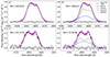 |
Fig. 7. Diskline model fits to the broad Hα and Hβ emission line profiles – narrow line and continuum subtracted – as described in Section 4.4.2. Hα profile is fit with (a) single diskline and (b) combination of diskline and a Gaussian profile. Hβ profile is fit with (c) single diskline and (d) combination of diskline and a Gaussian profile, with best-fitting parameters independent of those for the Hα profile fit. The dashed line represents the zero flux density level. |
We isolated the broad emission lines by subtracting the underlying continuum and best-fit narrow profiles obtained from the phenomenological Gaussian fitting (Section 4.4.1). We tested a model with only a diskline component (A) and a model with a diskline plus a broad Gaussian component (B). For both Hα and Hβ, the Akaike information criterion indicates a strong preference for model B: The addition of the broad Gaussian caused the value of AIC to drop by over 15 and improved the data-model residuals, as plotted in Fig. 7. The center of the broad Gaussian was consistent with a zero-velocity offset.
We list the best-fitting model parameters for model B in Table 5. The best-fitting geometrical parameters from Hα are consistent with those obtained for multiple double-peaked emitters by Ward et al. (2024) using a similar diskline model. For all fits, we obtained a consistent inclination, θi ≃ 15°. Overall, our analysis indicates that the Hβ and Hα emission lines contain similar emissioncomponents.
4.5. Diagnostics of historical AGN activity
We diagnosed the historical AGN activity in J0428−00 via Baldwin, Phillips, and Terlevich (BPT) diagrams (Baldwin et al. 1981) using the best-fitting Gaussian parameters to the narrow lines. We plot the flux ratios for both [O III]λ5007/Hβ versus [N II]λ6584/Hα and [O III]λ5007/Hβ versus [S II]λ6717/Hα along with classification curves from Schawinski et al. (2007), Kewley et al. (2001), and Kauffmann et al. (2003) in Fig. 8. In all spectra except the Keck spectrum, the narrow Hβ line had a low signal-to-noise ratio, and its flux was not constrained. We therefore adopted the narrow Hβ line flux from the Keck spectrum for all spectra. For most of the observations, the [O III]λ5007/Hβ line flux ratio is high enough to position the object in the AGN region of the BPT diagram (the region above the solid blue curve in Fig. 8). This indicates that the nucleus of J0428−00 has been in a prolonged (∼103 − 104 years) persistently accreting state.
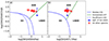 |
Fig. 8. BPT diagrams (Baldwin et al. 1981) to assess the activity in J0428−00. The line ratios (panel a) [N II]λ6583/Hα and (panel b) [S II]λ6717/Hα are plotted against the line ratio [O III]λ5007/Hβ. The classification curves are taken from Kewley et al. (2001), Kauffmann et al. (2003), and Schawinski et al. (2007). |
4.6. Estimating the black hole mass and Eddington ratio
We estimated the black hole mass by using standard empirical relations between MBH, FWHM velocity, and λL5100, calibrated against nearby Seyferts whose black hole masses were measured via BLR reverberation mapping. For J0428−00, we used the best signal-to-noise spectrum from Keck to estimate the above quantities. For the Keck spectrum, the best-fitting FWHM velocity of Hβ is 8140 km s−1 and λL5100 = 4.62 × 1043 erg s−1. We used Eq. (4) from from Vestergaard & Peterson (2006) for the Hβ broad line, and we obtained the estimate  .
.
We also used the radius-luminosity relation between λL5100 and BLR radius (RBLR) along with the Hβ FWHM to estimate the black hole mass using the scaling relation from Bentz et al. (2009):  . We used the average inclination obtained from the diskline fits (15.7°) to calculate the virial factor following Mejía-Restrepo et al. (2018)
![Mathematical equation: $$ \begin{aligned} f_{\rm vir} = [4 ( \sin ^2(i) + (H/R)^2)]^{-1}. \end{aligned} $$](/articles/aa/full_html/2025/10/aa47985-23/aa47985-23-eq45.gif) (1)
(1)
For the assumed values of the aspect ratio H/R spanning 0.01–0.10, we obtained values of fvir that spanned 3.2–3.7. Mejía-Restrepo et al. (2018) and Yu et al. (2019) also indicated that the virial factor is inversely proportional to the FWHM of the line, however, and that it might be as low as 0.5 for FWHM values as high as 8000 km s−1. For values of fvir = 0.5 or 3.7, we therefore obtained black hole masses of  and
and  , respectively. We adopted the average of all these estimates, 4 × 10⁸ M⊙, for all calculations. As a caveat, however, the standard relations used below are based on persistently accreting Seyferts, while J0428−00 was monitored while undergoing a sudden transient luminosity flare.
5. Discussion
5.1. Summary of the main observations
The source exhibited a sharp flare in the optical continuum in early 2020, with a flux increase over 35 days that was followed by a decay that we were able to track for an additional ∼30 days before the Sun gap. The optical spectrum meanwhile underwent a transition: In the 2005 spectrum, no broad Hβ emission was detected (subtype 1.9). In the spectra taken during January–February 2020, broad Hβ emission was present and strong (Fig. 4), consistent with subtype 1.0 (Sect. 4.4.1). The profiles of broad Hα and Hβ are fit well by a double-peaked profile. After the flare peak in the optical, we tracked the subsequent decay in the optical, UV, and X-ray continua until 2023. The broad Hα and Hβ emission line fluxes track the long-term continuum (Fig. 1).
The X-ray spectra are fit well by a single unabsorbed power law with a flat photon index (∼1.9). The X-ray and UV continua decay in concert, and the broadband SED (Fig. 3) is consistent with the X-rays being generated by thermal Comptonization of low-energy seed photons from the accretion disk. Intriguingly, soft X-ray excess, a near-ubiquitous feature of the X-ray spectra of nearby Seyferts, is absent in J0428−00.
J0428−00 exhibits persistent narrow emission lines of [O III]λλ4959,5007, [N II]λλ6548,6584, and [S II]λλ6716,6731. The resulting BPT-diagnostic ratios (Fig. 8) indicate ongoing AGN activity for some millennia.
Finally, the WISE IR light curves exhibit a broad flare (Fig. 1), with the peak in W2 delayed by roughly 170 days with respect to the main optical flare. This is consistent with a dust echo in circumnuclear warm dust.
We construct the large picture of the connection of the temporary continuum flaring to the optical spectral changing-look transition, the X-ray emission, and the IR flux peak. We speculate on the underlying mechanism(s) that causes the flare.
5.2. Characteristics of the transient
The nature of a supermassive black hole transient flaring event can be consistent with either AGN-like accretion or with a tidal disruption event (TDE) of a star by a quiescent black hole (Rees 1988; Evans & Kochanek 1989). While TDEs can occur in quiescent galaxies, recent observations have uncovered some nuclear transients that display attributes consistent with both TDE- and AGN-like accretion, suggesting that the two channels of accretion can occur simultaneously (e.g., Ricci et al. 2020; Holoien et al. 2022; Homan et al. 2023).
The X-ray spectra of J0428−00 are Seyfert-like. Their photon index ΓX remains near 1.9, and we observe no drastic variation in the photon index. This hard X-ray spectral behavior (Auchettl et al. 2018) is inconsistent with that demonstrated by thermal TDEs, which typically exhibit much softer X-ray spectra (ΓX > 3, typically; e.g., Gezari 2021). As a caveat, however, the hard X-ray photon index distribution of TDEs is broad and can sometimes encompass such low values (e.g., with ∼0.3 probability as per Auchettl et al. 2018).
Other observations in J0428−00 instead support AGN-like accretion: A persistent broad Hα line was seen in the archival 6dF spectra and during the recent campaign. This is indicative of AGN activity in 2005 and during 2020–2023. This is also supported by the narrow-line BPT diagnostics (Figure 8), which classify this source as an AGN with a prolonged accretion activity.
The ratio of the luminosity of the hard X-ray luminosity to the luminosity of the [O III]λ5007 line can also distinguish between persistent AGN activity over the last ∼103 − 104 years versus a TDE event (Heckman et al. 2005). Sazonov et al. (2021) found this ratio to be around 102 in a sample of local AGNs and around 104 in a sample of TDEs. For J0428−00, we estimated the ratio RX/[O III] of L0.2−6.0 keV/L[O III] following Sazonov et al. (2021). At flare peak, when the X-ray luminosity highest, RX/[O III] is 102.8. Three years after the peak passed, RX/[O III] was 102.0. The high value of RX/[O III] near the flare peak can be interpreted as being due to a rapid but temporary increase in the X-ray flux during the outburst, while the [O III]λ5007 line flux remained static.
To summarize, the observed activity in J0428−00 appears to be more reminiscent of a temporary change in the accretion rate in a disk-like accretion flow in a persistently accreting AGN than accretion from a tidally disrupted star. We consider the emission and variability properties in the context of AGN accretion below.
5.3. Origin of the X-ray continuum
As noted above, the X-ray photon index ΓX stayed near roughly 1.9 as the multiband continuum flaring decayed (Section 4.2 and Table 3). This value is consistent with hot-Comptonization of seed photons from an accretion disk in a hot corona (Haardt & Maraschi 1991, 1993) in Seyfert galaxies (e.g., Mateos et al. 2010). We found no evidence for significant X-ray spectral variability over three years despite the strong X-ray continuum flux variability. In principle, ΓX is dependent on the ratio of heating (e.g., from magnetic processes; Balbus & Hawley 1998) to cooling (from upscattering of seed photons) in the corona (Eq. (14) in Beloborodov 1999). It is conceivable that in J0428−00, (a) the total energy injected into the corona by the incident seed remained lower than the total internal energy of the corona during the continuum decay, and/or (b) coronal parameters such as optical depth or geometry remained stable over time, and flux variations in the X-rays resulted from seed photon variations, but without coronal cooling.
Changing-look AGNs display a wide range of X-ray variability properties across multiple sources. For example, NGC 1566 exhibited an outburst in which the spectral evolution resembled a q-diagram in the hardness-intensity plane (Jana et al. 2021). Its X-ray photon index was qualitatively consistent with the ΓX–flux relations observed in normal Seyferts and black hole X-ray binaries (BHXRBs) (e.g. Papadakis et al. 2009) and hardness intensity characteristics of BHXRBs (e.g. Remillard & McClintock 2006). In contrast, two X-ray spectra taken two years apart in the CLAGN IRAS 23226−3843 (Kollatschny et al. 2023) only varied in the X-ray normalization following an outburst, without significant evolution in the X-ray spectral shape. This behavior is qualitatively similar to that seen following the flare in J0428−00.
A soft X-ray excess, manifested as a very steep power-law-like emission below roughly 1–2 keV, is near-ubiquitous in normal Seyferts (Halpern 1984; Turner & Pounds 1989). The absence of a soft excess in the X-ray spectra of J0428−00 is puzzling. Its origin in normal Seyferts is debated (e.g., Sobolewska & Done 2007). The leading models are thermal Comptonization from a warm (kBTe ∼ 1 keV) optically thick (τ ≳ 10) corona (Mehdipour et al. 2011; Done et al. 2012; Petrucci et al. 2018) or blurred reflected emission from the innermost ionized accretion disk (Crummy et al. 2006; García et al. 2013). In the first case, the lack of an observed soft excess above 0.2 keV might mean that a warm corona is simply physically absent in J0428−00. Alternately, our broadband SED fits (Section 4.3) using AGNSED suggest that if a warm corona is present, its emission remains localized to energies below 0.2 keV, while all emission above 0.2 keV is Comptonization from the a hot corona. Given the range of accretion rates for J0428−00 inferred during our campaign, log(λEdd) ∼ –2 to –3, the lack of soft excess is consistent with the findings of Hagen et al. (2024), that the soft excess is typically absent in the X-ray spectra of sources that accrete at values of log(λEdd) below roughly –1.5. In the case of blurred reflection, on the other hand, this component might be absent because there is no optically thick cold accretion disk in the innermost regions of the accretion flow. This leads to inefficient illumination by and reflection of the X-ray continuum photons. A final possibility is that this disk component exists, but is overionized.
5.4. The stability of the accretion structure
Major changes in the overall disk and corona structure in AGNs or quasars can be tracked via the UV-to-X-ray spectra index αOX (Tananbaum et al. 1979). Evolution in αOX as a function of λEdd has been recorded both in samples of normally varying quasars (e.g., Lusso et al. 2010) and in individual changing-look quasars (Ruan et al. 2019). For J0428−00, we obtained the values from the SED fits in Sect. 4.3. The resulting values of αOX during our campaign span from from 1.1 to 1.4, averaging near 1.2. The scatter in αOX is due to the short-term variability in the UV and especially the X-ray bands, but αOX exhibits no systematic trends that would preclude major changes in the global disk/corona structure. These values of αOX are similar to those for X-ray-selected type-1 quasars at the same UV luminosity, as reported by Lusso et al. (2010).
5.5. Broad Balmer lines and emitter geometry
The broad Hα emission line is persistent in all stages of observation, including in 2005, whereas the broad Hβ only appeared during the 2020–2023 transient event and varied much more strongly than the Hα line (Fig. 1f). Wu et al. (2023) demonstrated that major changes in the Balmer decrement can be driven by changes in the incident ionization continuum due to a change in accretion rate. This change in the ionizing flux affects the responsivity of the Hβ emission line more than the Hα line due to the Q-dependent opacity in the emitter (details are given in Section 5 of Wu et al. 2023). This might lead to large relative changes in the broad Hβ line strength in intermediate-type Seyferts, which might trigger a CLAGN transition. In Fig. 9 we plot the Balmer decrement as a function of λEdd for our 2020–2023 optical spectra. For each optical spectrum, we estimated λEdd based on the X-ray flux from the X-ray observations nearest in time, and we used the bolometric corrections from Duras et al. (2020). As the continuum flaring fades, the Balmer decrement increases substantially (factor of 2.2); this behavior is qualitatively consistent with the theoretical predictions of Wu et al. (2023), as well as with the empirical behavior of the Seyferts and CLAGN discussed therein.
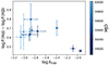 |
Fig. 9. Balmer decrement as a function of the accretion rate relative to Eddington for our 2020–2023 optical spectra. The markers indicate the values and the shades on the markers indicate time: a deeper shade indicates an earlier time as shown by the colorbar. |
Furthermore, the optical broad lines are double peaked. The broad line profiles of the high signal-to-noise Keck spectrum can explained by a diskline component that extends from around 500 Rg to 1000 Rg, consistent with Ward et al. (2024). It is a general trend that double-peaked Balmer line profiles are found prevalently in low-luminosity AGNs (Elitzur & Ho 2009; Elitzur et al. 2014). Similar trends are predicted by the dynamic failed radiatively accelerated dusty outflow (FRADO, Naddaf et al. 2021; Naddaf & Czerny 2022) for values of the Eddington ratio (λEdd) below roughly 10−2. J0428−00 broadly exhibits an Eddington ratio < 10−2 near its peak, and the observed profile of its broad emission lines is thus consistent with the trends described above.
5.6. A possible origin for the flare
Constraints on the mechanism driving the luminosity flare can be derived from comparing the observed flaring timescale (≳1 month) to standard timescales of variability associated with a accreting disk of matter (e.g. Treves et al. 1988). The standard timescales for AGN variability are the light-crossing (tlc = R/c), dynamic ( ), thermal (tth = (1/α)tdyn), and viscous (tvisc = (H/R)−2tth) timescales, where α and H are the viscosity parameter and the disk thickness respectively. At arbitrary radii of R ∼ 10 − 100 Rg, assuming a viscosity parameter α of 0.1, a scale height H/R of 10−3 (for a thin disk) and 1 (for a thick disk), and a black hole mass of MBH = 4 × 10⁸ M⊙, we find that the observed flare (roughly 35-day increase) is most compatible with the dynamical and thermal timescales, and the viscous timescale for a geometrically thick disk.
We posit that the flare in J0428−00 is compatible with, among other models, radiation pressure-driven disk instability models as described by Lightman & Eardley (1974) and Śniegowska et al. (2020), for example. In this model, an unstable annular region of the disk exists between a radiatively inefficient inner region and the geometrically thin outer disk. Initially, it is filled with tenuous gas, and new gas accretes inward from the outer disk on the viscous timescale for a thin disk; the luminosity increases only gradually. Initially, the gas pressure exceeds the radiation pressure. When the radiation pressure exceeds gas pressure locally, however, it triggers a heat wave that propagates inward on the local thermal timescale. It causes  to increase, and the shortened viscous timescale drives the local accretion rate to a drastic increase, leading to a burst of thermally emitted radiation. The unstable zone accretes its gas inward faster than gas is replenished. As cooling becomes greater than heating, the local accretion rate and luminosity subsequently fade; the cooling is dominated by the thermal timescale. The rise and decay times of the flare in the optical band (roughly a month) are each broadly consistent with the thermal timescale, a radiation pressure-driven instability therefore is a plausible explanation for the observed flaring in J0428−00.
Finally, we note that the light curves calculated from the simulations of Śniegowska et al. (2020, 2023) qualitatively resemble the observed light curves in J0428−00 in this manner.
6. Conclusions
We reported the detection of a new optical changing-look Seyfert: J0428−00 was originally a type-1.9 Seyfert, but it exhibited a multiwavelength flare in 2020 that was captured in the optical by ZTF and in the X-ray by eROSITA eRASS surveys. A change in optical spectral classification from type 1.9 to 1 was tied to the extreme variability, as broad Hβ emission had appeared by 2020. We initiated a three-year multiwavelength follow-up campaign to track the source emission as the flare gradually subsided and to determine the nature of this transient event.
The recent X-ray spectra, combined with indications of historical AGN activity, argue against the event being due to the tidal disruption of a star by a supermassive black hole. Instead, the flare is more likely the result of a disk instability in a previously existing accretion structure. Our additional key findings are listed below.
-
J0428−00 exhibits narrow emission lines of [O III]λλ4959,5007, [N II]λλ6548,6584, and [S II]λλ6716,6731. The BPT ratios indicate ongoing AGN activity for some millennia (Section 4.5).
-
J0428−00 exhibits double-peaked broad Balmer emission lines. Hα is relatively strong and persistent, even in the archival 6dF spectrum. Hβ only appeared in 2020, with RHβ/[O III] jumping from < 1.0 to 5–6. This is consistent with being driven by the continuum flare and the sudden increase in the flux of ionizing photons. The broad Balmer line fluxes overall track the continuum, and they fade slowly as the continuum flux subsides. The evolution in the Balmer decrement (Fig. 9) is qualitatively consistent with the expected response to the decay in the ionizing continuum (Wu et al. 2023). The double peaks of the broad Balmer profiles are fit well by models based on a disk-type geometry that extends from roughly a few hundred Rg to roughly 1000 Rg.
-
The X-ray spectra are fit well by a power law with a flat photon index (∼1.9), typical for radio-quiet Seyferts. In addition, the X-ray and UV continuua decay in concert (Fig. 1a and b). The X-rays are thus consistent with thermal Comptonization of low-energy seed photons. The relative stability in the photon index despite the strong X-ray variability might indicate a relative stability in the hot corona properties (τ; geometry), however.
-
Intriguingly, the soft X-ray excess, a near-ubiquitous feature of the X-ray spectra of nearby Seyferts, is absent in J0428−00. This might indicate the absence or extreme weakness of a warm corona in the context of warm Comptonization models (Section 4.3). The lack of the soft excess is consistent with the notion that the soft excess is typically missing in sources that accrete at values of log(λEdd) below roughly −1.5 (Hagen et al. 2024).
-
The WISE light curves exhibit a broad flare, with the peak in the W2 band delayed by roughly 170 days with respect to the main optical flare. This is consistent with reprocessing in a parsec-scale circumnuclear dust structure.
All these observations are consistent with a scenario in which the main trigger of the events is a temporary instability in the accretion flow structure. A Lightman-Eardley instability triggered in the inner disk (∼50 to 100 Rg) is consistent with the observed timescale of the main flare from 2020. Additionally, the continuum variability light curves of J0428−00 qualitatively resemble those that were theoretically calculated by Śniegowska et al. (2020) and Śniegowska et al. (2023). To summarize, this disk instability resulted in a temporary increase in the local accretion rate in the disk and yielded optical and UV thermal continuum flaring. In turn, the resulting increase in the optical and UV seed photons drove the observed X-ray flaring via thermal Comptonization, and the increase in ionizing the far-UV luminosity drove the increase in the broad Hβ flux as the preexisting disk-like BLR was illuminated. The optical, UV, and X-ray flaring emission later reached the dusty torus, which resulted in the observed IR flare.
Time-domain astronomy yields an ever-increasing accumulation of peculiar supermassive black hole transient events. The discovery of flaring activity in J0428−00 is part of this multiwavelength time-domain effort, and ot includes the new window of eROSITA into X-ray time-domain studies. CLAGN and flaring AGN are events that yield insight into major changes in the accretion rate, but these changes are sometimes temporary. Consequently, it is critical to study these events and understand the mechanism(s) that drives them to fully understand the accumulated accretion histories of AGN.
We consider subtypes 1.0, 1.2, 1.5, 1.8, and 1.9 to be subtypes of type 1 because the broad Hα line is present in all these cases. We follow Osterbrock (1981), Winkler (1992), and Runco et al. (2016), for example, in defining type 1.9 as having a broad Hα line that is detectable against the local continuum while the broad Hβ line is not detectable, and type 1.8 in having a broad Hβ line that is detectable, but weak. In all types 1.0, 1.2, 1.5, and 1.8, the strength of broad Hβ flux relative to the [O III] flux (Winkler 1992) or narrow Hβ flux (e.g., Osterbrock 1977, 1981), for example, decreases gradually.
The values of the Bayes factor BF were lower than one; BF ≡ Z2/Z1, where Z1 and Z2 denote the Bayesian evidence values for the simple power-law model and the alternative model, respectively.
Given the varying levels of signal-to-noise across our spectra, we do not claim that the broad Hβ line intrinsically changes profile between the single- or double-Gaussian shapes; it is simply a matter of preferring the simpler model when it provides an adequate fit.
Our analysis contradicts the claimed detection of Hβ by Chen et al. (2022) in the 6dF spectrum. In addition, the implied Balmer decrement value obtained by Chen et al. (2022) for the 6dF spectrum, with Hα flux being roughly one-third that of Hβ, is not physically feasible in AGN.
Acknowledgments
The authors thank the anonymous referee for the comments and suggestions. The authors acknowledge insightful discussions with Prof. Chris Done, Prof. Jiří Svoboda, and Prof. Piotr Życki. TS acknowledges full and partial support from Polish Narodowym Centrum Nauki grants 2018/31/G/ST9/03224 and 2016/23/B/ST9/03123, and partial support from Deutsches Zentrum für Luft- und Raumfahrt (DLR) grant FKZ 50 OR 2004. AM acknowledges full or partial support from Polish Narodowym Centrum Nauki grants 2016/23/B/ST9/03123, 2018/31/G/ST9/03224, and 2019/35/B/ST9/03944. DH acknowledges support from DLR grant FKZ 50 OR 2003. MK is supported DLR grant FKZ 50 OR 2307. MG is supported by the EU Horizon 2020 research and innovation programme under grant agreement No 101004719. SH is supported by the German Science Foundation (DFG grant number WI 1860/14-1). DAHB & JB acknowledge support from the National Research Foundation. This work is based on data from eROSITA, the soft X-ray instrument aboard SRG, a joint Russian-German science mission supported by the Russian Space Agency (Roskosmos), in the interests of the Russian Academy of Sciences represented by its Space Research Institute (IKI), and the Deutsches Zentrum für Luft- und Raumfahrt (DLR). The SRG spacecraft was built by Lavochkin Association (NPOL) and its subcontractors, and is operated by NPOL with support from the Max Planck Institute for Extraterrestrial Physics (MPE). The development and construction of the eROSITA X-ray instrument was led by MPE, with contributions from the Dr. Karl Remeis Observatory Bamberg & ECAP (FAU Erlangen-Nuernberg), the University of Hamburg Observatory, the Leibniz Institute for Astrophysics Potsdam (AIP), and the Institute for Astronomy and Astrophysics of the University of Tübingen, with the support of DLR and the Max Planck Society. The Argelander Institute for Astronomy of the University of Bonn and the Ludwig Maximilians Universität Munich also participated in the science preparation for eROSITA. The eROSITA data shown here were processed using the eSASS software system developed by the German eROSITA consortium. This work is based on observations obtained with XMM-Newton, an ESA science mission with instruments and contributions directly funded by ESA Member States and NASA. This research has made use of data and software provided by the High Energy Astrophysics Science Archive Research Center (HEASARC), which is a service of the Astrophysics Science Division at NASA/GSFC. This work has made use of data from the Asteroid Terrestrial-impact Last Alert System (ATLAS) project. The ATLAS project is primarily funded to search for near earth asteroids through NASA grants NN12AR55G, 80NSSC18K0284, and 80NSSC18K1575; byproducts of the NEO search include images and catalogs from the survey area. This work was partially funded by Kepler/K2 grant J1944/80NSSC19K0112 and HST GO-15889, and STFC grants ST/T000198/1 and ST/S006109/1. The ATLAS science products have been made possible through the contributions of the University of Hawaii Institute for Astronomy, the Queen’s University Belfast, the Space Telescope Science Institute, the South African Astronomical Observatory, and The Millennium Institute of Astrophysics (MAS), Chile. Based on observations obtained with the Samuel Oschin Telescope 48-inch and the 60-inch Telescope at the Palomar Observatory as part of the Zwicky Transient Facility project. ZTF is supported by the National Science Foundation under Grant No. AST-1440341 and AST-2034437 and a collaboration including Caltech, IPAC, the Weizmann Institute for Science, the Oskar Klein Center at Stockholm University, the University of Maryland, the University of Washington, Deutsches Elektronen-Synchrotron and Humboldt University, Los Alamos National Laboratories, the TANGO Consortium of Taiwan, the University of Wisconsin at Milwaukee, Trinity College Dublin, Lawrence Berkeley National Laboratories, Lawrence Livermore National Laboratories, and IN2P3, France. Operations are conducted by COO, IPAC, and UW. This paper uses observations made from the South African Astronomical Observatory (SAAO). Some of the observations reported in this paper were obtained with the Southern African Large Telescope (SALT) under programs 2020-2-MLT-008 (PI: A. Markowitz) and 2021-2-LSP-001 (PI: D. Buckley). Polish participation in SALT is funded by grant No. MEiN nr 2021/WK/01. The paper is based on observations collected at the European Southern Observatory under ESO programme 109.23MH.001. This publication makes use of data products from the Wide-field Infrared Survey Explorer, which is a joint project of the University of California, Los Angeles, and the Jet Propulsion Laboratory/California Institute of Technology, funded by the National Aeronautics and Space Administration. This publication also makes use of data products from NEOWISE, which is a project of the Jet Propulsion Laboratory/California Institute of Technology, funded by the Planetary Science Division of the National Aeronautics and Space Administration. This research has made use of the NASA/IPAC Extragalactic Database (NED), which is funded by the National Aeronautics and Space Administration and operated by the California Institute of Technology. We made extensive use of the following open-source python packages: NumPy (Harris et al. 2020), Matplotlib (Hunter 2007), SciPy (Virtanen et al. 2020), and Astropy (Astropy Collaboration 2022).
References
- Akaike, H. 1974, IEEE Trans. Automat. Control, 19, 716 [Google Scholar]
- Appenzeller, I., Fricke, K., Fürtig, W., et al. 1998, Messenger, 94, 1 [Google Scholar]
- Astropy Collaboration (Price-Whelan, A. M., et al.) 2022, ApJ, 935, 167 [NASA ADS] [CrossRef] [Google Scholar]
- Auchettl, K., Ramirez-Ruiz, E., & Guillochon, J. 2018, ApJ, 852, 37 [NASA ADS] [CrossRef] [Google Scholar]
- Balbus, S. A., & Hawley, J. F. 1991, ApJ, 376, 214 [Google Scholar]
- Balbus, S. A., & Hawley, J. F. 1998, Rev. Mod. Phys., 70, 1 [Google Scholar]
- Baldwin, J. A., Phillips, M. M., & Terlevich, R. 1981, PASP, 93, 5 [Google Scholar]
- Bellm, E. C., Kulkarni, S. R., Graham, M. J., et al. 2019, PASP, 131, 018002 [Google Scholar]
- Beloborodov, A. M. 1999, in High Energy Processes in Accreting Black Holes, eds. J. Poutanen, & R. Svensson, ASP Conf. Ser., 161, 295 [Google Scholar]
- Bentz, M. C., Peterson, B. M., Netzer, H., Pogge, R. W., & Vestergaard, M. 2009, ApJ, 697, 160 [Google Scholar]
- Brunner, H., Liu, T., Lamer, G., et al. 2022, A&A, 661, A1 [NASA ADS] [CrossRef] [EDP Sciences] [Google Scholar]
- Buchner, J. 2021, J. Open Source Softw., 6, 3001 [CrossRef] [Google Scholar]
- Buchner, J., Georgakakis, A., Nandra, K., et al. 2014, A&A, 564, A125 [NASA ADS] [CrossRef] [EDP Sciences] [Google Scholar]
- Buckley, D. A. H., Swart, G. P., & Meiring, J. G. 2006, in Ground-based and Airborne Telescopes, ed. L. M. Stepp, SPIE Conf. Ser., 6267, 62670Z [NASA ADS] [CrossRef] [Google Scholar]
- Chen, K., & Halpern, J. P. 1989, ApJ, 344, 115 [NASA ADS] [CrossRef] [Google Scholar]
- Chen, K., Halpern, J. P., & Filippenko, A. V. 1989, ApJ, 339, 742 [NASA ADS] [CrossRef] [Google Scholar]
- Chen, Y.-P., Zaw, I., Farrar, G. R., & Elgamal, S. 2022, ApJS, 258, 29 [Google Scholar]
- Crause, L. A., Gilbank, D., Gend, C. V., et al. 2019, J. Astron. Telesc. Instrum. Syst., 5, 024007 [CrossRef] [Google Scholar]
- Crummy, J., Fabian, A. C., Gallo, L., & Ross, R. R. 2006, MNRAS, 365, 1067 [Google Scholar]
- Denney, K. D., De Rosa, G., Croxall, K., et al. 2014, ApJ, 796, 134 [Google Scholar]
- Done, C., Davis, S. W., Jin, C., Blaes, O., & Ward, M. 2012, MNRAS, 420, 1848 [Google Scholar]
- Duras, F., Bongiorno, A., Ricci, F., et al. 2020, A&A, 636, A73 [NASA ADS] [CrossRef] [EDP Sciences] [Google Scholar]
- Elitzur, M., & Ho, L. C. 2009, ApJ, 701, L91 [Google Scholar]
- Elitzur, M., Ho, L. C., & Trump, J. R. 2014, MNRAS, 438, 3340 [Google Scholar]
- Evans, C. R., & Kochanek, C. S. 1989, ApJ, 346, L13 [Google Scholar]
- Fausnaugh, M. M. 2017, PASP, 129, 024007 [NASA ADS] [CrossRef] [Google Scholar]
- Frederick, S., Graham, M. J., Gezari, S., van Velzen, S., & Ward, C. 2020, ATel, 13460, 1 [Google Scholar]
- García, J., Dauser, T., Reynolds, C. S., et al. 2013, ApJ, 768, 146 [Google Scholar]
- Gaskell, C. M., & Sparke, L. S. 1986, ApJ, 305, 175 [NASA ADS] [CrossRef] [Google Scholar]
- Gehrels, N., Chincarini, G., Giommi, P., et al. 2004, ApJ, 611, 1005 [Google Scholar]
- Gezari, S. 2021, ARA&A, 59, 21 [NASA ADS] [CrossRef] [Google Scholar]
- Goodman, J., & Weare, J. 2010, Commun. Appl. Math. Comp. Sci., 5, 65 [NASA ADS] [CrossRef] [Google Scholar]
- Green, P. J., Pulgarin-Duque, L., Anderson, S. F., et al. 2022, ApJ, 933, 180 [NASA ADS] [CrossRef] [Google Scholar]
- Gueymard, C. A. 2019, Sol. Energy, 187, 233 [Google Scholar]
- Guo, W.-J., Zou, H., Fawcett, V. A., et al. 2024, ApJS, 270, 26 [NASA ADS] [CrossRef] [Google Scholar]
- Haardt, F., & Maraschi, L. 1991, ApJ, 380, L51 [Google Scholar]
- Haardt, F., & Maraschi, L. 1993, ApJ, 413, 507 [Google Scholar]
- Hagen, S., Done, C., Silverman, J. D., et al. 2024, MNRAS, 534, 2803 [NASA ADS] [CrossRef] [Google Scholar]
- Halpern, J. P. 1984, ApJ, 281, 90 [NASA ADS] [CrossRef] [Google Scholar]
- Harris, C. R., Millman, K. J., van der Walt, S. J., et al. 2020, Nature, 585, 357 [NASA ADS] [CrossRef] [Google Scholar]
- Heckman, T. M., Ptak, A., Hornschemeier, A., & Kauffmann, G. 2005, ApJ, 634, 161 [NASA ADS] [CrossRef] [Google Scholar]
- Holoien, T. W. S., Neustadt, J. M. M., Vallely, P. J., et al. 2022, ApJ, 933, 196 [NASA ADS] [CrossRef] [Google Scholar]
- Homan, D., Krumpe, M., Markowitz, A., et al. 2023, A&A, 672, A167 [NASA ADS] [CrossRef] [EDP Sciences] [Google Scholar]
- Hunter, J. D. 2007, Comput. Sci. Eng., 9, 90 [NASA ADS] [CrossRef] [Google Scholar]
- Ingram, A., & Done, C. 2011, MNRAS, 415, 2323 [NASA ADS] [CrossRef] [Google Scholar]
- Jana, A., Kumari, N., Nandi, P., et al. 2021, MNRAS, 507, 687 [NASA ADS] [CrossRef] [Google Scholar]
- Jansen, F., Lumb, D., Altieri, B., et al. 2001, A&A, 365, L1 [NASA ADS] [CrossRef] [EDP Sciences] [Google Scholar]
- Jarrett, T. H., Cohen, M., Masci, F., et al. 2011, ApJ, 735, 112 [Google Scholar]
- Jones, D. H., Read, M. A., Saunders, W., et al. 2009, MNRAS, 399, 683 [Google Scholar]
- Jones, D. H., Saunders, W., Colless, M., et al. 2004, MNRAS, 355, 747 [NASA ADS] [CrossRef] [Google Scholar]
- Kauffmann, G., Heckman, T. M., Tremonti, C., et al. 2003, MNRAS, 346, 1055 [Google Scholar]
- Kewley, L. J., Dopita, M. A., Sutherland, R. S., Heisler, C. A., & Trevena, J. 2001, ApJ, 556, 121 [Google Scholar]
- Khachikian, E. Y., & Weedman, D. W. 1974, ApJ, 192, 581 [NASA ADS] [CrossRef] [Google Scholar]
- Kollatschny, W., Grupe, D., Parker, M. L., et al. 2023, A&A, 670, A103 [NASA ADS] [CrossRef] [EDP Sciences] [Google Scholar]
- Kubota, A., & Done, C. 2018, MNRAS, 480, 1247 [Google Scholar]
- LaMassa, S. M., Cales, S., Moran, E. C., et al. 2015, ApJ, 800, 144 [NASA ADS] [CrossRef] [Google Scholar]
- Lightman, A. P., & Eardley, D. M. 1974, ApJ, 187, L1 [Google Scholar]
- Lusso, E., Comastri, A., Vignali, C., et al. 2010, A&A, 512, A34 [NASA ADS] [CrossRef] [EDP Sciences] [Google Scholar]
- MacLeod, C. L., Ross, N. P., Lawrence, A., et al. 2016, MNRAS, 457, 389 [Google Scholar]
- Mainzer, A., Bauer, J., Cutri, R. M., et al. 2014, ApJ, 792, 30 [Google Scholar]
- Mannucci, F., Basile, F., Poggianti, B. M., et al. 2001, MNRAS, 326, 745 [Google Scholar]
- Markowitz, A., & Edelson, R. 2004, ApJ, 617, 939 [NASA ADS] [CrossRef] [Google Scholar]
- Masci, F. J., Laher, R. R., Rusholme, B., et al. 2018, PASP, 131, 018003 [Google Scholar]
- Mateos, S., Carrera, F. J., Page, M. J., et al. 2010, A&A, 510, A35 [NASA ADS] [CrossRef] [EDP Sciences] [Google Scholar]
- Mehdipour, M., Branduardi-Raymont, G., Kaastra, J. S., et al. 2011, A&A, 534, A39 [NASA ADS] [CrossRef] [EDP Sciences] [Google Scholar]
- Mehdipour, M., Kaastra, J. S., Kriss, G. A., et al. 2017, A&A, 607, A28 [NASA ADS] [CrossRef] [EDP Sciences] [Google Scholar]
- Mejía-Restrepo, J. E., Lira, P., Netzer, H., Trakhtenbrot, B., & Capellupo, D. M. 2018, Nat. Astron., 2, 63 [CrossRef] [Google Scholar]
- Miniutti, G., Sanfrutos, M., Beuchert, T., et al. 2014, MNRAS, 437, 1776 [NASA ADS] [CrossRef] [Google Scholar]
- Mushotzky, R. F., Done, C., & Pounds, K. A. 1993, ARA&A, 31, 717 [NASA ADS] [CrossRef] [Google Scholar]
- Naddaf, M. H., & Czerny, B. 2022, A&A, 663, A77 [NASA ADS] [CrossRef] [EDP Sciences] [Google Scholar]
- Naddaf, M.-H., Czerny, B., & Szczerba, R. 2021, ApJ, 920, 30 [NASA ADS] [CrossRef] [Google Scholar]
- Netzer, H. 2015, ARA&A, 53, 365 [Google Scholar]
- Oke, J. B., Cohen, J. G., Carr, M., et al. 1995, PASP, 107, 375 [Google Scholar]
- Osterbrock, D. E. 1977, ApJ, 215, 733 [Google Scholar]
- Osterbrock, D. E. 1981, ApJ, 249, 462 [Google Scholar]
- Osterbrock, D. E., & Koski, A. T. 1976, MNRAS, 176, 61P [NASA ADS] [CrossRef] [Google Scholar]
- Panda, S., & Śniegowska, M. 2024, ApJS, 272, 13 [NASA ADS] [CrossRef] [Google Scholar]
- Papadakis, I. E., Sobolewska, M., Arevalo, P., et al. 2009, A&A, 494, 905 [NASA ADS] [CrossRef] [EDP Sciences] [Google Scholar]
- Peterson, B. M., Balonek, T. J., Barker, E. S., et al. 1991, ApJ, 368, 119 [NASA ADS] [CrossRef] [Google Scholar]
- Peterson, B. M., Wanders, I., Horne, K., et al. 1998, PASP, 110, 660 [Google Scholar]
- Petrucci, P. O., Ursini, F., De Rosa, A., et al. 2018, A&A, 611, A59 [NASA ADS] [CrossRef] [EDP Sciences] [Google Scholar]
- Predehl, P., Andritschke, R., Arefiev, V., et al. 2021, A&A, 647, A1 [EDP Sciences] [Google Scholar]
- Rees, M. J. 1988, Nature, 333, 523 [Google Scholar]
- Remillard, R. A., & McClintock, J. E. 2006, ARA&A, 44, 49 [Google Scholar]
- Ricci, C., Kara, E., Loewenstein, M., et al. 2020, ApJ, 898, L1 [Google Scholar]
- Rose, M., Tadhunter, C. N., Holt, J., Ramos Almeida, C., & Littlefair, S. P. 2011, MNRAS, 414, 3360 [NASA ADS] [CrossRef] [Google Scholar]
- Ruan, J. J., Anderson, S. F., Eracleous, M., et al. 2019, ApJ, 883, 76 [NASA ADS] [CrossRef] [Google Scholar]
- Runco, J. N., Cosens, M., Bennert, V. N., et al. 2016, ApJ, 821, 33 [NASA ADS] [CrossRef] [Google Scholar]
- Sazonov, S., Gilfanov, M., Medvedev, P., et al. 2021, MNRAS, 508, 3820 [NASA ADS] [CrossRef] [Google Scholar]
- Schawinski, K., Thomas, D., Sarzi, M., et al. 2007, MNRAS, 382, 1415 [Google Scholar]
- Schlafly, E. F., & Finkbeiner, D. P. 2011, ApJ, 737, 103 [Google Scholar]
- Shappee, B. J., Prieto, J. L., Grupe, D., et al. 2014, ApJ, 788, 48 [Google Scholar]
- Shen, Y. 2021, ApJ, 921, 70 [NASA ADS] [CrossRef] [Google Scholar]
- Shields, G. A., & McKee, C. F. 1981, ApJ, 246, L57 [Google Scholar]
- Shingles, L., Smith, K. W., Young, D. R., et al. 2021, TNSAN, 7, 1 [NASA ADS] [Google Scholar]
- Smith, K. W., Smartt, S. J., Young, D. R., et al. 2020, PASP, 132, 085002 [Google Scholar]
- Śniegowska, M., Czerny, B., Bon, E., & Bon, N. 2020, A&A, 641, A167 [NASA ADS] [CrossRef] [EDP Sciences] [Google Scholar]
- Śniegowska, M., Grzȩdzielski, M., Czerny, B., & Janiuk, A. 2023, A&A, 672, A19 [NASA ADS] [CrossRef] [EDP Sciences] [Google Scholar]
- Sobolewska, M. A., & Done, C. 2007, MNRAS, 374, 150 [NASA ADS] [CrossRef] [Google Scholar]
- Sołtan, A. 1982, MNRAS, 200, 115 [CrossRef] [Google Scholar]
- Sunyaev, R., Arefiev, V., Babyshkin, V., et al. 2021, A&A, 656, A132 [NASA ADS] [CrossRef] [EDP Sciences] [Google Scholar]
- Tananbaum, H., Avni, Y., Branduardi, G., et al. 1979, ApJ, 234, L9 [Google Scholar]
- Tonry, J. L., Denneau, L., Heinze, A. N., et al. 2018, PASP, 130, 064505 [Google Scholar]
- Trakhtenbrot, B., Arcavi, I., MacLeod, C. L., et al. 2019, ApJ, 883, 94 [Google Scholar]
- Treves, A., Maraschi, L., & Abramowicz, M. 1988, PASP, 100, 427 [Google Scholar]
- Trippe, M. L., Crenshaw, D. M., Deo, R., & Dietrich, M. 2008, AJ, 135, 2048 [NASA ADS] [CrossRef] [Google Scholar]
- Turner, T. J., & Pounds, K. A. 1989, MNRAS, 240, 833 [NASA ADS] [CrossRef] [Google Scholar]
- Uttley, P., & Mchardy, I. M. 2004, Prog. Theor. Phys. Suppl., 155, 170 [CrossRef] [Google Scholar]
- van Groningen, E., & Wanders, I. 1992, PASP, 104, 700 [NASA ADS] [CrossRef] [Google Scholar]
- Vaughan, S., Edelson, R., Warwick, R. S., & Uttley, P. 2003, MNRAS, 345, 1271 [Google Scholar]
- Vestergaard, M., & Peterson, B. M. 2006, ApJ, 641, 689 [Google Scholar]
- Virtanen, P., Gommers, R., Oliphant, T. E., et al. 2020, Nat. Methods, 17, 261 [Google Scholar]
- Ward, C., Gezari, S., Nugent, P., et al. 2024, ApJ, 961, 172 [NASA ADS] [CrossRef] [Google Scholar]
- Willingale, R., Starling, R. L. C., Beardmore, A. P., Tanvir, N. R., & O’Brien, P. T. 2013, MNRAS, 431, 394 [Google Scholar]
- Winkler, H. 1992, MNRAS, 257, 677 [NASA ADS] [Google Scholar]
- Wright, E. L. 2006, PASP, 118, 1711 [NASA ADS] [CrossRef] [Google Scholar]
- Wright, E. L., Eisenhardt, P. R. M., Mainzer, A. K., et al. 2010, AJ, 140, 1868 [Google Scholar]
- Wu, J., Wu, Q., Xue, H., Lei, W., & Lyu, B. 2023, ApJ, 950, 106 [NASA ADS] [CrossRef] [Google Scholar]
- Yang, Q., Green, P. J., Wu, X.-B., et al. 2025, ApJ, 980, 91 [Google Scholar]
- Yu, L.-M., Bian, W.-H., Wang, C., Zhao, B.-X., & Ge, X. 2019, MNRAS, 488, 1519 [Google Scholar]
- Zeltyn, G., Trakhtenbrot, B., Eracleous, M., et al. 2022, ApJ, 939, L16 [NASA ADS] [CrossRef] [Google Scholar]
Appendix A: Scaling the spectra using the [O III]λ5007 line
We scale all the optical spectra using the [O III]λ5007 narrow emission line using the profile fitting method similar to Fausnaugh (2017), and we summarize our procedure here. We fit the [O III]λ5007 line profile of each spectrum to a selected reference spectrum, that is, the Keck spectrum. We smooth the reference spectrum with a Gaussian kernel of width 3.5 Å and then select a limited window (5325 Å < λ < 5390 Å, observed frame) around the [O III]λ5007 line for fitting. Subsequently, we select the [O III]λ5007 line region and the blueward (≲ 5340 Å) and the redward (≳ 5374 Å) continuum region for all spectra. We then subtract the continuum from the line region to isolate only the [O III]λ5007 line profile. We use GW-MCMC (emcee, Goodman & Weare 2010) to fit the emission line of the target spectrum, after smoothing, to the smoothed reference spectrum15. This methodology returns the following parameters: (a) the standard deviation (σ) of the Gaussian convolution function, (b) the flux correction/scaling factor, (c) the wavelength shift correction, which aligns the line-center of the target spectrum to match the reference spectrum. Best-fitting values of σ were typical 0.5–2 Å, smaller than the typical measured narrow-line widths. This process is performed on the redshifted spectra before applying extinction correction. After applying the scaling factors, the differences between the flux of the target spectra and the reference spectrum were less than 25%. Furthermore, discrepancies can originate due to the degradation in the data quality during later phases of the monitoring, or other systematic issues as discussed in the caveat below.
As a caveat, we specify that the scaling factors can potentially be affected by relative differences in the flux calibrations between the red and blue sides. This is evident in our dataset, where we see a significantly boosted [S II]λλ6716,6732 doublet in the first LDT (S2) and third LDT (S4) spectra. We believe that this apparent variability in [S II]λλ6716,6732 flux is not intrinsic to the source, and might originate due to an overestimation of the ([O III]λ5007-based) flux scaling factor due to underestimated blueward flux in the LDT spectra due to calibration issues. However, given the closeness in wavelength of [O III]λ5007 and Hβ our conclusions regarding Hβ flux variability are likely secure, i.e. Hβ still clearly tracks the continuum flux. We do not expect the estimated broad line and continuum correlation coefficients and fractional variability amplitudes (Section 4.4.1) to be affected by these issues to a significant extent such that it affects our conclusions.
Appendix B: Modeling the optical spectrum
All the optical spectra are taken by different instruments and at different epochs hence the data have different data quality. Thus, our fitting models for local line regions differ slightly for each spectrum. We summarize the spectral components in Table B.1. In the table, n-Gaussian represents n-number of Gaussian profiles used to model a given line. In all cases except for the Keck spectrum, we could not confirm the presence of the narrow Hβ line. [O III]λ5007 and broad Hβ and Hα fluxes are reported in Table B.2.
The 6dF count spectrum, normalized by mean count value, is shown in Fig. B.1. For brevity, we plot the best-fitting models only for selected optical spectra (S2, S3, and S4) in Figs. B.2, B.3, and B.4.
Overview of model fits to the Hβ and Hα profiles in optical spectra.
Best-fitting [O III]λ5007, Hβ broad and narrow, [N II]λ6585, Hα broad and narrow emission line fluxes, and RHβ/[O III]
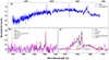 |
Fig. B.1. Mean-normalized 6dF spectrum, taken on 7th February 2005; it is not flux calibrated. A broad Hβ line is not detected; the dashed black line represents the profile corresponding to the upper limit on the amplitude of a broad Gaussian centered near Hβ. This upper limit is comparable to the noise seen in the spectrum, thus barring us from claiming any detection of broad Hβ emission. |
All Tables
Best-fitting parameters from diskline fits to the broad Balmer profiles in the Keck spectrum.
Best-fitting [O III]λ5007, Hβ broad and narrow, [N II]λ6585, Hα broad and narrow emission line fluxes, and RHβ/[O III]
All Figures
|
Fig. 1. Optical, UV, and X-ray light curves for the entire period of our monitoring. From top to bottom, we show (a) 0.2–5.0 keV flux from Swift-XRT, XMM-Newton-EPIC, and eROSITA, (b) UVM2- and UVW1-band flux densities from Swift-UVOT and XMM-Newton-OM, and (c) line fluxes for the broad Hβ and Hα emission components, integrated over the whole broad profile (Sect. 4.4.1). (d) ZTF g- and r-band, (e) ATLAS c- and o-band, (f) WISE W1 and W2 bands. In panels (a), (b), (d), and (e), there are some data points for which the error bars are smaller than the marker for the data point. |
| In the text | |
|
Fig. 3. Broadband SED fits for (a) the first Swift SED, taken near the flare peak in February 2020, and (b) the first XMM-Newton SED, taken in February 2022, assuming a black hole mass of MBH = 4 × 10⁸ M⊙. In each plot, the dashed blue line denotes the intrinsic unabsorbed AGN continuum. The dotted black line denotes the stellar contribution of the host galaxy. The solid black line denotes the Galaxy-absorbed total (AGN + host galaxy) model. The green markers represent the X-ray data and the magenta markers represent optical data. In each panel, the y-error bars are smaller for some data points than the data point marker. |
| In the text | |
|
Fig. 2. X-ray spectra and light curves. Panel (a) shows the variation in the three selected X-ray spectra taken during the brightest phase, the minimum flux, and during the second peak. The round markers represent unfolded data and the solid lines represent best-fit model. Black represents the brightest X-ray observation from Swift, magenta represents the minimum flux observation from eROSITA and blue represents the second peak from Swift. Panels (b) and (c) shows the mean-normalized light curves exhibiting short-term variability in the decaying part of the flare, between MJD 58880 to 58920 for 0.2–5.0 keV X-ray and the UVW2 and UVM2 band, respectively. |
| In the text | |
|
Fig. 4. Optical spectra of J0428−00. Panel (a) displays the 6dF spectrum from 2005 (not flux-calibrated), wherein no broad Hβ emission is detected above the continuum. Panel (b) shows the spectra taken during our 2020–2023 campaign. The spectra are not extinction corrected. The grey bands mark telluric absorption bands. |
| In the text | |
|
Fig. 5. Spectroscopic analysis of the extinction-corrected Keck spectrum. Panel (a) displays the local continuum fit. We fit the local continuum around the broad Hβ and broad Hα line regions using a power law plus host-galaxy template. Panel (b) shows the local continuum-subtracted Hβ line region. The best-fitting model consists of red- and blueshifted broad Gaussians to fit the broad Hβ emission profile, as well as Gaussian profiles fit to the narrow [O III]λλ4959,5007 doublet, including two blueshifted components for each line. The narrow gray Gaussian profile coincides with [Fe VII]λ4893 emission, but this identification is tentative (see text for details). Panel (c) shows the local continuum-subtracted Hα line region. The best-fitting model includes red- and blueshifted broad Gaussians to fit the broad Hα profile, as with Hβ. There are also narrow Gaussian profiles fit to the [N II]λλ6548,6584 and [S II]λλ6716,6731 doublets, as well as to narrow Hα. |
| In the text | |
|
Fig. 6. Ratio of the broad Hβ flux to narrow [O III] λ5007 flux, RHβ/[O III], as a function of time for the 2020–2023 spectra. The ratio is plotted using the round blue marker. The dashed blue line represents the approximate trend. The upper limit to RHβ/[O III] from the archival 6dF spectrum is plotted as the dashed red line. The solid horizontal lines denote the boundaries between Seyfert subtypes following Winkler (1992). |
| In the text | |
|
Fig. 7. Diskline model fits to the broad Hα and Hβ emission line profiles – narrow line and continuum subtracted – as described in Section 4.4.2. Hα profile is fit with (a) single diskline and (b) combination of diskline and a Gaussian profile. Hβ profile is fit with (c) single diskline and (d) combination of diskline and a Gaussian profile, with best-fitting parameters independent of those for the Hα profile fit. The dashed line represents the zero flux density level. |
| In the text | |
|
Fig. 8. BPT diagrams (Baldwin et al. 1981) to assess the activity in J0428−00. The line ratios (panel a) [N II]λ6583/Hα and (panel b) [S II]λ6717/Hα are plotted against the line ratio [O III]λ5007/Hβ. The classification curves are taken from Kewley et al. (2001), Kauffmann et al. (2003), and Schawinski et al. (2007). |
| In the text | |
|
Fig. 9. Balmer decrement as a function of the accretion rate relative to Eddington for our 2020–2023 optical spectra. The markers indicate the values and the shades on the markers indicate time: a deeper shade indicates an earlier time as shown by the colorbar. |
| In the text | |
|
Fig. B.1. Mean-normalized 6dF spectrum, taken on 7th February 2005; it is not flux calibrated. A broad Hβ line is not detected; the dashed black line represents the profile corresponding to the upper limit on the amplitude of a broad Gaussian centered near Hβ. This upper limit is comparable to the noise seen in the spectrum, thus barring us from claiming any detection of broad Hβ emission. |
| In the text | |
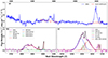 |
Fig. B.2. Same as Fig. 5 but for spectrum S2, taken at LDT on 26 February 2020. |
| In the text | |
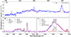 |
Fig. B.3. Same as Fig. 5 but for spectrum S3, taken at LDT on 13 September 2020. |
| In the text | |
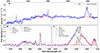 |
Fig. B.4. Same as Fig. 5 but for spectrum S4, taken at LDT on 6 December 2020. |
| In the text | |
Current usage metrics show cumulative count of Article Views (full-text article views including HTML views, PDF and ePub downloads, according to the available data) and Abstracts Views on Vision4Press platform.
Data correspond to usage on the plateform after 2015. The current usage metrics is available 48-96 hours after online publication and is updated daily on week days.
Initial download of the metrics may take a while.