| Issue |
A&A
Volume 702, October 2025
|
|
|---|---|---|
| Article Number | A73 | |
| Number of page(s) | 17 | |
| Section | Cosmology (including clusters of galaxies) | |
| DOI | https://doi.org/10.1051/0004-6361/202553984 | |
| Published online | 14 October 2025 | |
Euclid preparation
LXXIV. Euclidised observations of Hubble Frontier Fields and CLASH galaxy clusters
1
Dipartimento di Fisica “Aldo Pontremoli”, Università degli Studi di Milano, Via Celoria 16, 20133 Milano, Italy
2
INAF-Osservatorio di Astrofisica e Scienza dello Spazio di Bologna, Via Piero Gobetti 93/3, 40129 Bologna, Italy
3
INFN-Sezione di Bologna, Viale Berti Pichat 6/2, 40127 Bologna, Italy
4
Dipartimento di Fisica e Scienze della Terra, Università degli Studi di Ferrara, Via Giuseppe Saragat 1, 44122 Ferrara, Italy
5
INAF-Osservatorio Astronomico di Capodimonte, Via Moiariello 16, 80131 Napoli, Italy
6
INAF-IASF Milano, Via Alfonso Corti 12, 20133 Milano, Italy
7
Universita di Salerno, Dipartimento di Fisica “E.R. Caianiello”, Via Giovanni Paolo II 132, I-84084 Fisciano (SA), Italy
8
INFN – Gruppo Collegato di Salerno – Sezione di Napoli, Dipartimento di Fisica “E.R. Caianiello”, Universita di Salerno, via Giovanni Paolo II, 132 – I-84084 Fisciano (SA), Italy
9
Dipartimento di Fisicae Astronomia “Augusto Righi” – Alma Mater Studiorum Università di Bologna, via Piero Gobetti 93/2, 40129 Bologna, Italy
10
Instituto de Física de Cantabria, Edificio Juan Jordá, Avenida de los Castros, 39005 Santander, Spain
11
Aix-Marseille Université, CNRS, CNES, LAM, Marseille, France
12
Institut d’Astrophysique de Paris, UMR 7095, CNRS, and Sorbonne Université, 98 bis boulevard Arago, 75014 Paris, France
13
STAR Institute, Quartier Agora – Allée du six Août, 19c B-4000 Liège, Belgium
14
Department of Physics, Centre for Extragalactic Astronomy, Durham University, South Road, Durham, DH1 3LE
UK
15
Department of Physics, Institute for Computational Cosmology, Durham University, South Road, Durham, DH1 3LE
UK
16
INAF-Osservatorio Astronomico di Roma, Via Frascati 33, 00078 Monteporzio Catone, Italy
17
Minnesota Institute for Astrophysics, University of Minnesota, 116 Church St SE, Minneapolis, MN 55455
USA
18
Université Paris-Saclay, CNRS, Institut d’astrophysique spatiale, 91405 Orsay, France
19
ESAC/ESA, Camino Bajo del Castillo s/n., Urb. Villafranca del Castillo, 28692 Villanueva de la Cañada, Madrid, Spain
20
School of Mathematics and Physics, University of Surrey, Guildford, Surrey, GU2 7XH
UK
21
INAF-Osservatorio Astronomico di Brera, Via Brera 28, 20122 Milano, Italy
22
IFPU, Institute for Fundamental Physics of the Universe, via Beirut 2, 34151 Trieste, Italy
23
INAF-Osservatorio Astronomico di Trieste, Via G. B. Tiepolo 11, 34143 Trieste, Italy
24
INFN, Sezione di Trieste, Via Valerio 2, 34127 Trieste TS, Italy
25
SISSA, International School for Advanced Studies, Via Bonomea 265, 34136 Trieste TS, Italy
26
Dipartimento di Fisica e Astronomia, Università di Bologna, Via Gobetti 93/2, 40129 Bologna, Italy
27
Max Planck Institute for Extraterrestrial Physics, Giessenbachstr. 1, 85748 Garching, Germany
28
Universitäts-Sternwarte München, Fakultät für Physik, Ludwig-Maximilians-Universität München, Scheinerstrasse 1, 81679 München, Germany
29
INAF-Osservatorio Astrofisico di Torino, Via Osservatorio 20, 10025 Pino Torinese (TO), Italy
30
Dipartimento di Fisica, Università di Genova, Via Dodecaneso 33, 16146 Genova, Italy
31
INFN-Sezione di Genova, Via Dodecaneso 33, 16146 Genova, Italy
32
Department of Physics “E. Pancini”, University Federico II, Via Cinthia 6, 80126 Napoli, Italy
33
INFN section of Naples, Via Cinthia 6, 80126 Napoli, Italy
34
Instituto de Astrofísica e Ciências do Espaço, Universidade do Porto, CAUP, Rua das Estrelas, PT4150-762 Porto, Portugal
35
Faculdade de Ciências da Universidade do Porto, Rua do Campo de Alegre, 4150-007 Porto, Portugal
36
Dipartimento di Fisica, Università degli Studi di Torino, Via P. Giuria 1, 10125 Torino, Italy
37
INFN-Sezione di Torino, Via P. Giuria 1, 10125 Torino, Italy
38
Centro de Investigaciones Energéticas, Medioambientales y Tecnológicas (CIEMAT), Avenida Complutense 40, 28040 Madrid, Spain
39
Port d’Informació Científica, Campus UAB, C. Albareda s/n, 08193 Bellaterra (Barcelona), Spain
40
Institute for Theoretical Particle Physics and Cosmology (TTK), RWTH Aachen University, 52056 Aachen, Germany
41
Institute of Space Sciences (ICE, CSIC), Campus UAB, Carrer de Can Magrans s/n, 08193 Barcelona, Spain
42
Institut d’Estudis Espacials de Catalunya (IEEC), Edifici RDIT, Campus UPC, 08860 Castelldefels, Barcelona, Spain
43
Dipartimento di Fisica e Astronomia “Augusto Righi” – Alma Mater Studiorum Università di Bologna, Viale Berti Pichat 6/2, 40127 Bologna, Italy
44
Instituto de Astrofísica de Canarias, Calle Vía Láctea s/n, 38204 San Cristóbal de La Laguna, Tenerife, Spain
45
Institute for Astronomy, University of Edinburgh, Royal Observatory, Blackford Hill, Edinburgh, EH9 3HJ
UK
46
Jodrell Bank Centre for Astrophysics, Department of Physics and Astronomy, University of Manchester, Oxford Road, Manchester, M13 9PL
UK
47
European Space Agency/ESRIN, Largo Galileo Galilei 1, 00044 Frascati, Roma, Italy
48
Université Claude Bernard Lyon 1, CNRS/IN2P3, IP2I Lyon, UMR 5822, Villeurbanne, F-69100
France
49
Institute of Physics, Laboratory of Astrophysics, Ecole Polytechnique Fédérale de Lausanne (EPFL), Observatoire de Sauverny, 1290 Versoix, Switzerland
50
UCB Lyon 1, CNRS/IN2P3, IUF, IP2I Lyon, 4 rue Enrico Fermi, 69622 Villeurbanne, France
51
Mullard Space Science Laboratory, University College London, Holmbury St Mary, Dorking, Surrey, RH5 6NT
UK
52
Departamento de Física, Faculdade de Ciências, Universidade de Lisboa, Edifício C8, Campo Grande, PT1749-016 Lisboa, Portugal
53
Instituto de Astrofísica e Ciências do Espaço, Faculdade de Ciências, Universidade de Lisboa, Campo Grande, 1749-016 Lisboa, Portugal
54
Department of Astronomy, University of Geneva, ch. d’Ecogia 16, 1290 Versoix, Switzerland
55
INAF-Istituto di Astrofisica e Planetologia Spaziali, via del Fosso del Cavaliere, 100, 00100 Roma, Italy
56
INFN-Padova, Via Marzolo 8, 35131 Padova, Italy
57
Université Paris-Saclay, Université Paris Cité, CEA, CNRS, AIM, 91191 Gif-sur-Yvette, France
58
Istituto Nazionale di Fisica Nucleare, Sezione di Bologna, Via Irnerio 46, 40126 Bologna, Italy
59
INAF-Osservatorio Astronomico di Padova, Via dell’Osservatorio 5, 35122 Padova, Italy
60
Institute of Theoretical Astrophysics, University of Oslo, P.O. Box 1029 Blindern, 0315 Oslo, Norway
61
Jet Propulsion Laboratory, California Institute of Technology, 4800 Oak Grove Drive, Pasadena, CA, 91109
USA
62
Department of Physics, Lancaster University, Lancaster, LA1 4YB
UK
63
Felix Hormuth Engineering, Goethestr. 17, 69181 Leimen, Germany
64
Technical University of Denmark, Elektrovej 327, 2800 Kgs. Lyngby, Denmark
65
Cosmic Dawn Center (DAWN), xxxx, Denmark
66
Max-Planck-Institut für Astronomie, Königstuhl 17, 69117 Heidelberg, Germany
67
Department of Physics and Helsinki Institute of Physics, Gustaf Hällströmin katu 2, University of Helsinki, 00014 Helsinki, Finland
68
Aix-Marseille Université, CNRS/IN2P3, CPPM, Marseille, France
69
Université de Genève, Département de Physique Théorique and Centre for Astroparticle Physics, 24 quai Ernest-Ansermet, CH-1211 Genève 4, Switzerland
70
Department of Physics, P.O. Box 64 University of Helsinki, 00014 Helsinki, Finland
71
Helsinki Institute of Physics, Gustaf Hällströmin katu 2, University of Helsinki, Helsinki, Finland
72
European Space Agency/ESTEC, Keplerlaan 1, 2201 AZ Noordwijk, The Netherlands
73
NOVA optical infrared instrumentation group at ASTRON, Oude Hoogeveensedijk 4, 7991PD Dwingeloo, The Netherlands
74
Centre de Calcul de l’IN2P3/CNRS, 21 avenue Pierre de Coubertin, 69627 Villeurbanne Cedex, France
75
INFN-Sezione di Milano, Via Celoria 16, 20133 Milano, Italy
76
Universität Bonn, Argelander-Institut für Astronomie, Auf dem Hügel 71, 53121 Bonn, Germany
77
INFN-Sezione di Roma, Piazzale Aldo Moro, 2 – c/o Dipartimento di Fisica, Edificio G. Marconi, 00185 Roma, Italy
78
Université Côte d’Azur, Observatoire de la Côte d’Azur, CNRS, Laboratoire Lagrange, Bd de l’Observatoire, CS 34229, 06304 Nice cedex 4, France
79
Université Paris Cité, CNRS, Astroparticule et Cosmologie, 75013 Paris, France
80
Institut d’Astrophysique de Paris, 98bis Boulevard Arago, 75014 Paris, France
81
Institut de Física d’Altes Energies (IFAE), The Barcelona Institute of Science and Technology, Campus UAB, 08193 Bellaterra (Barcelona), Spain
82
School of Mathematics, Statistics and Physics, Newcastle University, Herschel Building, Newcastle-upon-Tyne, NE1 7RU
UK
83
Department of Physics and Astronomy, University of Aarhus, Ny Munkegade 120, DK-8000 Aarhus C, Denmark
84
Space Science Data Center, Italian Space Agency, via del Politecnico snc, 00133 Roma, Italy
85
Centre National d’Etudes Spatiales – Centre spatial de Toulouse, 18 avenue Edouard Belin, 31401 Toulouse Cedex 9, France
86
Institute of Space Science, Str. Atomistilor, nr. 409 Măgurele, Ilfov, 077125
Romania
87
Departamento de Astrofísica, Universidad de La Laguna, 38206 La Laguna, Tenerife, Spain
88
Dipartimento di Fisica e Astronomia “G. Galilei”, Università di Padova, Via Marzolo 8, 35131 Padova, Italy
89
Institut für Theoretische Physik, University of Heidelberg, Philosophenweg 16, 69120 Heidelberg, Germany
90
Institut de Recherche en Astrophysique et Planétologie (IRAP), Université de Toulouse, CNRS, UPS, CNES, 14 Av. Edouard Belin, 31400 Toulouse, France
91
Université St Joseph; Faculty of Sciences, Beirut, Lebanon
92
Departamento de Física, FCFM, Universidad de Chile, Blanco Encalada 2008, Santiago, Chile
93
Satlantis, University Science Park, Sede Bld, 48940 Leioa-Bilbao, Spain
94
Infrared Processing and Analysis Center, California Institute of Technology, Pasadena, CA, 91125
USA
95
Instituto de Astrofísica e Ciências do Espaço, Faculdade de Ciências, Universidade de Lisboa, Tapada da Ajuda, 1349-018 Lisboa, Portugal
96
Universidad Politécnica de Cartagena, Departamento de Electrónica y Tecnología de Computadoras, Plaza del Hospital 1, 30202 Cartagena, Spain
97
INFN-Bologna, Via Irnerio 46, 40126 Bologna, Italy
98
Kapteyn Astronomical Institute, University of Groningen, PO Box 800 9700 AV Groningen, The Netherlands
99
Dipartimento di Fisica, Università degli studi di Genova, and INFN-Sezione di Genova, via Dodecaneso 33, 16146 Genova, Italy
100
INAF, Istituto di Radioastronomia, Via Piero Gobetti 101, 40129 Bologna, Italy
101
Astronomical Observatory of the Autonomous Region of the Aosta Valley (OAVdA), Loc. Lignan 39, I-11020 Nus (Aosta Valley), Italy
102
ICL, Junia, Université Catholique de Lille, LITL, 59000 Lille, France
103
ICSC – Centro Nazionale di Ricerca in High Performance Computing, Big Data e Quantum Computing, Via Magnanelli 2, Bologna, Italy
104
Instituto de Física Teórica UAM-CSIC, Campus de Cantoblanco, 28049 Madrid, Spain
105
CERCA/ISO, Department of Physics, Case Western Reserve University, 10900 Euclid Avenue, Cleveland, OH, 44106
USA
106
Laboratoire Univers et Théorie, Observatoire de Paris, Université PSL, Université Paris Cité, CNRS, 92190 Meudon, France
107
Istituto Nazionale di Fisica Nucleare, Sezione di Ferrara, Via Giuseppe Saragat 1, 44122 Ferrara, Italy
108
Université de Strasbourg, CNRS, Observatoire astronomique de Strasbourg, UMR 7550, 67000 Strasbourg, France
109
Kavli Institute for the Physics and Mathematics of the Universe (WPI), University of Tokyo, Kashiwa, Chiba, 277-8583
Japan
110
Dipartimento di Fisica – Sezione di Astronomia, Università di Trieste, Via Tiepolo 11, 34131 Trieste, Italy
111
NASA Ames Research Center, Moffett Field, CA, 94035
USA
112
Bay Area Environmental Research Institute, Moffett Field, California, 94035
USA
113
Institute Lorentz, Leiden University, Niels Bohrweg 2, 2333 CA Leiden, The Netherlands
114
Institute for Astronomy, University of Hawaii, 2680 Woodlawn Drive, Honolulu, HI 96822
USA
115
Department of Physics & Astronomy, University of California Irvine, Irvine, CA, 92697
USA
116
Department of Astronomy & Physics and Institute for Computational Astrophysics, Saint Mary’s University, 923 Robie Street, Halifax, Nova Scotia B3H 3C3
Canada
117
Departamento Física Aplicada, Universidad Politécnica de Cartagena, Campus Muralla del Mar, 30202 Cartagena, Murcia, Spain
118
Department of Physics, Oxford University, Keble Road, Oxford, OX1 3RH
UK
119
CEA Saclay, DFR/IRFU, Service d’Astrophysique, Bât. 709, 91191 Gif-sur-Yvette, France
120
Institute of Cosmology and Gravitation, University of Portsmouth, Portsmouth, PO1 3FX
UK
121
Department of Computer Science, Aalto University, PO Box 15400 Espoo, FI-00 076
Finland
122
Ruhr University Bochum, Faculty of Physics and Astronomy, Astronomical Institute (AIRUB), German Centre for Cosmological Lensing (GCCL), 44780 Bochum, Germany
123
DARK, Niels Bohr Institute, University of Copenhagen, Jagtvej 155, 2200 Copenhagen, Denmark
124
Instituto de Astrofísica de Canarias (IAC), Departamento de Astrofísica, Universidad de La Laguna (ULL), 38200 La Laguna, Tenerife, Spain
125
Université PSL, Observatoire de Paris, Sorbonne Université, CNRS, LERMA, 75014 Paris, France
126
Université Paris-Cité, 5 Rue Thomas Mann, 75013 Paris, France
127
Univ. Grenoble Alpes, CNRS, Grenoble INP, LPSC-IN2P3, 53, Avenue des Martyrs, 38000 Grenoble, France
128
Department of Physics and Astronomy, Vesilinnantie 5, University of Turku, 20014 Turku, Finland
129
Serco for European Space Agency (ESA), Camino bajo del Castillo s/n, Urbanizacion Villafranca del Castillo, Villanueva de la Cañada, 28692 Madrid, Spain
130
ARC Centre of Excellence for Dark Matter Particle Physics, Melbourne, Australia
131
Centre for Astrophysics & Supercomputing, Swinburne University of Technology, Hawthorn, Victoria 3122, Australia
132
School of Physics and Astronomy, Queen Mary University of London, Mile End Road, London, E1 4NS
UK
133
Department of Physics and Astronomy, University of the Western Cape, Bellville, Cape Town, 7535
South Africa
134
ICTP South American Institute for Fundamental Research, Instituto de Física Teórica, Universidade Estadual Paulista, São Paulo, Brazil
135
Oskar Klein Centre for Cosmoparticle Physics, Department of Physics, Stockholm University, Stockholm, SE-106 91
Sweden
136
Astrophysics Group, Blackett Laboratory, Imperial College London, London, SW7 2AZ
UK
137
INAF-Osservatorio Astrofisico di Arcetri, Largo E. Fermi 5, 50125 Firenze, Italy
138
Dipartimento di Fisica, Sapienza Università di Roma, Piazzale Aldo Moro 2, 00185 Roma, Italy
139
Centro de Astrofísica da Universidade do Porto, Rua das Estrelas, 4150-762 Porto, Portugal
140
Institute of Astronomy, University of Cambridge, Madingley Road, Cambridge, CB3 0HA
UK
141
Department of Astrophysics, University of Zurich, Winterthurerstrasse 190, 8057 Zurich, Switzerland
142
Theoretical astrophysics, Department of Physics and Astronomy, Uppsala University, Box 515 751 20 Uppsala, Sweden
143
Department of Physics, Royal Holloway, University of London, Surrey, TW20 0EX
UK
144
Department of Physics and Astronomy, University of California, Davis, CA, 95616
USA
145
Department of Astrophysical Sciences, Peyton Hall, Princeton University, Princeton, NJ, 08544
USA
146
Cosmic Dawn Center (DAWN)
147
Niels Bohr Institute, University of Copenhagen, Jagtvej 128, 2200 Copenhagen, Denmark
148
Center for Cosmology and Particle Physics, Department of Physics, New York University, New York, NY, 10003
USA
149
Center for Computational Astrophysics, Flatiron Institute, 162 5th Avenue, 10010 New York, NY, USA
⋆ Corresponding author: This email address is being protected from spambots. You need JavaScript enabled to view it.
Received:
31
January
2025
Accepted:
16
June
2025
Abstract
We present HST2EUCLID, a novel Python code to generate Euclid realistic mock images in the HE, JE, YE, and IE photometric bands based on panchromatic Hubble Space Telescope observations. The software was used to create a simulated database of Euclid images for the 27 galaxy clusters observed during the Cluster Lensing And Supernova survey with Hubble (CLASH) and the Hubble Frontier Fields (HFF) program. Since the mock images were generated from real observations, they incorporate, by construction, all the complexity of the observed galaxy clusters. The simulated Euclid data of the galaxy cluster MACS J0416.1−2403 were then used to explore the possibility of developing strong lensing models based on the Euclid data. In this context, complementary photometric or spectroscopic follow-up campaigns are required to measure the redshifts of multiple images and cluster member galaxies. By Euclidising six parallel blank fields obtained during the HFF program, we provide an estimate of the number of galaxies detectable in Euclid images per deg2 per magnitude bin (number counts) and the distribution of the galaxy sizes. Finally, we present a preview of the Chandra Deep Field South that will be observed during the Euclid Deep Survey and two examples of galaxy-scale strong lensing systems residing in regions of the sky covered by the Euclid Wide Survey. The methodology developed in this work lends itself to several additional applications, as simulated Euclid fields based on HST (or JWST) imaging with extensive spectroscopic information can be used to validate the feasibility of legacy science cases or to train deep learning techniques in advance, thus preparing for a timely exploitation of the Euclid Survey data.
Key words: gravitational lensing: strong / galaxies: clusters: general / cosmology: observations / dark matter
Deceased.
© The Authors 2025
 Open Access article, published by EDP Sciences, under the terms of the Creative Commons Attribution License (https://creativecommons.org/licenses/by/4.0), which permits unrestricted use, distribution, and reproduction in any medium, provided the original work is properly cited.
This article is published in open access under the Subscribe to Open model. This email address is being protected from spambots. You need JavaScript enabled to view it. to support open access publication.
1. Introduction
Galaxy clusters, the most powerful gravitational lenses in the Universe, can distort dozens of background sources simultaneously, producing gravitational arcs and multiple images (e.g. Bergamini et al. 2021). Researchers routinely use these features to constrain the total mass distribution in cluster cores.
Various algorithms, including parametric and free form methods, have been developed for this task (e.g. Kneib et al. 1993; Bradač et al. 2005; Diego et al. 2005; Liesenborgs et al. 2006; Coe et al. 2008; Jullo et al. 2007; Zitrin & Broadhurst 2009; Oguri 2010; Zitrin et al. 2013; Lam et al. 2014). Parametric models represent the cluster’s total mass distribution as a collection of mass components, each characterised by parameters varied to fit the strong lensing constraints. These components account for cluster-scale dark matter haloes and the galaxy-scale substructure traced by cluster member galaxies. In contrast, the free-form approach often employs meshes or radial-basis functions to depict the cluster’s total mass distributions. Several of these techniques are discussed and compared in Meneghetti et al. (2017). Bergamini et al. (2019) suggested combining strong lensing with stellar velocity dispersion measurements of cluster galaxies, obtained from the Multi Unit Spectroscopic Explorer (MUSE, at the Very Large Telescope, Bacon et al. 2012) spectra, to enhance the precision of mass models on smaller scales (see also Bergamini et al. 2021; Meneghetti et al. 2020, 2022, 2023; Granata et al. 2022). These additional data help reduce degeneracies between large- and small-scale cluster mass components. Accurate reconstruction of the inner cluster mass distribution is essential for enabling a variety of astrophysical and cosmological applications of strong lensing by galaxy clusters, including studying the nature of dark matter, examining the interplay between baryons and dark matter, exploring cosmic structure formation and evolution, constraining cosmological parameters, and utilising galaxy clusters as cosmic telescopes (see Kneib & Natarajan 2011; Meneghetti et al. 2013; Bartelmann et al. 2013; Moresco et al. 2022, for extensive reviews).
Until recently, only a few tens of galaxy clusters could be accurately modelled for their total mass distributions. Strong lensing modelling requires high spatial resolution and deep observations, previously achievable mainly by the Hubble Space Telescope (HST) and, more recently, the James Webb Space Telescope (JWST). Most known strong lensing clusters were identified in ground-based observations (e.g. Bayliss et al. 2011), or by following up on galaxy clusters pre-selected based on their X-ray emission or the Sunyaev–Zeldovich effect amplitude (Ebeling et al. 2001, 2007, 2010; Planck Collaboration XXVII 2016). Confirming strong lensing features and measuring their redshifts required additional data from the HST (or JWST) and spectrographs on large telescopes.
This situation is set to change dramatically. Since last year, Euclid has been observing most of the extragalactic sky with spatial resolution in the IE band comparable to that of HST (Laureijs et al. 2011; Euclid Collaboration: Scaramella et al. 2022). The Euclid Wide Survey (EWS) aims to cover about 15 000 deg2 of the extragalactic sky to a minimum depth of mAB = 24.5 mag in the IE band (Cropper et al. 2016), with a signal-to-noise ratio (S/N) of 10 for extended sources. Euclid will also survey the same area in the near-infrared YE, JE, and HE bands (Maciaszek et al. 2022) to a depth of mAB = 24.0 mag with a minimum S/N of 5 for point sources. Additionally, its slitless spectroscopy will detect line emission with a sensitivity of fHα ≳ 2 × 10⁻¹⁶ erg s−1cm−2 and a S/N of 3.5 for a typical source of size 0 5.
5.
The primary goal of Euclid is to reveal the nature of dark energy and dark matter, the two dominant components of the Universe, using weak lensing and galaxy clustering as the main probes. However, Euclid will also significantly contribute to the discovery of galaxy clusters. During its lifetime, Euclid is expected to observe over 60 000 galaxy clusters (Sartoris et al. 2016), with a S/N greater than 3, in the redshift range 0.2 ≤ z ≤ 2. About 5000 of these clusters are anticipated to be strong gravitational lenses containing multiple families of lensed images of background sources and strongly distorted radial and tangential arcs (Boldrin et al. 2012, 2016). Developing accurate strong lensing models for even a subset of this large number of cluster lenses will provide critical insights into the nature of dark matter and the growth of cosmic structures, provided that a large number of multiple images and cluster member galaxies can be identified from Euclid observations.
This work introduces a tool to convert HST observations into Euclid-like imaging data. We focus on HST observations of massive galaxy clusters collected in the Cluster Lensing and Supernova Survey with Hubble (CLASH1, Postman et al. 2012) and the Hubble Frontier Fields (HFF2, Lotz et al. 2014, 2017) programmes. We produced a simulated dataset from these images, consisting of mock observations of the same clusters in the EWS. We used simulated observations for the galaxy cluster MACS J0416.1−2403 (hereafter, MACS J0416) to quantify the number of strong lensing features detectable in future Euclid observations of lens galaxy clusters. These are then used to preliminarily test the strengths and weaknesses of Euclid-based cluster strong lensing models. Finally, the HFF parallel fields are employed to estimate the magnitude and size distributions of the luminous sources detectable in the Euclid images.
The paper is organised as follows. In Sect. 2, we present the HST observational dataset used as input for the simulations. The simulation pipeline is detailed in Sect. 3. In Sect. 4, we describe various tests conducted on the mock Euclid images to validate the simulations. In Sect. 5, we present Euclid-based strong lensing models for the galaxy cluster MACS J0416, and the results of the strong lensing analysis are reported in Sect. 6. In Sect. 7, we discuss other applications of the Euclid simulated images, and the main conclusions of this work are outlined in Sect. 8. Throughout this work, magnitudes are given in the AB system (Oke & Gunn 1983).
2. Input data
The simulated Euclid database of galaxy cluster observations presented in this work is based on the photometric data collected by the HST during the CLASH and HFF programmes. The former is a multi-cycle treasury programme that provided panchromatic images of 25 massive galaxy clusters in the redshift range [0.187, 0.890], for a total of 524 orbits from November 2010 to July 2013. The observations were carried out in 16 photometric bands ranging from UV to NIR wavelengths, using the Advanced Camera for Surveys (ACS, with filters: F435W, F475W, F606W, F625W, F775W, F814W, and F850W) and the Wide-Field Camera-3 (WFC3, with filters: F105W, F110W, F125W, F140W, F160W, F225W, F275W, F336W, and F390W). The HFF programme provided deeper HST observations (840 HST orbits) of six massive clusters (four in common with CLASH), selected among the strongest known gravitational lenses, in seven ACS (F435W, F606W, and F814W) and WFC3 (F105W, F125W, F140W, and F160W) bands. The depth of the HFF images corresponds to a limiting magnitude of mAB ∼ 29 with a S/N of 5 for point sources within an aperture of 0 2 radius. This depth is about 1.5 magnitudes deeper than the CLASH observations.
We note that the HFF and CLASH imaging is much deeper than the Euclid observations we wish to produce, as discussed in the following sections. The images used in this work are drizzled to pixel scales of 65 mas px−1 and 60 mas px−1 for the CLASH and HFF data, respectively.
3. Simulation pipeline
This section describes the Python3 code HST2EUCLID developed to simulate realistic Euclid images from HST multi-band observations. Although our primary use in this work is the production of mock Euclid observations of galaxy clusters, HST2EUCLID is generally applicable to convert every sufficiently deep HST image into a Euclid-like observation, with the only requirement being that the available HST bands overlap with the Euclid photometric filters to be simulated (see Fig. 1). In particular, the HST F606W and F814W filters were used to simulate the EuclidIE band, while from the HST F105W, F125W, and F160W filters we simulate the YE, JE, and HE bands (see Sect. 3.3). In Sect. 6, we present selected examples of Euclid observations different from galaxy cluster fields.
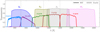 |
Fig. 1. Transmission curves of HST and Euclid filters considered in this work. The five HST filters F606W, F814W, F105W, F125W, and F160W are shown with coloured solid lines, while the four Euclid bands IE, YE, JE, and HE are represented by the coloured areas. The vertical black dashed lines indicate the wavelengths where the response of the HST F814W, F125W, and F160W filters begins to dominate over the F606W, F105W, and F125W filters, respectively. |
Figure 2 visually summarises the different steps of the simulation pipeline (labelled a to e) implemented in the HST2EUCLID code. These are described in detail in the following subsections, adopting the same letters as in Fig. 2, for clarity.
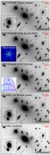 |
Fig. 2. Steps of the Euclidisation pipeline. In the top panel (a), we show the original Hubble F606W image of the galaxy cluster MACS J0416 at z = 0.396. The bottom panel (e) shows the final simulated IE band. The intermediate panels (b), (c), and (d), from top to bottom, illustrate: the convolution to match the Euclid PSF, the result of combining the Hubble F606W and F814W filters to produce the IE band, and the re-binning necessary to match the Euclid pixel scale in the IE band (see Sect. 3). |
3.1. STEP a: Conversion of HST images to flux densities and image alignment
In this first step of the Euclidisation pipeline, we converted the pixel values of the HST images from units of electrons per second (e s−1) to physical flux densities (erg s−1 cm−2 Hz−1). The conversion was performed using the following equation:
![Mathematical equation: $$ \begin{aligned} f[\mathrm{erg}\,\mathrm{s}^{-1}\,\mathrm{cm}^{-2}\,\mathrm{Hz}^{-1}] =F [\mathrm{e}\,\mathrm{s}^{-1}] \times 10^{-0.4\,\left({\mathrm{ZP}_{\rm HST}+48.6}\right)}, \end{aligned} $$](/articles/aa/full_html/2025/10/aa53984-25/aa53984-25-eq3.gif) (1)
(1)
where ZPHST is the instrumental HST zero point, defined as the AB magnitude of an object producing a signal of one electron per second in the HST image. The ZPHST value was computed from the pivot wavelength (PHOTPLAM) and the inverse sensitivity (PHOTFLAM), whose values are provided in the header of the HST Flexible Image Transport System (FITS, Pence et al. 2010) files. Specifically, we used4:
 (2)
(2)
Subsequently, we co-aligned the HST images in the different bands so that they shared the same pixel grid and astrometric calibration. For this purpose, we used the Python function reproject_exact of the module reproject5.
3.2. STEP b: Matching the HST and Euclid point spread functions
The HST point spread functions (PSFs) have different shapes and full width at half maximum (FWHM) compared with the corresponding Euclid PSFs6. These differences must be taken into account to simulate realistic Euclid observations. For each HST band, we derived a kernel function (hereafter, matching kernel) which, when convolved with the corresponding HST images, reproduced the correct PSF in the Euclid simulated data.
The matching kernels between corresponding pairs of HST and Euclid PSFs (see Sect. 3.3) were computed using the Python function create_matching_kernel of the Photutils package (Bradley et al. 2023)7. The HST PSF models were obtained with the TinyTim software8. Although we verified that these PSFs yielded accurate results, HST2EUCLID allows users full flexibility to implement alternative or customised PSF models. In panel (b) of Fig. 2, we show the effect of convolving the HST/F606W image of the galaxy cluster MACS J0416 with the corresponding matching kernel (shown in the inset of the same panel) to the IE band.
3.3. STEP c: Combination of HST filters to generate the Euclid bands
In this step, we expressed the flux in a Euclid band Q as a linear combination of N fluxes in nearby HST filters {Rj}:
 (3)
(3)
where the final term is expressed in linear algebra notation, with w and FR denoting column vectors. Below, we derive an expression for the weight vector w.
We assumed that the spectral density of flux f(λ), – defined as the energy per unit time, per unit spherical angle, per unit detector area, per unit wavelength emitted by a source, (or f(ν) if it is expressed in terms of unit frequency) – could be described as a linear combination of N base functions {fi(λ)} (or {fi(ν)}):
 (4)
(4)
Here, ki are constants associated with the decomposition of the spectral flux density. In computing the last term, we note that fi(λ) can be expressed as a function of frequency as
 (5)
(5)
with c being the light velocity in vacuum. We can then express both FQ and FRj as
 (6)
(6)
where the matrix ℛ is associated with the transmissivity of the HST filters, as detailed below. Assuming the AB magnitude system, all quantities above can be computed as (see Eq. (4) of Hogg et al. 2002)
 (7)
(7)
 (8)
(8)
where gνAB is the zero point for the AB magnitude system (gνAB = 3631 Jy, where 1 Jy = 10−26 W m−2 Hz−1), and Rj(λ) and Q(λ) are the transmissivities of the HST and Euclid photometric bandpasses, respectively (see Fig. 1).
By combining the two expressions in Eq. (6), we obtained9
 (9)
(9)
Finally, by inserting this equation into Eq. (3), we derived the following general expression for the weights:
 (10)
(10)
In Fig. 1, we present the transmission functions of the Euclid photometric bands (IE, YE, JE, and HE, Euclid Collaboration: Schirmer et al. 2022) along with the HST filters used for simulations that cover a similar wavelength range to Euclid (F606W, F814W, F105W, F125W, and F160W). The figure highlights that the wavelength range of the YE band is well aligned with the HST F105W filter, while the HE band overlaps solely with the F160W filter. For both cases, we assumed that the spectral density of flux per unit frequency, f(ν), of the sources in the images remains constant over the entire wavelength range covered by the input (R1) and output (Q1) filters, i.e. f(λ)∝c/λ2. For the HE band, this assumption, necessitated by the absence of HST data covering the reddest part of the HE band (see Fig. 1), is crucial to correctly recovering the measured magnitudes of the luminous sources in the simulated field. However, this represents a rough approximation of the true flux in the real HE band, as it lacks photometric information from the source spectra at λ > 17000 Å. Notably, Balmer break galaxies at redshift z > 3 would appear brighter in HE than in the F160W band. Under the previous assumption, ℛ and q are one-dimensional matrices with  and w = 1. Thus, the magnitudes of the sources in the YE and HEEuclid bands are identical to those in the F105W and F160W HST filters, respectively.
In contrast, the IE and JE transmission functions span two HST bands. Specifically, the IE band overlaps with both the F606W and F814W filters, while the JE band overlaps with the F125W and F160W filters. In these cases, the weights, w, were computed by assuming that the spectral density of flux, f(λ), could be modelled as a sum of two top-hat functions f{1, 2}(ν) (see Eq. (4)). The f1(ν) base function is assumed to be constant within one of the two input HST bands and zero outside, while the opposite holds for f2(ν). In this scenario, ℛ is a two-dimensional matrix with ℛ ∝ 𝕀, where 𝕀 represents the identity matrix, and the weights, wj, assume the following values:
 (11)
(11)
We note that, according to the previous hypotheses, the weights corresponding to the same Euclid band sum to one. In panel (c) of Fig. 2, we show the result of combining the two HST F606W and F814W filters into a single image, obtained using Eq. (3).
3.4. STEP d: Projection onto the Euclid pixel grid
In this step, we re-binned the images from the HST pixel grid to the correct Euclid pixel scale. To this aim, we employed the Python function reproject_exact introduced above. The resulting images have pixel scales of 100 mas px−1 in the IE band and 300 mas px−1 in YE, JE, and HE filters.
The re-binned images, expressed in units of physical flux, were then converted into units of electrons per second by inverting Eq. (1). For this conversion, we assumed a zero point of ZPEuclid = 23.9 mag for all bands. The resulting surface brightness per pixel in the Euclid band X is hereafter denoted as FX, rebin. Panel (d) of Fig. 2 illustrates the result of the re-binning procedure for the IE band.
3.5. STEP e: Noise addition
The final step of the Euclidisation pipeline involved incorporating the appropriate noise into the Euclid simulated images. To accomplish this, we assumed that the noise in the input HST background subtracted images was negligible compared to the final noise. This approximation is supported by the significantly greater depth of the HST observations compared to that of the Euclid images.
The noise level was determined by adjusting the sky surface brightness of the Euclid images to achieve the expected nominal S/N for a source with a specific limiting magnitude. Specifically, to measure a S/N of SNlim for a source with flux of Flim [e s−1] measured within an aperture containing  pixels, the sky surface brightness per pixel in units of [e s−1] was calculated as
![Mathematical equation: $$ \begin{aligned} \mathrm{BK}_{\mathrm{sky} }[\mathrm{e}\,\mathrm{s}^{-1}]&= \left\{ \left(F_{\mathrm{lim} }[\mathrm{e}\,\mathrm{s}^{-1}]\right)^2 \times t_{\mathrm{exp} } \times \left(\mathrm{SN}_{\mathrm{lim} }\right)^{-2}-F_{\mathrm{lim} }[\mathrm{e}\,\mathrm{s}^{-1}]\right\} \nonumber \\&\quad \times \left(N^{\mathrm{px} }_{\mathrm{ap} }\right)^{-1}, \end{aligned} $$](/articles/aa/full_html/2025/10/aa53984-25/aa53984-25-eq16.gif) (12)
(12)
where texp is the exposure time of the Euclid observations. In the EWS, this corresponds to 2280 s for the IE band and 448 s for the YE, JE, and HE bands (Euclid Collaboration: Scaramella et al. 2022). The limiting flux, Flim, was computed from the limiting magnitude, mlim, using the zero point introduced in Sect. 3.4:
![Mathematical equation: $$ \begin{aligned} F_{\mathrm{lim} }[\mathrm{e}\,\mathrm{s}^{-1}] = 10^{0.4\left(\mathrm{ZP} _\mathrm{Euclid} -m_{\mathrm{lim} }\right)}. \end{aligned} $$](/articles/aa/full_html/2025/10/aa53984-25/aa53984-25-eq17.gif) (13)
(13)
The expected limiting magnitudes and S/N in the EWS are reported in Table 1 (Euclid Collaboration: Scaramella et al. 2022). The noise was generated using a Poisson process, where the noise variance is equal to the sum of FX, rebin and BKsky. Panel (e) of Fig. 2 shows the resulting simulated Euclid image in the IE band, including the noise.
Relevant quantities of the EWS.
Fig. 3 presents the results of applying the simulation pipeline, from step (a) to (e), to create mock Euclid observations in all the photometric bands for a region with an approximate size of 70″ × 50″ encompassing the core of the galaxy cluster MACS J0416. The left-hand panels show the input HST photometric data (excluding the HST F814W filter) while the right-hand panels show the output simulated Euclid images in the IE, YE, JE, and HE bands. Despite the shallower depth of the EWS observations compared to the CLASH and HFF observations, many strong lensing features, including some prominent gravitational arcs, are clearly visible in the Euclid images. Notably, the higher spatial resolution of the IE band allowed us to distinguish small details, such as stellar clumps and spiral structures, which appear in some of the multiple images of background lensed galaxies. These features are fundamental in constraining the total mass distribution of galaxy clusters through strong gravitational lensing (e.g. Bergamini et al. 2021; Pignataro et al. 2021), as discussed in subsequent sections. Simulated Euclid images similar to those presented in this section were created for all 27 galaxy clusters observed during the CLASH and HFF programmes.
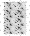 |
Fig. 3. Images of the galaxy cluster MACS J0416 in different photometric filters, observed with HST (left column) and Euclid (right column). The Euclid images are simulated using the pipeline described in Sect. 3, starting from the HST observations in the left column panels including the F814W filter, which is not displayed. |
4. Simulation validation
This section discusses three tests performed on the mock Euclid images to validate the simulation pipeline. In the first test, we verified that the expected depth of the EWS observations was correctly reproduced in the simulations. In the second, we derived the distribution of the sizes of the galaxies in blank fields. Finally, in the third test, we estimated the number counts of galaxies detected in the Euclid images. For tests two and three, we made use of simulated IE images of six cluster-parallel blank fields obtained during the HFF observations.
The coloured dots in the left panel of Fig. 4 show the measured S/N for the luminous sources identified in the different Euclid bands of the galaxy cluster MACS J0416, plotted as a function of their magnitude. These sources include cluster members and galaxies in the cluster foreground or background. Both the S/N and the magnitudes were measured within circular apertures containing 132.7 pixels for the IE band and 9 pixels for the YE, JE, and HE filters (see Table 1). The figure shows that for source magnitude values equal to the limiting magnitude, the measured S/N precisely matches the expected EWS value (dashed coloured lines; see also Table 1). This test demonstrates that the noise in the simulated Euclid images reproduces the expected depth of the EWS data.
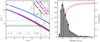 |
Fig. 4. Left: Signal-to-noise ratio (S/N) as a function of the magnitude for the luminous sources detected in the Euclid simulated images of the galaxy cluster MACS J0416. Blue, green, grey, and magenta dots indicate the S/N for galaxies detected in the EuclidIE, YE, JE, and HE images, respectively, as a function of their magnitude in the different bands. These quantities are measured within circular apertures of radius 0 |


The right panel of Fig. 4 shows the distribution of the circularised FWHM for 1748 galaxies, with IE magnitudes ≤ 24.5 (i.e. down to the limiting magnitude), identified in the IE images of the six Euclidised parallel fields described above. The cumulative probability distribution is also plotted in red. This analysis reveals that 93.8% of the selected galaxies have  , with a median value of 0
 59. Assuming a Gaussian profile for the galaxy surface brightness distribution and a median FWHM equal to 0
 59, we find that 96.4% of the brightness of the galaxies is enclosed within an aperture of 0
 65 radius. This value corresponds to the size of the aperture used to measure the limiting magnitude and S/N in the IE band (see Table 1).
Finally, Fig. 5 shows the measured distribution of number counts, i.e. the number of detected galaxies per deg2 per magnitude bin, in the six HFF parallel fields. In the figure, the Euclid number counts (grey histogram) are compared with those estimated from HST observations (black curve, Capak et al. 2007). From the cumulative distribution of galaxies (red dashed line), we estimate that the density of resolved galaxies brighter than the limiting magnitude (IE magnitude ≤24.5) is equal to 28 ± 1 galaxies per arcmin2, in full agreement with expectations for the EWS observations (Laureijs et al. 2011).
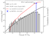 |
Fig. 5. Galaxy number counts from Euclid observations. The galaxy differential number counts derived from the simulated Euclid observations in the IE band of the six HFF parallel fields are shown by the grey histogram with error bars. For comparison, those measured from HST observations (Capak et al. 2007) are indicated by the black solid line. The vertical blue line marks the limiting magnitude in the IE band (24.5 at 10 σ). The cumulative number of galaxies per arcmin2 is shown by the red dashed line. We estimate the number counts from a total area of ∼32.67 arcmin2. We quote the number of galaxies per arcmin2 at the limiting magnitude at the top of the blue vertical line. |
5. Parametric strong lensing models of galaxy clusters based on Euclid observations
As a possible application of the simulated Euclid photometric images, we present a preliminary analysis to quantify the precision and accuracy achievable by parametric strong lensing models of galaxy clusters based on Euclid data. Our analysis focuses on the HFF galaxy cluster MACS J0416, for which Bergamini et al. (2023) developed a high-precision strong lensing model (hereafter the B23 model), based on the spectrophotometric data obtained with HST and MUSE. Both the B23 model and the other lens models presented in this work are constructed using the publicly available parametric software LensTool (Jullo et al. 2007; Limousin et al. 2005; Jullo & Kneib 2009).
In the B23 model, the total projected gravitational potential of MACS J0416 is expressed as the sum of several contributions, each corresponding to a different mass component:
 (14)
(14)
The ϕihalo terms represent the contribution from Nh = 4 cluster-scale haloes to the total cluster gravitational potential. Three of these haloes are parametrised as elliptical dual pseudo-isothermal mass distributions (dPIEs, Limousin et al. 2005; Elíasdóttir et al. 2007; Bergamini et al. 2019) with an infinite truncation radius: two are centred close to the positions of the two brightest cluster galaxies (BCGs), and one is located in the southern part of the cluster, providing second-order corrections to the total mass distribution in that region. The fourth halo is a circular, non-truncated, dPIE profile that accounts for an overdensity of galaxies in the north-eastern region of the cluster. In addition to these cluster-scale haloes, NG = 4 dPIEs (ϕjgas in Eq. (14)) are used to describe the hot gas content of the cluster. The values of the parameters of these profiles are fixed in the B23 lens model, as they were determined from the analysis of Chandra X-ray data of the cluster performed by Bonamigo et al. (2018). The sub-halo mass component of MACS J0416 (corresponding to the terms ϕkgal in Eq. (14)) comprises a total of Ng = 213 cluster member galaxies, including the two BCGs. Of these galaxies, 212 are parametrised as circular, core-less dPIEs, whose central velocity dispersions (σ0) and truncation radii (rcut) are scaled with their luminosities, following the two scaling relations reported in Eq. (4) of Bergamini et al. (2023). The remaining galaxy, identified as Gal-8971, is separately parametrised as an elliptical, core-less dPIE since its total mass is responsible for the formation of a galaxy-galaxy strong lensing system that creates four multiple images of a background source at z = 3.221. Finally, the last term in Eq. (14), ϕfg, accounts for the contribution to the lensing observables from a single foreground galaxy in the southwestern region of the cluster. This galaxy is described as a circular core-less dPIE.
The optimal values of the free parameters of the profiles defined in Eq. (14) were determined by minimising the following χ2 function, which quantifies how well the lens model predicts the observed positions of the multiple images:
 (15)
(15)
where Δxi, j are the uncertainties on the observed positions of the images, Nimj is the number of multiple images of the same j-th background source, and Nsou is the total number of sources. The B23 lens model is constrained by the observed positions of 237 spectroscopically confirmed multiple images from 88 background sources within the redshift range 0.94 ≤ z ≤ 6.63. We refer to Bergamini et al. (2023) for a detailed description of the lens model.
By exploiting the Euclid simulated images of the galaxy cluster MACS J0416 in the IE, YE, JE, and HE bands, we developed two Euclid-based lens models, hereafter identified as EMspec and EMphot. Both EMspec and EMphot assume a parametrisation for the total mass of MACS J0416 similar to that adopted in the B23 model, but with the following three important differences. First, the cluster-scale component of MACS J0416 is parametrised by using just two non-truncated dPIE profiles centred on the positions of the BCGs. Second, the hot-gas mass component is not considered (i.e. the ϕjgas terms are not present in the models). Third, the sub-halo mass component of the cluster contains only those 125 cluster galaxies that are identifiable in the EuclidIE band and with an IE magnitude ≤ 22.5 (see Fig. 6). All these galaxies are parametrised as circular, core-less dPIEs, adopting the σ0–L and rcut–L scaling relations mentioned above, where the luminosity L corresponds to the Kron magnitude of the galaxies measured in the IE band (instead of the HST F160W Kron magnitude adopted in the B23 model). Since Gal-8971 now follows the scaling relations, the number of free parameters in the lens model is reduced by four. Thus, the Euclid-based lens models count a total of 16 free parameters (12 associated with the parametric profiles used to describe the cluster-scale total mass distribution, two are the normalisations of the σ0–L and rcut–L cluster member scaling relations, and two are used to parameterise the foreground galaxy residing in the south-western region of the cluster). We also note that, contrary to the B23 lens model, we did not assume any Gaussian prior on the normalisation of the σ0–L scaling relation. In the B23 model, this Gaussian prior is inferred from the measure stellar kinematics of the cluster member galaxies, through the procedure described by Bergamini et al. (2019).
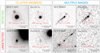 |
Fig. 6. Comparison between cluster members and multiple images as observed by the HST and Euclid. All sources are observed near the core of the galaxy cluster MACS J0416. The upper panels show a cluster member and a lensed galaxy detected in both the HST F160W (HST F606W) and EuclidIE bands. In contrast, the sources in the bottom panels are detected in the HST data but not in the Euclid images. In each panel, we report the IDs of the displayed cluster members and multiple images from the catalogues presented by Bergamini et al. (2023), the F160W total magnitude of the cluster galaxies, and the redshift of the lensed sources. |
The EMspec and EMphot were constrained by the observed positions of 31 multiple images from 12 background sources within the spectroscopic redshift interval 1.01 ≤ z ≤ 2.30. This corresponds to the subsample of multiple images of the original B23 catalogue that were identifiable through visual inspecting the EuclidIE simulated observation. The larger pixel scale and lower resolution and depth of the Euclid images compared to the original HST data allowed the secure detection of 13% of the multiple images used in the B23 model. Figure 6 shows examples of detected and non-detected cluster galaxies and multiple images in the IE image.
The EMspec and EMphot models differ in that, while in the former we used the spectroscopic redshifts of the observed multiple images, in the latter we assumed photometric redshift measurements. To simulate the photometric redshift measurements, we randomly extracted, for each source, a redshift value from a Gaussian distribution centred on the source spectroscopic redshift, zspec, and with a standard deviation equal to (1 + zspec) 0.05. This corresponds to the expected uncertainty on photometric redshift measurements in the EWS (Laureijs et al. 2011; Euclid Collaboration: Desprez et al. 2020; Euclid Collaboration: Paltani et al. 2024).
We note that EMspec and EMphot are optimistic examples of lens models based on Euclid data. To construct these models, we used the multiple images and cluster member catalogues from Bergamini et al. (2023), based on HST photometric data and VIMOS and MUSE spectroscopic data, to identify the sources detectable in the Euclid simulated observations. In more realistic cases, these components for the strong lensing models will be derived solely from the Euclid data. For example, we will identify the cluster galaxies from the observations in the four Euclid bands. Angora et al. (2020) show that this task can be accomplished using convolutional neural networks (CNNs). The proposed technique will be tested with simulated Euclid images obtained with HST2EUCLID in an upcoming paper (Angora et al., in preparation). Spectroscopic follow-up observations will also be critical for identifying pure and complete samples of cluster members and candidate multiple images, as well as for measuring their redshifts. Despite these considerations, our results are informative regarding the precision and accuracy potentially achievable in strong lensing models based on Euclid data. Previous studies, such as those by Johnson & Sharon (2016) and Meneghetti et al. (2017), discuss how the accuracy and precision of strong lensing models depend on the availability of multiple images and spectroscopic redshifts.
6. Results of the strong lensing analysis on the simulated Euclid clusters
To accurately constrain the total mass distribution of galaxy clusters using strong gravitational lensing, it is crucial to determine the positions of a large sample of multiple images from numerous background sources at different redshifts. Likewise, identifying a pure and complete sample of cluster member galaxies is essential for characterising the sub-halo component of the clusters. Additionally, due to degeneracies between lens model parameters, an inaccurate characterisation of the sub-halo mass distribution can introduce biases in determining the other components in Eq. (14).
Figure 7 shows the displacements in the sky plane between the observed and model-predicted positions for the multiple images of the EMspec (red) and EMphot (blue) models compared to those obtained from the reference lens model by Bergamini et al. 2023 (light grey). We quantified the precision of each model in terms of the root-mean-square separation (ΔRMS) between the observed (xobs) and model-predicted (xpre) positions of the multiple images:
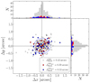 |
Fig. 7. Displacements in the sky plane between the observed and model-predicted positions of the multiple images. We show the results for the models EMspec and EMphot in red and blue, respectively. For comparison, we also show the results obtained by B23 in grey. The histograms show the distribution of the displacements along the two directions. While the B23 model is based on 237 multiple images from 88 background sources, the EMspec and EMphot models are constructed using constraints from 31 multiple images of 12 sources. We quantify the accuracy of each model in terms of the ΔRMS (see Sect. 6), as reported in the legend. This accuracy also determines the radii of the coloured dashed circles in the figure. |
 (16)
(16)
where Nimtot is the total number of images in the model.
The EMphot model is characterised by a  in predicting the positions of the multiple images, which is approximately 33% higher than the other two models. This increased ΔRMS is attributed to weaker lensing constraints from the less accurate photometric redshift measurements, as opposed to spectroscopic redshifts, for the lensed background sources. In contrast, the EMspec predicts the positions of the observed multiple images with a ΔRMS of 0
 39, which is about 9% smaller than for the B23 model (0
 43). This minor discrepancy is due to the differing number of degrees of freedom (DoF, see Eq. (4) in Bergamini et al. 2021) in the two lens models. The EMspec must reproduce the positions of 31 multiple images from 12 background sources (i.e. about 13% of the images considered in the B23 model), using 16 free parameters (22 DoF), whereas the B23 model predicts 237 multiple images from 88 sources with 30 free parameters (268 DoF). Therefore, the considerably higher number of DoF in the latter lens model makes it less prone to overfitting, albeit at the cost of a larger ΔRMS(see Fig. 7).
In Figs. 8 and 9, we compare the convergence and magnification maps obtained from the three lens models. The results are shown on a grid of panels (i, j), where the indices i, j ∈ [1, 3] identify the lens models. Thus, the maps from the i-th lens model are displayed along the diagonal (i = j) of the figures. The model names are reported at the bottom of each column and on the left side of each row of panels. The panels in the i−th row and j−th column show the relative differences between the maps of models j and i.
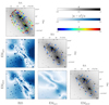 |
Fig. 8. Comparison between the convergence maps for the galaxy cluster MACS J0416, obtained from the B23, EMspec, and EMphot strong lensing models. The maps are rescaled such that the ratio of the lens-source and observer-source angular diameter distances equals one. At the top of each column, we show the convergence maps obtained from the different models, while the dots mark the positions of the multiple images. The latter are colour-coded according to their redshifts. The panels at the intersections between pairs of models show the relative difference between the corresponding convergence maps. |
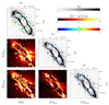 |
Fig. 9. Comparison between the magnification maps of the galaxy cluster MACS J0416, obtained from the B23, EMspec, and EMphot strong lensing models. We show the results for a source at redshift z = 3. The model magnification maps are shown at the top of each column. The dots mark the positions of the multiple images, colour-coded according to their redshifts. The panels at the intersections between pairs of models show the relative differences between the corresponding magnification maps. |
We note that while the convergence maps of the EMspec and EMphot models are quite similar, with a median absolute relative difference of ∼4% (second panel in the bottom row), larger discrepancies exist between these models and the B23 model (first column of panels). This is expected, given the different total mass parametrisations adopted in the Euclid and HST-based lens models. As described in Sect. 5, the large-scale total mass distribution of MACS J0416 in the EMspec and EMphot is parametrised using only two elliptical dPIEs, in contrast to the four included in the B23 model. The two additional haloes in the latter model (a circular one north-east of the northern BCG and a highly elliptical one close to the southern BCG) are clearly identifiable in the panels in the first column of Fig. 8. They correspond to regions of large relative differences between the maps. The models also differ at galaxy scales due to the lower number of cluster galaxies included in the Euclid-based lens models (125 out of 213 in the B23 model), and due to the absence of the Gaussian prior on the value of the normalisation of the σ0–L scaling relation used to model the cluster galaxies (see Sect. 5). In particular, the mass in galaxy-scale haloes in the Euclid-based lens models is larger than in the B23 model (see Fig. 10). Some of the differences between the models are also due to the lack of large-scale haloes describing the hot gas mass distribution in the EMspec and EMphot models.
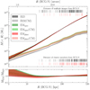 |
Fig. 10. Top panel: Cumulative total mass profiles of MACS J0416 as derived from the B23, EMspec, and EMphot strong lensing models. We show the results for the three models using dark grey, green, and red colours, respectively. The coloured bands indicate the 68.3% confidence intervals. We also show the cumulative total mass profiles for the cluster member component (CM) using lighter colours. The radial distances are measured with respect to the BCG-N. We indicate the positions of multiple images and cluster members used in the Euclid-based and B23 models with red and black vertical sticks at the top and bottom of the figure, respectively. Bottom panel: Ratios between the cumulative total mass profiles derived from the Euclid-based and the B23 models. The coloured bands indicate the 68.3% confidence intervals. |
The Euclid-based models also exhibit similar magnification patterns, as shown in Fig. 9. However, the magnification is derived from the second spatial derivatives of the lensing potential (Meneghetti 2021). Thus, even small differences between the model mass distributions can lead to large variations in magnification on small scales. These variations are most significant along the critical lines, i.e. the lines where the magnification diverges. The differences are larger when the Euclid-based maps are compared to the B23 model. For example, the region along the northern section of the cluster critical lines exhibits large variations between the Euclid-based and B23 models. The EMspec and EMphot models lack constraints in this region. Most of the multiple images detected in the HST data are too faint to be detected by Euclid, as they originate from distant sources at z ≳ 6.
Despite these differences, both the EMspec and EMphot models can be used to accurately measure the total projected mass profile in the cluster core. In the upper panel of Fig. 10, we present the cumulative mass profiles derived from the different lens models. We show profiles for both the total mass distributions and the cluster member (CM) components. We report the ratios between the mass profiles derived from the Euclid-based and B23 models in the bottom panel. The radius R is measured with respect to the position of the northern BCG (BCG-N). The total cumulative mass profiles agree at the level of ≲5% in the radial range covered by the strong lensing constraints, as indicated by the vertical segments at the top of the figure. Significant deviations between the Euclid-based models and the B23 model arise only at distances smaller than ∼ 10 kpc from BCG-N. This result is not surprising, as strong lensing is a robust estimator of the total mass within the Einstein radius (i.e. within the lens critical lines; Meneghetti et al. 2017). However, as highlighted earlier, the Euclid-based models measure a larger mass in cluster members compared to the B23 model. Disentangling the large- and small-scale mass components of the cluster requires additional constraints derived from stellar kinematics measurements (e.g. Bergamini et al. 2019, 2021).
Although not shown in Fig. 10, strong lensing alone is unable to constrain the mass profile far outside the region containing the multiple images. However, due to its large field of view and survey strategy, Euclid will measure the shear out to the virial radius and beyond, at least for massive galaxy clusters (Euclid Collaboration: Giocoli et al. 2024; Euclid Collaboration: Lesci et al. 2024). Several studies have demonstrated that combining weak and strong lensing enhances the precision and accuracy of mass profile measurements out to large radii (e.g. Meneghetti et al. 2010). Moreover, mapping the two-dimensional mass distributions within large regions around the cluster centre allows us to characterise complex mass distributions such as merging clusters and filaments (Bradač et al. 2006; Merten et al. 2011, 2015; Diego et al. 2023).
7. HST2EUCLID applications
Although this work mainly focuses on the analysis of EWS-like data of galaxy clusters, the HST2EUCLID code is designed to simulate customised Euclid imaging observations. In particular, one can use any kind of HST image as an input and specify a number of parameters (exposure times, PSF models, limiting magnitude, and S/N) to generate mock images. As an example, Fig. 11 shows simulated Euclid images of two galaxy-galaxy strong lensing systems, as observed in the EWS. The system shown in the left panels of the figure is identified as SDSS J0946+1006, also known as the Jackpot lens, and consists of a double Einstein ring lensed by a galaxy at z = 0.222 (at the centre of the left images). The inner ring, with a radius of approximately 1 4, has a redshift of z = 0.609, while the outer ring, with a radius of ∼2
 1, has z = 2.035 (Gavazzi et al. 2008). A third source at z = 5.975 is also lensed in two additional multiple images (Collett & Smith 2020). The system shown in the right panels is instead a quadruple imaged quasi-stellar object (QSO) at z = 1.693, lensed by a galaxy at z = 0.455, known as HE0435−1223 (Wisotzki et al. 2002; Bonvin et al. 2017). Fig. 12 shows a simulated preview of a portion of the Chandra Deep Field South (Giacconi et al. 2002) that will be observed in the Euclid Deep Survey (EDS). This simulation assumes an exposure time of 90 744 s and a limiting S/N of 15.9 for a source with an IE magnitude of 26.5, measured within a circular aperture of 0
 65 radius. These values correspond to the EDS expectedrequirements.
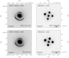 |
Fig. 11. Examples of simulated Euclid images of galaxy-galaxy strong lensing systems as observed during the Euclid wide survey. In the upper panels, we show the two HST images used to generate the simulations in the lower panels. The system on the left, identified as SDSS J0946+1006 (also known as the Jackpot lens), consists of a double Einstein ring lensed by a galaxy at z = 0.222 (at the centre of the image). The HE0435−1223 system on the right is a quadruple imaged quasi-stellar object (QSO) at z = 1.693 lensed by a galaxy at z = 0.455. |
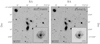 |
Fig. 12. Comparison between a 150″ × 150″ portion of the Chandra Deep Field South as seen by HST (real data) or Euclid (simulated). An exposure time of 90 744 s and a limiting magnitude of 26.5, corresponding to the expected depth of the Euclid deep fields, is assumed in the simulation. |
Since HST2EUCLID is fully modular, it can be easily generalised to simulate a wide range of imaging data. Although this work focuses on converting HST to Euclid data, the software can be extended to include multiple input and output instruments, provided that the input images have higher spatial resolution and depth than the simulated output observations. In this context, the new JWST and the future Extremely Large Telescope (ELT) data can be used to generate the simulations. The JWST data can also be used to fully cover the HE filter as discussed inSect. 3.3.
Another possible application of the HST2EUCLID code, beyond testing the accuracy of Euclid-based strong lensing models, is the search for transient sources (e.g. supernovae and active galactic nuclei) in previously observed HST (or JWST) fields. In particular, a direct comparison between the upcoming real Euclid data and simulated images allows the identification of transient sources by subtracting the simulated images (before the addition of noise; step d of the simulation pipeline presented in Sect. 3 and Fig. 2) from the real observations of the same region. This application is particularly useful for identifying multiple imaged variable sources lensed by galaxy clusters, such as lensed supernovae. The time delays measured between multiple images of these sources can then be used to constrain cosmological parameter values through the time-delaycosmography technique (e.g. Grillo et al. 2020; Treu et al. 2022; Acebron et al. 2023).
In addition, HST2EUCLID can be used to provide the training set for CNN-based techniques aimed at identifying cluster members, galaxy-scale lensing systems, and strong lensing features in clusters (e.g. Angora et al. 2020, 2023; Bazzanini et al., in prep.). More generally, mock HST fields with extensive spectroscopic information are crucial for validating the performance of Euclid across a range of legacy science cases (e.g. the search for high-z dropout galaxies and morphological characterisation of galaxies at variousredshifts).
8. Conclusions
In this article, we present the HST2EUCLID code developed to create simulated Euclid images in the IE, YE, JE, and HE bands using real HST observations in the ACS F606W, ACS F814W, WFC3 F105W, WFC3 F125W, and WFC3 F160W filters. The code is written entirely in Python and can be easily customised for a wide range of studies that make use of Euclid images. A high-level interface based on textual input files allows users to access the full functionalities of the code. As a preliminary application, we used HST2EUCLID to simulate EWS data for 27 clusters observed by the HST during the CLASH and HFF surveys (21 CLASH and 6 HFF clusters). The cluster redshifts range from 0.19 to 0.89.
By using the simulated Euclid images of the galaxy cluster MACS J0416, we tested the possibility of developing high-precision strong lensing models of galaxy clusters based on Euclid data. Our results demonstrate that the Euclid-based lens models are sufficiently accurate to yield precise estimates of the total mass within the cluster critical lines.
The precision and accuracy achievable with Euclid-based lens models rely on the identification of multiple images and cluster members. Both types of sources serve as inputs for constructing the lens models. In this context, redshift measurements from spectroscopic follow-up campaigns will be essential. However, machine and deep learning techniques can automate the search for these sources. Given the paucity of known lenses, especially on the scale of galaxy clusters, training deep learning models requires realistic and sophisticated image simulations, which HST2EUCLID can deliver. For instance, strongly lensed galaxies can be injected into Euclidised HST images to construct a training set (Angora et al., in prep.; Bazzanini et al., in prep.).
Despite our work mainly focusing on analysing EWS-like data of galaxy clusters, the HST2EUCLID code is designed to simulate any kind of Euclid imaging data.
The FWHM values of the HST PSFs in the F606W, F814W, F105W, F125W, and F160W filters range from approximately 70 mas to 130 mas. These values are smaller than those of the Euclid bands at comparable wavelengths (for example, Euclid Collaboration: Mellier et al. 2025 report a measured PSF FWHM of 130 mas in the IE band). Therefore, we can reliably match the HST resolution to that of Euclid by convolving the HST images with the appropriate matching kernels.
A necessary condition for the matrix ℛ to be invertible is that the number of input filters has to be equal to the number of fi(λ) functions in Eq. (4) (i.e. ℛ has to be a square matrix).
Acknowledgments
We acknowledge financial support through grants PRIN-MIUR 2017WSCC32 and 2020SKSTHZ. PB acknowledges financial support from ASI through the agreement ASI-INAF n. 2018-29-HH.0. MM acknowledges support from the Italian Space Agency (ASI) through contract “Euclid – Phase E” and “Euclid – Phase D”. LB is indebted to the communities behind the multiple free, libre, and open-source software packages on which we all depend on. The Euclid Consortium acknowledges the European Space Agency and a number of agencies and institutes that have supported the development of Euclid, in particular the Agenzia Spaziale Italiana, the Austrian Forschungsförderungsgesellschaft funded through BMK, the Belgian Science Policy, the Canadian Euclid Consortium, the Deutsches Zentrum für Luft- und Raumfahrt, the DTU Space and the Niels Bohr Institute in Denmark, the French Centre National d’Etudes Spatiales, the Fundação para a Ciência e a Tecnologia, the Hungarian Academy of Sciences, the Ministerio de Ciencia, Innovación y Universidades, the National Aeronautics and Space Administration, the National Astronomical Observatory of Japan, the Netherlandse Onderzoekschool Voor Astronomie, the Norwegian Space Agency, the Research Council of Finland, the Romanian Space Agency, the State Secretariat for Education, Research, and Innovation (SERI) at the Swiss Space Office (SSO), and the United Kingdom Space Agency. A complete and detailed list is available on the Euclid web site (www.euclid-ec.org/). This work uses the following software packages: Astropy (Astropy Collaboration 2013, 2018), matplotlib (Hunter 2007), Numpy (van der Walt et al. 2011; Harris et al. 2020), Python (Van Rossum & Drake 2009), Scipy (Virtanen et al. 2020), acstools (Lim et al. 2020), reproject, argparse, re, pickle, os, photutils (Bradley et al. 2023).
References
- Acebron, A., Schuldt, S., Grillo, C., et al. 2023, A&A, 680, L9 [NASA ADS] [CrossRef] [EDP Sciences] [Google Scholar]
- Angora, G., Rosati, P., Brescia, M., et al. 2020, A&A, 643, A177 [NASA ADS] [CrossRef] [EDP Sciences] [Google Scholar]
- Angora, G., Rosati, P., Meneghetti, M., et al. 2023, A&A, 676, A40 [NASA ADS] [CrossRef] [EDP Sciences] [Google Scholar]
- Astropy Collaboration (Robitaille, T. P., et al.) 2013, A&A, 558, A33 [NASA ADS] [CrossRef] [EDP Sciences] [Google Scholar]
- Astropy Collaboration (Price-Whelan, A. M., et al.) 2018, AJ, 156, 123 [Google Scholar]
- Bacon, R., Accardo, M., Adjali, L., et al. 2012, Messenger, 147, 4 [NASA ADS] [Google Scholar]
- Bartelmann, M., Limousin, M., Meneghetti, M., & Schmidt, R. 2013, Space Sci. Rev., 177, 3 [NASA ADS] [CrossRef] [Google Scholar]
- Bayliss, M. B., Hennawi, J. F., Gladders, M. D., et al. 2011, ApJS, 193, 8 [Google Scholar]
- Bergamini, P., Rosati, P., Mercurio, A., et al. 2019, A&A, 631, A130 [NASA ADS] [CrossRef] [EDP Sciences] [Google Scholar]
- Bergamini, P., Rosati, P., Vanzella, E., et al. 2021, A&A, 645, A140 [EDP Sciences] [Google Scholar]
- Bergamini, P., Grillo, C., Rosati, P., et al. 2023, A&A, 674, A79 [NASA ADS] [CrossRef] [EDP Sciences] [Google Scholar]
- Boldrin, M., Giocoli, C., Meneghetti, M., & Moscardini, L. 2012, MNRAS, 427, 3134 [NASA ADS] [CrossRef] [Google Scholar]
- Boldrin, M., Giocoli, C., Meneghetti, M., et al. 2016, MNRAS, 457, 2738 [CrossRef] [Google Scholar]
- Bonamigo, M., Grillo, C., Ettori, S., et al. 2018, ApJ, 864, 98 [Google Scholar]
- Bonvin, V., Courbin, F., Suyu, S. H., et al. 2017, MNRAS, 465, 4914 [NASA ADS] [CrossRef] [Google Scholar]
- Bradač, M., Schneider, P., Lombardi, M., & Erben, T. 2005, A&A, 437, 39 [NASA ADS] [CrossRef] [EDP Sciences] [Google Scholar]
- Bradač, M., Clowe, D., Gonzalez, A. H., et al. 2006, ApJ, 652, 937 [CrossRef] [Google Scholar]
- Bradley, L., Sipőcz, B., Robitaille, T., et al. 2023, https://doi.org/10.5281/zenodo.7946442 [Google Scholar]
- Capak, P., Aussel, H., Ajiki, M., et al. 2007, ApJS, 172, 99 [Google Scholar]
- Coe, D., Fuselier, E., Benítez, N., et al. 2008, ApJ, 681, 814 [NASA ADS] [CrossRef] [Google Scholar]
- Collett, T. E., & Smith, R. J. 2020, MNRAS, 497, 1654 [NASA ADS] [CrossRef] [Google Scholar]
- Cropper, M., Pottinger, S., Niemi, S., et al. 2016, in Space Telescopes and Instrumentation 2016: Optical, Infrared, and Millimeter Wave, eds. H. A. MacEwen, G. G. Fazio, M. Lystrup, et al., Society of Photo-Optical Instrumentation Engineers (SPIE) Conference Series, 9904, 99040Q [NASA ADS] [Google Scholar]
- Diego, J. M., Protopapas, P., Sandvik, H. B., & Tegmark, M. 2005, MNRAS, 360, 477 [Google Scholar]
- Diego, J. M., Meena, A. K., Adams, N. J., et al. 2023, A&A, 672, A3 [NASA ADS] [CrossRef] [EDP Sciences] [Google Scholar]
- Ebeling, H., Edge, A. C., & Henry, J. P. 2001, ApJ, 553, 668 [Google Scholar]
- Ebeling, H., Barrett, E., Donovan, D., et al. 2007, ApJ, 661, L33 [Google Scholar]
- Ebeling, H., Edge, A. C., Mantz, A., et al. 2010, MNRAS, 407, 83 [NASA ADS] [CrossRef] [Google Scholar]
- Elíasdóttir, Á., Limousin, M., Richard, J., et al. 2007, arXiv e-prints [arXiv:0710.5636] [Google Scholar]
- Euclid Collaboration (Desprez, G., et al.) 2020, A&A, 644, A31 [EDP Sciences] [Google Scholar]
- Euclid Collaboration (Giocoli, C., et al.) 2024, A&A, 681, A67 [NASA ADS] [CrossRef] [EDP Sciences] [Google Scholar]
- Euclid Collaboration (Lesci, G. F., et al.) 2024, A&A, 684, A139 [NASA ADS] [CrossRef] [EDP Sciences] [Google Scholar]
- Euclid Collaboration (Mellier, Y., et al.) 2025, A&A, 697, A1 [Google Scholar]
- Euclid Collaboration (Paltani, S., et al.) 2024, A&A, 681, A66 [NASA ADS] [CrossRef] [EDP Sciences] [Google Scholar]
- Euclid Collaboration (Scaramella, R., et al.) 2022, A&A, 662, A112 [NASA ADS] [CrossRef] [EDP Sciences] [Google Scholar]
- Euclid Collaboration (Schirmer, M., et al.) 2022, A&A, 662, A92 [NASA ADS] [CrossRef] [EDP Sciences] [Google Scholar]
- Gavazzi, R., Treu, T., Koopmans, L. V. E., et al. 2008, ApJ, 677, 1046 [NASA ADS] [CrossRef] [Google Scholar]
- Giacconi, R., Zirm, A., Wang, J., et al. 2002, ApJS, 139, 369 [Google Scholar]
- Granata, G., Mercurio, A., Grillo, C., et al. 2022, A&A, 659, A24 [NASA ADS] [CrossRef] [EDP Sciences] [Google Scholar]
- Grillo, C., Rosati, P., Suyu, S. H., et al. 2020, ApJ, 898, 87 [Google Scholar]
- Harris, C. R., Millman, K. J., van der Walt, S. J., et al. 2020, Nature, 585, 357 [NASA ADS] [CrossRef] [Google Scholar]
- Hogg, D. W., Baldry, I. K., Blanton, M. R., & Eisenstein, D. J. 2002, arXiv e-prints [arXiv:astro-ph/0210394] [Google Scholar]
- Hunter, J. D. 2007, Comput. Sci. Eng., 9, 90 [NASA ADS] [CrossRef] [Google Scholar]
- Johnson, T. L., & Sharon, K. 2016, ApJ, 832, 82 [Google Scholar]
- Jullo, E., & Kneib, J.-P. 2009, MNRAS, 395, 1319 [Google Scholar]
- Jullo, E., Kneib, J.-P., Limousin, M., et al. 2007, New J. Phys., 9, 447 [Google Scholar]
- Kneib, J.-P., & Natarajan, P. 2011, A&ARv, 19, 47 [Google Scholar]
- Kneib, J., Mellier, Y., Fort, B., & Mathez, G. 1993, A&A, 273, 367 [Google Scholar]
- Lam, D., Broadhurst, T., Diego, J. M., et al. 2014, ApJ, 797, 98 [NASA ADS] [CrossRef] [Google Scholar]
- Laureijs, R., Amiaux, J., Arduini, S., et al. 2011, arXiv e-prints [arXiv:1110.3193] [Google Scholar]
- Liesenborgs, J., De Rijcke, S., & Dejonghe, H. 2006, MNRAS, 367, 1209 [NASA ADS] [CrossRef] [Google Scholar]
- Lim, P. L., Davis, M., Hack, W., et al. 2020, Astrophysics Source Code Library [record ascl:2011.024] [Google Scholar]
- Limousin, M., Kneib, J.-P., & Natarajan, P. 2005, MNRAS, 356, 309 [Google Scholar]
- Lotz, J., Mountain, M., Grogin, N. A., et al. 2014, American Astronomical Society Meeting Abstracts, 223, 254.01 [Google Scholar]
- Lotz, J. M., Koekemoer, A., Coe, D., et al. 2017, ApJ, 837, 97 [Google Scholar]
- Maciaszek, T., Ealet, A., Gillard, W., et al. 2022, in Space Telescopes and Instrumentation 2022: Optical, Infrared, and Millimeter Wave, eds. L. E. Coyle, S. Matsuura, & M. D. Perrin, Society of Photo-Optical Instrumentation Engineers (SPIE) Conference Series, 12180, 18 [Google Scholar]
- Meneghetti, M. 2021, Introduction to Gravitational Lensing: With Python Examples, Lecture Notes in Physics (Springer International Publishing) [Google Scholar]
- Meneghetti, M., Rasia, E., Merten, J., et al. 2010, A&A, 514, A93 [NASA ADS] [CrossRef] [EDP Sciences] [Google Scholar]
- Meneghetti, M., Bartelmann, M., Dahle, H., & Limousin, M. 2013, Space Sci. Rev., 177, 31 [NASA ADS] [CrossRef] [Google Scholar]
- Meneghetti, M., Natarajan, P., Coe, D., et al. 2017, MNRAS, 472, 3177 [Google Scholar]
- Meneghetti, M., Davoli, G., Bergamini, P., et al. 2020, Science, 369, 1347 [Google Scholar]
- Meneghetti, M., Ragagnin, A., Borgani, S., et al. 2022, A&A, 668, A188 [NASA ADS] [CrossRef] [EDP Sciences] [Google Scholar]
- Meneghetti, M., Cui, W., Rasia, E., et al. 2023, A&A, 678, L2 [NASA ADS] [CrossRef] [EDP Sciences] [Google Scholar]
- Merten, J., Coe, D., Dupke, R., et al. 2011, MNRAS, 417, 333 [NASA ADS] [CrossRef] [Google Scholar]
- Merten, J., Meneghetti, M., Postman, M., et al. 2015, ApJ, 806, 4 [Google Scholar]
- Moresco, M., Amati, L., Amendola, L., et al. 2022, Liv. Rev. Relat., 25, 6 [NASA ADS] [Google Scholar]
- Oguri, M. 2010, PASJ, 62, 1017 [NASA ADS] [Google Scholar]
- Oke, J. B., & Gunn, J. E. 1983, ApJ, 266, 713 [NASA ADS] [CrossRef] [Google Scholar]
- Pence, W. D., Chiappetti, L., Page, C. G., Shaw, R. A., & Stobie, E. 2010, A&A, 524, A42 [NASA ADS] [CrossRef] [EDP Sciences] [Google Scholar]
- Pignataro, G. V., Bergamini, P., Meneghetti, M., et al. 2021, A&A, 655, A81 [NASA ADS] [CrossRef] [EDP Sciences] [Google Scholar]
- Planck Collaboration XXVII. 2016, A&A, 594, A27 [NASA ADS] [CrossRef] [EDP Sciences] [Google Scholar]
- Postman, M., Coe, D., Benítez, N., et al. 2012, ApJS, 199, 25 [Google Scholar]
- Sartoris, B., Biviano, A., Fedeli, C., et al. 2016, MNRAS, 459, 1764 [Google Scholar]
- Treu, T., Suyu, S. H., & Marshall, P. J. 2022, A&ARv, 30, 8 [NASA ADS] [CrossRef] [Google Scholar]
- van der Walt, S., Colbert, S. C., & Varoquaux, G. 2011, Comput. Sci. Eng., 13, 22 [Google Scholar]
- Van Rossum, G., & Drake, F. L. 2009, Python 3 Reference Manual (Scotts Valley, CA: CreateSpace) [Google Scholar]
- Virtanen, P., Gommers, R., Oliphant, T. E., et al. 2020, Nat. Methods, 17, 261 [Google Scholar]
- Wisotzki, L., Schechter, P. L., Bradt, H. V., Heinmüller, J., & Reimers, D. 2002, A&A, 395, 17 [NASA ADS] [CrossRef] [EDP Sciences] [Google Scholar]
- Zitrin, A., & Broadhurst, T. 2009, ApJ, 703, L132 [NASA ADS] [CrossRef] [Google Scholar]
- Zitrin, A., Meneghetti, M., Umetsu, K., et al. 2013, ApJ, 762, L30 [NASA ADS] [CrossRef] [Google Scholar]
All Tables
All Figures
|
Fig. 1. Transmission curves of HST and Euclid filters considered in this work. The five HST filters F606W, F814W, F105W, F125W, and F160W are shown with coloured solid lines, while the four Euclid bands IE, YE, JE, and HE are represented by the coloured areas. The vertical black dashed lines indicate the wavelengths where the response of the HST F814W, F125W, and F160W filters begins to dominate over the F606W, F105W, and F125W filters, respectively. |
| In the text | |
|
Fig. 2. Steps of the Euclidisation pipeline. In the top panel (a), we show the original Hubble F606W image of the galaxy cluster MACS J0416 at z = 0.396. The bottom panel (e) shows the final simulated IE band. The intermediate panels (b), (c), and (d), from top to bottom, illustrate: the convolution to match the Euclid PSF, the result of combining the Hubble F606W and F814W filters to produce the IE band, and the re-binning necessary to match the Euclid pixel scale in the IE band (see Sect. 3). |
| In the text | |
|
Fig. 3. Images of the galaxy cluster MACS J0416 in different photometric filters, observed with HST (left column) and Euclid (right column). The Euclid images are simulated using the pipeline described in Sect. 3, starting from the HST observations in the left column panels including the F814W filter, which is not displayed. |
| In the text | |
|
Fig. 4. Left: Signal-to-noise ratio (S/N) as a function of the magnitude for the luminous sources detected in the Euclid simulated images of the galaxy cluster MACS J0416. Blue, green, grey, and magenta dots indicate the S/N for galaxies detected in the EuclidIE, YE, JE, and HE images, respectively, as a function of their magnitude in the different bands. These quantities are measured within circular apertures of radius 0 |
| In the text | |
|
Fig. 5. Galaxy number counts from Euclid observations. The galaxy differential number counts derived from the simulated Euclid observations in the IE band of the six HFF parallel fields are shown by the grey histogram with error bars. For comparison, those measured from HST observations (Capak et al. 2007) are indicated by the black solid line. The vertical blue line marks the limiting magnitude in the IE band (24.5 at 10 σ). The cumulative number of galaxies per arcmin2 is shown by the red dashed line. We estimate the number counts from a total area of ∼32.67 arcmin2. We quote the number of galaxies per arcmin2 at the limiting magnitude at the top of the blue vertical line. |
| In the text | |
|
Fig. 6. Comparison between cluster members and multiple images as observed by the HST and Euclid. All sources are observed near the core of the galaxy cluster MACS J0416. The upper panels show a cluster member and a lensed galaxy detected in both the HST F160W (HST F606W) and EuclidIE bands. In contrast, the sources in the bottom panels are detected in the HST data but not in the Euclid images. In each panel, we report the IDs of the displayed cluster members and multiple images from the catalogues presented by Bergamini et al. (2023), the F160W total magnitude of the cluster galaxies, and the redshift of the lensed sources. |
| In the text | |
|
Fig. 7. Displacements in the sky plane between the observed and model-predicted positions of the multiple images. We show the results for the models EMspec and EMphot in red and blue, respectively. For comparison, we also show the results obtained by B23 in grey. The histograms show the distribution of the displacements along the two directions. While the B23 model is based on 237 multiple images from 88 background sources, the EMspec and EMphot models are constructed using constraints from 31 multiple images of 12 sources. We quantify the accuracy of each model in terms of the ΔRMS (see Sect. 6), as reported in the legend. This accuracy also determines the radii of the coloured dashed circles in the figure. |
| In the text | |
|
Fig. 8. Comparison between the convergence maps for the galaxy cluster MACS J0416, obtained from the B23, EMspec, and EMphot strong lensing models. The maps are rescaled such that the ratio of the lens-source and observer-source angular diameter distances equals one. At the top of each column, we show the convergence maps obtained from the different models, while the dots mark the positions of the multiple images. The latter are colour-coded according to their redshifts. The panels at the intersections between pairs of models show the relative difference between the corresponding convergence maps. |
| In the text | |
|
Fig. 9. Comparison between the magnification maps of the galaxy cluster MACS J0416, obtained from the B23, EMspec, and EMphot strong lensing models. We show the results for a source at redshift z = 3. The model magnification maps are shown at the top of each column. The dots mark the positions of the multiple images, colour-coded according to their redshifts. The panels at the intersections between pairs of models show the relative differences between the corresponding magnification maps. |
| In the text | |
|
Fig. 10. Top panel: Cumulative total mass profiles of MACS J0416 as derived from the B23, EMspec, and EMphot strong lensing models. We show the results for the three models using dark grey, green, and red colours, respectively. The coloured bands indicate the 68.3% confidence intervals. We also show the cumulative total mass profiles for the cluster member component (CM) using lighter colours. The radial distances are measured with respect to the BCG-N. We indicate the positions of multiple images and cluster members used in the Euclid-based and B23 models with red and black vertical sticks at the top and bottom of the figure, respectively. Bottom panel: Ratios between the cumulative total mass profiles derived from the Euclid-based and the B23 models. The coloured bands indicate the 68.3% confidence intervals. |
| In the text | |
|
Fig. 11. Examples of simulated Euclid images of galaxy-galaxy strong lensing systems as observed during the Euclid wide survey. In the upper panels, we show the two HST images used to generate the simulations in the lower panels. The system on the left, identified as SDSS J0946+1006 (also known as the Jackpot lens), consists of a double Einstein ring lensed by a galaxy at z = 0.222 (at the centre of the image). The HE0435−1223 system on the right is a quadruple imaged quasi-stellar object (QSO) at z = 1.693 lensed by a galaxy at z = 0.455. |
| In the text | |
|
Fig. 12. Comparison between a 150″ × 150″ portion of the Chandra Deep Field South as seen by HST (real data) or Euclid (simulated). An exposure time of 90 744 s and a limiting magnitude of 26.5, corresponding to the expected depth of the Euclid deep fields, is assumed in the simulation. |
| In the text | |
Current usage metrics show cumulative count of Article Views (full-text article views including HTML views, PDF and ePub downloads, according to the available data) and Abstracts Views on Vision4Press platform.
Data correspond to usage on the plateform after 2015. The current usage metrics is available 48-96 hours after online publication and is updated daily on week days.
Initial download of the metrics may take a while.