| Issue |
A&A
Volume 702, October 2025
|
|
|---|---|---|
| Article Number | A4 | |
| Number of page(s) | 32 | |
| Section | Planets, planetary systems, and small bodies | |
| DOI | https://doi.org/10.1051/0004-6361/202554652 | |
| Published online | 30 September 2025 | |
A JWST/MIRI view of κ Andromedae b: Refining its mass, age, and physical parameters
1
Aix Marseille Université, CNRS, CNES, LAM,
Marseille,
France
2
Jet Propulsion Laboratory, California Institute of Technology,
Pasadena,
CA
91109,
USA
3
Department of Physics & Astronomy, Johns Hopkins University,
3400 N. Charles Street,
Baltimore,
MD
21218,
USA
4
Space Telescope Science Institute,
3700 San Martin Drive,
Baltimore,
MD
21218,
USA
5
LIRA, Observatoire de Paris, Université PSL, Sorbonne Université, Université Paris Cité, CY Cergy Paris Université, CNRS,
92190
Meudon,
France
6
Université Paris-Saclay, UVSQ, CNRS, CEA, Maison de la Simulation,
91191
Gif-sur-Yvette,
France
7
INAF – Osservatorio Astrofisico di Arcetri,
Largo E. Fermi 5,
50125
Firenze,
Italy
8
Université Paris-Saclay, Université Paris Cité, CEA, CNRS, AIM,
91191
Gif-sur-Yvette,
France
★ Corresponding author: This email address is being protected from spambots. You need JavaScript enabled to view it.
Received:
19
March
2025
Accepted:
4
August
2025
Abstract
Context. κ And b is a substellar companion with a mass near the planet–brown dwarf boundary orbiting a B9IV star at ~50–100 au. Estimates of its age and mass vary, which has fueled a decade-long debate. Additionally, the atmospheric parameters (Teff 1650–2050 K and log(g) 3.5–5.5 dex) remain poorly constrained. The differences in atmospheric models and inhomogeneous datasets contribute to the varied interpretations.
Aims. We aim to refine the characterization of κ And b by using mid-infrared data to capture its full bolometric emission. Combined with near-infrared (NIR) measurements, we aim to constrain Teff, log(g), and the radius to narrow down the uncertainties in age and mass.
Methods. We obtained JWST/MIRI coronagraphic data in the F1065C, F1140C, and F1550C filters and recalibrated existing NIR photometry using an updated ATLAS stellar model. We used MIRI color–magnitude diagrams to probe the likelihood of species (e.g., CH4, NH3, and silicates). We compared the H and F1140C colors and magnitudes of the companion to isochrones to constrain the age and mass. We then modeled its spectral energy distribution with atmospheric models to refine the estimates of Teff, radius, and log(g) and to constrain age and mass using evolutionary models.
Results. Cloudy atmosphere models fit the spectral energy distribution of κ And b best. This is consistent with its L0/L2 spectral type and its position near silicate-atmosphere field objects in the MIRI color–magnitude diagram. We derived an age of 47 ± 7 Myr and a mass of 17.3 ± 1.8 MJup by weight-mean combining the models. Atmospheric modeling yielded Teff = 1791 ± 68 K and a radius of 1.42 ± 0.06 RJup. This improves the precision by ~30% over previous estimates. log(g) was constrained to 4.35 ± 0.07 dex, which is an improvement in the precision by ~70% relative to the most precise literature value of 4.75 ± 0.25 dex.
Conclusions. Our new mass estimate places κ And b slightly above the planet–brown dwarf boundary determined by the deuterium-burning limit. Our age estimate is ~75% more precise than previous values and aligns the object with the Columba association (42 Myr). The derived Teff suggests silicate clouds, but this needs to be confirmed spectroscopically. MIRI data were crucial to refine the radius and temperature, which led to stronger constraints on the age and mass (both dependent on the model) and improved the overall characterization of κ And b.
Key words: techniques: high angular resolution / planets and satellites: atmospheres / planets and satellites: fundamental parameters / planets and satellites: gaseous planets / infrared: planetary systems
© The Authors 2025
 Open Access article, published by EDP Sciences, under the terms of the Creative Commons Attribution License (https://creativecommons.org/licenses/by/4.0), which permits unrestricted use, distribution, and reproduction in any medium, provided the original work is properly cited.
This article is published in open access under the Subscribe to Open model. This email address is being protected from spambots. You need JavaScript enabled to view it. to support open access publication.
1 Introduction
Planetary-mass companions observed with direct imaging such as HR 2562 b (Mesa et al. 2018), HR 8799 bcde (Marois et al. 2008), and β Pic b (Lagrange et al. 2010) provide unique insights into planet formation mechanisms at wide orbits, including disk instability and core accretion (Spiegel & Burrows 2012. These insights are further supported by statistical analyses from dedicated surveys (e.g., Vigan et al. 2021). These companions offer us the opportunity to study planetary evolution in dynamically complex environments where host star radiation, disk chemistry, and gravitational interactions play a critical role in shaping their atmospheric and orbital properties (e.g., Fortney et al. 2008; Öberg et al. 2011; Marleau & Cumming 2014; Bowler 2016; Nielsen et al. 2019). Unlike isolated brown dwarfs, which are thought to form through cloud fragmentation, planetary-mass companions, particularly those at separations below a few hundred AU, likely form within circumstellar disks and evolve under the influence of their host star and the circumstellar disk. This provides a contrasting perspective on substellar atmospheres and formation histories.
L-type objects, in particular, early L types L0/L2, represent a critical transition regime between low-mass stars, brown dwarfs, and massive planets. Their effective temperatures (~1400–2000 K) and atmospheric conditions make them key for understanding the giant planet formation and atmospheric evolution (e.g., Tremblin et al. 2016), especially during the L to T transition. This phase is characterized by dramatic changes in the cloud structure and spectral appearance because silicate and iron clouds condense below the visible/NIR photosphere (e.g., Cushing et al. 2005; Burrows et al. 2006; Saumon & Marley 2008; Marley et al. 2012; Suárez & Metchev 2022). Thick silicate clouds and iron and alkali metals dominate their spectra. This introduces complexities in modeling their atmospheric properties (e.g., Miles et al. 2023). These challenges make L-type objects, especially planetary companions, pivotal for studying cloud dynamics and chemical disequilibria.
Direct-imaging observations of young planetary-mass companions further highlight their differences from field brown dwarfs, particularly among L-type objects. The low surface gravity, enhanced chemical mixing, and highly cloudy or dusty atmospheres set them apart from brown dwarfs that formed through cloud fragmentation (e.g., Currie et al. 2011; Allers & Liu 2013; De Rosa et al. 2016; Rajan et al. 2017; Chauvin et al. 2017). By capturing their infrared spectra, direct imaging enables us to access their properties while they are still warm and luminous. NIR observations are crucial for constraining bulk parameters such as effective temperature, surface gravity, luminosity, and mass. The limited spectral coverage of ground-based instruments often restricts our ability to fully characterize these objects, but particularly L-types, whose spectral energy distributions (SEDs) challenge atmospheric models because their cloud and chemical processes are complex (e.g., Saumon & Marley 2008, Tremblin et al. 2016).
The combination of NIR and mid-infrared (MIR) observations has proven essential for a more comprehensive characterization of these low-mass objects. MIR observations, particularly from space-based telescopes and observatories such as the James Webb Space Telescope (JWST; Rigby et al. 2023), improve the constraints on effective temperature, surface gravity, and radius (e.g., Carter et al. 2023; Boccaletti et al. 2024; Godoy et al. 2024). These constraints are further enhanced when the system ages are well determined, as was shown for objects from well-dated moving groups such as β Pic (e.g., 20.4 ± 2.5 Myr, Couture et al. 2023) and Columba (e.g., 42 ± 8 Myr, Bell et al. 2015). The uncertainties in the ages can significantly affect the inferred physical properties, however, including the mass and radius. This complicates the differentiation between planetary-mass objects and brown dwarfs (e.g., Carson et al. 2013 and Hinkley et al. 2013). It is essential to address these age-related uncertainties to refine evolutionary models and understand the formation pathways.
The atmospheric characterization of young planetary companions is often hindered by heterogeneous datasets and varying modeling assumptions. The conversion of contrast into absolute magnitudes relies on stellar spectral models that differ from the stellar parameters, which introduces systematic offsets in the companion properties and flux normalization (e.g., Hinkley et al. 2013 vs. Currie et al. 2018). Additionally, differences in the spectral coverage, calibration, and method of the instruments can result in significant discrepancies in the retrieved spectra and physical parameters (e.g., Sutlieff et al. 2021; Nasedkin et al. 2023; Xuan et al. 2022). This highlights the need for uniform analysis pipelines and multi-instrument integration for robust atmospheric constraints.
These challenges are well illustrated by κ Andromedae b. This planetary-mass companion (L0/L2; Uyama et al. 2020) orbits a B9IV star and has been the focus of debate since its discovery (Carson et al. 2013) because of the large uncertainties in the system age. Combined with varying model assumptions and calibration discrepancies, these uncertainties yield a wide range of estimates for its effective temperature, surface gravity, and mass.
We present the first JWST coronagraphic observations of κ And b using the Mid-Infrared Instrument (MIRI; Rieke et al. 2015, Wright et al. 2015) at wavelengths of 10.65 μm, 11.40 μm, and 15.50 μm. These observations were conducted with the advanced coronagraphic abilities of JWST/MIRI (Boccaletti et al. 2015; Danielski et al. 2018; Boccaletti et al. 2022) and provide unprecedented insights into the atmosphere and physical properties of κ And b. They address some of the limitations posed by earlier ground-based observations.
The structure of this paper is as follows: Section 2 provides an overview of the κ Andromedae system and summarizes its key properties and contextual relevance. Section 3 describes the observations and data processing, including the recalibration of archival ground-based observations. Section 4 delves into the analysis of the new data and presents updated estimates of the physical parameters of the companion. Finally, we discuss in Section 5 the broader implications of these findings for understanding planetary-mass companions and their formation mechanisms, which is followed by a summary of our conclusions in Section 6.
Main properties and stellar parameters of the star κ And.
2 The κ Andromedae system
Kappa Andromedae (κ And), also known as HD 222439, HIP 116805, HR 8976, and TYC 3244-1530-1, is a high proper motion and young B9IVn-type star (Garrison & Gray 1994) at ~51 pc (Gaia Collaboration 2020, Gaia Collaboration 2016). In Table 1 we summarize the main stellar parameters known to date, and in Table 2 the magnitudes and fluxes. The star hosts a planetary-mass companion, κ And b, discovered by Carson et al. (2013), at an angular separation of 1″.058 (on 2012 July 8), and semi-major axis of 103.6 AU (57.4–107.4 AU 68% confidence interval, Uyama et al. 2020). We summarize the main properties of the companion later in this section.
The age of the κ And system has been a topic of significant discussion over the past decade. Zuckerman et al. (2011) first proposed that the system is a member of the Columba association (~30 Myr), adopted by Carson et al. (2013) in their analysis of κ And b. Hinkley et al. (2013) questioned the membership of the system in the Columba association, however, and proposed an older isochronal age of 220 ± 100 Myr for the host star. Subsequent studies aimed to refine the system’s age. Bonnefoy et al. (2014) supported a younger age of ![Mathematical equation: $\[30_{-10}^{+120}\]$](/articles/aa/full_html/2025/10/aa54652-25/aa54652-25-eq9.png) Myr based on kinematics and color–magnitude diagram (CMD) coupled with isochrones. Jones et al. (2016) used long-baseline optical interferometry to measure the star’s size, oblateness, and rotation velocity, enabling strong constraints on its age and mass. Combining these with evolutionary models, they derived an age of
Myr based on kinematics and color–magnitude diagram (CMD) coupled with isochrones. Jones et al. (2016) used long-baseline optical interferometry to measure the star’s size, oblateness, and rotation velocity, enabling strong constraints on its age and mass. Combining these with evolutionary models, they derived an age of ![Mathematical equation: $\[47_{-40}^{+27}\]$](/articles/aa/full_html/2025/10/aa54652-25/aa54652-25-eq10.png) Myr, assuming solar metallicity ([M/H] = 0.0). This estimate is consistent with the revised age of the Columba association of
Myr, assuming solar metallicity ([M/H] = 0.0). This estimate is consistent with the revised age of the Columba association of ![Mathematical equation: $\[42_{-4}^{+6}\]$](/articles/aa/full_html/2025/10/aa54652-25/aa54652-25-eq11.png) Myr from Bell et al. (2015). Currie et al. (2018) estimated an age of
Myr from Bell et al. (2015). Currie et al. (2018) estimated an age of ![Mathematical equation: $\[40_{-19}^{+34}\]$](/articles/aa/full_html/2025/10/aa54652-25/aa54652-25-eq12.png) Myr from empirical comparisons, kinematics, and the properties of the host star and companion. Stone et al. (2020) used hot-start evolutionary models and companion data to suggest a broader 10–100 Myr range, while Wilcomb et al. (2020) set an upper limit of 50 Myr based on evolutionary models. Despite differing methods, these studies consistently support a young system age.
Myr from empirical comparisons, kinematics, and the properties of the host star and companion. Stone et al. (2020) used hot-start evolutionary models and companion data to suggest a broader 10–100 Myr range, while Wilcomb et al. (2020) set an upper limit of 50 Myr based on evolutionary models. Despite differing methods, these studies consistently support a young system age.
The ongoing uncertainty in the system’s age has significantly affected the inferred properties of κ And b, in particular its mass estimate. Assuming a younger age of ~30 Myr, Carson et al. (2013) estimated a mass of ![Mathematical equation: $\[12.8_{-1}^{+2}\]$](/articles/aa/full_html/2025/10/aa54652-25/aa54652-25-eq13.png) MJup for the companion, consistent with a planetary-mass object. In contrast, the older age proposed by Hinkley et al. (2013) implied a more massive object (
MJup for the companion, consistent with a planetary-mass object. In contrast, the older age proposed by Hinkley et al. (2013) implied a more massive object (![Mathematical equation: $\[50_{-13}^{+16}\]$](/articles/aa/full_html/2025/10/aa54652-25/aa54652-25-eq14.png) MJup) with a surface gravity consistent with a brown dwarf classification. Jones et al. (2016), using the derived atmospheric models fit parameters from Hinkley et al. (2013), infer a mass of
MJup) with a surface gravity consistent with a brown dwarf classification. Jones et al. (2016), using the derived atmospheric models fit parameters from Hinkley et al. (2013), infer a mass of ![Mathematical equation: $\[22_{-7}^{+6}\]$](/articles/aa/full_html/2025/10/aa54652-25/aa54652-25-eq15.png) MJup. Recent studies, including Currie et al. (2018) and Uyama et al. (2020), found that κ And b exhibits low-gravity features in its spectrum, aligning with an L0–L1 spectral type and a mass of
MJup. Recent studies, including Currie et al. (2018) and Uyama et al. (2020), found that κ And b exhibits low-gravity features in its spectrum, aligning with an L0–L1 spectral type and a mass of ![Mathematical equation: $\[13_{-2}^{+12}\]$](/articles/aa/full_html/2025/10/aa54652-25/aa54652-25-eq16.png) MJup. Gratton et al. (2024), using photometry measurements from Uyama et al. (2020) and an average age of 36 ± 8 Myr, estimate a mass of 15.03 ± 0.66 MJup.
MJup. Gratton et al. (2024), using photometry measurements from Uyama et al. (2020) and an average age of 36 ± 8 Myr, estimate a mass of 15.03 ± 0.66 MJup.
Previous studies inferred the effective temperature and surface gravity of κ And b from its SED using various atmospheric models, datasets, and calibrations, leading to discrepancies in parameter estimates. For instance, temperatures range from ~1600 K (Carson et al. 2013) up to 1900–2040 K (Hinkley et al. 2013; Bonnefoy et al. 2014; Wilcomb et al. 2020), with several studies suggesting intermediate values around 1680–1800 K (Todorov et al. 2016; Currie et al. 2018; Stone et al. 2020; Uyama et al. 2020; Morris et al. 2024; Gratton et al. 2024; Xuan et al. 2024). Surface gravity is less well constrained, with log(g) estimates spanning from ~3.8 to 4.7 dex (Wilcomb et al. 2020; Bonnefoy et al. 2014; Currie et al. 2018; Stone et al. 2020; Uyama et al. 2020; Morris et al. 2024), but with large uncertainties (0.25–1.0 dex) spanning a broad range (3.5–5.5 dex).
The atomic and molecular abundances have also been measured for κ And b, first by Wilcomb et al. (2020), who found C/O = ![Mathematical equation: $\[0.70_{-0.24}^{+0.09}\]$](/articles/aa/full_html/2025/10/aa54652-25/aa54652-25-eq17.png) , and later by Xuan et al. (2024), who reported C/O =
, and later by Xuan et al. (2024), who reported C/O = ![Mathematical equation: $\[0.58_{-0.04}^{+0.05}\]$](/articles/aa/full_html/2025/10/aa54652-25/aa54652-25-eq18.png) and [C/H]=
and [C/H]= ![Mathematical equation: $\[-0.12_{-0.19}^{+0.28}\]$](/articles/aa/full_html/2025/10/aa54652-25/aa54652-25-eq19.png) . The projected rotational velocity v sin(i) was also measured by Morris et al. 2024 as 38.42 ± 0.05 km s−1, and by Xuan et al. (2024) as 39.4 ± 0.9 km s−1.
. The projected rotational velocity v sin(i) was also measured by Morris et al. 2024 as 38.42 ± 0.05 km s−1, and by Xuan et al. (2024) as 39.4 ± 0.9 km s−1.
The spectral type of κ And b is better constrained, ranging consistently from L0 to L2 across multiple studies (Carson et al. 2013; Hinkley et al. 2013; Bonnefoy et al. 2014; Currie et al. 2018; Stone et al. 2020; Uyama et al. 2020), with L3 occasionally included (Stone et al. 2020). This spectral classification helps us to limit the plausible surface gravity range to approximately 3.9–4.5 dex, thereby placing useful constraints on the companion’s atmospheric parameters. Figure 1 shows κ And b’s position on a J-K CMD consistent with the spectral class derived by Uyama et al. (2020, L0/L2).
These studies suggest that the mass and surface gravity estimates of the companion are closely tied to the system age and the wavelength coverage that was used in observations. By probing the system in the MIR, we can gain more accurate insights into these properties, helping to refine the physical characteristics of the companion.
Archival and measured κ And magnitudes and fluxes.
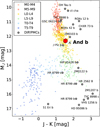 |
Fig. 1 CMD showing the position of κ And b (red hexagon marker) relative to the population of low-mass stars and brown dwarfs (colored circles) as obtained from Best et al. (2021). The different colors highlight the different spectral types. The gray pentagons correspond to selected directly imaged planets (DIP) and planetary-mass companions (PMCs). |
3 Observations and data reduction
3.1 Observations and strategy
The observations of the κ Andromedae system were carried out under the guarantee time observation program 1241 (PI: M. Ressler), using the JWST/MIRI instrument. This program is part of the MIRICLE Collaboration (Boccaletti et al. 2024; Godoy et al. 2024; Mâlin et al. 2024), an agreement between the US and European MIRI team to explore the properties of the known substellar companions with MIRI coronagraphic imaging. The observations were taken on September 19, 2023, within 3.5 hours of execution time. We used the four-quadrant phase mask coronagraphs (4QPMs; Rouan et al. 2000) with the narrow-band filters F1065C (10.57 μm), F1140C (11.3 μm), and F1550C (15.5 μm). The observing strategy is identical to that used for HR 2562 b, as detailed in Godoy et al. (2024), while the exposure parameters were independently optimized using the MIRI Coronagraphic Simulation pipeline (Danielski et al. 2018).
We used reference differential imaging (RDI; Smith & Terrile 1984), given that the roll subtraction (Burrows et al. 1995) would induce excessive self-subtraction of the companion (separation of ~0.7″, Currie et al. 2018). We selected HD 222389, a K5 (Cannon & Pickering 1993) star classified as a long-period variable (P=92.6 ± 2.6 days, ΔV=166 mmag, ΔG=168 mmag; Burggraaff et al. 2018, Lebzelter et al. 2023), located at a distance of ~539 pc (Gaia Collaboration 2016, Gaia Collaboration 2020), as the reference star. We chose this star based on the JWST User Documentation1 and following the same consideration presented in Godoy et al. (2024). We used the dither-pattern technique with the small-grid dither pattern 5-point-small-grid (see Lajoie et al. 2016) in a cross configuration, to accurately subtract the science star coronagraphic point spread function (PSF; e.g., Carter et al. 2023).
Given the presence of the “glow stick” stray light (Boccaletti et al. 2022), we added background observations for the science target and the reference star to allow the subtraction of this feature. The observing setups are shown in Table 3 for the two stars κ And and HD 222389.
3.2 Data reduction and preprocessing
We reduced the data using the JWST2, 3 pipeline routines (version 1.10.0, Bushouse et al. 2022; CRDS version 11.16.21), with the spaceKLIP4 pipeline (version 0.1, Kammerer et al. 2022). We modified some minor aspects in the pipeline to optimize the preprocessing and cosmetics calibrations (see Godoy et al. 2024 for more details). We emphasize that, at the time of our data reduction and post-processing, these improvements were not yet included in the official pipelines, although they have since been incorporated into recent releases. We proceed with stages 1 and 2 as in Godoy et al. (2024), optimizing the initial parameters for the best detection and correction of cosmic rays and bad pixels.
The hit of energetic cosmic rays affected mostly the integrations at F1550C, making the post-processing challenging. Godoy et al. (2024) addressed this issue as a post-reduction by applying custom techniques to identify bad pixels and cosmic ray remnants, which are then corrected using interpolation routines. Instead, we solve this problem as a pre-reduction step, correcting the *uncal* files before starting the data reduction. In short, we compute the flux difference between each consecutive pair of groups within each ramp, and we identify cosmic ray events from any departure above 5 times the median absolute deviation (MAD) flux difference value. The ramp is then corrected by replacing the flux difference between groups affected by the event with the median flux difference along the ramp. In Appendix A, we explain in more detail this procedure. Figure 2 shows an example of the energetic cosmic ray treatment, using an optimized spaceKLIP setup (left) and using our method (right). We observe that certain artifacts, such as the black line in the left image, caused by a cosmic ray, are effectively eliminated using our correction method. We applied the post-reduction correction method described by Godoy et al. (2024) to correct the residual and persistent bad pixels in the reduced images.
For the background subtraction, we first computed the combined background for each target and filter. We employed the “cube structure” method described in Godoy et al. (2024), which achieves superior subtraction compared to mean-combining all background observations. We also used the same procedure as Godoy et al. (2024) for removing the background and the “glow stick” artifacts, which has a considerable impact at F1550C filter.
We note that despite the application of pre- and post-corrections during data reduction, a fringing structure remains in the reference star observations at F1065C and F1140C, characterized by horizontal lines, which significantly impacts the post-processing stage (see Fig. B.1). We attribute the presence of this structure to the small number of groups (seven; see Table 3), selected to prevent saturation. It limits the ability of the pipeline to adequately correct for the detector structure, however. We developed a step-by-step procedure to remove this fringing, starting with the identification of the structure and then applying row normalization to the image. In our example, we reduced the flux dispersion from ~100 to ~50 MJy/str. The complete procedure is detailed in Appendix B. Figure 3 shows an example of an image at F1065C before (left) and after (right) fringing correction. We emphasize that the “fringing structure” is only present in the reference frames (Ngroups=7 vs. Ngroups=28 for the science star), so the correction does not affect the science data after PSF subtraction. Since we processed the data, this “fringing” has been associated with the 390 Hz pattern noise seen in many MIRI sub-array observations, described in the JWST documentation website5. A pipeline correction is now available as part of the emicorr step of the calwebb_detector1 module of the pipeline.
Observational setup.
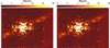 |
Fig. 2 Second integration of the third dither position of the reference star HD 222389 after the BACKGROUND subtraction at the F1550C filter. Left: Frame with the standard data reduction parameters using spaceKLIP. Right: same frame, but directly applying our cosmic-ray and bad-pixel corrections in the raw frame. |
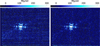 |
Fig. 3 First integration of the third dither position of the reference star HD 222389 after the background subtraction at the F1065C filter. Left: frame with the fringing structure (horizontal lines) after applying the normal reduction. Right: same frame after applying our additional correction procedure, in which we removed the fringing structure. |
3.3 Post-processing, photometry, and contrast
We used the spaceKLIP pipeline to optimally subtract the starlight with principal component analysis (PCA). spaceKLIP uses the stellar spectrum and magnitude to calibrate the contrast and extract the companion photometry. We used the ATLAS/SYNTHE atmospheric models (Kurucz 2013, Kurucz 2014) from VidmaPy6 to generate a synthetic spectrum7 of the star. The stellar parameters and their uncertainties were taken from Table 1 based on Jones et al. (2016), and the spectrum was used as input for spaceKLIP. The model includes the obliquity and the stellar rotation interferometric measurements, which significantly affect the stellar spectrum and spectral lines. We rescaled the spectrum using the new 2MASS magnitudes estimated by Bonnefoy et al. (2014). To validate the stellar model, we collected archival photometry data from Vizier (Ochsenbein et al. 2000), listed in Table 2. We proceeded to generate 1 000 synthetic spectra considering all the parameters and uncertainties using a Monte Carlo approach. At the same time, we calculated the synthetic photometry at each MIRI filter (F1065C, F1140C, and F1550C; see Table 2). From the 1000 synthetic spectra, we computed the mean stellar spectrum that is used in spaceKLIP for contrast calibration, as well as the standard deviation as a representation of the uncertainty. We computed the synthetic photometry in the same manner. Figure 4 shows the SED of κ And, featuring the archival and synthetic photometry and the synthetic spectrum.
For the starlight subtraction, we proceeded in the same way as Godoy et al. (2024). We used the RDI technique to suppress the starlight using PCA. The reference star has 15 integrations coming from the dithering and integrations (see Table 3), so we explored the range of 1 to 15 components. We performed separate optimizations of the starlight subtraction to maximize the detection and flux extraction of the companion, and to derive the contrast limits for each filter. For the companion, we determined that the best extraction is using the “blur” (smooth using a Gaussian kernel) option in the spaceKLIP pipeline. We analyze this point in more detail in Appendix C. Figure 5 shows the best extraction of the companion, obtained with 10,7, and 8 components for the F1065C, F1140C, and F1550C, respectively. We note that at F1550C there are some hot and/or bad pixels at the location of the companion. To determine if our extraction is biased by these pixels, we injected a fake planet with and without bad pixels rotated 180° and at the same angular separation and same brightness (see Appendix D). We conclude that these hot and/or bad pixels do not bias our measurements, since there is a small deviation within the uncertainties of around ~6% compared to the ~17% uncertainty (see Fig. D.1). The measured fluxes of the companion κ And b in the MIRI filters are presented in Table 4. Figure 6 shows the pre- and post-processed frames using the optimal number of components for RDI.
We estimated the contrast limits for each filter using an adaptive approach that optimizes performance at all angular separations. Instead of fixing the number of components, we evaluated contrasts for 1 to 15 components and retained the best contrast at each separation to produce a combined contrast curve (Xuan et al. 2018). The contrast limits were derived directly from post-processed images after extracting the flux of κ And b. These limits were computed accounting for small sample statistics (Mawet et al. 2014). Corrections were applied for coronagraphic transmission and over-subtraction biases introduced by the Karhunen–Loève Image Projection (KLIP), which were quantified by injecting and recovering calibration point sources in the raw and processed images. To reduce noise fluctuations (due to the small-step angular separation used), we first extended the contrast data by stacking it symmetrically and applied a Gaussian window function in the frequency domain using a Fourier transform. Afterward, we performed an inverse Fourier transform to bring the data back to the spatial domain and truncated it to the original length. This allowed us to remove the noise in the contrast curve. Finally, we fitted a polynomial to the smoothed contrast values (reducing the high-frequency fluctuations) to obtain the final contrast curve. The final combined and smoothed contrast limits are presented in Figure 7.
Photometry and astrometry of κ And b derived from the MIRI coronagraphic observations.
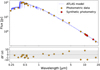 |
Fig. 4 Top: SED of the star κ Andromedae. The orange dots correspond to the photometric data from Table 2. Red dots correspond to our synthetic photometry using the F1065C, F1140C, and F1550C bandpasses. The blue line corresponds to the mean between the 1000 realizations of ATLAS models with the respective uncertainties. Bottom: Residuals between the model and the data. The gray region corresponds to 3σ. |
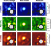 |
Fig. 5 Modeling and extraction of the companion κ And b. From top to bottom: filters F1065C, F1140C, and F1550C. Left: post-processed science images, corresponding to 10,7, and 8 components for the filters F1065C, F1140C, and F1550C, respectively. Middle: best spaceKLIP model of the companion using webb_psf. Right: residuals after subtracting the model from the science data. The field of view corresponds to 25 × 25 pixels (~2.75″ × 2.75″). The images in each row have the same color scale. The gray region with white lines represents a hatched mask corresponding to the star behind the coronagraph. |
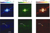 |
Fig. 6 Pre- and post-processing frames of κ And. Top: background-subtracted and stacked science frames. The stacking is only for visualization purposes. Bottom: starlight-subtracted image using RDI and KLIP at the optimal number of components. From left to right: F1065C, F1140C, and F1550C filters. The horizontal white arrow highlights the position of κ And b. Each of the columns (i.e., filters) has the same color scale. The yellow star in each subplot marks the position of the star κ And. North is up and east to the left. |
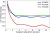 |
Fig. 7 Smoothed contrast limits for all JWST/MIRI κ And observations in the F1065C (blue), F1140C (green), and F1550C (red) bandpasses. |
3.4 Uniform recalibration of archival data
All available observations of the companion κ And b are compiled in Table 5. To avoid biases from inconsistent calibrations and ensure a homogeneous flux calibration across all datasets, we reprocessed and uniformly recalibrated all existing flux measurements of the companion with a unique and state-of-the-art stellar atmospheric model. For all the archival observations, we retrieved the raw, uncalibrated contrast of the companion, along with the instrument filter transmission. We then used the precise stellar model of κ And (see Fig. 4), to compute the stellar flux in the archival data filter bandpasses, and consistently calibrate the raw companion fluxes. Below, we summarize the recalibration for each observation, and Appendix E provides additional details about each calibration. We highlight that the uncertainty associated with our ATLAS spectrum was considered in the calibration of all the datasets.
Carson et al. 2013: Carson et al. observed κ And with the Subaru telescope on 2012 January-July using the HiCIAO (High Contrast Instrument for the Subaru Next Generation Adaptive Optics; Hodapp et al. 2008) and IRCS (Infrared Camera and Spectrograph; Tokunaga et al. 1998) instruments in the J, H, Ks, and L′ bands (see Table 5). They used the 2MASS J, H, and Ks magnitudes for flux calibration to convert the κ And b contrast into apparent magnitudes. We note a difference of about 3% (0.03 in magnitude) between the 2MASS and Subaru/HiCIAO filters. Additionally, as highlighted by Bonnefoy et al. (2014), the 2MASS images are saturated, which leads to incorrect flux measurements for the star κ And. We used our stellar model to compute the 2MASS magnitudes, which agree with the ones reported by Bonnefoy et al. (2014). We then computed the Subaru/HiCIAO J, H, and Ks magnitudes using our stellar models to convert the κ And b contrast into apparent magnitudes.
Hinkley et al. 2013: Hinkley et al. observed κ And using the P1640 instrument at Palomar on 2012 December 23 (Hinkley et al. 2011, Oppenheimer et al. 2012), integral field spectroscopy (IFS) mode (Hinkley et al. 2008) covering the YJH bands. They flux-calibrated the observations using a B9V stellar spectrum model from the Pickles Stellar Library (Pickles 1998). As noted by Currie et al. (2018), the Pickles B9 spectrum shows significant deviations in the NIR with respect to other stellar models (e.g., Kurucz atmospheric models). To correct this, we applied a correction factor by dividing the B9V-calibrated model by our ATLAS stellar spectrum model. Note that the calibrator factor has a dependence on wavelength and it is not a single value. The differences between the Pickles and ATLAS models result in a change in the shape of the IFS spectrum of κ And b (see Figure E.2).
Table 5Corrected magnitudes archival data of κ And b using κ And ATLAS atmospheric model.
Bonnefoy et al. 2014: Bonnefoy et al. observed κ And on 2012 October 6 and 30, and November 3 using the Keck and the Large Binocular Telescope Interferometer (LBTI) observatories in the Ks, L′, Brα, and M′ bands. They also reestimated the 2MASS magnitudes of κ And using a calibrator star on 2012 October 30 with the Mimir instrument (Clemens et al. 2007) mounted on the 1.8m Perkins telescope at Lowell Observatory. We calculated the contrast magnitudes of κ And b and derived the magnitudes in each filter using our stellar spectrum model. The resulting magnitudes are consistent with those from Bonnefoy et al. (2014), with about 0.01 mag differences. We did not re-estimate the L′ magnitude, as it was flux-calibrated using HR 8799, which we consider an unbiased measurement.
Currie et al. 2018: Currie et al. observed κ And using the Subaru SCExAO (Subaru Coronagraphic Extreme AO)/CHARIS integral field spectrograph in the JHK bands (Peters-Limbach et al. 2012; Groff et al. 2014; Groff et al. 2015) on 2017 September 8. To flux-calibrate the IFS data, they used a Kurucz stellar atmosphere model (Castelli & Kurucz 2003) with8 Teff = 11 400 K and log(g)= 4.0 dex. As with the Hinkley et al. (2013) observations, we computed a correction factor by comparing the Kurucz models with our ATLAS spectrum. The correction is small and within the uncertainties, primarily affecting the H-band peak (see Figure E.3). Currie et al. (2018) also highlights that they did not include a 5% uncertainty from the flux calibration, so we incorporated this uncertainty in our correction.
Kühn et al. 2018: They observed κ And as part of the first-light and on-sky commissioning results of the H-band Vector Vortex Coronagraph for the SCExAO System on 2016 November 12. They reported only the κ And b contrast, which is 10.35. This value differs from those reported by Carson et al. (2013) and Currie et al. (2018). We chose not to use this contrast, as it may be biased due to data processing or calibration issues, and it was not reported the related uncertainty which is crucial to determining the possibility of biases.
Wilcomb et al. 2020: They observed κ And with the OSIRIS (OH-Suppressing Infrared Imaging Spectrograph) integral field spectrograph at the Keck Observatory (R~4 000, Larkin et al. 2006) in the K broadband mode on 2016 November 6–8 and 2017 November 4. Wilcomb et al. (2020) did not perform direct flux calibration. To remove telluric absorptions in κ And, b, however, they masked the H lines in κ And and normalized the continuum using a blackbody with the same temperature as determined by Jones et al. (2016). We did not apply any additional corrections at this step since they used the same temperature as our ATLAS model. Then, they calibrated the resulting κ And b spectrum using the K-band apparent magnitude computed by Currie et al. (2018) and a distance of 50.0 ± 0.1 pc. To renormalize the OSIRIS spectrum, we calculated the WIYN/WHIRC9 KsMKO magnitude in the OSIRIS spectrum and in the corrected Currie et al. CHARIS IFS data. Using both, we computed the correction factor to renormalize the OSIRIS spectrum of κ And b.
Stone et al. 2020: Stone et al. observed κ And using the LBTI/ALES (Arizona Lenslets for Exoplanet Spectroscopy) 2.8–4.1 μm mode on 2016 November 13. They flux-calibrated the spectrum using the NEXGEN atmospheric library model (Hauschildt et al. 1999) for an A0 star. Since they did not specify the key atmospheric properties, and since NEXGEN models are available for temperatures up to 10 000 K, we adopted Teff = 10 000 K, log(g) = 4.0 dex, and solar metallicity10. Stone et al. normalized the stellar spectrum using the Keck/NIRC2 (Near-infrared Camera, Second Generation) L′ magnitude from Bonnefoy et al. (2014, 4.32 ± 0.05). We calculated the L′ magnitude using our ATLAS spectrum (4.32 ± 0.02) to normalize the A0 stellar spectrum, propagating the uncertainties. Then, we computed the correction factor to adjust the κ And b spectrum. The differences between ALES spectrum and our corrected version are small, with slight deviations around 3.7 μm and 4.0 μm.
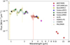
Fig. 8 SED of κ And b. The colored circles correspond to the IFS/spectrum data, while the colored pentagons are the photometric data. Note that we reduced the OSIRIS resolution spectrum to a low-resolution, IFS-like data (hereafter “OSIRIS-IFS”).
Uyama et al. 2020: They observed κ And with Subaru/SCExAO+HiCIAO using H- and Y-band broadband filters on 2016 July 18. The Y-band flux calibration was performed with HIP 118133 (6.60 ± 0.06 mag) and the H-band with HIP 79977 (7.85 ± 0.03 mag). The magnitudes of κ And and κ And b were determined to be 4.28 ± 0.09 and 17.04 ± 0.15 mag in the Y-band, and 15.18 ± 0.56 mag in the H-band for κ And b. Due to the larger uncertainties in the H-band, they excluded it from the atmospheric analysis. We decided not to use magnitude in the H-band for the same reason. Since the flux calibration was done using different stars (HIP 118133 for the Y-band), this measurement can be considered unbiased. As a check on our stellar spectrum, we calculated the magnitude in the Y-band of κ And, obtaining 4.25 ± 0.01 mag, consistent with Uyama et al. (2020, 4.28 ± 0.09 mag).
Figure 8 shows all the corrected data plus our JWST/MIRI observations. We note that all the datasets are consistent within 1–2σ.
4 Analysis and results
In this section we analyze the main properties of the companion κ And b. In Section 4.1, we qualitative describe the companion from the CMD from the MIRI filter CMD point of view. Then, in Section 4.2, we use two main families, cloudy and cloud-free, of atmospheric and evolutionary tracks models to infer the properties of κ And b. We first derive the age and mass by combining the MIRI CMD with isochrones. Then, by using atmospheric models, we fit the SED to obtain main physical parameters such as effective temperature and radius in Section 4.3. We combine these results with evolutionary tracks to derive the age and mass of the companion in Section 4.4. Finally, we used our age estimate to generate our MIRI sensitivity maps in Section 4.6.
4.1 MIRI color–magnitude diagram
Color-magnitude diagrams have long been essential for studying the atmospheric and physical properties of substellar objects across the M-to-Y spectral range (e.g., Kirkpatrick et al. 1999, Cushing et al. 2008). These diagrams provide a framework to disentangle the influence of effective temperature (Teff), surface gravity (log(g)), and atmospheric composition on the photometric and spectral properties of these objects. In the NIR (e.g., J–K vs. J, Fig. 1), M-type objects are dominated by water vapor and metal hydrides (red colors), while cooler T- and Y-dwarfs exhibit strong methane and ammonia absorption features displaying bluer colors (e.g., Leggett et al. 2010, Bonnefoy et al. 2013). MIRI/JWST F1065C-F1140C CMD reveal similar trends with greater sensitivity to condensates and minor species, enabling more precise differentiation between objects based on their atmospheric chemistry and thermal structure (e.g., Carter et al. 2023; Matthews et al. 2024; Mâlin et al. 2024; Godoy et al. 2024; Mâlin et al. 2025).
Figure 9 shows the F1065C–F1140C CMD, plotting with colored dots the field sources with different spectral types. The CMDs from left to right highlight (with marker sizes) the spectral index (from Suárez & Metchev 2022) related to the presence of different chemical species (methane, ammonia, and silicates, respectively). Figure 9 highlights the pivotal role of silicate and metal oxide clouds in early L-type atmospheres, especially for planetary-mass companions (Kirkpatrick 2005; Visscher et al. 2010; Morley et al. 2012; Morley et al. 2014). In these objects, Teff typically ranges from 1500 K to 2100 K, with surface gravities lower than those of field dwarfs due to their younger ages (Burgasser et al. 2002; Leggett et al. 2002). These differences result in thicker cloud decks and distinct molecular absorption features that set them apart from their field counterparts (e.g., Saumon & Marley 2008, Burgasser 2011). Early L dwarfs in particular serve as benchmarks for understanding the transition from cloud-dominated M-dwarfs to the clear atmospheres of T-dwarfs. Their location on the MIRI CMD is influenced by the presence of silicate clouds in the upper atmosphere, which gradually condense and disappear as the temperature drops, leaving behind clouds composed of different molecules and leading to a transition towards cloud-free atmospheres (e.g., Lodders & Fegley 2002; Zhang et al. 2018b; Zhang et al. 2018a; Suárez & Metchev 2022).
κ And b is situated at the top of the early L-type sequence in the F1065C–F1140C CMD (red star marker in Fig. 9), consistent with a Teff between 1600 K and 2000 K. This location suggests the presence of silicate clouds, consistent with its spectral classification of L0–L2 (e.g., Marley et al. 2002; Suárez & Metchev 2022). Compared to field sources, the younger age and lower surface gravity of the target imply a thicker, more optically active cloud layer (Allers & Liu 2013). Its position is notably distinct from that of other planetary-mass companions shown with gray diamonds in the CMD, which span a broader range of spectral types and Teff. The classification of our target as L0–L2 highlights its importance as a probe for understanding the early L-type sequence and its relation to the field and companion objects.
Although the CMD provides key insights into the atmospheric properties of the target, further progress requires a detailed MIR spectrum (e.g., Daemgen et al. 2017 for λ < 5 μm; Miles et al. 2023 covering the NIR to MIR). Such observations would allow for the precise identification of species like silicates and metal oxides, as well as an assessment of their concentration and vertical distribution in the κ And b atmosphere (e.g., Skemer et al. 2014). A spectrum would also enable robust comparisons between this target and other benchmark objects, advancing our understanding of the early L-type sequence and the broader context of planetary-mass companions in the MIR (e.g., Lodieu et al. 2018). Proven techniques for obtaining such spectra of high-contrast planets with JWST, in particular, using NIRSpec, have already been demonstrated (e.g., Ruffio et al. 2024), paving the way for similar analyzes of κ And b.
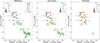 |
Fig. 9 CMD using the F1065C ad F1140C filters from MIRI. The dots correspond to the photometry obtained from the Spitzer spectra sample (Suárez & Metchev 2022), while the colors refer to the spectral type. The subplots correspond to the same CMD but show the methane (left), ammonia (middle), and silicates (right) spectral indices, as defined in Suárez & Metchev (2022), related to the depth of the absorption feature of each component. The circle sizes in each subplot refer to the value of the spectral index, as defined by Suárez & Metchev (2022). The gray dots in each panel correspond to species non-detection (i.e., plotted with index=0, not highlighted sources). The black dots refer to unclassified spectral types. The red star corresponds to κ And b, while the gray diamonds correspond to known planetary-mass companions (HR 2562 b from Godoy et al. 2024; VHS 1256 b from Miles et al. 2023; HD 95086 b from Mâlin et al. 2024; GJ 504 b from Mâlin et al. 2025; HR 8799 bcde from Boccaletti et al. 2024). The location and size of each planetary-mass companion are not related to the spectral index. Note that the Y-axis (i.e., MF1065C) refers to the absolute magnitude. Sample data taken from Godoy et al. (2024). |
4.2 Evolutionary tracks and color–magnitude diagram
When combined with theoretical evolutionary tracks, CMDs provide a robust method to derive key properties such as mass or age, directly from the photometric measurements, minimizing dependence on model fitting. This approach has been widely used in the literature to constrain the ages of stellar populations and substellar objects (e.g., Bonatto 2019), and giant planet companions such as AF Lep b (Gratton et al. 2024), and HIP 65426 b (Chauvin et al. 2017), enabling precise placement of objects on evolutionary grids and facilitating comparisons across a broad range of ages and masses.
For this analysis, we employed five evolutionary track models: ATMO chemical equilibrium (Phillips et al. 2020), AMES-COND (Allard et al. 2001), AMES-DUSTY (Chabrier et al. 2000), BT-Settl (Allard et al. 2012), and Sonora (Karalidi et al. 2021, Marley et al. 2021). These models span a range of atmospheric and cloud physics assumptions, which can display differences in the properties of substellar objects. To better understand the properties of κ And b, we used photometry in the H-band and the JWST/MIRI F1140C filter. The H-band is affected by cloud properties, changing the shape of the spectrum (e.g., Samland et al. 2017, Cheetham et al. 2019), while F1140C is affected by the presence of specific chemical species (e.g., Suárez & Metchev 2022, Mâlin et al. 2025). These bands cover key insights of the atmosphere properties, making these filters ideal to test different atmospheric models with different physics (cloudy and cloud-free properties).
To estimate the age and mass of κ And b for each evolutionary track, we calculated the compatibility between the observed photometry and each isochrone. Assuming Gaussian uncertainties for the magnitude and color of κ And b, we evaluated a score based on the proximity of the photometry to each isochrone in magnitude-color space. We first normalized the 2D Gaussian to have 1 at the maximum. Then, we evaluate each point of the isochrone in the Gaussian, obtaining a value in the range between 0 to 1, depending on the proximity to the Gaussian center. This score reflects the probability that the photometry for the object is consistent with a given isochrone. We associated masses from the isochrone with their respective scores for each age, constructing a probability-weighted distribution of masses and ages separately. Figure 10 presents the H-F1140C CMD, showing the isochrones spanning ages from 5 to 800 Myr for two evolution models (ATMO and Sonora). The colored circles represent field objects as described in Fig. 9.
We derived the most probable age and mass for κ And b for each evolutionary track. Since we also have the mass-age relation (each age associated with a score and mass), we calculated the age that corresponds to the derived mass (age as a function of mass). To ensure the robustness of our method, we validated it using VHS 1256b, a well-characterized benchmark object. A detailed description of the procedure and results for VHS 1256b is provided in Appendix F. The derived properties for κ And b are summarized in Table 6 for each evolutionary model and our final estimates for cloudy and cloud-free families. The cloud-free family has a final estimate in mass and age of 15.7 ± 2.3 MJup and 50 ± 8 Myr, while the cloudy family 18.1 ± 4.8 MJup and 50 ± 13 Myr, respectively. Both families align well with the ranges reported in the literature for the age (![Mathematical equation: $\[47_{-40}^{+27}\]$](/articles/aa/full_html/2025/10/aa54652-25/aa54652-25-eq20.png) Myr Jones et al. 2016) and mass (e.g.,
Myr Jones et al. 2016) and mass (e.g., ![Mathematical equation: $\[13_{-2}^{+12}\]$](/articles/aa/full_html/2025/10/aa54652-25/aa54652-25-eq21.png) MJup, Currie et al. 2018), further supporting the reliability of the derived parameters.
MJup, Currie et al. 2018), further supporting the reliability of the derived parameters.
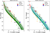 |
Fig. 10 CMD using H2MASS and F1140C. The blue pentagon corresponds to κ And b, while the red one to VHS 1256b (from Miles et al. 2023 and Godoy et al. 2024). The colored circles correspond to field sources shown in Fig. 9. Left: ATMO chemical equilibrium isochrones from 5 to 800 Myr, highlighting the 7 and 10 MJup for the isochrone of 5 Myr, also 25 and 35 MJup for the one of 800 Myr. Right: same as the left panel but for Sonora solar metallicity isochrones. |
Age and mass estimates for κ And b from the H-F1140C CMD and isochrones.
4.3 Atmospheric characterization of κ And b
Our MIRI measurements cover the Rayleigh-Jeans tail of the companion SED, providing for the first time a complete coverage of its bolometric emission. We thus started our analysis with a simple black body fit, which allows us to provide first-order constraints on its temperature and radius. Figure 11 shows the best-fit results in the dashed black line, and the range of Teff−radius and the respective χ2 values in color-scale lines. The best parameters are Teff=1795 ± 35 K, radius=1.30 ± 0.06 RJup, and log(L/L⊙)=−3.77 ± 0.07. These values are in agreement with the values in the literature (see Table 9). For these fits, we used a reduced number of photometric and synthetic photometric data points compared to the following more complex atmospheric model fits (see text below), but with adequate wavelength coverage to ensure a reliable fit. We also fit the black body excluding the MIRI data, obtaining a Teff=1949 ± 78 K, radius=1.21 ± 0.08 RJup, and log(L/L⊙)=−3.70 ± 0.06.
We then employed a variety of atmospheric models to gain a comprehensive understanding of the main characteristics of κ And b. These included ATMO in chemical equilibrium (ATMO-ceq, Phillips et al. 2020; Petrus et al. 2023), AMES-COND (Allard et al. 2001), AMES-DUSTY (Allard et al. 2001), BT-COND (Allard et al. 2012), BT-DUSTY (Allard et al. 2012), BT-Settl, DRIFT-PHOENIX (Helling et al. 2008), and EXO-REM (Charnay et al. 2018), configured for the cloudy (resolutions of 500 and 20 00011 and cloud-free (resolution of 500) conditions. Each model incorporates different physical assumptions and computational approaches, which are crucial to consider when comparing the best-fit results. Below, we briefly summarize the key features of each model.
The ATMO-ceq model simulates planetary atmospheres under the assumption of chemical equilibrium, where gas-phase abundances are determined by thermochemical equilibria without accounting for cloud formation. In contrast, EXOREM is a versatile model that accommodates the cloud-free and cloud-inclusive configurations, offering low- and high-resolution setups suitable for a range of exoplanetary environments. The AMES-COND and AMES-DUSTY models both focus on cloud formation but differ in their treatment of particulate matter: AMES-COND models cloud condensates, while AMES-DUSTY incorporates the role of dust grains, which significantly affect radiative transfer and energy balance. Similarly, BT-COND models atmospheric cloud condensates in radiative-convective equilibrium for brown dwarfs, while BT-DUSTY explicitly accounts for the scattering and absorption properties of dust particles. The BT-Settl model builds upon BT-COND by incorporating dynamic cloud-settling processes for a more realistic representation of cloud and dust behavior over time. Finally, PHOENIX, widely used for stellar and substellar objects, provides detailed radiative transfer calculations.
These models can be broadly categorized as cloud-free (ATMO-ceq, EXO-REM without clouds, BT-COND, AMES-COND) and cloudy (AMES-DUSTY, BT-DUSTY, BT-Settl, EXO-REM with clouds, and PHOENIX). From previous studies, we expect that the cloudy family fit better the SED of κ And b (e.g., Bonnefoy et al. 2014; Stone et al. 2020; Uyama et al. 2020).
We performed atmospheric fitting considering various data combinations and scenarios. Our dataset includes extensive NIR observations using different setups (narrow- and broad-band filters, IFS, and low- and medium-resolution spectra). These were grouped into different subsets to identify the best-fit models based on the lowest χ2 values. For the OSIRIS spectrum, we reduced the resolution to ~50 to have the same order of magnitude resolution as the other IFS data (R of ~20–70). The groups were all data combined, IFS + MIRI, photometry (NIR + MIR) alone, photometry (NIR + MIR) + synthetic photometry from IFS, IFS with priors from photometric (NIR + MIR) fitting, and IFS with priors from photometric (NIR + MIR) + synthetic photometry. Each atmospheric model was fitted to each data subset, resulting in 60 atmospheric fits. In addition, we did the same exercise, excluding the MIRI observations, to highlight the impact of the MIR data. We applied two critical considerations during the fitting process as listed below.
Wavelength weighting: Data were weighted across wavelengths to prevent biases due to regions with an over-density of observations in the NIR. This is, weighting by the number of observations in a given wavelength bin or band. Note that the standard fitting procedure assigns equal weight to all data points, ensuring that IFS observations do not carry more weight than photometric ones, but does not prevent over-density data in wavelength.
Parameter priors: Gaussian priors were applied to log(g) (N(4.5, 0.25)), effective temperature (N(1750, 350) K), and radius (N(1.4, 0.15), RJup). These priors were informed by results from the black body fit and ensured that solutions remained physically plausible and did not converge to the edge of the parameter grid.
We selected the best-fit models based on constraints requiring log(g) >3.9, radius >1.0 RJup, and temperatures >1650 K. We choose these restrictions based on previous estimates and on the L0/L2 spectral types properties. To account for known modeling biases due to post-processing choices (Nasedkin et al. 2023), we adopt a 1% systematic uncertainty on all parameters. This level is consistent with typical 1σ biases reported by Nasedkin et al. (2023), and ensures realistic error estimates, especially in cases where the fit fails to converge properly (e.g., underestimated errors in cloud-free models). The added uncertainty remains conservative without overcoming the formal statistical errors. Figure 12 shows the best-fit model for the data-subset with the best results for each atmospheric model considered. Cloudy models provided significantly better fits to the data, while cloud-free models exhibited larger discrepancies, particularly in the NIR. The EXO-REM model yielded the lowest χ2 values.
We note that when excluding MIRI observations, the model fitting converges, in general, to slightly higher effective temperatures, similar surface gravities, and smaller radii, regardless of the atmospheric family used. This suggests that without MIR constraints, models tend to over-estimate the effective temperature while compensating with lower radii to match the observed luminosity. Conversely, the MIRI data allow us to remove the degeneracy between these parameters. Regarding the improvement in uncertainties when using MIRI observations, we obtained for the cloud-free family an improvement of 6% for Teff, 2% for log(g), 6% for radius, and 3% for the spectroscopic mass, with no improvement for the luminosity. For the cloudy family, the improvements were 22% in Teff, 9% in log(g), 33% in radius, 1% in the spectroscopic mass, and 35% in luminosity.
We also tested including a circumplanetary blackbody disk component in the cloudy and cloud-free families fits. Cloud-free models are compatible with a disk flux contribution ranging from 0.2% to 35% across the MIRI bands, with flux-to-error ratios >30, yet still provide poor fits to the data. In contrast, cloudy models, especially the best-fit EXO-REM, indicate negligible disk contributions (<0.02%) with low significance (<1). Since the best-fitting models do not require a disk to explain the data, we conclude that any circumplanetary disk contribution is not statistically significant.
Table 7 shows the results for the cloudy and cloud-free models in terms of effective temperature, surface gravity, radius, spectroscopic mass, luminosity, and the respective χ2. We selected the data combination with the best ![Mathematical equation: $\[\chi_{\text {red }}^{2}\]$](/articles/aa/full_html/2025/10/aa54652-25/aa54652-25-eq22.png) . The table also shows the results without considering the MIRI data. We also calculated the weighted mean for the cloudy and cloud-free models for each parameter (fit including MIRI data) considering the natural dispersion in the uncertainties.
. The table also shows the results without considering the MIRI data. We also calculated the weighted mean for the cloudy and cloud-free models for each parameter (fit including MIRI data) considering the natural dispersion in the uncertainties.
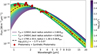 |
Fig. 11 SED of κ And b and the blackbody fitting results. The red circles correspond to observed photometry and calculated photometry from spectra observations (synthetic photometry). The colored lines correspond to the black body fit with temperatures from 1200 K to 2400 K (fixed) and the respective best-fit radius. The color gradient corresponds to the goodness-of-fit. The dashed black line corresponds to the best-fit model (temperature and radius as free parameters). |
4.4 Evolutionary tracks and physical parameters from atmospheric modeling
We used the results from atmospheric models combined with evolutionary tracks to assess whether the derived properties of κ And b align with theoretical predictions. Four evolutionary tracks were selected: ATMO-ceq, Saumon-2008 (Saumon & Marley 2008) Hybrid, Saumon-2008 No-Clouds, and Sonora solar metalicity (Marley et al. 2021). These models can be grouped into two families based on cloud treatment: cloudy (Saumon Hybrid and Sonora solar) and cloud-free (ATMO-ceq and Saumon No-Clouds). The atmospheric models were consistently paired with their respective evolutionary track families for analysis.
Using the effective temperature, surface gravity, and radius values listed in Table 7, we derived the mass and age of κ And b by interpolating within the evolutionary track grids. The interpolation was performed for three parameter combinations: Teff − log(g), Teff − radius, and radius − log(g). Figure 13 illustrates the evolutionary tracks for the ATMO-ceq and Sonora solar models, showing the grid combinations for Teff − radius and Teff − log(g).
We computed weighted averages of the derived mass and age values from the three-parameter grids for each evolutionary track family, using the χ2 values from the atmospheric model fits as weights. We also consider the natural dispersion of these measurements in the uncertainties. Table 8 presents the combined estimates for each evolutionary track and the final values for the cloudy and cloud-free families.
A key observation from Table 7 and Figure 13 is that log(g) exhibits larger uncertainties than Teff and radius, but this does not affect the uncertainties strongly because they are dominated by the data value dispersion in each grid (see Table 8). We adopted the mass and age estimates with the lowest uncertainties, corresponding to the Teff − log(g) grid, as our final results.
Interestingly, the comparison between cloudy and cloud-free models revealed similar trends. The cloud-free models predict slightly older ages (between 51 Myr and 60 Myr), while the cloudy models suggest younger ages (from 40 Myr to 56 Myr). The masses are similar and within the uncertainties. The precision of the cloudy family is better, however, which highlights the importance of the cloud treatment in atmospheric and evolutionary modeling for substellar companions such as κ And b.
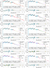 |
Fig. 12 Best-fit results from different atmospheric models. Each panel shows the best-fit model from a different combination of datasets, selected from all possible combinations. Each panel shows the photometric data (yellow pentagons), IFS (cyan circles), photometry from atmospheric model (magenta squares), and the best-fit model (colored line), and the residuals are shown in the bottom panel. Table 7 shows the data subset that corresponds to the best fit for each atmospheric model. |
Atmospheric and physical properties of κ And b.
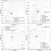 |
Fig. 13 Evolutionary tracks showing the age (continuum gray lines) and the mass (dashed dark gray lines) for a cloudy (Sonora with solar metallicity, right panels), and a cloud-free model (ATMO chemical equilibrium, left panels). Top: evolutionary tracks using the radius and effective temperature. Bottom: evolutionary tracks using effective temperature and log(g). The differently colored pentagons correspond to the values obtained from the atmospheric models. |
Age and mass estimates of κ And b using the evolutionary tracks and the atmospheric model fit results.
4.5 Final derived properties of κ And b
Table 9 presents the final estimates for the physical and atmospheric properties of κ And b, derived from a combination of CMDs with isochrones, atmospheric model fitting, and evolutionary tracks. We provide the results for the cloudy and cloud-free models, summarizing the findings into distinct categories for clarity. Additionally, we compare these estimates to values from the literature.
To offer a more comprehensive view, Figure 14 plots the derived, model-dependent age and mass from this study alongside literature values, highlighting the range of possible solutions and the convergence or divergence with previous studies. This summary provides a foundation for further discussion in Section 5, where we compare our findings with those of previous studies and discuss their implications for the formation and evolution of κ And b.
4.6 Mass limits and sensitivity
We used the synthetic stellar magnitudes for MIRI coronagraphic observations (see Table 2), the parallax of 19.406 ± 0.210 mas (Table 1), and an age of 47 ± 7 Myr from Table 9, combined with the contrast limits obtained in Section 3.3, to compute the sensitivity limits to additional companions, in Mass units.
We compared the detection limits with two evolutionary models: ATMO chemical equilibrium and AMES-DUSTY, a cloud-free and a cloudy model, respectively. Since the sensitivity magnitude for the F1550C data goes to faint sources outside of the DUSTY grid, we coupled it with the “Linder2019” (BEX models; Linder et al. 2019) evolutionary models (hereafter DUSTY-Linder2019). The Linder2019 models, in particular, account for the opacity and radiative effects of clouds, including their impact on atmospheric temperature gradients and emergent spectra. This makes them better suited for studying young or massive exoplanets, where cloud processes are significant. Figure 15 shows the sensitivity as a function of angular separation for the ATMO and DUSTY-Linder2019 models. The mass sensitivity is around 5 MJup above 4″ and below 10 MJup in the inner working angle region for both models.
We determined the sensitivity maps using the Exoplanet Detection Map Calculator (Exo-DMC12, Bonavita 2020) code. We followed the same approach described in Godoy et al. (2024) to compute the sensitivity map and propagate uncertainties, varying the mass between 0.1–110 MJup and the semi-major axis between 1 and 1200 AU. We simulated ~1.2 × 10⁸ orbits, with all the orbital parameters uniformly distributed, except for the eccentricity (see Bonavita 2020). Figures 16 and 17 present the results for the ATMO and DUSTY-Linder2019 mass limits.
The factor that most influences the uncertainty in the sensitivity map is age. By reducing the age uncertainties by a factor of ~3 with respect to the previous estimates (e.g., Jones et al. 2016), we better constrain the sensitivity. The reduced age uncertainty is reflected in the small deviation of masses in the sensitivity map (colored area in Figure 15, and dashed and dotted lines in Figures 16 and 17). The small differences between the predictions from ATMO and DUSTY-Linder2019 come from the relatively old age of 47 Myr, meaning an advanced atmospheric stage.
Our observations can detect, with 50% probability, objects with masses around 8 MJup at 40 AU (6.5 MJup at −1σ uncertainty) for both models. At 200 AU, the ATMO model has a sensitivity of 0.65 MJup (50% probability), while the DUSTY-Linder2019 model reaches 0.95 MJup, improving to 0.6 MJup and 0.67 MJup at 1σ, respectively. The semi-major axis of κ And b ranges between 55–125 AU (Uyama et al. 2020), and its clear detection in MIRI data implies a mass above 4 MJup, consistent with the literature and our measurements.
Atmospheric and physical properties of κ And b.
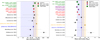 |
Fig. 14 Ages and masses estimated from literature and this work. Left: age estimates from the literature (black triangles), CMD plus isochrones (red pentagons), and evolutionary tracks plus atmospheric models (green squares). Right: mass estimates from the literature (black triangles), CMD plus isochrones (red pentagons), spectroscopic masses (purple diamond), and evolutionary tracks plus atmospheric models (green squares). For the estimates in this study, each method was sub-grouped into cloud and cloud-free models. The vertical dashed lines and filled area highlight the values obtained by Jones et al. (2016) using solar (blue) and subsolar (orange) metallicities. |
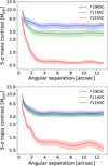 |
Fig. 15 Mass (from a 5σ sensitivity contrast) as a function of angular separation. Top: ATMO chemical equilibrium mass limits for F1065C, F1140C, and F1550C. Bottom: same as in the left panel but for DUSTY-Linder2009. |
5 Discussion
5.1 Physical parameters of κ And b
The large uncertainties in the age, the wide range of possible temperatures, and the model dependence in the derived mass, at the top of a nonuniform dataset, have generated discrepancies between past studies. The leverage provided by our long-wavelength observations has allowed us to contain the main properties of κ And b. Below we briefly discuss the implications of our new measurements on each parameter, and the meaning in the context of κ And b:
New age constraints: Age is perhaps the most important parameter for interpreting the physical characteristics of κ And b. It directly impacts mass, effective temperature, radius, and evolutionary state estimates, which in turn inform models of formation and atmospheric dynamics. The age of κ And b has been a source of significant controversy, however. Combining all the literature ages, the age ranges from 10 to 250 Myr (see Fig. 14), based on different techniques such as isochrone fitting (Bonnefoy et al. 2014), host stellar properties (Jones et al. 2016), or membership in moving groups (Hinkley et al. 2013; Bonnefoy et al. 2014).
Jones et al. (2016) derived an age of 47 Myr (+27/−40 Myr) based on interferometric observations and isochrone fitting using the inferred star properties, and this estimate has often been adopted as a reference. We employed two complementary methods based on the observations of the companion κ And b: CMD fitting with isochrones, and evolutionary track combined with atmospheric modeling. For the cloud-based atmospheric family, we derived a model-dependent age of 47 ± 7 Myr, perfectly consistent with Jones et al. (2016) and previous estimates but with an improvement in precision by a factor of ~4.8 and better uncertainty by ~79%. This reduced uncertainty represents an important advance and provides a better constraint for deriving other parameters such as mass.
Furthermore, our age estimate supports the membership of κ And b in the Columba moving group (Carson et al. 2013; Bonnefoy et al. 2014; Stone et al. 2020). Also, a well-constrained age enables better comparisons with other planetary-mass companions (e.g., those near to κ And b in the CMD; Figures 1 and 9), and more precise evolutionary history track, making κ And b a valuable benchmark for future atmospheric studies.
Mass estimates: The companion’s mass remains a key point of discussion. Estimates range from 13 MJup (Carson et al. 2013, Gratton et al. 2024) to nearly 50 MJup (Hinkley et al. 2013), depending on the assumed age and choice of evolutionary or atmospheric models (Fig. 14). Dynamical constraints (when available) provide the most robust mass estimates, especially when combining direct imaging with absolute astrometry (e.g., Snellen & Brown 2018; Brandt et al. 2019; Franson et al. 2022; Franson & Bowler 2023; Currie et al. 2023). The wide separation of κ And b (57–107 AU; Uyama et al. 2020) and the long orbital period limit the current effectiveness of this approach, however. Relative astrometry currently covers less than a decade and shows only linear motion, providing limited constraints on the orbit. Although no significant proper motion anomaly is seen in Gaia DR3, future analyzes combining longer-baseline astrometry and high-precision imaging, similar to those applied to β Pic b (Brandt et al. 2021) and HR 2562b (Zhang et al. 2023), may provide stronger dynamical constraints in the coming decades.
We derived two primary mass estimates: 17–19 MJup for the cloud-based family and 15–16 MJup for the cloud-free family. Given that the cloudy models better match the observed spectrum, the mass from this type of model is more likely accurate, so our best mass estimate from the overall spectroscopy is 17.3 ± 1.8 MJup, with errors bars smaller than previous estimates by 20%. This intermediate mass reconciles the long-standing debate between low-mass and high-mass solutions, situating κ And b in the transition between planets and brown dwarfs.
Notably, the mass estimate converges with values derived independently using three different methods (isochrones+CMD, atmospheric modeling, evolutionary tracks), all within the 1σ range: 18.1 ± 4.8, 17.3 ± 1.8, and 19 ± 2 MJup, respectively. This convergence underscores the robustness of our results and the impact of MIRI observations.
Effective temperature: The Teff of κ And b has been challenging to constrain due to its strong dependence on the assumed age, atmospheric models, and data used. Previous estimates ranged from 1650 K (Carson et al. 2013) to 2040 K (Hinkley et al. 2013). More recent studies (e.g., Uyama et al. 2020; Gratton et al. 2024) have suggested temperatures between 1700 K and 1850 K. It is important to note that the data used in each study may show discrepancies, either minor or significant, primarily due to differences in calibration procedures and in the stellar spectrum used to transform the contrast to absolute magnitude (see Section 3).
We find an effective temperature of 1791 ± 69 K using cloudy models, consistent with previous estimates and at similar precision (e.g., 69 K vs. 50 K, Stone et al. 2020). Cloud-free family yield similar averaged temperatures (1778 K). Our results highlight the importance of considering cloud-based physics when modeling such objects and the fitting procedure. Also, this temperature reflects well the position of κ And b in the CMD (see Figures 1 and 9), at the L0-L4 objects with high temperature and, qualitatively, low concentration of silicates.
We observe that the black body fits yield similar temperature results (1795 ± 35 K), highlighting the importance and impact of covering most (~90%) of the bolometric flux from substellar companions (from the NIR to the MIR). Even with a simple black body model, we can obtain a reliable estimate of the effective temperature of κ And b, showing the importance of MIRI in characterizing the atmosphere of substellar companions.
Radius: Previous radius estimates for κ And b were sparse and poorly constrained, with Wilcomb et al. (2020) suggesting 1.2 ± 0.3 RJup and Uyama et al. (2020) reporting 1.45 ± 0.15 RJup. Our analysis yields a more precise value of 1.42 ± 0.07 RJup, improving the precision by over 45%.
The cloud-free models predict a slightly reduced radius of 1.39 ± 0.04 RJup, consistent with the absence of prominent clouds and the need to compensate for slightly lower temperatures to match the observed luminosity. The radius from the cloud-free family is consistent with the radius from the cloudy family at 1σ, however. The gain of covering the NIR and MIR is that we can obtain a good estimate of the temperature and radius regardless of the atmospheric family we use. Again, the black body fit provides consistent results at 2σ level (1.30 ± 0.06 RJup), highlighting the importance of MIRI observations to constrain this parameter.
Surface gravity: The log(g) estimates in the literature have varied between 3.5 and 5.5 dex, with the most precise value being 4.75 ± 0.25 dex (Uyama et al. 2020). Our measurement of 4.35 ± 0.07 dex is notably lower but still within the 2σ range of previous estimates. This represents a ~70% improvement in precision.
The lower surface gravity has important implications for the classification of κ And b, supporting an L0–L2 spectral type (Uyama et al. 2020). A lower log(g) suggests a less compact atmosphere, which may influence cloud formation and atmospheric dynamics, and a younger age (e.g., log(g)=4.75 and 10–100 Myr, versus log(g)=4.35 and an age of 47 Mr). Our results highlight the need for medium- and high-resolution spectroscopy to refine and constrain the log(g) using the new constrained Teff as prior in the modeling.
Luminosity: Among the physical parameters of κ And b, luminosity estimates have shown minimal discrepancies across different studies. Previous estimates have ranged from log10(L/L⊙) = −3.76 to −3.81, with most values trending toward lower luminosities. The most precise measurement in the literature is −3.735 ± 0.045.
Our new measurement of −3.71 ± 0.07 is in agreement with previous estimates at the 2σ level, demonstrating the robustness of current models when incorporating new observational data. We note that the cloudy and cloud-free families have small differences, at the 1σ level (−3.76 ± 0.05 vs. −3.71 ± 0.07, respectively). As we mentioned before, the NIR observations coupled with MIRI cover most of the bolometric emission of κ And b, and this helps us to be less biased in the luminosity measurement. This is also reflected in the black body estimates (−3.77 ± 0.07), which are also in agreement with the cloudy, cloud-free families and literature.
The luminosity and age are key for studying the evolutionary pathway and dynamics of the atmosphere of exoplanets in direct imaging. These new constraints on the κ And b properties can help in further comparison with the directly imaged exoplanets and, in particular, with those reported in associations of similar ages such as the Tucana-Horologium Association (e.g., HR 8799 system). With the uncertainties of the main parameters of κ And b narrowed down, new studies related to the metallicity, chemical disequilibrium, presence of different species, and dust sedimentation will be keys to better understanding the atmospheric evolution of this companion and dynamic history of the κ And system.
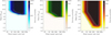 |
Fig. 16 Sensitivity of JWST/MIRI observations using the ATMO chemical equilibrium evolutionary track and an age of 47 ± 7 Myr. From left to right: F1065C, F1140C, and F1550C. The color bar in each plot means the detection probability, and the solid lines highlight the 10%, 50%, and 90% detection thresholds. The dotted and dashed lines correspond to 1σ uncertainties, respectively. |
5.2 Impact of variability
We emphasize the importance of a self-consistent calibration of all data in the analysis because this helps us to reduce bias sources. This recalibration does not eliminate other biases, however, such as internal calibration uncertainties or instrument performance variations. Another factor that we did not consider in our analysis is the potential variability due to a patchy atmosphere. Significant variability can impact atmospheric modeling, especially when combining datasets from different epochs, and it may vary across wavelengths. In addition, strong variability is very unlikely outside of the L to T transition (Radigan 2014).
We estimate the rotational period of κ And b using the projected rotational velocity v sin(i) = 38.42 ± 0.05 km/s from Morris et al. (2024) and our radius estimate of 1.42 ± 0.06 RJup. Morris et al. (2024) highlight that κ And b is a fast rotator, which suggests a short rotational period. We estimate the lower limit for the period to be P ≥ 4.61 ± 0.19 hours, slightly longer than the MIRI science target execution time of ~1.5 hours. In case of strong variability, the F1550C data would be the most impacted as it has the longest exposure time. The 11 years of observations, taken at different times and wavelengths, provide a broad temporal baseline that helps us to mitigate the impact of potential variability, if any. Since the data sample different epochs, the best-fit model effectively represents an average state of the source, with the residual dispersion naturally accounting for possible minor variations over time. To account for the impact of variability on the parameters, we have included 1% uncertainty in the retrieved parameters.
5.3 Brief comparison with other planetary-mass companions
κ And b lies in the L0–L4 spectral type range. This is a key phase for probing atmospheric processes in young self-luminous exoplanets. L-type companions offer insights into cloud formation, gravity effects, and thermal structure during early evolution. Comparable objects include β Picb (Lagrange et al. 2009), 2MASS J0219–3925 b (Artigau et al. 2015), and AB Pic b (Chauvin et al. 2005), all with ages between 21–37 Myr (Gratton et al. 2024), close to κ And b’s estimated age of ![Mathematical equation: $\[47_{-40}^{+27}\]$](/articles/aa/full_html/2025/10/aa54652-25/aa54652-25-eq178.png) Myr (Jones et al. 2016). These companions share similar atmospheric parameters: Teff ≈ 1680–1740 K, log(g) ≈ 4.2–4.5, and masses of 12–15, MJup. The close match to β Pic b particularly supports the derived values for κ And b (Teff ≈ 1790 K, log(g) ≈ 4.35, M ≈ 17 MJup), reinforcing its reliability and placing it among well-characterized young L-type companions.
Myr (Jones et al. 2016). These companions share similar atmospheric parameters: Teff ≈ 1680–1740 K, log(g) ≈ 4.2–4.5, and masses of 12–15, MJup. The close match to β Pic b particularly supports the derived values for κ And b (Teff ≈ 1790 K, log(g) ≈ 4.35, M ≈ 17 MJup), reinforcing its reliability and placing it among well-characterized young L-type companions.
Combining NIR and MIR data offers a more complete view of κ And b’s atmosphere. Our models indicate that cloudy atmospheres fit the spectrum better than cloud-free ones, consistent with condensate clouds inferred from high-resolution NIR spectra (Xuan et al. 2024). MIRI/MRS (Medium Resolution Spectroscopy) observations would enable direct detection of the 8–11 μm silicate absorption feature – seen in other L dwarfs (e.g., Cushing et al. 2006; Miles et al. 2023) – and provide deeper constraints on molecular abundances and the P–T structure. With its brightness and wide separation, κ And b is an ideal benchmark for studying cloud properties and atmospheric chemistry in young planetary-mass companions.
6 Summary and conclusions
We presented a refined characterization of the planetary-mass companion κ And b based on new JWST/MIRI observations in the F1065C, F1140C, and F1550C bandpasses. By combining MIR and NIR data, we captured most of the bolometric flux and significantly improved the constraints on the atmospheric parameters. Our analysis reduced the uncertainties in key properties such as effective temperature and radius and provided new estimates for the companion mass and age of the system. These improvements helped us to resolve a decade-long debate surrounding κ And b, whose inferred mass (13–50 MJup), surface gravity (3.5–5.5 dex), and effective temperature (1680–2050 K) have varied widely in the literature. The discrepancies were driven by inhomogeneous treatments of the observed dataset, the different atmospheric models that were used, and the large uncertainties in the age (10–250 Myr). Our study addressed these issues through a consistent reanalysis that offered a clearer picture of the nature of the companion.
Our first step was to recalibrate the archival data to have homogenous and consistent flux measurements of κ And b. To achieve this, we used the precise stellar parameters of κ And from Jones et al. (2016) to compute a stellar spectrum with a higher accuracy using the ATLAS/SYNTHE models. We conducted a study using four different methods to constrain the physical parameters of κ And b as listed below:
The MIRI CMD using the spectral index from Suárez & Metchev (2022) related to the presence of species in field brown dwarfs was used to understand the atmosphere stage and possible presence of specific species. From this comparison, we concluded that κ And b has a high temperature between 1600 K and 2000 K, with a possible small amount of silicates in the atmosphere. The presence of other species (methane, and ammonia) is completely ruled out because of the location of this companion in the CMD and the high-temperature restriction;
The combination of CMD with evolutionary tracks to derive the mass and age of the companion κ And b using the H and F1140C bands. We used two families of isochrones based on the physics used in the models: the cloudy family (AMES-DUSTY, BT-Settl, and Sonora solar metallicity), and the cloud-free family (AMES-COND and ATMO-ceq). We obtained an age and mass of 50 ± 8 Myr and 15.7 ± 2.3 MJup for the cloud-free family, and 50 ± 13 Myr and 18.1 ± 4.8 MJup for the cloudy family. This agrees with the values in the literature (e.g.,
![Mathematical equation: $\[13_{-2}^{+12}\]$](/articles/aa/full_html/2025/10/aa54652-25/aa54652-25-eq179.png) MJup, Currie et al. 2018, and
MJup, Currie et al. 2018, and ![Mathematical equation: $\[47_{-40}^{+27}\]$](/articles/aa/full_html/2025/10/aa54652-25/aa54652-25-eq180.png) Myr, Jones et al. 2016);
Myr, Jones et al. 2016);We modeled the atmosphere of κ And b using recalibrated archival data and new MIRI observations, and we tested cloudy (BT-DUSTY, BT-Settl, DRIFT-PHOENIX, and EXO-REM) and cloud-free (ATMO, AMES-COND, BT-COND, and EXO-REM no clouds) models. Physical priors and wavelength weighting were applied to ensure realistic solutions and to balance the NIR and MIR contributions. Cloudy models, especially EXO-REM, provided the best match to the full SED, while cloud-free models failed to reproduce the NIR spectrum. From the best fit, we derived a radius of 1.42 ± 0.06 RJup, a surface gravity of log(g)=4.35 ± 0.07 dex, and an effective temperature of 1791 ± 69 K. This improves the precision by ~22% for Teff and by ~33% for the radius compared to previous estimates;
We combined the atmospheric results with evolutionary tracks to constrain the age and mass of κ And b. We considered two model families: cloudy (Saumon2008 hybrid and Sonora solar metallicity) and cloud-free (ATMO and Saumon2008 no cloud) using the Teff, log(g), and radius solutions from all atmospheric models grouped accordingly. Since the cloudy models match the SED of κ And b best, we adopted them for our final estimate. The Teff–log(g) combination yields the smallest uncertainties and leads to an age of 47 ± 7 Myr and a mass of 17.3 ± 1.8 MJup.
With these results and analysis, we consider the following values as our final estimates of the physical parameters of κ And b: a spectroscopic mass of 17.3 ± 1.8 MJup, a Teff of 1791 ± 68 K, a radius of 1.42 ± 0.06 RJup, a surface gravity of 4.35 ± 0.07 dex, log10(L/L⊙) of −3.73 ± 0.02, and an age of 47 ± 7 Myr. These are all model-dependent estimates.
The MIRI observations have been key to obtaining precise measurements and improving the uncertainties of these parameters, especially in the effective temperature (22%) and radius (33%). This shows the impact of properly covering most of the bolometric flux of planetary-mass companions. Without MIRI data, all model classes were found to overestimate the effective temperatures and to underestimate the radii. The MIRI data allowed us to remove the degeneracy between these parameters, however. Our (model-dependent) age estimates of 47 ± 7 Myr agrees with the adopted age from Jones et al. (2016, ![Mathematical equation: $\[47_{-40}^{+27}\]$](/articles/aa/full_html/2025/10/aa54652-25/aa54652-25-eq181.png) Myr), but with significantly smaller uncertainties. This age is also consistent with the age of the Columba association (
Myr), but with significantly smaller uncertainties. This age is also consistent with the age of the Columba association (![Mathematical equation: $\[42_{-4}^{+6}\]$](/articles/aa/full_html/2025/10/aa54652-25/aa54652-25-eq182.png) Myr; Bell et al. 2015), which indicates that the κ And system might be a member of Columba, as previously suggested by Carson et al. (2013) and Bonnefoy et al. (2014). Our results lie in the middle range of the earlier measurements and also significantly reduce the error bars by 80%.
Myr; Bell et al. 2015), which indicates that the κ And system might be a member of Columba, as previously suggested by Carson et al. (2013) and Bonnefoy et al. (2014). Our results lie in the middle range of the earlier measurements and also significantly reduce the error bars by 80%.
We obtained a final value of 17.3 ± 1.8 MJup for the mass. This estimated value lies between the values reported in the literature. Consequently, κ And b is at the transition between giant planets and brown dwarfs. The Gaia mission, combined with new observations in the coming decades, will place strong constraints on the dynamical mass and help us to corroborate this estimate. The effective temperature and radius are consistent with the spectral classification (L0–L2; Uyama et al. 2020), suggesting a low abundance of certain metals and silicates in the atmosphere. The new constraints on age, mass, effective temperature, and radius will help us to understand the dynamical evolution of the system. Furthermore, while previous studies (e.g., Xuan et al. 2024; Wilcomb et al. 2020) have measured CO and H2O, constrained the C/O ratio, and retrieved a P–T profile for κ And b, the uncertainties remain large. New MIRI/MRS observations can confirm the presence of silicates, detect additional species, and refine our understanding of its atmospheric composition, cloud properties, and sedimentation state.
Data availability
The data used are available at the CDS via https://cdsarc.cds.unistra.fr/viz-bin/cat/J/A+A/702/A4.
Acknowledgements
This project is funded/Co-funded by the European Union (ERC, ESCAPE, project No. 101044152). Views and opinions expressed are however those of the author(s) only and do not necessarily reflect those of the European Union or the European Research Council Executive Agency. Neither the European Union nor the granting authority can be held responsible for them. These observations are associated with program #1241. This research has made use of computing facilities operated by CeSAM (Centre de données Astrophysiques de Marseille) data center at LAM (Laboratoire Astrophysique de Marseille), Marseille, France. We thank T. Stolker for providing support using the Species python package. We thank the authors Carson et al., Hinkley et al., Bonnefoy et al., Currie et al., Kuhn et al., Wilcomb et al., Stone et al., and Uyama et al., for providing and/or publishing the observational data used in this study. This work has made use of data from the European Space Agency (ESA) mission Gaia (https://www.cosmos.esa.int/gaia), processed by the Gaia Data Processing and Analysis Consortium (DPAC, https://www.cosmos.esa.int/web/gaia/dpac/consortium). Funding for the DPAC has been provided by national institutions, in particular, the institutions participating in the Gaia Multilateral Agreement. This research has made use of the Spanish Virtual Observatory (https://svo.cab.inta-csic.es) project funded by MCIN/AEI/10.13039/501100011033/ through grant PID2020-112949GB-I00. This publication makes use of VOSA, developed under the Spanish Virtual Observatory (https://svo.cab.inta-csic.es) project funded by MCIN/AEI/10.13039/501100011033/ through grant PID2020-112949GB-I00. VOSA has been partially updated by using funding from the European Union’s Horizon 2020 Research and Innovation Programme, under Grant Agreement No 776403 (EXOPLANETS-A). This publication makes use of data products from the Two Micron All Sky Survey, which is a joint project of the University of Massachusetts and the Infrared Processing and Analysis Center/California Institute of Technology, funded by the National Aeronautics and Space Administration and the National Science Foundation. This publication makes use of data products from the Wide-field Infrared Survey Explorer, which is a joint project of the University of California, Los Angeles, and the Jet Propulsion Laboratory/California Institute of Technology, funded by the National Aeronautics and Space Administration. This work has benefited from The UltracoolSheet, maintained by Will Best, Trent Dupuy, Michael Liu, Rob Siverd, and Zhoujian Zhang, and developed from compilations by Dupuy & Liu (2012, ApJS, 201, 19), Dupuy & Kraus (2013, Science, 341, 1492), Liu et al. (2016, ApJ, 833, 96), Best et al. (2018, ApJS, 234, 1), and Best et al. (2020b, AJ, in press). This research has made use of the Washington Double Star Catalog maintained at the U.S. Naval Observatory. M.M., A.B., P.-O.L. acknowledge funding support by CNES.
Appendix A Removing prominent and energetic cosmic rays
The pipeline spaceKLIP (which uses JWST pipeline routines) cannot remove some cosmic rays efficiently. For example, the most energetic cosmic rays are shown in the reduced frame on the left side in Figure 2. These energetic cosmic rays are challenging, and despite the initial parameters for the data reduction, they remain in the final image. Our approach is based on the nature of MIRI observations, which use nondestructive readout techniques (see Ressler et al. 2015), and works as a pre-reduction step at the raw data level. Essentially, the detector continuously collects data without interrupting the observation process or stopping the receipt of photons. As a result, the data consists of a series of images, each with progressively increasing flux measurements. From the perspective of a single pixel, this process resembles a ramp, where the slope of the ramp represents the increase in detected signal over time.
When a cosmic ray strikes a pixel, it causes a sudden increase in the signal, appearing as a sharp jump in the ramp (Anderson & Gordon 2011). This jump is distinct from the steady increase caused by incoming photons and can be detected and corrected during data processing. Figure A.1 shows one pixel centered at three cosmic rays received at different times in dashed, colored lines. The image shows the “jump” in the so-called digital units (flux measurement unit in the detector). The correction used by the pipeline works well for low-energy cosmic rays but results in more masked pixels and residual structures with higher-energy ones. Our procedure breaks the ramp into individual images, generating a series of exposures. As a result, a cosmic ray impact will be captured in one of these images, corresponding to the moment of the cosmic-ray arrival. Figure A.2 presents three consecutive images of the same three pixels shown in Figure A.1. The middle image contains the cosmic ray, which is absent in the subsequent image. Figure A.3 shows the signal of these three single-pixels across the image series (flux difference between each consecutive pair of groups within the ramp). The cosmic ray appears as an outlier in the curves.
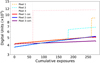 |
Fig. A.1 Ramp in one integration for MIRI observations at F1550C filter for three specific pixels. The dotted colored lines are the original ramp for three pixels at the location of three different cosmic rays that impacted at different times during the integration. The solid-colored lines are the corrected ramp for these three pixels. |
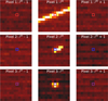 |
Fig. A.2 Images showing the ramp separated into individual integrations and ordered in time, centered at the cosmic ray hit (middle column). The first and third columns are the moments before and after the hit of the cosmic ray. The colored squares in each panel highlight the pixel selected in Figure A.1 for each cosmic ray (different rows). The images have the same color scale. |
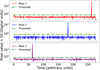 |
Fig. A.3 Flux difference between consecutive groups for each selected pixel affected by a cosmic ray. The red, blue, and purple curves correspond to each pixel flux as a function of time. The dashed green line corresponds to the threshold used to select outliers. The cosmic ray hit appears as a peak in each flux-differentiation ramp. |
By analyzing the differentiated-ramp flux across all images, we can create a representative image by computing the median to avoid outlier effects. The outliers can be identified using a threshold of six times the MAD (green dashed line in Figure A.3) and then replaced with the median value. This method effectively identifies high-energy cosmic rays but may miss low-energy ones and bad pixels, as they do not produce significant variations in the differentiated ramp. We then restore the ramp structure using the corrected differentiated ramp flux. Figure A.1 shows the ramp before (dashed colored lines) and after (solid colored lines) cosmic ray removal, while Figure A.4 shows the last image in the ramp before (left) and after (right) cosmic ray correction.
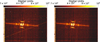 |
Fig. A.4 Second row ramp integration of the third dither position of the reference star HD 222389 at F1550C filter. Left: Raw, last image in the ramp integration without applying any correction (raw or *uncal* image). Right: Same frame but applying the cosmic rays and basic bad pixel corrections directly in the raw image. |
Appendix B Fringing structure*
The fringing structure is present in the reference star integrations in the F1065C and F1140C filters. The fringing directly impacts post-processing, resulting in poor (or even no) correction of the coronagraphic stellar PSF in the science target. Figure B.1 shows this effect in the PCA subtraction in κ And at F1065C using 15 components. We proceed as follows to remove and correct the fringing in all the reference integrations. To exemplify the procedure, we show here the first integration of the first dither position of the reference star at F1065C. First, we identify the main structure by computing the median value in the X (along the columns) and Y (along the rows) axes. Figure B.2 shows the values per column (top) and rows (bottom) and the respective median (red curve) values. The fringing structure is visible on the bottom side. We also noted the dispersion along both axes, which reached a mean upper value of 100 MJy/str.
We proceed as follows to correct this structure presented in all the reference star integrations in F1065C and F1140C filters:
1) We computed the median Nj0 along the Y-axis (median of each row) in the image Ii,j. Then we compute the median level n0 of Nj.
2) We calculated, per column Ii, the corrected image ![Mathematical equation: $\[I_{i}^{\prime}\]$](/articles/aa/full_html/2025/10/aa54652-25/aa54652-25-eq183.png) using the following equation
using the following equation ![Mathematical equation: $\[I_{i}^{\prime}=I_{i}-N_{j}+n_{0}\]$](/articles/aa/full_html/2025/10/aa54652-25/aa54652-25-eq184.png) .
.
3) We repeated steps 1) and 2) two more times using the resulting I′ as input each time to obtain a final I″. Figure B.3 shows the resulting image at the top and the Y-axis structure at the bottom. Figure B.4 shows the same as Figure B.2 but now using the corrected image I″. We note that we still have remnant fringing structures that were not corrected using the previous steps in both figures. Since we still have these remnant fringing structures at the left and right sides of the image, we proceed to fix them individually.
4) We computed the MAD Mi along the X-axis. The MAD values will be higher when we still have the presence of the fringing structure and minimum in the regions where we successfully removed the fringing in the previous steps.
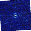 |
Fig. B.1 Post-processing, PCA subtraction of κ And using RDI and 15 components. In this case, the reference frames were not corrected for the fringing structure. |
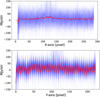 |
Fig. B.2 Main structures and flux dispersion in the X and Y axes. Top: Median value along the x-axis corresponds to the median value per column. Bottom: Same but for the y-axis, and along the rows. The blue lines correspond to the values per column (left) and row (right), while the red line corresponds to the respective median. |
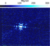 |
Fig. B.3 Resulting image after the first iterations to correct the fringing structure. The remnant fringing is still present on the left and right sides of the image. |
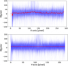 |
Fig. B.4 Same as Figure B.2 but now using the first fringing corrections. |
5) To identify the significant remnant fringing structure (i.e., above the noise level), we fit a polynomial of degree 2, Pi, to get the main structure in Mi. Then, we normalized Mi using Pi. We used the normalized Mi to compute the standard deviation, which represents the main noise level and out cutoff level. Figure B.5 shows Mi, Pi, and the cutoff level.
6) We calculated the intersection between the fit model Pi and the cutoff level. This defines the left and right regions still affected by the fringing structure.
7) We repeated steps 1) and 2) but now used the left and right areas separately. Figure B.6 shows the point 4) after applying the correction to each region. Figures B.7 show the image Ii,j after the correction on the left (top) and right (bottom) regions, separately.
8) Finally, we corrected the most prominent negative outliers in the image using the routine cube_correct_nan from the VIP python package and σ-clipping with σ = 5 and five iterations.
Figure B.9 shows the main structure in the X and Y axes as in Figure B.2. Figure B.8 shows the same as Figure B.5 but after applying the fringing corrections in the left and right regions. We note that the fringing structure disappeared, and the noise level was reduced from ~100 to ~60 MJy/sr. Figure 3 shows the image before and after applying these corrections.
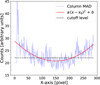 |
Fig. B.5 MAD along the columns of the first fringing corrections applied to the image (transparent blue curve). The red curve corresponds to the fitted polynomial Pi, and the dashed black line to the cutoff level. |
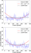 |
Fig. B.6 Same as Figure B.5 but after applying the fringing corrections. Top: Corrections applied only to the left region in step 6). Bottom: Correction applied only to the right region. |
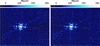 |
Fig. B.7 Image after the first and second fringing corrections for the left (left) and right (right) regions. |
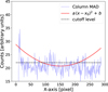 |
Fig. B.8 Same as Figure B.5 but using the image after all the fringing corrections. |
 |
Fig. B.9 Same as Figure B.2 but after applying all the fringing corrections. |
Appendix C Best extraction parameters
To determine the flux and astrometric position of κ And b with minimal uncertainty and bias, we conducted several tests using different numbers of principal components in post-processing. These components were crucial for effectively removing the coronagraphic PSF and speckles, which in turn impacted the signal, flux measurement, and astrometric accuracy of the companion. We utilized the fake planet injection method from spaceKLIP across 1 to 15 components and calculated the S/N with VIP. Additionally, we assessed the post-extraction residuals, flux, magnitude, and relative position in pixels. Since the companion has a low signal, we evaluate the option to blur (to smooth) the integrations. We perform the same analysis with smoothed and unsmoothed frames. Figures C.2 and C.1 show these values as a function of the number of components subtracted for each of the three filters.
The optimal results are summarized in Table C.1 for unsmoothed and smoothed frames. These selections were based on the highest S/N, stable relative position, consistent flux values with low uncertainty, and minimized r.m.s., indicating efficient starlight removal. The differences between the two approaches are within the uncertainties, but the case of the smoothed frame has better-extracted parameters in terms of r.m.s. and uncertainties. The best number of components are 10, 7, and 8 for the F1065C, F1140C, and F1550C filters, respectively.
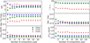 |
Fig. C.1 General extraction quality for κ And b without smoothing the frames. Left-top: Signal-to-noise ratio as a function of the number of components used (NPC). Left-middle: Apparent flux vs. NPC. Left-bottom: Relative position (with respect to the coronagraph) along the X-axis vs. NPC (in pixels). Right-top: Root-mean-square in the residual image after subtracting the companion vs. NPC. Right-middle: Apparent magnitude in Vega system vs. NPC. Right-bottom: Relative position along the Y-axis vs. NPC (in pixels). Blue circles, red triangles, and green diamonds correspond to the bandpasses F1065C, F1140C, and F1550C, respectively. Vertical gray lines are the uncertainties. |
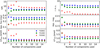 |
Fig. C.2 Same as Figure C.1 but smoothing the frames. |
Best extraction parameters for the unsmoothed and smoothed data for κ And b.
Appendix D Bad-pixel effects in companion extraction
We note the presence of persistent hot pixels at the location of κ And b in the F1550C filter. These pixels may or may not bias the measurements of the flux and astrometry of κ And b. To investigate this possibility, we injected a fake planet at the same separation as κ And b on the opposite side of the companion (i.e., at PA+~180°). The fake planet was injected using a simulated PSF and renormalized to approximately match the flux of κ And b. We individually injected the same bad and hot pixels in the residuals (see Fig. 5). Then, we proceeded with the post-processing and companion extraction as done for κ And b. We repeated the same procedure without injecting the bad and hot pixels to compare the flux extraction results. Figure D.1 shows the extracted flux for the case without (red) and with (blue) bad pixels. We found that the injected fake planet with bad pixels has ~6% (~0.09 × 10⁻⁴) more flux than the one without bad pixels. Because the uncertainties are larger (~0.28 × 10⁻⁴), however, the contribution of this 6% difference can be considered within the actual uncertainties: 0.29 × 10⁻⁴ vs. 0.28 × 10⁻⁴. We determine that the bad and hot pixels within the κ And b PSF are not biasing the measured flux of the companion.
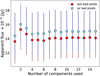 |
Fig. D.1 Flux measured from the PSF modeling of an injected fake planet at the same angular separation but at a position angle shifted by ~180° relative to κ And b. The red dots represent the flux extraction of the injected fake planet without any bad or hot pixels. The light blue dots correspond to the same fake planet but include bad and hot pixels. The vertical line in each colored point corresponds to the uncertainty. |
Appendix E Archival data correction
We compute our stellar spectrum model using ATLAS/SYNTHE models based on the physical parameters derived by Jones et al. (2016). We collected all the archival data and used stellar model. We used the stellar model from the literature and our model to compute a corrector factor in all the datasets.
The correction is more notorious in spectroscopic observations since we are able to see the changes in the shape of the companion spectrum. We first reduced the resolution of the two stellar model spectra to the resolution of the IFS/medium-resolution observation. Then, we divided them to compute a corrector factor as a function of wavelength. These values are then directly multiplied in the IFS/medium-resolution observations of the companion κ And b. Figure E.1 shows the comparison between our stellar models and those used by Currie et al. (2018) and Stone et al. (2020). Figure E.2 shows on the left the stellar models of our ATLAS and the B9V Pickles library model used by Hinkley et al. (2013), and on the right, the ratio of the two models at the resolution of the IFS observation.
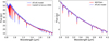 |
Fig. E.1 Stellar model spectrum used in this study (blue line) and the model used by Currie et al. (2018) in the left panel, and by Stone et al. (2020) in the right panel (red line). |
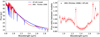 |
Fig. E.2 Synthetic stellar spectrum (blue line) and the B9V Pickles library spectrum (red line) used to convert the companion contrast into flux (Hinkley et al. 2013). Left: Two stellar model spectra in the wavelength range of the IFS observation. Right: Ratio of the two model spectra at the resolution of the IFS observation. This ratio corresponds to the corrector factor. |
We corrected all the spectra observations of κ And b following the procedure describe above. Figure E.3 shows all the archival spectroscopic data of κ And b (black dots and lines), and our correction using our ATLAS stellar model spectrum (red dots and lines) for (from top to bottom):Hinkley et al. (2013), Currie et al. (2018), Stone et al. (2020), and Wilcomb et al. (2020).
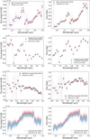 |
Fig. E.3 κ And b archival spectroscopic data (light blue dots) and corrected data (red dots). The left panels show the flux in erg/cm2/s/A, while the right panels shows the flux in mJy. |
Appendix F Age and mass estimates from CMD+isochrones
We employed our method to estimate the mass and age from the CMD plus isochrones, of the VHS 1256 b companion. How was mentioned before, each isochrone has an associated score and a representative mass. This comes from the evaluation of the isochrone in the 2D Gaussian profile, normalized to 1 at the maximum. The 2D Gaussian corresponds to the photometric measurement of the companion, i.e., the color and absolute magnitude, and related uncertainties. For each isochrone, we evaluated the mass track into the 2D Gaussian, whose values can range from 0 to 1. This is equivalent to estimating how good the color-match of a specific mass is in the isochrone with respect to our companion fluxes. When the isochrone matches perfectly the color–magnitude of the companion, the score is 1, while the score will be zero if the isochrone completely mismatches it. Then, for each isochrone, we have a mass distribution (score vs. mass), for which we can estimate the representative mass and the dispersion as uncertainty. This mass is calculated using a weighted mean, with the weight being the associated score for each mass. We kept the maximum score associated with each isochrone to make the age versus score and mass versus score distribution. This distribution in mass corresponds to the weighted mean mass for each isochrone and the best evaluated score. The final age and mass estimates were calculated using the weighted mean and a score threshold of 0.6. Figures F.1 and F.2 show the mass and age (x-axis) with the respective score (y-axis) for the AMES-COND and Sonora-solar isochrones, respectively. The probable mass and age from the distributions were presented at the top of each figure.
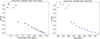 |
Fig. F.1 Distribution of mass and age for VHS 1256 b using AMES-COND evolutionary tracks. Left: Best score and probable mass for each isochrone. The masses (x-axis) were sorted from younger to older associated age from the isochrone. The error bar corresponds to the mass-dispersion measurement in each isochrone. Right: Isochronal age and the best evaluated score. The final values for each parameter (mass and age) are presented at the top of each figure. |
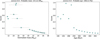 |
Fig. F.2 Same as Figure F.1 but using Sonora solar metallicity evolutionary tracks. |
Figure F.3 shows the age as a function of mass with the respective associated score in color for the two evolutionary tracks. We calculated the probable age from the most probable mass and uncertainty via Monte Carlo (i.e., age as a function of mass-age(mass)). At the top of each figure, we show the two probable ages and masses. From AMES-COND we estimated an age(mass) of 164 ± 16 Myr and mass of 12.5 ± 1.3 MJup, while for Sonora-solar we obtained an age(mass) of 176 ± 59 Myr and 14.1 ± 2.3 MJup, respectively. Dupuy et al. (2023) reported an age for VHS 1256 of 140 ± 20 Myr and a companion mass between 12 MJup and 16 MJup. Our age and mass estimates are in agreement with the one reported by Dupuy et al. (2023) at 1σ level, further supporting our procedure to derive those parameters for κ And b. Notoriously, in Figure F.3 (more clearly in the left panel), we observe a double peak in the mass axis, which is in agreement with the bi-modal distribution of mass reported by Miles et al. (2023, Fig. 10), with both peaks at ~12MJup and ~16MJup.
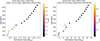 |
Fig. F.3 Age as a function of the most probable mass using AMES-COND (left) and Sonora-solar (right) evolutionary tracks. The color-scale corresponds to the associated score. The final calculated values for age and mass are presented at the top of each figure. |
References
- Allard, F., Hauschildt, P. H., Alexander, D. R., Tamanai, A., & Schweitzer, A. 2001, ApJ, 556, 357 [Google Scholar]
- Allard, F., Homeier, D., & Freytag, B. 2012, Philos. Trans. Roy. Soc. Lond. A, 370, 2765 [NASA ADS] [Google Scholar]
- Allers, K. N., & Liu, M. C. 2013, ApJ, 772, 79 [NASA ADS] [CrossRef] [Google Scholar]
- Anderson, R. E., & Gordon, K. D. 2011, PASP, 123, 1237 [NASA ADS] [CrossRef] [Google Scholar]
- Artigau, É., Gagné, J., Faherty, J., et al. 2015, ApJ, 806, 254 [NASA ADS] [CrossRef] [Google Scholar]
- Beichman, C. A., Neugebauer, G., Habing, H. J., Clegg, P. E., & Chester, T. J., eds. 1988, Infrared Astronomical Satellite (IRAS) Catalogs and Atlases: Explanatory Supplement, 1 [Google Scholar]
- Bell, C. P. M., Mamajek, E. E., & Naylor, T. 2015, MNRAS, 454, 593 [Google Scholar]
- Best, W. M. J., Dupuy, T. J., Liu, M. C., Siverd, R. J., & Zhang, Z. 2021, https://doi.org/10.5281/zenodo.4570814 [Google Scholar]
- Boccaletti, A., Lagage, P. O., Baudoz, P., et al. 2015, PASP, 127, 633 [CrossRef] [Google Scholar]
- Boccaletti, A., Cossou, C., Baudoz, P., et al. 2022, A&A, 667, A165 [NASA ADS] [CrossRef] [EDP Sciences] [Google Scholar]
- Boccaletti, A., Mâlin, M., Baudoz, P., et al. 2024, A&A, 686, A33 [NASA ADS] [CrossRef] [EDP Sciences] [Google Scholar]
- Bonatto, C. 2019, MNRAS, 483, 2758 [NASA ADS] [CrossRef] [Google Scholar]
- Bonavita, M. 2020, Exo-DMC: Exoplanet Detection Map Calculator, Astrophysics Source Code Library [record ascl:2010.008] [Google Scholar]
- Bonnefoy, M., Boccaletti, A., Lagrange, A. M., et al. 2013, A&A, 555, A107 [NASA ADS] [CrossRef] [EDP Sciences] [Google Scholar]
- Bonnefoy, M., Currie, T., Marleau, G. D., et al. 2014, A&A, 562, A111 [NASA ADS] [CrossRef] [EDP Sciences] [Google Scholar]
- Bowler, B. P. 2016, PASP, 128, 102001 [Google Scholar]
- Brandt, T. D., Dupuy, T. J., & Bowler, B. P. 2019, AJ, 158, 140 [Google Scholar]
- Brandt, G. M., Brandt, T. D., Dupuy, T. J., Li, Y., & Michalik, D. 2021, AJ, 161, 179 [NASA ADS] [CrossRef] [Google Scholar]
- Burgasser, A. J. 2011, in Astronomical Society of the Pacific Conference Series, 450, Molecules in the Atmospheres of Extrasolar Planets, eds. J. P. Beaulieu, S. Dieters, & G. Tinetti, 113 [Google Scholar]
- Burgasser, A. J., Kirkpatrick, J. D., Brown, M. E., et al. 2002, ApJ, 564, 421 [NASA ADS] [CrossRef] [Google Scholar]
- Burggraaff, O., Talens, G. J. J., Spronck, J., et al. 2018, A&A, 617, A32 [NASA ADS] [CrossRef] [EDP Sciences] [Google Scholar]
- Burrows, C. J., Krist, J. E., Stapelfeldt, K. R., & WFPC2 Investigation Definition Team. 1995, in American Astronomical Society Meeting Abstracts, 187, 32.05 [Google Scholar]
- Burrows, A., Sudarsky, D., & Hubeny, I. 2006, ApJ, 640, 1063 [Google Scholar]
- Bushouse, H., Eisenhamer, J., Dencheva, N., et al. 2022, https://doi.org/10.5281/zenodo.6984366 [Google Scholar]
- Cannon, A. J., & Pickering, E. C. 1993, VizieR Online Data Catalog: Henry Draper Catalogue and Extension (Cannon+ 1918–1924; ADC 1989), VizieR On-line Data Catalog: III/135A. Originally published in: Harv. Ann. 91–100 (1918–1924) [Google Scholar]
- Carson, J., Thalmann, C., Janson, M., et al. 2013, ApJ, 763, L32 [Google Scholar]
- Carter, A. L., Hinkley, S., Kammerer, J., et al. 2023, ApJ, 951, L20 [NASA ADS] [CrossRef] [Google Scholar]
- Castelli, F., & Kurucz, R. L. 2003, in IAU Symposium, 210, Modelling of Stellar Atmospheres, eds. N. Piskunov, W. W. Weiss, & D. F. Gray, A20 [Google Scholar]
- Chabrier, G., Baraffe, I., Allard, F., & Hauschildt, P. 2000, ApJ, 542, 464 [Google Scholar]
- Charnay, B., Bézard, B., Baudino, J. L., et al. 2018, ApJ, 854, 172 [Google Scholar]
- Chauvin, G., Lagrange, A. M., Zuckerman, B., et al. 2005, A&A, 438, L29 [NASA ADS] [CrossRef] [EDP Sciences] [Google Scholar]
- Chauvin, G., Desidera, S., Lagrange, A. M., et al. 2017, A&A, 605, L9 [NASA ADS] [CrossRef] [EDP Sciences] [Google Scholar]
- Cheetham, A. C., Samland, M., Brems, S. S., et al. 2019, A&A, 622, A80 [NASA ADS] [CrossRef] [EDP Sciences] [Google Scholar]
- Clemens, D. P., Sarcia, D., Grabau, A., et al. 2007, PASP, 119, 1385 [NASA ADS] [CrossRef] [Google Scholar]
- Couture, D., Gagné, J., & Doyon, R. 2023, ApJ, 946, 6 [NASA ADS] [CrossRef] [Google Scholar]
- Currie, T., Burrows, A., Itoh, Y., et al. 2011, ApJ, 729, 128 [Google Scholar]
- Currie, T., Brandt, T. D., Uyama, T., et al. 2018, AJ, 156, 291 [Google Scholar]
- Currie, T., Brandt, G. M., Brandt, T. D., et al. 2023, Science, 380, 198 [NASA ADS] [CrossRef] [Google Scholar]
- Cushing, M. C., Rayner, J. T., & Vacca, W. D. 2005, ApJ, 623, 1115 [Google Scholar]
- Cushing, M. C., Roellig, T. L., Marley, M. S., et al. 2006, ApJ, 648, 614 [Google Scholar]
- Cushing, M. C., Marley, M. S., Saumon, D., et al. 2008, ApJ, 678, 1372 [NASA ADS] [CrossRef] [Google Scholar]
- Daemgen, S., Todorov, K., Silva, J., et al. 2017, A&A, 601, A65 [NASA ADS] [CrossRef] [EDP Sciences] [Google Scholar]
- Danielski, C., Baudino, J.-L., Lagage, P.-O., et al. 2018, AJ, 156, 276 [Google Scholar]
- De Rosa, R. J., Rameau, J., Patience, J., et al. 2016, ApJ, 824, 121 [Google Scholar]
- Ducati, J. R. 2002, VizieR Online Data Catalog: Catalogue of Stellar Photometry in Johnson’s 11-color system., CDS/ADC Collection of Electronic Catalogues, 2237, 0 [Google Scholar]
- Dupuy, T. J., Liu, M. C., Evans, E. L., et al. 2023, MNRAS, 519, 1688 [Google Scholar]
- Fortney, J. J., Marley, M. S., Saumon, D., & Lodders, K. 2008, ApJ, 683, 1104 [Google Scholar]
- Franson, K., & Bowler, B. P. 2023, AJ, 165, 246 [NASA ADS] [CrossRef] [Google Scholar]
- Franson, K., Bowler, B. P., Brandt, T. D., et al. 2022, AJ, 163, 50 [NASA ADS] [CrossRef] [Google Scholar]
- Gaia Collaboration (Prusti, T., et al.) 2016, A&A, 595, A1 [NASA ADS] [CrossRef] [EDP Sciences] [Google Scholar]
- Gaia Collaboration 2020, VizieR Online Data Catalog: I/350 [Google Scholar]
- Garrison, R. F., & Gray, R. O. 1994, AJ, 107, 1556 [NASA ADS] [CrossRef] [Google Scholar]
- Godoy, N., Choquet, E., Serabyn, E., et al. 2024, A&A, 689, A185 [NASA ADS] [CrossRef] [EDP Sciences] [Google Scholar]
- Gratton, R., Bonavita, M., Mesa, D., et al. 2024, A&A, 684, A69 [NASA ADS] [CrossRef] [EDP Sciences] [Google Scholar]
- Groff, T. D., Kasdin, N. J., Limbach, M. A., et al. 2014, SPIE Conf. Ser., 9147, 91471W [NASA ADS] [Google Scholar]
- Groff, T. D., Kasdin, N. J., Limbach, M. A., et al. 2015, SPIE Conf. Ser., 9605, 96051C [NASA ADS] [Google Scholar]
- Hauschildt, P. H., Allard, F., Ferguson, J., Baron, E., & Alexander, D. R. 1999, ApJ, 525, 871 [Google Scholar]
- Helling, C., Dehn, M., Woitke, P., & Hauschildt, P. H. 2008, ApJ, 675, L105 [NASA ADS] [CrossRef] [Google Scholar]
- Helou, G., & Walker, D. W. 1988, Infrared Astronomical Satellite (IRAS) Catalogs and Atlases, 7: The Small Scale Structure Catalog [Google Scholar]
- Hinkley, S., Oppenheimer, B. R., Brenner, D., et al. 2008, SPIE Conf. Ser., 7015, 701519 [Google Scholar]
- Hinkley, S., Oppenheimer, B. R., Zimmerman, N., et al. 2011, PASP, 123, 74 [CrossRef] [Google Scholar]
- Hinkley, S., Pueyo, L., Faherty, J. K., et al. 2013, ApJ, 779, 153 [NASA ADS] [CrossRef] [Google Scholar]
- HIP 1997, ESA Special Publication, 1200, The HIPPARCOS and TYCHO catalogues. Astrometric and photometric star catalogues derived from the ESA HIPPARCOS Space Astrometry Mission [Google Scholar]
- Hodapp, K. W., Suzuki, R., Tamura, M., et al. 2008, SPIE Conf. Ser., 7014, 701419 [Google Scholar]
- Høg, E., Fabricius, C., Makarov, V. V., et al. 2000, A&A, 357, 367 [NASA ADS] [Google Scholar]
- Ishihara, D., Onaka, T., Kataza, H., et al. 2010, A&A, 514, A1 [NASA ADS] [CrossRef] [EDP Sciences] [Google Scholar]
- Jones, J., White, R. J., Quinn, S., et al. 2016, ApJ, 822, L3 [Google Scholar]
- Kammerer, J., Girard, J., Carter, A. L., et al. 2022, SPIE Conf. Ser., 12180, 121803N [Google Scholar]
- Karalidi, T., Marley, M., Fortney, J. J., et al. 2021, ApJ, 923, 269 [NASA ADS] [CrossRef] [Google Scholar]
- Kirkpatrick, J. D. 2005, ARA&A, 43, 195 [NASA ADS] [CrossRef] [Google Scholar]
- Kirkpatrick, J. D., Reid, I. N., Liebert, J., et al. 1999, ApJ, 519, 802 [NASA ADS] [CrossRef] [Google Scholar]
- Kühn, J., Serabyn, E., Lozi, J., et al. 2018, PASP, 130, 035001 [Google Scholar]
- Kurucz, R. L. 2013, ATLAS12: Opacity sampling model atmosphere program, Astrophysics Source Code Library [record ascl:1303.024] [Google Scholar]
- Kurucz, R. L. 2014, in Determination of Atmospheric Parameters of B, eds. E. Niemczura, B. Smalley, & W. Pych, 39 [Google Scholar]
- Lagrange, A. M., Gratadour, D., Chauvin, G., et al. 2009, A&A, 493, L21 [NASA ADS] [CrossRef] [EDP Sciences] [Google Scholar]
- Lagrange, A. M., Bonnefoy, M., Chauvin, G., et al. 2010, Science, 329, 57 [Google Scholar]
- Lajoie, C.-P., Soummer, R., Pueyo, L., et al. 2016, SPIE Conf. Ser., 9904, 99045K [NASA ADS] [Google Scholar]
- Larkin, J., Barczys, M., Krabbe, A., et al. 2006, New A Rev., 50, 362 [CrossRef] [Google Scholar]
- Lebzelter, T., Mowlavi, N., Lecoeur-Taibi, I., et al. 2023, A&A, 674, A15 [NASA ADS] [CrossRef] [EDP Sciences] [Google Scholar]
- Leggett, S. K., Golimowski, D. A., Fan, X., et al. 2002, ApJ, 564, 452 [Google Scholar]
- Leggett, S. K., Burningham, B., Saumon, D., et al. 2010, ApJ, 710, 1627 [Google Scholar]
- Linder, E. F., Mordasini, C., Mollière, P., et al. 2019, A&A, 623, A85 [NASA ADS] [CrossRef] [EDP Sciences] [Google Scholar]
- Lodders, K., & Fegley, B. 2002, Icarus, 155, 393 [Google Scholar]
- Lodieu, N., Zapatero Osorio, M. R., Béjar, V. J. S., & Peña Ramírez, K. 2018, MNRAS, 473, 2020 [Google Scholar]
- Mâlin, M., Boccaletti, A., Perrot, C., et al. 2025, A&A, 693, A315 [NASA ADS] [CrossRef] [EDP Sciences] [Google Scholar]
- Mâlin, M., Boccaletti, A., Perrot, C., et al. 2024, A&A, 690, A316 [NASA ADS] [CrossRef] [EDP Sciences] [Google Scholar]
- Marleau, G. D., & Cumming, A. 2014, MNRAS, 437, 1378 [Google Scholar]
- Marley, M. S., Seager, S., Saumon, D., et al. 2002, ApJ, 568, 335 [NASA ADS] [CrossRef] [Google Scholar]
- Marley, M. S., Saumon, D., Cushing, M., et al. 2012, ApJ, 754, 135 [Google Scholar]
- Marley, M. S., Saumon, D., Visscher, C., et al. 2021, ApJ, 920, 85 [NASA ADS] [CrossRef] [Google Scholar]
- Marois, C., Macintosh, B., Barman, T., et al. 2008, Science, 322, 1348 [Google Scholar]
- Matthews, E. C., Carter, A. L., Pathak, P., et al. 2024, Nature, 633, 789 [NASA ADS] [CrossRef] [Google Scholar]
- Mawet, D., Milli, J., Wahhaj, Z., et al. 2014, ApJ, 792, 97 [Google Scholar]
- Mermilliod, J. C. 1997, VizieR Online Data Catalog: Homogeneous Means in the UBV System (Mermilliod 1991), VizieR On-line Data Catalog: II/168. Originally published in: Institut d’Astronomie, Universite de Lausanne (1991) [Google Scholar]
- Mesa, D., Baudino, J. L., Charnay, B., et al. 2018, A&A, 612, A92 [NASA ADS] [CrossRef] [EDP Sciences] [Google Scholar]
- Miles, B. E., Biller, B. A., Patapis, P., et al. 2023, ApJ, 946, L6 [NASA ADS] [CrossRef] [Google Scholar]
- Morley, C. V., Fortney, J. J., Marley, M. S., et al. 2012, ApJ, 756, 172 [NASA ADS] [CrossRef] [Google Scholar]
- Morley, C. V., Marley, M. S., Fortney, J. J., & Lupu, R. 2014, ApJ, 789, L14 [NASA ADS] [CrossRef] [Google Scholar]
- Morris, E. C., Wang, J. J., Hsu, C.-C., et al. 2024, AJ, 168, 144 [NASA ADS] [Google Scholar]
- Murakami, H., Baba, H., Barthel, P., et al. 2007, PASJ, 59, S369 [CrossRef] [Google Scholar]
- Nasa / Esa / Serc 2004, VizieR Online Data Catalog: Final Merged Log of IUE Observations (NASA-ESA, 2000), VizieR On-line Data Catalog: VI/110. Originally published in: IUE Newsletters (1978–2000) [Google Scholar]
- Nasedkin, E., Mollière, P., Wang, J., et al. 2023, A&A, 678, A41 [NASA ADS] [CrossRef] [EDP Sciences] [Google Scholar]
- Nielsen, E. L., De Rosa, R. J., Macintosh, B., et al. 2019, AJ, 158, 13 [Google Scholar]
- Öberg, K. I., Murray-Clay, R., & Bergin, E. A. 2011, ApJ, 743, L16 [Google Scholar]
- Ochsenbein, F., Bauer, P., & Marcout, J. 2000, A&AS, 143, 23 [NASA ADS] [CrossRef] [EDP Sciences] [Google Scholar]
- Onaka, T., Matsuhara, H., Wada, T., et al. 2007, PASJ, 59, S401 [Google Scholar]
- Oppenheimer, B. R., Beichman, C., Brenner, D., et al. 2012, SPIE Conf. Ser., 8447, 844720 [Google Scholar]
- Paunzen, E. 2015, A&A, 580, A23 [NASA ADS] [CrossRef] [EDP Sciences] [Google Scholar]
- Peters-Limbach, M. A., Groff, T., Kasdin, N. J., et al. 2012, SPIE Conf. Ser., 8446, 84467U [Google Scholar]
- Petrus, S., Chauvin, G., Bonnefoy, M., et al. 2023, A&A, 670, L9 [NASA ADS] [CrossRef] [EDP Sciences] [Google Scholar]
- Phillips, M. W., Tremblin, P., Baraffe, I., et al. 2020, A&A, 637, A38 [NASA ADS] [CrossRef] [EDP Sciences] [Google Scholar]
- Pickles, A. J. 1998, PASP, 110, 863 [NASA ADS] [CrossRef] [Google Scholar]
- Radigan, J. 2014, ApJ, 797, 120 [NASA ADS] [CrossRef] [Google Scholar]
- Rajan, A., Rameau, J., De Rosa, R. J., et al. 2017, AJ, 154, 10 [Google Scholar]
- Ressler, M. E., Sukhatme, K. G., Franklin, B. R., et al. 2015, PASP, 127, 675 [CrossRef] [Google Scholar]
- Rieke, G. H., Ressler, M. E., Morrison, J. E., et al. 2015, PASP, 127, 665 [NASA ADS] [CrossRef] [Google Scholar]
- Rigby, J., Perrin, M., McElwain, M., et al. 2023, PASP, 135, 048001 [NASA ADS] [CrossRef] [Google Scholar]
- Rodrigo, C., & Solano, E. 2020, in XIV.0 Scientific Meeting (virtual) of the Spanish Astronomical Society, 182 [Google Scholar]
- Rodrigo, C., Solano, E., & Bayo, A. 2012, SVO Filter Profile Service Version 1.0, IVOA Working Draft 15 October 2012 [Google Scholar]
- Rouan, D., Riaud, P., Boccaletti, A., Clénet, Y., & Labeyrie, A. 2000, PASP, 112, 1479 [Google Scholar]
- Ruffio, J.-B., Perrin, M. D., Hoch, K. K. W., et al. 2024, AJ, 168, 73 [NASA ADS] [CrossRef] [Google Scholar]
- Samland, M., Mollière, P., Bonnefoy, M., et al. 2017, A&A, 603, A57 [NASA ADS] [CrossRef] [EDP Sciences] [Google Scholar]
- Saumon, D., & Marley, M. S. 2008, ApJ, 689, 1327 [Google Scholar]
- Skemer, A. J., Marley, M. S., Hinz, P. M., et al. 2014, ApJ, 792, 17 [Google Scholar]
- Smith, B. A., & Terrile, R. J. 1984, Science, 226, 1421 [Google Scholar]
- Snellen, I. A. G., & Brown, A. G. A. 2018, Nat. Astron., 2, 883 [Google Scholar]
- Spiegel, D. S., & Burrows, A. 2012, ApJ, 745, 174 [Google Scholar]
- Stone, J. M., Barman, T., Skemer, A. J., et al. 2020, AJ, 160, 262 [Google Scholar]
- Suárez, G., & Metchev, S. 2022, MNRAS, 513, 5701 [CrossRef] [Google Scholar]
- Sutlieff, B. J., Bohn, A. J., Birkby, J. L., et al. 2021, MNRAS, 506, 3224 [NASA ADS] [CrossRef] [Google Scholar]
- Todorov, K. O., Line, M. R., Pineda, J. E., et al. 2016, ApJ, 823, 14 [CrossRef] [Google Scholar]
- Tokunaga, A. T., Kobayashi, N., Bell, J., et al. 1998, SPIE Conf. Ser., 3354, 512 [Google Scholar]
- Tremblin, P., Amundsen, D. S., Chabrier, G., et al. 2016, ApJ, 817, L19 [NASA ADS] [CrossRef] [Google Scholar]
- Uyama, T., Currie, T., Hori, Y., et al. 2020, AJ, 159, 40 [Google Scholar]
- Vigan, A., Fontanive, C., Meyer, M., et al. 2021, A&A, 651, A72 [EDP Sciences] [Google Scholar]
- Visscher, C., Lodders, K., & Fegley, Jr., B. 2010, ApJ, 716, 1060 [NASA ADS] [CrossRef] [Google Scholar]
- Wilcomb, K. K., Konopacky, Q. M., Barman, T. S., et al. 2020, AJ, 160, 207 [Google Scholar]
- Wright, E. L., Eisenhardt, P. R. M., Mainzer, A. K., et al. 2010, AJ, 140, 1868 [Google Scholar]
- Wright, G. S., Wright, D., Goodson, G. B., et al. 2015, PASP, 127, 595 [NASA ADS] [CrossRef] [Google Scholar]
- Xuan, W. J., Mawet, D., Ngo, H., et al. 2018, AJ, 156, 156 [NASA ADS] [CrossRef] [Google Scholar]
- Xuan, J. W., Wang, J., Ruffio, J.-B., et al. 2022, ApJ, 937, 54 [NASA ADS] [CrossRef] [Google Scholar]
- Xuan, J. W., Hsu, C.-C., Finnerty, L., et al. 2024, ApJ, 970, 71 [CrossRef] [Google Scholar]
- Zhang, Z. H., Galvez-Ortiz, M. C., Pinfield, D. J., et al. 2018a, MNRAS, 480, 5447 [NASA ADS] [CrossRef] [Google Scholar]
- Zhang, Z. H., Pinfield, D. J., Gálvez-Ortiz, M. C., et al. 2018b, MNRAS, 479, 1383 [NASA ADS] [CrossRef] [Google Scholar]
- Zhang, S. Y., Duchêne, G., De Rosa, R. J., et al. 2023, AJ, 165, 219 [Google Scholar]
- Zuckerman, B., Rhee, J. H., Song, I., & Bessell, M. S. 2011, ApJ, 732, 61 [Google Scholar]
We used a microturbulence of 2 km/s.
We adopted a metalicity equal to zero, as Jones et al. (2016).
WIYN: Wisconsin-Indiana-Yale-NOIRLab. WHIRC: WIYN High-Resolution Infrared Camera.
The differences between NEXGEN models with Teff = 10 000 K, log(g) values of 4.0 and 4.5 dex, and different metallicities are minor compared to our ATLAS spectrum and within uncertainties.
Although generated with the same code and parameters, the two EXO-REM cloudy models show small intrinsic differences (~0.2%) before and after resolution degradation, possibly due to differences in the numerical processes requiring more or less detailed atmospheric modeling.
Since we processed the data, this “fringing” has been associated with the 390 Hz pattern noise seen in many MIRI subarray observations. The effect is described at https://jwst-docs.stsci.edu/known-issues-with-jwst-data/miri-known-issues#MIRIKnownIssues-emiElectromagneticinterference(EMI)patternnoise. A pipeline correction is now available as part of the emicorr step of the calwebb_detector1 module of the pipeline.
All Tables
Photometry and astrometry of κ And b derived from the MIRI coronagraphic observations.
Corrected magnitudes archival data of κ And b using κ And ATLAS atmospheric model.
Age and mass estimates of κ And b using the evolutionary tracks and the atmospheric model fit results.
All Figures
|
Fig. 1 CMD showing the position of κ And b (red hexagon marker) relative to the population of low-mass stars and brown dwarfs (colored circles) as obtained from Best et al. (2021). The different colors highlight the different spectral types. The gray pentagons correspond to selected directly imaged planets (DIP) and planetary-mass companions (PMCs). |
| In the text | |
|
Fig. 2 Second integration of the third dither position of the reference star HD 222389 after the BACKGROUND subtraction at the F1550C filter. Left: Frame with the standard data reduction parameters using spaceKLIP. Right: same frame, but directly applying our cosmic-ray and bad-pixel corrections in the raw frame. |
| In the text | |
|
Fig. 3 First integration of the third dither position of the reference star HD 222389 after the background subtraction at the F1065C filter. Left: frame with the fringing structure (horizontal lines) after applying the normal reduction. Right: same frame after applying our additional correction procedure, in which we removed the fringing structure. |
| In the text | |
|
Fig. 4 Top: SED of the star κ Andromedae. The orange dots correspond to the photometric data from Table 2. Red dots correspond to our synthetic photometry using the F1065C, F1140C, and F1550C bandpasses. The blue line corresponds to the mean between the 1000 realizations of ATLAS models with the respective uncertainties. Bottom: Residuals between the model and the data. The gray region corresponds to 3σ. |
| In the text | |
|
Fig. 5 Modeling and extraction of the companion κ And b. From top to bottom: filters F1065C, F1140C, and F1550C. Left: post-processed science images, corresponding to 10,7, and 8 components for the filters F1065C, F1140C, and F1550C, respectively. Middle: best spaceKLIP model of the companion using webb_psf. Right: residuals after subtracting the model from the science data. The field of view corresponds to 25 × 25 pixels (~2.75″ × 2.75″). The images in each row have the same color scale. The gray region with white lines represents a hatched mask corresponding to the star behind the coronagraph. |
| In the text | |
|
Fig. 6 Pre- and post-processing frames of κ And. Top: background-subtracted and stacked science frames. The stacking is only for visualization purposes. Bottom: starlight-subtracted image using RDI and KLIP at the optimal number of components. From left to right: F1065C, F1140C, and F1550C filters. The horizontal white arrow highlights the position of κ And b. Each of the columns (i.e., filters) has the same color scale. The yellow star in each subplot marks the position of the star κ And. North is up and east to the left. |
| In the text | |
|
Fig. 7 Smoothed contrast limits for all JWST/MIRI κ And observations in the F1065C (blue), F1140C (green), and F1550C (red) bandpasses. |
| In the text | |
|
Fig. 8 SED of κ And b. The colored circles correspond to the IFS/spectrum data, while the colored pentagons are the photometric data. Note that we reduced the OSIRIS resolution spectrum to a low-resolution, IFS-like data (hereafter “OSIRIS-IFS”). |
| In the text | |
|
Fig. 9 CMD using the F1065C ad F1140C filters from MIRI. The dots correspond to the photometry obtained from the Spitzer spectra sample (Suárez & Metchev 2022), while the colors refer to the spectral type. The subplots correspond to the same CMD but show the methane (left), ammonia (middle), and silicates (right) spectral indices, as defined in Suárez & Metchev (2022), related to the depth of the absorption feature of each component. The circle sizes in each subplot refer to the value of the spectral index, as defined by Suárez & Metchev (2022). The gray dots in each panel correspond to species non-detection (i.e., plotted with index=0, not highlighted sources). The black dots refer to unclassified spectral types. The red star corresponds to κ And b, while the gray diamonds correspond to known planetary-mass companions (HR 2562 b from Godoy et al. 2024; VHS 1256 b from Miles et al. 2023; HD 95086 b from Mâlin et al. 2024; GJ 504 b from Mâlin et al. 2025; HR 8799 bcde from Boccaletti et al. 2024). The location and size of each planetary-mass companion are not related to the spectral index. Note that the Y-axis (i.e., MF1065C) refers to the absolute magnitude. Sample data taken from Godoy et al. (2024). |
| In the text | |
|
Fig. 10 CMD using H2MASS and F1140C. The blue pentagon corresponds to κ And b, while the red one to VHS 1256b (from Miles et al. 2023 and Godoy et al. 2024). The colored circles correspond to field sources shown in Fig. 9. Left: ATMO chemical equilibrium isochrones from 5 to 800 Myr, highlighting the 7 and 10 MJup for the isochrone of 5 Myr, also 25 and 35 MJup for the one of 800 Myr. Right: same as the left panel but for Sonora solar metallicity isochrones. |
| In the text | |
|
Fig. 11 SED of κ And b and the blackbody fitting results. The red circles correspond to observed photometry and calculated photometry from spectra observations (synthetic photometry). The colored lines correspond to the black body fit with temperatures from 1200 K to 2400 K (fixed) and the respective best-fit radius. The color gradient corresponds to the goodness-of-fit. The dashed black line corresponds to the best-fit model (temperature and radius as free parameters). |
| In the text | |
|
Fig. 12 Best-fit results from different atmospheric models. Each panel shows the best-fit model from a different combination of datasets, selected from all possible combinations. Each panel shows the photometric data (yellow pentagons), IFS (cyan circles), photometry from atmospheric model (magenta squares), and the best-fit model (colored line), and the residuals are shown in the bottom panel. Table 7 shows the data subset that corresponds to the best fit for each atmospheric model. |
| In the text | |
|
Fig. 13 Evolutionary tracks showing the age (continuum gray lines) and the mass (dashed dark gray lines) for a cloudy (Sonora with solar metallicity, right panels), and a cloud-free model (ATMO chemical equilibrium, left panels). Top: evolutionary tracks using the radius and effective temperature. Bottom: evolutionary tracks using effective temperature and log(g). The differently colored pentagons correspond to the values obtained from the atmospheric models. |
| In the text | |
|
Fig. 14 Ages and masses estimated from literature and this work. Left: age estimates from the literature (black triangles), CMD plus isochrones (red pentagons), and evolutionary tracks plus atmospheric models (green squares). Right: mass estimates from the literature (black triangles), CMD plus isochrones (red pentagons), spectroscopic masses (purple diamond), and evolutionary tracks plus atmospheric models (green squares). For the estimates in this study, each method was sub-grouped into cloud and cloud-free models. The vertical dashed lines and filled area highlight the values obtained by Jones et al. (2016) using solar (blue) and subsolar (orange) metallicities. |
| In the text | |
|
Fig. 15 Mass (from a 5σ sensitivity contrast) as a function of angular separation. Top: ATMO chemical equilibrium mass limits for F1065C, F1140C, and F1550C. Bottom: same as in the left panel but for DUSTY-Linder2009. |
| In the text | |
|
Fig. 16 Sensitivity of JWST/MIRI observations using the ATMO chemical equilibrium evolutionary track and an age of 47 ± 7 Myr. From left to right: F1065C, F1140C, and F1550C. The color bar in each plot means the detection probability, and the solid lines highlight the 10%, 50%, and 90% detection thresholds. The dotted and dashed lines correspond to 1σ uncertainties, respectively. |
| In the text | |
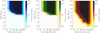 |
Fig. 17 Same as Figure 16 but using the DUSTY-Linder2009 evolutionary tracks. |
| In the text | |
|
Fig. A.1 Ramp in one integration for MIRI observations at F1550C filter for three specific pixels. The dotted colored lines are the original ramp for three pixels at the location of three different cosmic rays that impacted at different times during the integration. The solid-colored lines are the corrected ramp for these three pixels. |
| In the text | |
|
Fig. A.2 Images showing the ramp separated into individual integrations and ordered in time, centered at the cosmic ray hit (middle column). The first and third columns are the moments before and after the hit of the cosmic ray. The colored squares in each panel highlight the pixel selected in Figure A.1 for each cosmic ray (different rows). The images have the same color scale. |
| In the text | |
|
Fig. A.3 Flux difference between consecutive groups for each selected pixel affected by a cosmic ray. The red, blue, and purple curves correspond to each pixel flux as a function of time. The dashed green line corresponds to the threshold used to select outliers. The cosmic ray hit appears as a peak in each flux-differentiation ramp. |
| In the text | |
|
Fig. A.4 Second row ramp integration of the third dither position of the reference star HD 222389 at F1550C filter. Left: Raw, last image in the ramp integration without applying any correction (raw or *uncal* image). Right: Same frame but applying the cosmic rays and basic bad pixel corrections directly in the raw image. |
| In the text | |
|
Fig. B.1 Post-processing, PCA subtraction of κ And using RDI and 15 components. In this case, the reference frames were not corrected for the fringing structure. |
| In the text | |
|
Fig. B.2 Main structures and flux dispersion in the X and Y axes. Top: Median value along the x-axis corresponds to the median value per column. Bottom: Same but for the y-axis, and along the rows. The blue lines correspond to the values per column (left) and row (right), while the red line corresponds to the respective median. |
| In the text | |
|
Fig. B.3 Resulting image after the first iterations to correct the fringing structure. The remnant fringing is still present on the left and right sides of the image. |
| In the text | |
|
Fig. B.4 Same as Figure B.2 but now using the first fringing corrections. |
| In the text | |
|
Fig. B.5 MAD along the columns of the first fringing corrections applied to the image (transparent blue curve). The red curve corresponds to the fitted polynomial Pi, and the dashed black line to the cutoff level. |
| In the text | |
|
Fig. B.6 Same as Figure B.5 but after applying the fringing corrections. Top: Corrections applied only to the left region in step 6). Bottom: Correction applied only to the right region. |
| In the text | |
|
Fig. B.7 Image after the first and second fringing corrections for the left (left) and right (right) regions. |
| In the text | |
|
Fig. B.8 Same as Figure B.5 but using the image after all the fringing corrections. |
| In the text | |
|
Fig. B.9 Same as Figure B.2 but after applying all the fringing corrections. |
| In the text | |
|
Fig. C.1 General extraction quality for κ And b without smoothing the frames. Left-top: Signal-to-noise ratio as a function of the number of components used (NPC). Left-middle: Apparent flux vs. NPC. Left-bottom: Relative position (with respect to the coronagraph) along the X-axis vs. NPC (in pixels). Right-top: Root-mean-square in the residual image after subtracting the companion vs. NPC. Right-middle: Apparent magnitude in Vega system vs. NPC. Right-bottom: Relative position along the Y-axis vs. NPC (in pixels). Blue circles, red triangles, and green diamonds correspond to the bandpasses F1065C, F1140C, and F1550C, respectively. Vertical gray lines are the uncertainties. |
| In the text | |
|
Fig. C.2 Same as Figure C.1 but smoothing the frames. |
| In the text | |
|
Fig. D.1 Flux measured from the PSF modeling of an injected fake planet at the same angular separation but at a position angle shifted by ~180° relative to κ And b. The red dots represent the flux extraction of the injected fake planet without any bad or hot pixels. The light blue dots correspond to the same fake planet but include bad and hot pixels. The vertical line in each colored point corresponds to the uncertainty. |
| In the text | |
|
Fig. E.1 Stellar model spectrum used in this study (blue line) and the model used by Currie et al. (2018) in the left panel, and by Stone et al. (2020) in the right panel (red line). |
| In the text | |
|
Fig. E.2 Synthetic stellar spectrum (blue line) and the B9V Pickles library spectrum (red line) used to convert the companion contrast into flux (Hinkley et al. 2013). Left: Two stellar model spectra in the wavelength range of the IFS observation. Right: Ratio of the two model spectra at the resolution of the IFS observation. This ratio corresponds to the corrector factor. |
| In the text | |
|
Fig. E.3 κ And b archival spectroscopic data (light blue dots) and corrected data (red dots). The left panels show the flux in erg/cm2/s/A, while the right panels shows the flux in mJy. |
| In the text | |
|
Fig. F.1 Distribution of mass and age for VHS 1256 b using AMES-COND evolutionary tracks. Left: Best score and probable mass for each isochrone. The masses (x-axis) were sorted from younger to older associated age from the isochrone. The error bar corresponds to the mass-dispersion measurement in each isochrone. Right: Isochronal age and the best evaluated score. The final values for each parameter (mass and age) are presented at the top of each figure. |
| In the text | |
|
Fig. F.2 Same as Figure F.1 but using Sonora solar metallicity evolutionary tracks. |
| In the text | |
|
Fig. F.3 Age as a function of the most probable mass using AMES-COND (left) and Sonora-solar (right) evolutionary tracks. The color-scale corresponds to the associated score. The final calculated values for age and mass are presented at the top of each figure. |
| In the text | |
Current usage metrics show cumulative count of Article Views (full-text article views including HTML views, PDF and ePub downloads, according to the available data) and Abstracts Views on Vision4Press platform.
Data correspond to usage on the plateform after 2015. The current usage metrics is available 48-96 hours after online publication and is updated daily on week days.
Initial download of the metrics may take a while.