| Issue |
A&A
Volume 702, October 2025
|
|
|---|---|---|
| Article Number | A235 | |
| Number of page(s) | 20 | |
| Section | Stellar structure and evolution | |
| DOI | https://doi.org/10.1051/0004-6361/202555704 | |
| Published online | 24 October 2025 | |
The stellar evolution perspective on the metallicity dependence of classical Cepheid Leavitt laws
1
Institute of Physics, École Polytechnique Fédérale de Lausanne (EPFL), Observatoire de Sauverny, 1290 Versoix, Switzerland
2
Department of Astronomy, University of Geneva, Chemin Pegasi 51b, 1290 Versoix, Switzerland
3
European Space Agency (ESA), ESA Office, Space Telescope Science Institute, 3700 San Martin Drive, Baltimore, MD 21218, USA
⋆ Corresponding authors: This email address is being protected from spambots. You need JavaScript enabled to view it.
; This email address is being protected from spambots. You need JavaScript enabled to view it.
Received:
28
May
2025
Accepted:
6
August
2025
Abstract
Metallicity is a key parameter in stellar evolution and it significantly affects measurements of the mass-luminosity relation of classical Cepheids (henceforth, Cepheids). The impact of metallicity on the Cepheid Leavitt law (period-luminosity relation; henceforth, LL) and, in turn, the Hubble constant (H0), has been the subject of much recent debate. While recent observational results have generally shown a negative intercept-metallicity effect at all wavelengths and for Wesenheit magnitudes, predictions based on different stellar evolution models have differed even in terms of sign. Here, we present a comprehensive analysis of metallicity effects on Cepheid LLs based on synthetic Cepheid populations computed using Geneva stellar evolution models and the SYCLIST tool. We computed 296 co-eval populations in the age range of 5 − 300 Myr for metallicities representative of the Sun, the LMC, and the SMC (Z ∈ [0.014, 0.006, 0.002]). We computed LLs in fourteen optical-to-infrared passbands spanning from GaiaGBP to JWST’s F444W and five reddening-free Wesenheit magnitudes. All Cepheid populations take into account distributions of rotation rates and companion stars. We found an excellent agreement between the predicted populations and key observational constraints from the literature, such as a) instability strip (IS) boundaries, b) period distributions, c) LL slopes, and d) intrinsic LL dispersion as a function of wavelength and metallicity (match within 0.01 mag). This is further strengthened by the previously demonstrated excellent agreement between the same models and observed mass-luminosity relations, period-radius relations, and rates of period changes. Our simulations predict a significant LL slope-metallicity dependence (βM > 0) that renders LLs steeper at lower metallicity at all wavelengths. This effect is strongest for shorter passbands where LL slopes are shallower. We point out that observational studies generally support βM ≠ 0, albeit with varying degrees of significance. Importantly, βM ≠ 0 implies that the intercept-metallicity dependence, αM, depends on pivot period, which was not previously considered in the literature. Our comparison with αM measurements in individual passbands reported in the literature yields an acceptable agreement of the order of agreement typically found among different observational studies. The wavelength dependence and magnitude of the disagreement suggests a possible origin rooted in reddening-related systematics. Conversely, we report excellent agreement between our αM = −0.20 ± 0.03 mag dex−1 and the value determined by the SH0ES distance ladder in the reddening-free H-band Wesenheit magnitude ( − 0.217 ± 0.046), the currently tightest and conceptually simplest empirical constraint. In summary, we show that Geneva stellar evolution models have high predictive power for Cepheid properties and the predicted metallicity effects on the Cepheid LL match the results obtained in parallel with the measurement of the Hubble constant. New evolutionary models extending to super-Solar metallicity and improved astrometry from the fourth Gaia data release will enable further probes of these effects.
Key words: stars: distances / stars: variables: Cepheids / distance scale
© The Authors 2025
 Open Access article, published by EDP Sciences, under the terms of the Creative Commons Attribution License (https://creativecommons.org/licenses/by/4.0), which permits unrestricted use, distribution, and reproduction in any medium, provided the original work is properly cited.
This article is published in open access under the Subscribe to Open model. This email address is being protected from spambots. You need JavaScript enabled to view it. to support open access publication.
1. Introduction
Classical Cepheid variable stars (hereafter, Cepheids) have crucial implications both for studies of stellar astrophysics and the extragalactic distance scale. Cepheids are evolved intermediate-mass (M ∼ 3–8 M⊙) or massive stars (M ∼ 8–12 M⊙) that are found in a well-defined region of the Hertzsprung-Russell diagram (HRD), known as the classical instability strip (IS). Up to 9 M⊙, these stars may occupy blue loops as they are burning helium in their cores. The range of masses in which this occurs depends on the model input physics, such as metallicity, rotation rate, and convective core overshooting, among others (see e.g. Lauterborn et al. 1971; Anderson et al. 2014; Walmswell et al. 2015).
Cepheids exhibit a tight relation between their pulsation period and luminosity, known as the Leavitt law (LL, Leavitt 1907; Leavitt & Pickering 1912), which turns them into standard candles for measuring distances (Hertzsprung 1913). The LL is well-characterised from the optical to the infrared. In addition, the use of Wesenheit relations has the advantage of mitigating uncertainties and dispersion due to interstellar extinction (Madore 1982), enabling a specific gain in terms of precision, with respect to individual filters. The accurate calibration of the Cepheid LL using geometric parallaxes, notably from Gaia, anchors the first rung of the distance ladder and, in turn, enables the calibration of the type-Ia supernova (SN) luminosity for the most precise measurement of the local value of H0 (Riess et al. 2022).
The influence of metallicity on Cepheid distances has prominently featured in the recent literature on Cepheids and H0 measurements (e.g. Breuval et al. 2022; Riess et al. 2022; Trentin et al. 2024). With respect to the distance ladder, Cepheids are split between those pertaining to nearby galaxies (e.g. the Milky Way, MW, or Magellanic Clouds, MCs, for which distances can be measured geometrically) and more distant ones in SN-host galaxies (whose distances are obtained by fitting LLs). These two samples are typically referred to as anchor and host sets, respectively. The chemical composition varies from star to star, and both the anchor set of Cepheids and the host set of Cepheids span a range of metallicities. Chemical abundances of Cepheids in the MW and in the MCs can be measured using high-resolution spectroscopy. Recent measurements suggest [Fe/H] = −0.409 ± 0.003 and a dispersion of 0.076 dex for the LMC (Romaniello et al. 2022), along with [Fe/H] = −0.785 ± 0.012 and a dispersion of 0.082 dex for the SMC (Breuval et al. 2024). The MW alone covers the broadest range of metallicities, −1.1 < [Fe/H] < + 0.3 (Trentin et al. 2023), which correlates with distance due to the Galactic metallicity gradient (e.g. Andrievsky et al. 2002; Lemasle et al. 2008; Genovali et al. 2014). However, carrying out individual star spectroscopy is not feasible for Cepheids in SN-host galaxies. In such cases, metallicities (or, more specifically, oxygen abundances) are estimated based on the galactocentric location and metallicity gradients estimated using HII regions (e.g. Bresolin 2011). Subsequent checks are carried out to ensure that oxygen abundance gradients in the MW, inferred from the spectra of Cepheids and from HII regions, are consistent (see Fig. C1 in Riess et al. 2022, henceforth: R22). The metallicities of Cepheids in SN-host galaxies are contained within a relatively small range of metallicities present in the anchors (cf. Fig. 21 in R22). A significant bias in H0 would require both a systematic difference between hosts versus anchors and a significant metallicity effect on Cepheid luminosity, which clearly is not the case. However, a detailed quantification of metallicity effects serves to both improving precision on Cepheid distances (thus, on H0) and elucidating stellar models.
We adopted the nomenclature given below to describe the LL’s metallicity effects (see Appendix A for more details). Table A.1 compares our nomenclature to the recent literature. The metallicity effects were considered for both the LL intercept α and the slope β as follows:
 (1)
(1)
 (2)
(2)
![Mathematical equation: $$ \begin{aligned}&= \alpha _0 + \alpha _{\mathrm{M} }\cdot \mathrm{{[M/H]}} + \left( \beta _0 + \beta _{\mathrm{M} }\cdot \mathrm{{[M/H]}} \right)\cdot \log {(P/P_0),} \end{aligned} $$](/articles/aa/full_html/2025/10/aa55704-25/aa55704-25-eq3.gif) (3)
(3)
where [M/H] = log(Z/Z⊙) and log is shorthand for log10. Subscripts Z and M indicate that the effect is assessed by overall metallicity (rather than a specific abundance) as defined in the models. Subscript 0 readily identifies fiducial quantities and P0 is the pivot period. In comparing our model predictions to observations, we assumed an equivalence between the luminosity dependence on overall metallicity [M/H] and iron abundance [Fe/H]. A metallicity-dependent LL slope, with βM ≠ 0, implies that the metallicity dependence of the intercept, αM, depends on P0.
Empirical studies of the LL metallicity dependence have greatly improved over the last several years. Gieren et al. (2018) adopted homogeneously measured distances from a Baade-Wesselink analysis to our Galaxy, LMC, and SMC. Breuval et al. (2022, henceforth, B22) studied the Cepheid LL in the MW and the MCs (with a slope fixed to that of the LMC), using distances based on Gaia EDR3 parallaxes and eclipsing binaries, respectively. In their most recent study, Breuval et al. (2024) adopted HST photometry for SMC Cepheids. Other recent works have used the MW alone, together with Gaia-based distances, to quantify the metallicity effect (Ripepi et al. 2022; Bhardwaj et al. 2023, 2024; Trentin et al. 2024). All these studies have led to the finding that αFe is negative at all wavelengths, with notable differences in the scale (also see Breuval et al. 2025).
On the modelling side, different stellar evolution codes and their respective input physics have led to different results. Stellar evolution models from Ekström et al. (2012), Georgy et al. (2013) combined with a linear non-adiabatic radial pulsation analysis from Anderson et al. (2016, hereafter A16) have been tested empirically (relations between period and luminosity, radius, effective temperature, and period change rates). They have shown very good agreement regarding the location of the IS in log Teff-log L space (see Fig. 12 in Espinoza-Arancibia et al. 2024). The study by A16 had already suggested a metallicity effect on the LL slope using single-star models (as illustrated in their Fig. 15). A comparison of those models, with log P0 = 0.0, with the observations in B22 shows a good agreement; however, potential differences arising due to the choice of pivot period have not been considered. Theoretical studies based on updated versions of the Stellingwerf code (Bono & Stellingwerf 1994) reported negative αM values for Wesenheit magnitudes and positive αM values for individual passbands (De Somma et al. 2020, 2022, 2024). The strong dependence of the IS boundaries on metallicity in these models (De Somma et al. 2022) could explain this behaviour, since Wesenheit magnitudes combine a single-band magnitude with a colour term. For reference, A16 reported a weak dependence of IS boundaries on metallicity and negative values of αM both for individual passbands and Wesenheit magnitudes.
The present article aims to conclusively explore the metallicity dependence of Cepheid luminosity based on the models and instability analysis presented in A16. To this end, we considered a large number of photometric passbands and Wesenheit relations, notably including the Gaia and JWST photometric systems. We computed synthetic populations of Cepheids using a modified version of the SYCLIST program (Georgy et al. 2014) to improve the realism and assess sampling effects across the IS. The article is structured as follows. Section 2 presents our methodology, including a short description of the models and simulations used and the transcription of modelled quantities to observational properties of Cepheids, such as magnitudes and periods. Section 3 compares our predictions for the period distribution and sampling of the IS with empirical results, and introduces our LL fits based on both SYCLIST synthetic populations and IS edges. Throughout the paper, we compare the theoretical predictions to observations. Results concerning the LL metallicity dependence are presented in Sect. 4. Finally, Sect. 5 summarises our results and presents our conclusions.
2. Method
We base this work primarily on synthetic Cepheid populations computed using SYCLIST, based on Geneva stellar evolution models for which A16 performed the pulsational instability analysis. We first review the basics of the models (Sect. 2.1) and consider the adequacy of the IS boundaries (Sect. 2.2) before presenting the synthetic populations (Sect. 2.3).
2.1. Description of the models
We relied on Geneva stellar evolution models presented in Ekström et al. (2012) and Georgy et al. (2013). The properties of Cepheids predicted by these models, notably with respect to the effects of rotation, were investigated by Anderson et al. (2014) and A16. The grid of evolutionary tracks was computed using the following initial masses (ℳ): 1.7, 2, 2.5, 3, 4, 5, 7, 9, 12, and 15 M⊙, and three metallicities: Z = 0.014, 0.006, and 0.002 (or, equivalently, [M/H] = 0.000, −0.368, and −0.845), corresponding to the chemical abundances of young and intermediate-age populations in the MW, the LMC, and the SMC, respectively. The initial helium mass fraction is determined assuming a linear chemical enrichment law,  , with YP = 0.2484 as the primordial He abundance (Cyburt et al. 2003), and ΔY/ΔZ = 1.257 (see Sect. 3.1 in Georgy et al. 2013). For the Solar mixture, we thus have Z = 0.014, Y = 0.266, and X = 0.720 (using X = 1 − Y − Z) as the initial abundances of metals, He, and H. Our models assume the mixture of heavy elements from Asplund et al. (2005).
The mixing-length parameter was taken as αML = 1.6. Convective core overshooting is included at the level of 0.10 HP during the H- and He-burning phases, where HP is the pressure scale height at the edge of the convective core as given by the Schwarzschild criterion. The transport of angular momentum due to rotation is implemented via the advecto-diffusive scheme using a horizontal diffusion coefficient Dh (Zahn 1992) and a shear coefficient Dshear (Maeder 1997). Three initial rotation rates were used: ω = Ω/Ωcrit = 0.0, 0.5, and 0.9, corresponding to no, intermediate (typical), and fast rotation. Then, Ωcrit refers to the hydrostatic definition of the critical angular velocity (i.e.  , where Rp,crit is the polar radius when the star is at the critical rotation). The radiative mass loss was implemented using different prescriptions depending on the initial mass and the evolutionary stage (see Table 1 in A16) and mechanical mass loss occurs when the surface velocity of the star reaches the critical velocity, which is more likely to affect fast rotators on the higher-mass end during the main sequence (MS).
Further details about the models and their calibration are provided in Ekström et al. (2012, Sect. 2) and Georgy et al. (2013, Sects. 2 and 3). Importantly, we stress that these models were calibrated to reproduce massive MS stars and the Sun. Our approach is to use this well-established set of models and investigate their predictions for Cepheids, without changing the input physics in order to match the observed properties. Some work has been done since to better understand the impact of systematics on Cepheid models (see e.g. Walmswell et al. 2015; Miller et al. 2020; Ziółkowska et al. 2024). However, a detailed investigation of what makes a Cepheid and how blue loops are sensitive to the choice of model inputs goes well beyond the scope of this paper.
2.2. Position of the instability strip
The location of the IS boundaries is a key element for predicting Cepheid properties based on stellar models and can differ substantially among different models. Thus, a discussion of the adequacy of the IS boundaries used here is warranted.
A16 computed the IS boundaries and pulsation periods for fundamental-mode and first-overtone Cepheids based on the Geneva models using a linear non-adiabatic radial pulsation analysis. The method was described in Saio et al. (1983) and supplemented with the effects of pulsation-convection coupling using time-dependent convection theory (Unno 1967; Grigahcène et al. 2005), which allows for the determination of red IS edges, while also considering the impact of convection on the blue IS edge. Including the coupling significantly improves the agreement with observations (see Fig. 2 in A16). Further details are provided in Sects. 2 and 3.1 of A16. For the present work, we exclusively considered fundamental-mode Cepheids, which are most relevant to the distance ladder. We considered IS boundaries obtained by averaging all three rotation rates (ω = 0.0, 0.5, 0.9) and combining the second and third crossings. The first crossings were kept separate.
Figure 1 compares predicted IS boundaries from A16 both to other models and empirical results. Specifically, it compares our predictions to 265 Galactic classical Cepheids from Groenewegen (2020a), for which Teff and bolometric L were derived by fitting model atmospheres to the SEDs and using distance and reddening values from the literature. They fall well within our predicted IS, apart from several low-luminosity Cepheids that appear significantly too cool. Their study mentions that these outliers could be due to the degeneracy between the adopted reddening and the fitting of the Teff. Assuming instead a certain Teff value to determine the reddening (or using different reddening models) could shift these outliers significantly, either within or outside the IS (see their Fig. 3 and Sect. 4.7). Javanmardi et al. (2021, see their Fig. 3) and Trahin et al. (2021, Fig. 3) previously showed an excellent agreement between the A16 IS boundaries and the location of 28 and 63 Cepheids, respectively, analysing them in great detail using the SPIPS algorithm (Mérand et al. 2015). Unfortunately, a dearth of high-luminosity Galactic Cepheids near the red IS edge leaves this IS edge poorly constrained empirically. However, the changing slope of the red IS boundary is well documented in the LMC, where our predictions closely match the empirically derived IS boundaries (Espinoza-Arancibia et al. 2024). We note that observed Cepheid populations generally span a range of metallicities, whereas model predictions are mono-metallic.
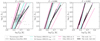 |
Fig. 1. HRDs for metallicities Z = 0.014 (Solar, left), Z = 0.006 (LMC, middle), and Z = 0.002 (SMC, right). Solid black lines show predicted IS boundaries from A16 for the second+third crossings averaged together; dashed black lines show the first crossing. Solid and dashed cyan lines illustrate predicted boundaries from De Somma et al. (2020, 2022, with their case A referred to as a ‘canonical’ mixing-length relation. We note the difference in Z values: 0.020, 0.008, 0.004), for αML = 1.7 and 1.5, respectively. Solid and dashed pink lines show predicted sets A (simple convective model) and D (added radiative cooling, turbulent pressure and flux) from Deka et al. (2024), which estimate the envelopes of instability strips across a large range of metallicities ([M/H] ∈ {0.00, −0.34, −0.75}, namely, Z∈ {0.013, 0.006, 0.002}) and are shown in all panels. Observational estimates of 265 fundamental-mode Galactic classical Cepheids from Groenewegen (2020a) are shown in the left panel. Empirically derived IS boundaries for the LMC from Espinoza-Arancibia et al. (2024) are shown as grey regions in the middle panel. |
On the theory side, De Somma et al. (2020, 2022) computed IS boundaries based on non-linear hydrodynamical models assuming three different mass-luminosity relations during the Cepheid stage: case A was computed for ‘canonical’ models (i.e. without convective core overshooting, rotation, and mass loss); cases B & C considered ad hoc increases in luminosity at fixed mass by adding Δlog L = 0.2 and 0.4 dex to the canonical model, respectively. De Somma et al. (2020, 2022) further considered sensitivity to the mixing-length parameter αML. Figure 1 displays their IS edges for canonical models with αML = 1.7, as well as αML = 1.5 in the Solar case (Z = 0.02 in their models). The comparison with observations shows that the position of the blue IS boundary in these models is generally too cold, over the entire luminosity range at Solar metallicity and at low luminosities in the case of the MCs. However, the red edges at LMC and SMC metallicity agree well with our predictions. Last, but not least, we overlay IS boundaries computed using MESA from Deka et al. (2024) who tested several assumptions related to convection. Figure 1 gives their set A, which is a simple convection model, as well as their set D, where all radiative cooling, turbulent pressure, and turbulent flux are included simultaneously. Unfortunately, the Teff-L relations provided in Deka et al. (2024) represent envelopes dedicated to models spanning the metallicity range Z ∈ {0.013, 0.006, 0.002} (or [M/H] ∈{0.00, −0.34, −0.75}); thus, they cannot be assessed for metallicity effects. In particular, set D is much wider than allowed by the empirical constraints in the MW and the LMC. The narrower set A matches the locations of our predicted IS at SMC metallicity and otherwise predicts a bluer boundary than supported by observations.
In our approach, all models in the three-dimensional grid (ℳ, Z, ω) were initialised at the ZAMS and the evolutionary tracks were calculated until the end of core Helium burning. This helped ensure consistency among the computed models because physical effects that modify the mass-luminosity relation, such as overshooting, rotation, and mass loss, were considered throughout the evolution of the star. Conversely, ad hoc increases in the luminosity of Cepheid models, as implemented in cases B & C in De Somma et al. (2020, 2022), cannot be attributed to specific physical origins; thus, they do not self-consistently track the influence of convective core overshooting, for example, on the evolution of the star.
2.3. Computing synthetic Cepheid populations with SYCLIST
We computed synthetic populations using the Geneva population synthesis code SYCLIST (Georgy et al. 2014), which we adapted to output data required to distinguish the properties of primary and secondary stars in binary systems. The simulated populations mimic a constant star formation rate by adding together 296 synthetic star clusters with a mass of 50 ⋅ 103 M⊙ in the age range [5, 300] Myr (i.e. using a time step of 1 Myr) for each of the three metallicity values: Z = 0.014, 0.006, and 0.002. We used SYCLIST default parameters, such as a Salpeter (1955) initial mass function between 1.7 and 15 M⊙, the angular velocity distribution from Huang et al. (2010), a random spatial distribution of the rotation axis of the star sin(i) for the angle of view, a gravity darkening law following Espinosa Lara & Rieutord (2011), limb darkening based on Claret (2000), and a 30% probability of a star being in a binary system where the companion mass cannot be lower than 1.7 M⊙ (much lower masses are not photometrically relevant for what we are doing) due to the limitations of the grid. This should be considered when comparing to multiplicity fractions reported by observational studies, which may be significantly higher (e.g. Kervella et al. 2019; Evans et al. 2020; Shetye et al. 2024). In addition, since we use the same binary fraction for all metallicity values, its exact value does not matter for the determination of the metallicity effect.
SYCLIST relies on single-star evolution tracks computed with the Geneva stellar evolution code. Hence, the treatment of binary stars is simplistic, and neither binary evolution (Neilson et al. 2015; Karczmarek et al. 2023; Dinnbier et al. 2024) nor cluster dynamics (Dinnbier et al. 2022) are taken into account. Multiplicity is tagged by the Bin flag, which can take four different values. Single stars are flagged as Bin= = 0. Stars flagged with Bin= = 2 are cases where the mass of the secondary is lower than the minimum mass allowed by the grid of models (and we decided to remove them from our sample). Finally, Bin= = 1 and Bin= = 3 correspond to the primary and secondary components of a binary system.
We considered a Cepheid as any (individual) non-MS (log g < 3.4) star whose luminosity, L. and effective temperature, Teff, fall within the IS boundaries determined using the same models (A16). For binary systems, we considered the L and Teff values for individual components to determine whether a star is a Cepheid. The blue edge was averaged over the second and third crossings, while for the red edge, we used both boundaries corresponding to the first crossing and second+third crossings; here, the transition occurs where they intersect with one another: at (log Teff, log L) values of (3.72, 3.19), (3.74, 3.14), and (3.76, 2.76) for the MW, LMC, and SMC, respectively. When necessary, IS edges can be extended to lower or higher luminosities to include stars falling outside of their range. The position of blue loops is imprinted on the location of stars in these HRDs, as can be seen from the red dashed lines in Fig. 2. We limited the number of first crossing Cepheids by only considering stars more luminous than these lines, defined by the following two (log Teff, log L) points {(3.7962, 3.027), (3.7510, 2.7662)}, {(3.8035, 3.027), (3.7564, 2.7698)}, and {(3.8194, 2.610), (3.7761, 2.4952)} for Z = 0.014, 0.006, and 0.002, respectively. These cuts are defined where there is an apparent drop in the density of stars as we move towards a lower luminosity level along the IS, which we associate with the extremely rapid Hertzsprung gap phase. We note that this distinction becomes more difficult as we move to lower metallicities; for instance, at Z = 0.002. This is because the minimum mass of Cepheids on the second+third crossings decreases with decreasing metallicity (A16). Hence, some contamination might remain in our selection, but it is expected to be fairly negligible. We compiled a total of 8332, 15043, and 24289 Cepheids selected for Z = 0.014, 0.006, and 0.002, respectively. The resulting Cepheid populations, whose HRDs are illustrated on Fig. 2, are well sampled and thus suitable for determining the effect of metallicity on LLs. They can also be used to make comparisons with key features of observed populations. To this end, we generally compare MW Cepheids to predictions at Solar metallicity (Z = 0.014), LMC Cepheids to Z = 0.006, and SMC Cepheids to Z = 0.002. However, we caution that observed Cepheid populations are generally more complex than our synthetic populations; notably, with respect to star formation history, non-unique values of metallicity, and stellar multiplicity. Additionally, we caution that many MW Cepheids with high-quality spectroscopic observations have super-Solar abundances, exceeding the range of the models.
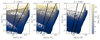 |
Fig. 2. HRDs for all 296 SYCLIST cluster simulations at each metallicity considered: Z = 0.014 (left), Z = 0.006 (middle), and Z = 0.002 (right). The colour scale indicates the initial mass of the star, from the least (blue) to the most massive ones (yellow). Overlaid in black are the IS boundaries determined by A16 for the second+third crossings averaged together (solid) and first crossing (dashed). Red dashed lines show the cut applied to exclude most of the first-crossing stars. |
The luminosities were translated to magnitudes in several photometric passbands to facilitate comparisons with observations. We used empirical calibrations by Worthey & Lee (2011) to compute the colours and magnitudes. The latter take log g, [M/H], and Teff as input parameters, with Mbol, ⊙ = 4.75 mag, and return several colour indices (i.e. U − B, B − V, V − R, V − I, J − K, H − K, and V − K) as well as the bolometric correction for the V-band magnitude. Using predicted combinations of V-band magnitudes and colours, we obtained magnitudes for the I, J, H, and Ks filters. Colour transformations based on V − I1 allowed us to derive Gaia magnitudes G, GBP, and GRP. We also made use of the transformations between ground-based and Hubble Space Telescope (HST) system apparent magnitudes empirically determined by Breuval et al. (2020, Sect. 2.3), in the F160W, F555W, and F814W passbands. Furthermore, we used the JWST magnitude conversion tool2 to compute magnitudes in the NIRCam F090W, F115W, F150W, F277W, F356W, and F444W bands, using predicted V and Ks-band magnitudes. Using combinations of various passbands, we computed the following reddening-free Wesenheit magnitudes (Madore 1982) assuming a Fitzpatrick (1999) reddening law with RV = 3.1 ± 0.1, following B22, as per their Table 3:
 (4)
(4)
 (5)
(5)
 (6)
(6)
 (7)
(7)
 (8)
(8)
In the case of non-spherical stars, SYCLIST applies corrections to predicted values of L and Teff to account for the effects of: the angle of view, the angular velocity, gravity darkening, and limb darkening. The effects on these stellar properties are at the level of ∼0.1% for the luminosity and ∼0.01% for the effective temperature for Cepheids. These corrections are discussed in more detail in Sects. 2.3.1 to 2.3.3 of Georgy et al. (2014). We discarded simulated Cepheids in binary systems where the constant flux of a companion star would significantly bias the Cepheid’s amplitude by more than 0.2 mag. Strongly contaminated Cepheids would typically not be discovered due to insufficient variability or cut from observed samples via σ clipping (cf. Anderson & Riess 2018).
We computed fundamental-mode pulsation periods, P, following the tight period-radius relations consistently derived by A16 (see their Table 5) using identical models. Averaging over different rotation rates, the blue and red edges of the IS, and the second+third crossings, we obtained metallicity-dependent fiducial period-radius relations at the centre of the IS:
 (9)
(9)
 (10)
(10)
 (11)
(11)
with 1σ dispersions of 0.025, 0.032, and 0.033, respectively. We accounted for the intrinsic width of the period-radius relation by adding a random offset to each period computed using Eqs. (9)–(11). The added offsets were normally distributed with zero mean and a standard deviation corresponding to one quarter of the mean period difference between the red and blue edges in the log R interval [1.8, 2.1] for the same metallicity value: 0.0148, 0.0217, and 0.0195 for Z = 0.014, 0.006, and 0.002, respectively. This is equivalent to assuming that the blue and red IS edges encompass > 99% of all possible periods.
3. Properties of the synthetic Cepheid populations
3.1. Predicted versus observed period distributions
Figure 3 compares our Cepheid populations to the observed fundamental-mode Cepheid period distributions of the MW (Pietrukowicz et al. 2021), LMC (Soszyński et al. 2015), and SMC (Soszyński et al. 2017). We generally found good agreement between observed and predicted period distributions considering the caveats involved in the comparison, notably concerning metallicity differences, with the peak of the distribution moving to shorter periods as the metallicity decreases. The modes of the predicted distributions agree well for the MW and the LMC. This is particularly important because the peak is dominated by the minimum mass at which models exhibit blue loops that enter the IS. The predicted distribution for Z = 0.002 suggests a slowly increasing number of Cepheids at periods longer than the mode of the observed distribution. This artefact of the age limit (< 300 Myr) applied here (e.g. a 2.5 d Z = 0.002 Cepheid at the IS centre, crossing averaged, is roughly 350 Myr old, cf. A16, their Table 4) has no bearing on the distance scale.
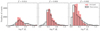 |
Fig. 3. Distribution of log P for Z = 0.014 (left), 0.006 (middle), and 0.002 (right panel). The SYCLIST populations appear in red, while observations are shown as black histograms. Observations come from Pietrukowicz et al. (2021) and Soszyński et al. (2015, 2017) for Classical Cepheids in the Milky Way and Magellanic Clouds, respectively. Observational counts have been rescaled in order to match the numbers we have in SYCLIST simulations, by a factor 3.4, 5.9, and 7.5 for Z = 0.014, 0.006, and 0.002, respectively. The age limit applied (< 300 Myr) to the synthetic populations leads to mismatches at the shortest periods, particularly at Z = 0.002. |
At periods longer than the peak, both simulated and observed distributions decline exponentially, and there is good agreement for the two lower-metallicity cases. The broader distribution of MW periods likely reflects the larger metallicity range of its constituent Cepheids and the more complex star formation history. As a side note, Anderson et al. (2017) previously showed a more significant mismatch in period distributions for first-overtone Cepheids compared to fundamental-mode Cepheids, although the origin of this mismatch remains unknown.
3.2. How Cepheids sample the instability strip
Evolutionary timescales vary along the blue loop. This could lead to a non-uniform sampling of the instability strip. Here, we compare the distributions of Cepheids in our synthetic population across the IS to a uniform distribution based on the positions of the IS edges.
We define a mid-IS line that bisects the blue and red edges, with a break at the intersection between the first crossing and the second+third crossings. Following this, we considered two different distributions:
-
A uniform distribution between the blue and red edges of the IS. For this, we uniformly generated 10 000 log L values between the minimum and maximum; namely, [1.1969, 4.9071], [1.362, 4.9969], and [1.4983, 5.0657] for Z = 0.014, 0.006, and 0.002, respectively. We then compute the corresponding log Teff on the blue and red sides, either based on the first or second+third crossings, depending on the luminosity, and again generate temperatures uniformly distributed between those edges;
-
The distribution obtained from SYCLIST.
We computed the difference between the log Teff of the above two distributions and that of the mid-IS line, which shows a break where the red boundary of the IS changes slope, so the resulting distributions are centred on zero. Then, a positive value would mean that the star is located more towards the blue edge of the IS (hotter Teff), while a negative value suggests that it falls on the redder side of the IS (cooler Teff). This is illustrated in Fig. 4. We would expect to see a roughly flat distribution if the IS was uniformly populated. There does not seem to be a significant predominance of bluer or redder stars for Z = 0.002. However, for Z = 0.006 (and to a lesser extent Z = 0.014) stars seem to pile up towards the red IS edge. Hence, our SYCLIST populations demonstrate that Cepheids are not uniformly distributed in Teff within the IS.
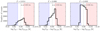 |
Fig. 4. Distribution of log Teff − log Teff, mid for our selection of IS stars in SYCLIST simulations, where log Teff, mid corresponds to the effective temperature at the mid-IS line right in the middle between the blue and red edges of the IS, for Z = 0.014 (left), 0.006 (middle), and 0.002 (right panel). The vertical lines indicate the 1σ dispersion that would correspond to a uniform distribution of stars within the IS. |
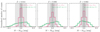 |
Fig. 7. LL scatter in the V-band (green) and WH magnitudes (pink), for Z = 0.014 (left), 0.006 (middle), and 0.002 (right panel). The histograms show the difference in magnitude between the individual SYCLIST IS stars and that of the SYCLIST LL fit at the same log P. The shaded regions correspond to the standard deviation, hence to the scatter of the LL and the values are reported on the plot with the corresponding colour. |
3.3. The intrinsic scatter of the Leavitt law
We proceed with the translation of modelled quantities (i.e. the intrinsic luminosity and radius of the star) to observables that can then allow us to make comparisons with observational studies. We fit linear LLs for each combination of photometric band and metallicity to the SYCLIST populations of IS stars. After which, we fit the resulting intercept and slope parameters to obtain αM and βM. To this end, we use the formalism from Sect. 1 (Eqs. 1–3). We also cross-checked these results against the mid-points of the individual IS edges, where LL are first fitted separately on the blue and red edges and blue-red averaged intercept and slope are then used to derive metallicity parameters.
Width of the instability strip, as measured in the observations and predicted with our models.
Figures 5 and 6 show the LL fits obtained for the V-band and WH magnitudes. We highlight the fits based on the SYCLIST population of IS stars, but we also show those corresponding to the blue and red edges separately, as well as the average between the two with the break where the red slope switches from the first crossing to the second+third crossings. Slight differences appear between the SYCLIST and mid-IS fit and their impact on the resulting metallicity parameters αM and βM are discussed in the following section. These differences are to be expected because the IS is not uniformly populated across temperature, as shown in Sect. 3.2.
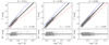 |
Fig. 5. Top: LLs in the V band, for Z = 0.014 (left), 0.006 (middle), and 0.002 (right panel). IS stars from SYCLIST are shown as grey points. The blue and red lines correspond to the IS boundaries from A16. The black solid line is the LL fit to the SYCLIST population, for log P0 = 0.0. The corresponding slope value, β, is annotated on the bottom right of each panel. The black dashed line shows the mid-IS fit, obtained by averaging the magnitude values for the blue and red boundaries at a given period. It shows a break in slope where the transition between the red edges for first crossing and second+third crossings occurs. Note: the varying axis ranges. Bottom: Residuals computed as the difference in magnitude between the individual SYCLIST stars and that of the SYCLIST LL fit at the same period. |
For the SH0ES Wesenheit magnitude, WH, we found a slope of −3.243 at LMC metallicity and we note that this is in very close agreement with the global LL slope adopted in R22, −3.299 ± 0.015 mag dex−1, which is strongly constrained by 339 LMC Cepheids with precise photometry from the ground and from HST. Figures of LL fits for other magnitudes are provided via Zenodo3, and the fits parameters are provided for the SYCLIST populations either using a free or fixed slope, the blue and red IS edges separately, and the midline between the two IS edges in Appendix B: Tables B.1, B.2, B.3, B.4, and B.5, respectively. We also note that an increase in the binary fraction (see Sect. 2.3) could have a noticeable effect on the absolute values of the LL intercept. However, we only report these values for completeness and do not draw any direct conclusions from them, as the main focus of this study is the assessment of the metallicity dependence in a differential sense.
We consider the LL scatter as an important diagnostic for the quality of our synthetic populations. It is an empirical fact that arises from the width of the IS. Observations exhibit a decrease in scatter as one moves towards redder filters and also for Wesenheit magnitudes (e.g. Madore & Freedman 2012). This wavelength dependence can be attributed to the connection between the intrinsic LL scatter and the period-luminosity-colour relation. As expected, the LL scatter for the WH magnitude is lower with respect to the one for the V band. The overall dispersion gets slightly smaller as the metallicity decreases when using the V band, but we have the opposite effect for WH. Figure 7 shows the distribution of the residuals, as an illustration of the LL scatter, for the V and WH magnitudes. We found 0.207 and 0.075 mag for the V and WH magnitudes at LMC metallicity, while observations have reported values of 0.22 and 0.069 mag. The latter value was used as a finite width for the WH LL, and obtained by subtracting quadratically the photometric measurement errors (0.03 mag) to the observed dispersion (0.075 mag, R22). We provide in Table 1 the predicted scatter values we obtain for all the magnitudes, at each metallicity value. We also quote the observationally derived scatters for comparison. We find that there is a generally very good agreement between these two. Our predicted scatters fall typically within ±0.01 − 0.02 mag of the observed values, when comparing with Z = 0.006, given that most studies focused on the LMC. Furthermore, we find the same trend, where the scatters are larger for bluer wavelengths, and get smaller as we go towards redder filters. Also, even if we were to consider single stars only in our simulations, by not accounting for the flux contribution of companion stars, the impact on our predicted scatters would be negligible.
4. Metallicity dependence of the Cepheid LL
The previous sections established that the models considered here provide a very close match to a) the position of the IS; b) the period distribution of Cepheids at the respective metallicities; and c) the width of the IS across many wavelengths. Additionally, the slope of the predicted WH LL for LMC metallicity is a close match to the global slope adopted in SH0ES (R22). Furthermore, A16 demonstrated very good agreement among predicted and observed: a) period changes (recently also shown using period changes measured from radial velocities; Anderson et al. 2024), b) masses; c) radii; and d) flux-weighted gravity (Anderson et al. 2020; Groenewegen 2020b). The following compares the predicted dependence of the LL on metallicity to observational results reported in the recent literature. Figures 5 and 6 illustrate LLs derived from our synthetic populations; additional figures are available via Zenodo.
Metallicity parameters βM and αM predicted with SYCLIST populations, either letting the LL slope vary or be fixed to the LMC value (last two columns), for different pivot periods: log P0 = 0.0, 0.7, and 1.0.
4.1. The LL slope-metallicity dependence
The predicted slope-metallicity dependence (βM ≠ 0) was first reported by A16 and confirmed by other stellar models (De Somma et al. 2022). Here, we find that our synthetic LLs also exhibit a slope-metallicity dependence in all individual filters and Wesenheit magnitudes, in the sense that LL slopes become steeper (more negative) at lower metallicity; namely, βM > 0 in Eq. (3). We fit the slope component of Eq. (3) to derive βM for individual filters and Wesenheit magnitudes, as reported in Table 2. The left panel of Fig. 8 illustrates our SYCLIST predictions as a function of wavelength. They range from ∼0.13, at redder wavelengths, to ∼0.38, at bluer wavelengths.
The predicted slope-metallicity dependence is supported by observations. Table 2 in Soszyński et al. (2015, OGLE-III Magellanic Cloud Cepheids) reveals that the LL slope is steeper among the lower metallicity SMC Cepheids in all of I-, V-, and Wesenheit, WVI, magnitudes for Cepheids pulsating in the fundamental mode and the first and second overtones. Although the difference reaches > 10σ significance in the optimal case of fundamental-mode Cepheids in WVI, no note on this issue was made. Table 4 in Breuval et al. (2021) lists LL slopes across a wider range of passbands for fundamental-mode Cepheids. While the reported uncertainties precluded establishing statistically significant trends, we noticed that all Wesenheit LLs yielded steeper slopes in the SMC compared to the LMC. Metallicity-dependent slopes have also been investigated using MW Cepheids with direct spectroscopic abundance measurements, although no significant effect has been established for now (e.g. Ripepi et al. 2020; Trentin et al. 2024).
Nonetheless, it is worth pointing out that Figs. 4 and A1 in Trentin et al. (2024) suggest a preference for a slope dependence (their parameter δ) of the order of βFe ≈ 0.1 mag dex−1 (log P/P0)−1 for fundamental -mode and first-overtone Cepheids and βFe ≈ 0.2 mag dex−1 (log P/P0)−1 for fundamental-mode Cepheids alone. Their βFe are also displayed on Fig. 8. Although their approach differs from ours, in that they only used MW Cepheids with a broad range of [Fe/H], their results still show a very good agreement with our model predictions. We note that Trentin et al. (2024) reported a ∼0.1 mag dex−1 lower value for αFe when neglecting the slope-metallicity dependence.
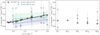 |
Fig. 8. Metallicity effect on the LL slope, βM, as defined in Eq. (3). The left panel shows βM as a function of the effective wavelength 1/λ, while the right panel shows the comparison for Wesenheit magnitudes. Our predictions based on SYCLIST are shown in black. Observational results from Trentin et al. (2024) are shown for the fundamental-mode and first-overtone Cepheids and fundamental-mode Cepheids alone in blue and green, respectively. In the left panel, the vertical dotted lines show the location of all the photometric passbands considered, and we label some of them to orient the reader. |
4.2. The LL intercept-metallicity dependence
As mentioned in Sect. 4.1, αM depends on pivot period if βM ≠ 0. Values of αM must therefore be accompanied by the corresponding P0. Additionally, care must be taken to compare predictions to observational studies based on equivalent approaches, since the majority of observational studies assume a universal LL slope (i.e. βM = 0). To facilitate comparisons with observational studies, we report our results in Table 2 for log P0 = 0.0, 0.7, and 1.0 for a wide range of passbands from optical to infrared wavelengths.
Figure 9 illustrates the metallicity dependence of the LL intercept, α, for log P0 = 1.0, with β as a free parameter. Then, α exhibits a mild dependence on metallicity, which increases with wavelength and is nearly flat around the I-band. The predicted trends with [M/H] appear to be non-linear, in particular at the shortest and longest wavelengths, and flatten off towards lower [M/H], resembling the trend reported based on observations in Breuval et al. (2024, their Fig. 8). Nevertheless, we determined αM using a linear fit to the three points, in keeping with the literature. Predictions at super-Solar [M/H] would help to constrain a possible non-linear trend.
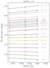 |
Fig. 9. LL intercepts α determined from synthetic Cepheid populations as a function of metallicity [M/H] for the different single-wavelength and Wesenheit magnitudes considered and for log P0 = 1.0. Some lines are shifted vertically, as indicated by the labels, to improve the readability of the plot. See Table 2 for the αM values associated to these fits. |
4.2.1. Wavelength dependence
Figure 10 illustrates the wavelength dependence of the LL intercept-metallicity effect αM determined from the linear fits in Fig. 9. The left panel shows our predictions for log P0 = 0.7 to allow for a direct comparison with the observational study by B22. Predictions based on SYCLIST populations are shown in black when β is a free parameter and in pink when β is fixed by our Z = 0.006 (LMC) results. Predictions based on the IS midline are shown in grey. The SYCLIST populations yield a slightly steeper wavelength dependence of αM, although the difference is hardly significant, reaching a maximum of 0.03 mag dex−1 at the shortest wavelengths. Fixing the slope does not affect the predicted wavelength dependence significantly. Table 2 tabulates the predictions based on the SYCLIST populations shown in Fig. 10, Table C.1 the values for predictions based on the IS bisector.
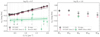 |
Fig. 10. Metallicity effect on the LL intercept, αM, as defined in Eq. (3). The left panel shows αM as a function of the effective wavelength 1/λ for a pivot period of log P0 = 0.7, while the right panel shows the comparison for Wesenheit magnitudes and for log P0 = 1.0. Our predictions based on SYCLIST, letting the LL slope vary or be fixed to that of the LMC, and IS edges are shown in black, pink, and grey, respectively. Observational results from B22 and SH0ES (R22) are shown in green in the left and right panels, respectively. In the left panel, the vertical dotted lines show the location of all the photometric passbands considered and we label some of them to orient the reader. |
The observational study by B22 relied on the metallicity differences between MW, LMC, and SMC Cepheids to investigate αFe effects using an LL slope fixed by the Cepheids in the LMC and log P0 = 0.7. We considered this study to be the most similar in approach to our predictions, since each of the three Cepheid groups featured a small range in metallicity. The determination of absolute magnitudes was particularly robust with respect to distance precision and (comparatively) low reddening. Further discussion of the varying level of (dis-)agreement among empirical studies has been provided by B22, Breuval et al. (2024), Bhardwaj et al. (2024), and Trentin et al. (2024), for example. Comparing measurements from B22 to our SYCLIST predictions with fixed LL slope (pink) reveals some disagreements at the level of 0.1 − 0.2 mag dex−1, with our values varying with 1/λ from −0.19 to −0.02 mag dex−1, while the values in B22 are more negative and exhibit a weaker dependence on 1/λ. At 1 μm, the difference is approximately 0.15 mag dex−1. We note that values attributed to A16 as reported in B22 were determined for log P0 = 0.0, rendering them more negative. Furthermore, we note that the discussion in Sect. 5.4 of B22 indicates that a more negative SMC metallicity ([Fe/H] = − 0.90 instead of −0.75) would tend to increase αFe by ∼0.05 mag dex−1, resulting in a better agreement with our predictions. However, the SMC’s updated iron abundance of −0.785 ± 0.012 (σ = 0.082) reported in Breuval et al. (2024) with attribution to Romaniello et al. (in prep.) does not support this. Instead, the order of magnitude and wavelength dependence of the difference with B22 could suggest a link to reddening. For example, the 0.2 mag dex−1 difference in V-band corresponds to a 0.15 mag difference assuming a 0.75 dex metallicity lever. Given the significant reddening of MW Cepheids (mean E(B − V) = 0.5 in Breuval et al. 2022), this difference could be explained by even a modest uncertainty in either E(B − V) or RV. Further works are required to investigate a possible reddening-related systematic in more detail. A detailed comparison with αFe values in Cruz Reyes & Anderson (2023, their Table 9) was foregone due to the limited metallicity range considered there (MW cluster Cepheids and LMC only), although their observational results generally agree with our predictions.
Figure 11 illustrates the behavior of the wavelength dependence of αM on pivot period ranging from 0.0 ≤ log P0 ≤ 1.5. Low values of log P0 = 0.0 yield a nearly constant αM with wavelength. However, the wavelength-dependence becomes increasingly stronger at higher log P0, exhibiting a positive trend, as shown in Fig. 10. Lastly, we note that the shortest wavelengths yield positive values for αM for log P0 ≳ 0.8. Positive intercept-metallicity effects at λ = 1 μm occur for log P0 ≳ 1.3, and αM < 0 for 1/λ ≲ 0.7, irrespective of log P0.
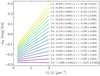 |
Fig. 11. Intercept-metallicity parameter αM as a function of the effective wavelength 1/λ for pivot periods ranging between log P0 = 0.0 (purple) and 1.5 (yellow), with a step of 0.1. The corresponding fits, based on SYCLIST populations, are annotated next to each line. |
4.2.2. Implications for the Hubble constant
As mentioned in Sect. 1, the impact of Cepheid metallicity on the measurement of H0 is largely mitigated by the rather small range of oxygen abundances among Cepheids in the high-mass spiral galaxies hosting type-Ia supernovae that is fully contained within the range of abundances of Cepheids in the host galaxies; notably, the MW, the LMC, and NGC 4258. Therefore, correcting differences in Cepheid luminosity due to chemical composition can improve the accuracy, rather than shifting the centre value (cf. Sect. 6.6 in R22). However, the intercept-metallicity effect of αM = −0.217 ± 0.046 measured as a free parameter of the SH0ES distance ladder (Riess et al. 2022, see their parameter γ) arguably provides the strongest empirical constraint for our theoretical predictions. This measurement is based on thousands of Cepheids across three anchor and 37 SN-host galaxies, relying exclusively on exquisite and homogeneous HST photometry, which is both insensitive to reddening thanks to infrared photometry and reddening-free by construction thanks to the use of Wesenheit magnitudes (for details, see Appendix D in R22). It further assumes a universal LL slope β = −3.299 ± 0.015, which is heavily informed by LMC Cepheids, and log P0 = 1.0.
Results based on SYCLIST populations adopting a fixed LL slope (β) derived at Z = 0.006 and using log P0 = 1.0 provide the closest correspondence to the observational setup of the SH0ES distance ladder. The right panel of Fig. 10 illustrates these results for several Wesenheit magnitudes. Adopting H-band Wesenheit magnitudes as used in the SH0ES distance ladder (Eq. 6) yields αM = −0.204 ± 0.030 mag dex−1, in excellent agreement with R22. Fixing β to the Z = 0.006 simulations reduces the predicted values for αM by 0.05 − 0.11 mag dex−1, depending on the Wesenheit magnitude considered. Tables 2 and C.1 report the predicted values for αM.
5. Summary and conclusions
In this work, we investigate the effect of chemical composition on the LL using synthetic populations of Cepheids computed using Geneva stellar evolution models, a pulsational instability analysis thereof, and the SYCLIST tool. We note that the Geneva models were calibrated to reproduce properties of massive main sequence stars and the Sun – and not of evolved stars such as Cepheids. All models in the initial grids (Ekström et al. 2012; Georgy et al. 2013) have been self-consistently computed as stellar tracks from the zero-age MS to well beyond core He burning. The synthetic populations computed using SYCLIST interpolate in mass and rotation rate at the original (fixed) metallicity at which the models were computed, with Z = 0.014, 0.006, and 0.002 representing the abundances of the Sun and intermediate-age stars in the LMC and SMC, respectively. Photometric contributions by companion stars were included to maximise realism.
We tested all predictions using observational constraints from the recent literature. Specifically, we demonstrated that our predictions closely reproduce observed IS boundaries, period distributions, LL slopes, and the intrinsic dispersion of the LL as a function of wavelength and metallicity. Additionally, we note that A16 previously demonstrated excellent agreement between predictions made by these same models and additional Cepheid properties, including mass-luminosity relations, period-radius relations, rates of period change, and so on. This extensive comparison demonstrates the high predictive power of this model set (Ekström et al. 2012; Georgy et al. 2013) for Cepheids.
Our simulations predict LL slopes, β, to depend on metallicity. This intriguing property of the Cepheid LL was previously predicted by A16 and has since been corroborated by another set of models (De Somma et al. 2022). Section 4.1 shows that observational studies confirm both the direction and magnitude of this effect, despite the measurement being challenging. We note that distance measurements based on Cepheids generally assume universal LL slopes and that further study is needed to test this important prediction. We further caution that the slope-metallicity dependence introduces a dependence of the intercept-metallicity effect on the pivot period (P0), which must be explicitly considered in comparisons among studies.
We found an excellent agreement in the intercept-metallicity dependence (αM) determined in analogy with the SH0ES distance ladder (R22), which provides the most stringent and direct empirical constraint to date (cf. Sect. 4.2.2). We therefore conclude that a) the Cepheid metallicity effect cannot bias the H0 measurement by design of the SH0ES distance ladder and b) our stellar models fully support the approach taken by R22. Comparisons with other empirical studies from the literature yield the best agreement for studies targeting low-extinction MW Cepheids with accurate parallaxes alongside LMC and SMC Cepheids that assume the well known detached eclipsing binary distances (Pietrzyński et al. 2019; Graczyk et al. 2020). However, disagreements at the level of 0.1 − 0.2 mag dex−1 become more significant at shorter wavelengths (Sect. 4.2), suggesting a possible origin rooted in reddening-related systematics.
Further work is needed to understand the veracity and implications of the LL slope-metallicity dependence, as well as a possible non-linearity in the intercept-metallicity dependence. Super-Solar metallicity models will be particularly useful to this end, along with improved parallaxes and astrometric systematics published in the fourth Gaia data release, scheduled for 2026.
Acknowledgments
We wish to thank the reviewer whose comments helped clarify and improve the paper. RIA & SK are funded by the SNSF through a Swiss National Science Foundation Eccellenza Professorial Fellowship (award PCEFP2_194638).
References
- Anderson, R. I., & Riess, A. G. 2018, ApJ, 861, 36 [NASA ADS] [CrossRef] [Google Scholar]
- Anderson, R. I., Ekström, S., Georgy, C., et al. 2014, A&A, 564, A100 [NASA ADS] [CrossRef] [EDP Sciences] [Google Scholar]
- Anderson, R. I., Saio, H., Ekström, S., Georgy, C., & Meynet, G. 2016, A&A, 591, A8 [NASA ADS] [CrossRef] [EDP Sciences] [Google Scholar]
- Anderson, R. I., Ekström, S., Georgy, C., Meynet, G., & Saio, H. 2017, Eur. Phys. J. Web Conf., 152, 06002 [Google Scholar]
- Anderson, R. I., Saio, H., Ekström, S., Georgy, C., & Meynet, G. 2020, A&A, 638, C1 [NASA ADS] [CrossRef] [EDP Sciences] [Google Scholar]
- Anderson, R. I., Viviani, G., Shetye, S. S., et al. 2024, A&A, 686, A177 [NASA ADS] [CrossRef] [EDP Sciences] [Google Scholar]
- Andrievsky, S. M., Kovtyukh, V. V., Luck, R. E., et al. 2002, A&A, 381, 32 [NASA ADS] [CrossRef] [EDP Sciences] [Google Scholar]
- Asplund, M., Grevesse, N., & Sauval, A. J. 2005, in Cosmic Abundances as Records of Stellar Evolution and Nucleosynthesis, eds. I. Barnes, G. Thomas, & F. N. Bash, ASP Conf. Ser., 336, 25 [NASA ADS] [Google Scholar]
- Bhardwaj, A., Riess, A. G., Catanzaro, G., et al. 2023, ApJ, 955, L13 [NASA ADS] [CrossRef] [Google Scholar]
- Bhardwaj, A., Ripepi, V., Testa, V., et al. 2024, A&A, 683, A234 [NASA ADS] [CrossRef] [EDP Sciences] [Google Scholar]
- Bono, G., & Stellingwerf, R. F. 1994, ApJS, 93, 233 [Google Scholar]
- Bresolin, F. 2011, ApJ, 729, 56 [Google Scholar]
- Breuval, L., Kervella, P., Anderson, R. I., et al. 2020, A&A, 643, A115 [EDP Sciences] [Google Scholar]
- Breuval, L., Kervella, P., Wielgórski, P., et al. 2021, ApJ, 913, 38 [NASA ADS] [CrossRef] [Google Scholar]
- Breuval, L., Riess, A. G., Kervella, P., Anderson, R. I., & Romaniello, M. 2022, ApJ, 939, 89 [NASA ADS] [CrossRef] [Google Scholar]
- Breuval, L., Riess, A. G., Casertano, S., et al. 2024, ApJ, 973, 30 [Google Scholar]
- Breuval, L., Anand, G. S., Anderson, R. I., et al. 2025, arXiv e-prints [arXiv:2507.15936] [Google Scholar]
- Claret, A. 2000, A&A, 363, 1081 [NASA ADS] [Google Scholar]
- Cruz Reyes, M., & Anderson, R. I. 2023, A&A, 672, A85 [NASA ADS] [CrossRef] [EDP Sciences] [Google Scholar]
- Cyburt, R. H., Fields, B. D., & Olive, K. A. 2003, Phys. Lett. B, 567, 227 [NASA ADS] [CrossRef] [Google Scholar]
- De Somma, G., Marconi, M., Molinaro, R., et al. 2020, ApJS, 247, 30 [Google Scholar]
- De Somma, G., Marconi, M., Molinaro, R., et al. 2022, ApJS, 262, 25 [NASA ADS] [CrossRef] [Google Scholar]
- De Somma, G., Marconi, M., Cassisi, S., et al. 2024, MNRAS, 528, 6637 [Google Scholar]
- Deka, M., Bellinger, E. P., Kanbur, S. M., et al. 2024, MNRAS, 530, 5099 [Google Scholar]
- Dinnbier, F., Anderson, R. I., & Kroupa, P. 2022, A&A, 659, A169 [NASA ADS] [CrossRef] [EDP Sciences] [Google Scholar]
- Dinnbier, F., Anderson, R. I., & Kroupa, P. 2024, A&A, 690, A385 [NASA ADS] [CrossRef] [EDP Sciences] [Google Scholar]
- Ekström, S., Georgy, C., Eggenberger, P., et al. 2012, A&A, 537, A146 [Google Scholar]
- Espinosa Lara, F., & Rieutord, M. 2011, A&A, 533, A43 [NASA ADS] [CrossRef] [EDP Sciences] [Google Scholar]
- Espinoza-Arancibia, F., Pilecki, B., Pietrzyński, G., Smolec, R., & Kervella, P. 2024, A&A, 682, A185 [NASA ADS] [CrossRef] [EDP Sciences] [Google Scholar]
- Evans, N. R., Günther, H. M., Bond, H. E., et al. 2020, ApJ, 905, 81 [CrossRef] [Google Scholar]
- Fitzpatrick, E. L. 1999, PASP, 111, 63 [Google Scholar]
- Genovali, K., Lemasle, B., Bono, G., et al. 2014, A&A, 566, A37 [NASA ADS] [CrossRef] [EDP Sciences] [Google Scholar]
- Georgy, C., Ekström, S., Granada, A., et al. 2013, A&A, 553, A24 [NASA ADS] [CrossRef] [EDP Sciences] [Google Scholar]
- Georgy, C., Granada, A., Ekström, S., et al. 2014, A&A, 566, A21 [NASA ADS] [CrossRef] [EDP Sciences] [Google Scholar]
- Gieren, W., Storm, J., Konorski, P., et al. 2018, A&A, 620, A99 [NASA ADS] [CrossRef] [EDP Sciences] [Google Scholar]
- Graczyk, D., Pietrzyński, G., Thompson, I. B., et al. 2020, ApJ, 904, 13 [Google Scholar]
- Grigahcène, A., Dupret, M. A., Gabriel, M., Garrido, R., & Scuflaire, R. 2005, A&A, 434, 1055 [NASA ADS] [CrossRef] [EDP Sciences] [Google Scholar]
- Groenewegen, M. A. T. 2020a, A&A, 635, A33 [EDP Sciences] [Google Scholar]
- Groenewegen, M. A. T. 2020b, A&A, 640, A113 [NASA ADS] [CrossRef] [EDP Sciences] [Google Scholar]
- Hertzsprung, E. 1913, Astron. Nachr., 196, 201 [NASA ADS] [Google Scholar]
- Huang, W., Gies, D. R., & McSwain, M. V. 2010, ApJ, 722, 605 [Google Scholar]
- Javanmardi, B., Mérand, A., Kervella, P., et al. 2021, ApJ, 911, 12 [Google Scholar]
- Karczmarek, P., Hajdu, G., Pietrzyński, G., et al. 2023, ApJ, 950, 182 [NASA ADS] [CrossRef] [Google Scholar]
- Kervella, P., Gallenne, A., Remage Evans, N., et al. 2019, A&A, 623, A116 [NASA ADS] [CrossRef] [EDP Sciences] [Google Scholar]
- Lauterborn, D., Refsdal, S., & Weigert, A. 1971, A&A, 10, 97 [NASA ADS] [Google Scholar]
- Leavitt, H. S. 1907, Ann. Harv. College Obs., 60, 87 [Google Scholar]
- Leavitt, H. S., & Pickering, E. C. 1912, Harv. College Obs. Circ., 173, 1 [Google Scholar]
- Lemasle, B., François, P., Piersimoni, A., et al. 2008, A&A, 490, 613 [NASA ADS] [CrossRef] [EDP Sciences] [Google Scholar]
- Macri, L. M., Stanek, K. Z., Bersier, D., Greenhill, L. J., & Reid, M. J. 2006, ApJ, 652, 1133 [NASA ADS] [CrossRef] [Google Scholar]
- Madore, B. F. 1982, ApJ, 253, 575 [NASA ADS] [CrossRef] [Google Scholar]
- Madore, B. F., & Freedman, W. L. 2012, ApJ, 744, 132 [NASA ADS] [CrossRef] [Google Scholar]
- Maeder, A. 1997, A&A, 321, 134 [NASA ADS] [Google Scholar]
- Mérand, A., Kervella, P., Breitfelder, J., et al. 2015, A&A, 584, A80 [NASA ADS] [CrossRef] [EDP Sciences] [Google Scholar]
- Miller, C. L., Neilson, H. R., Evans, N. R., Engle, S. G., & Guinan, E. 2020, ApJ, 896, 128 [Google Scholar]
- Neilson, H. R., Schneider, F. R. N., Izzard, R. G., Evans, N. R., & Langer, N. 2015, A&A, 574, A2 [NASA ADS] [CrossRef] [EDP Sciences] [Google Scholar]
- Persson, S. E., Madore, B. F., Krzemiński, W., et al. 2004, AJ, 128, 2239 [NASA ADS] [CrossRef] [Google Scholar]
- Pietrukowicz, P., Soszyński, I., & Udalski, A. 2021, Acta Astron., 71, 205 [NASA ADS] [Google Scholar]
- Pietrzyński, G., Graczyk, D., Gallenne, A., et al. 2019, Nature, 567, 200 [Google Scholar]
- Riess, A. G., Casertano, S., Yuan, W., Macri, L. M., & Scolnic, D. 2019, ApJ, 876, 85 [Google Scholar]
- Riess, A. G., Yuan, W., Macri, L. M., et al. 2022, ApJ, 934, L7 [NASA ADS] [CrossRef] [Google Scholar]
- Ripepi, V., Molinaro, R., Musella, I., et al. 2019, A&A, 625, A14 [NASA ADS] [CrossRef] [EDP Sciences] [Google Scholar]
- Ripepi, V., Catanzaro, G., Molinaro, R., et al. 2020, A&A, 642, A230 [NASA ADS] [CrossRef] [EDP Sciences] [Google Scholar]
- Ripepi, V., Catanzaro, G., Clementini, G., et al. 2022, A&A, 659, A167 [NASA ADS] [CrossRef] [EDP Sciences] [Google Scholar]
- Romaniello, M., Riess, A., Mancino, S., et al. 2022, A&A, 658, A29 [NASA ADS] [CrossRef] [EDP Sciences] [Google Scholar]
- Saio, H., Winget, D. E., & Robinson, E. L. 1983, ApJ, 265, 982 [Google Scholar]
- Salpeter, E. E. 1955, ApJ, 121, 161 [Google Scholar]
- Shetye, S. S., Viviani, G., Anderson, R. I., et al. 2024, A&A, 690, A284 [NASA ADS] [CrossRef] [EDP Sciences] [Google Scholar]
- Soszyński, I., Udalski, A., Szymański, M. K., et al. 2015, Acta Astron., 65, 297 [NASA ADS] [Google Scholar]
- Soszyński, I., Udalski, A., Szymański, M. K., et al. 2017, Acta Astron., 67, 297 [NASA ADS] [Google Scholar]
- Trahin, B., Breuval, L., Kervella, P., et al. 2021, A&A, 656, A102 [NASA ADS] [CrossRef] [EDP Sciences] [Google Scholar]
- Trentin, E., Ripepi, V., Catanzaro, G., et al. 2023, MNRAS, 519, 2331 [Google Scholar]
- Trentin, E., Ripepi, V., Molinaro, R., et al. 2024, A&A, 681, A65 [NASA ADS] [CrossRef] [EDP Sciences] [Google Scholar]
- Unno, W. 1967, PASJ, 19, 140 [NASA ADS] [Google Scholar]
- Walmswell, J. J., Tout, C. A., & Eldridge, J. J. 2015, MNRAS, 447, 2951 [NASA ADS] [CrossRef] [Google Scholar]
- Worthey, G., & Lee, H.-C. 2011, ApJS, 193, 1 [CrossRef] [Google Scholar]
- Zahn, J. P. 1992, A&A, 265, 115 [NASA ADS] [Google Scholar]
- Ziółkowska, O., Smolec, R., Thoul, A., et al. 2024, ApJS, 274, 30 [CrossRef] [Google Scholar]
Appendix A: Terminology related to the metallicity dependence
Following the terminology used in the current paper, the general form of a LL is α + β ⋅ log(P/P0), with pivot period P0. Higher orders in log P as used, for instance, for Miras would then follow with γlog P2. In principle, α and β can both be metal dependent, and this can be written as α = α0 + αFe[Fe/H] to indicate an effect related to iron abundance, and analogously for β. The benefits of using this nomenclature is that a) subscript 0 always identifies the fiducial quantity for slope, intercept, and pivot period; b) subscripts can be used to distinguish between different effects/elements considered; c) it is immediately clear which metallicity dependence is discussed, which is more difficult if β = δ + γ[Fe/H], for instance. Table A.1 provides the equivalence between our terminology in Eq. (3) and those used in the recent literature.
Equivalence for the terminology in the LL parameters between our work and the recent literature.
Appendix B: Leavitt laws parameters for single-wavelength passbands and Wesenheit magnitudes
LL slope and intercepts for the SYCLIST populations of IS stars, for different pivot periods: log P0 = 0.0, 0.7, and 1.0.
LL intercepts for the SYCLIST populations of IS stars, using a slope (β) fixed to the value for the LMC, for different pivot periods: log P0 = 0.0, 0.7, and 1.0.
LL slope and intercepts for the blue edge of the IS, for different pivot periods: log P0 = 0.0, 0.7, and 1.0.
LL slope and intercepts for the red edge of the IS, for different pivot periods: log P0 = 0.0, 0.7, and 1.0. Parameters for the edges corresponding to the first crossing, and the second and third crossing averaged together are given separately.
LL intercepts for the midline between the blue and red edges of the IS, for different pivot periods: log P0 = 0.0, 0.7, and 1.0.
Appendix C: Intercept-metallicity dependence for IS edges
Metallicity parameter αM predicted at the midpoint between the IS edges, for different pivot periods: log P0 = 0.0, 0.7, and 1.0.
All Tables
Width of the instability strip, as measured in the observations and predicted with our models.
Metallicity parameters βM and αM predicted with SYCLIST populations, either letting the LL slope vary or be fixed to the LMC value (last two columns), for different pivot periods: log P0 = 0.0, 0.7, and 1.0.
Equivalence for the terminology in the LL parameters between our work and the recent literature.
LL slope and intercepts for the SYCLIST populations of IS stars, for different pivot periods: log P0 = 0.0, 0.7, and 1.0.
LL intercepts for the SYCLIST populations of IS stars, using a slope (β) fixed to the value for the LMC, for different pivot periods: log P0 = 0.0, 0.7, and 1.0.
LL slope and intercepts for the blue edge of the IS, for different pivot periods: log P0 = 0.0, 0.7, and 1.0.
LL slope and intercepts for the red edge of the IS, for different pivot periods: log P0 = 0.0, 0.7, and 1.0. Parameters for the edges corresponding to the first crossing, and the second and third crossing averaged together are given separately.
LL intercepts for the midline between the blue and red edges of the IS, for different pivot periods: log P0 = 0.0, 0.7, and 1.0.
Metallicity parameter αM predicted at the midpoint between the IS edges, for different pivot periods: log P0 = 0.0, 0.7, and 1.0.
All Figures
|
Fig. 1. HRDs for metallicities Z = 0.014 (Solar, left), Z = 0.006 (LMC, middle), and Z = 0.002 (SMC, right). Solid black lines show predicted IS boundaries from A16 for the second+third crossings averaged together; dashed black lines show the first crossing. Solid and dashed cyan lines illustrate predicted boundaries from De Somma et al. (2020, 2022, with their case A referred to as a ‘canonical’ mixing-length relation. We note the difference in Z values: 0.020, 0.008, 0.004), for αML = 1.7 and 1.5, respectively. Solid and dashed pink lines show predicted sets A (simple convective model) and D (added radiative cooling, turbulent pressure and flux) from Deka et al. (2024), which estimate the envelopes of instability strips across a large range of metallicities ([M/H] ∈ {0.00, −0.34, −0.75}, namely, Z∈ {0.013, 0.006, 0.002}) and are shown in all panels. Observational estimates of 265 fundamental-mode Galactic classical Cepheids from Groenewegen (2020a) are shown in the left panel. Empirically derived IS boundaries for the LMC from Espinoza-Arancibia et al. (2024) are shown as grey regions in the middle panel. |
| In the text | |
|
Fig. 2. HRDs for all 296 SYCLIST cluster simulations at each metallicity considered: Z = 0.014 (left), Z = 0.006 (middle), and Z = 0.002 (right). The colour scale indicates the initial mass of the star, from the least (blue) to the most massive ones (yellow). Overlaid in black are the IS boundaries determined by A16 for the second+third crossings averaged together (solid) and first crossing (dashed). Red dashed lines show the cut applied to exclude most of the first-crossing stars. |
| In the text | |
|
Fig. 3. Distribution of log P for Z = 0.014 (left), 0.006 (middle), and 0.002 (right panel). The SYCLIST populations appear in red, while observations are shown as black histograms. Observations come from Pietrukowicz et al. (2021) and Soszyński et al. (2015, 2017) for Classical Cepheids in the Milky Way and Magellanic Clouds, respectively. Observational counts have been rescaled in order to match the numbers we have in SYCLIST simulations, by a factor 3.4, 5.9, and 7.5 for Z = 0.014, 0.006, and 0.002, respectively. The age limit applied (< 300 Myr) to the synthetic populations leads to mismatches at the shortest periods, particularly at Z = 0.002. |
| In the text | |
|
Fig. 4. Distribution of log Teff − log Teff, mid for our selection of IS stars in SYCLIST simulations, where log Teff, mid corresponds to the effective temperature at the mid-IS line right in the middle between the blue and red edges of the IS, for Z = 0.014 (left), 0.006 (middle), and 0.002 (right panel). The vertical lines indicate the 1σ dispersion that would correspond to a uniform distribution of stars within the IS. |
| In the text | |
|
Fig. 7. LL scatter in the V-band (green) and WH magnitudes (pink), for Z = 0.014 (left), 0.006 (middle), and 0.002 (right panel). The histograms show the difference in magnitude between the individual SYCLIST IS stars and that of the SYCLIST LL fit at the same log P. The shaded regions correspond to the standard deviation, hence to the scatter of the LL and the values are reported on the plot with the corresponding colour. |
| In the text | |
|
Fig. 5. Top: LLs in the V band, for Z = 0.014 (left), 0.006 (middle), and 0.002 (right panel). IS stars from SYCLIST are shown as grey points. The blue and red lines correspond to the IS boundaries from A16. The black solid line is the LL fit to the SYCLIST population, for log P0 = 0.0. The corresponding slope value, β, is annotated on the bottom right of each panel. The black dashed line shows the mid-IS fit, obtained by averaging the magnitude values for the blue and red boundaries at a given period. It shows a break in slope where the transition between the red edges for first crossing and second+third crossings occurs. Note: the varying axis ranges. Bottom: Residuals computed as the difference in magnitude between the individual SYCLIST stars and that of the SYCLIST LL fit at the same period. |
| In the text | |
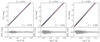 |
Fig. 6. Same as Fig. 5 for the WH magnitude. |
| In the text | |
|
Fig. 8. Metallicity effect on the LL slope, βM, as defined in Eq. (3). The left panel shows βM as a function of the effective wavelength 1/λ, while the right panel shows the comparison for Wesenheit magnitudes. Our predictions based on SYCLIST are shown in black. Observational results from Trentin et al. (2024) are shown for the fundamental-mode and first-overtone Cepheids and fundamental-mode Cepheids alone in blue and green, respectively. In the left panel, the vertical dotted lines show the location of all the photometric passbands considered, and we label some of them to orient the reader. |
| In the text | |
|
Fig. 9. LL intercepts α determined from synthetic Cepheid populations as a function of metallicity [M/H] for the different single-wavelength and Wesenheit magnitudes considered and for log P0 = 1.0. Some lines are shifted vertically, as indicated by the labels, to improve the readability of the plot. See Table 2 for the αM values associated to these fits. |
| In the text | |
|
Fig. 10. Metallicity effect on the LL intercept, αM, as defined in Eq. (3). The left panel shows αM as a function of the effective wavelength 1/λ for a pivot period of log P0 = 0.7, while the right panel shows the comparison for Wesenheit magnitudes and for log P0 = 1.0. Our predictions based on SYCLIST, letting the LL slope vary or be fixed to that of the LMC, and IS edges are shown in black, pink, and grey, respectively. Observational results from B22 and SH0ES (R22) are shown in green in the left and right panels, respectively. In the left panel, the vertical dotted lines show the location of all the photometric passbands considered and we label some of them to orient the reader. |
| In the text | |
|
Fig. 11. Intercept-metallicity parameter αM as a function of the effective wavelength 1/λ for pivot periods ranging between log P0 = 0.0 (purple) and 1.5 (yellow), with a step of 0.1. The corresponding fits, based on SYCLIST populations, are annotated next to each line. |
| In the text | |
Current usage metrics show cumulative count of Article Views (full-text article views including HTML views, PDF and ePub downloads, according to the available data) and Abstracts Views on Vision4Press platform.
Data correspond to usage on the plateform after 2015. The current usage metrics is available 48-96 hours after online publication and is updated daily on week days.
Initial download of the metrics may take a while.