| Issue |
A&A
Volume 702, October 2025
|
|
|---|---|---|
| Article Number | A206 | |
| Number of page(s) | 19 | |
| Section | Extragalactic astronomy | |
| DOI | https://doi.org/10.1051/0004-6361/202556140 | |
| Published online | 24 October 2025 | |
The ALPINE-CRISTAL-JWST survey: Spatially resolved star formation relations at z ∼ 5
1
Université de Strasbourg, CNRS, Observatoire Astronomique de Strasbourg, UMR 7550, 67000 Strasbourg, France
2
Université Côte d’Azur, Observatoire de la Côte d’Azur, CNRS, Laboratoire Lagrange, 06000 Nice, France
3
Aix Marseille Univ, CNRS, CNES, LAM, Marseille, France
4
INAF – Osservatorio di Astrofisica e Scienza dello Spazio di Bologna, Via Gobetti 93/3, 40129 Bologna, Italy
5
Instituto de Estudios Astrofísicos, Facultad de Ingeniería y Ciencias, Universidad Diego Portales, Av. Ejército 441, Santiago, Chile
6
Millenium Nucleus for Galaxies (MINGAL), Concepción, Chile
7
Departamento de Astronomía, Universidad de Concepción, Barrio, Universitario, Concepción, Chile
8
Dipartimento di Fisica e Astronomia, Universitè di Padova, Vicolo dell’Osservatorio 3, Padova, Italy
9
INAF – Osservatorio Astronomico di Padova, Vicolo dell’ Osservatorio 5, 35122 Padova, Italy
10
International Centre for Radio Astronomy Research (ICRAR), The University of Western Australia, M468, 35 Stirling Highway, Crawley, WA 6009, Australia
11
ARC Center of Excellence for All Sky Astrophysics in 3 Dimensions (ASTRO 3D), Canberra, Australia
12
Sterrenkundig Observatorium, Ghent University, Krijgslaan 281 - S9, B9000 Ghent, Belgium
13
Department of Astronomy, University of Geneva, Chemin Pegasi 51, 1290 Versoix, Switzerland
14
Institut d’Astrophysique de Paris, Sorbonne Université, CNRS, UMR 7095, 98 bis bd Arago, 75014 Paris, France
15
IPAC, California Institute of Technology, 1200 E California Boulevard, Pasadena, CA 91125, USA
16
Center for Frontier Science, Chiba University, 1-33 Yayoi-cho, Inage-ku, Chiba 263-8522, Japan
17
Dipartimento di Fisica e Astronomia, Università degli Studi di Firenze, Via G. Sansone 1, 50019 Sesto Fiorentino, Firenze, Italy
18
INAF – Osservatorio Astrofisico di Arcetri, Largo E. Fermi 5, 50125 Firenze, Italy
19
Hiroshima Astrophysical Science Center, Hiroshima University, 1-3-1 Kagamiyama, Higashi-Hiroshima, Hiroshima 739-8526, Japan
20
Space Telescope Science Institute, 3700 San Martin Drive, Baltimore, MD 21218, USA
21
Gemini Observatory, NSF NOIRLab, 670 N. A’ohoku Place, Hilo, Hawai’i 96720, USA
22
Department of Physics and Astronomy, University of California, Davis, One Shields Ave., Davis, CA 95616, USA
23
Department of Physics and Astronomy and George P. and Cynthia Woods Mitchell Institute for Fundamental Physics and Astronomy, Texas A&M University, 4242 TAMU, College Station, TX 77843-4242, USA
24
Department of Physics and Astronomy, University of California, Riverside, 900 University Avenue, Riverside, CA 92521, USA
25
Instituto de Física y Astronomía, Universidad de Valparaíso, Avda. Gran Bretaña 1111, Valparaíso, Chile
26
INAF – Osservatorio astronomico d’Abruzzo, Via Maggini SNC, 64100 Teramo, Italy
27
National Centre for Nuclear Research, ul. Pasteura 7, 02-093 Warsaw, Poland
28
Dipartimento di Fisica e Astronomia “Augusto Righi”, Alma Mater Studiorum, Università di Bologna, Via Gobetti 93/2, 40129 Bologna, Italy
29
Dept. Fisica Teorica y del Cosmos, Universidad de Granada, Granada, Spain
30
Max-Planck-Institut für Radioastronomie, Auf dem Hügel 69, 53121 Bonn, Germany
31
Scuola Internazionale Superiore Studi Avanzati (SISSA), Physics Area, Via Bonomea 265, 34136 Trieste, Italy
32
Departamento de Astronomía, Universidad de Concepción, Barrio Universitario, Concepción, Chile
33
Department of Astronomy and Yonsei University Observatory, Yonsei University, Seoul 03722, Republic of Korea
34
Institute of Astronomy, Graduate School of Science, The University of Tokyo, 2-21-1 Osawa, Mitaka, Tokyo 181-0015, Japan
⋆ Corresponding author: This email address is being protected from spambots. You need JavaScript enabled to view it.
Received:
27
June
2025
Accepted:
15
August
2025
Abstract
Context. Star formation governs galaxy evolution, shaping stellar mass assembly and gas consumption across cosmic time. The Kennicutt-Schmidt (KS) relation, linking the star formation rate (SFR) and gas surface densities, is fundamental to understand star formation regulation, yet remains poorly constrained at z > 2 due to observational limitations and uncertainties in locally calibrated gas tracers. The [CII] 158 μm line has recently emerged as a key probe of the cold ISM and star formation in the early Universe.
Aims. We investigate whether the resolved [CII]–SFR and KS relations established at low redshift remain valid at 4 < z < 6 by analysing 13 main-sequence galaxies from the ALPINE and CRISTAL surveys, using multi-wavelength data (HST, JWST, ALMA) at ∼2 kpc resolution.
Methods. We performed pixel-by-pixel spectral energy distribution (SED) modelling with CIGALE on resolution-homogenised images. We developed a statistical framework to fit the [CII]–SFR relation that accounts for pixel covariance and compare our results to classical fitting methods. We tested two [CII]-to-gas conversion prescriptions to assess their impact on inferred gas surface densities and depletion times.
Results. We find a resolved [CII]–SFR relation with a slope of 0.87 ± 0.15 and intrinsic scatter of 0.19 ± 0.03 dex, which is shallower and tighter than previous studies at z ∼ 5. The resolved KS relation is highly sensitive to the [CII]-to-gas conversion factor: using a fixed global α[CII] yields depletion times of 0.5–1 Gyr, while a surface brightness-dependent W[CII], accounting for local ISM conditions, places some galaxies with high gas density in the starburst regime (< 0.1 Gyr).
Conclusions. Future inputs from both simulations and observations are required to better understand how the [CII]-to-gas conversion factor depends on local ISM properties. We need to break this fundamental limit to properly study the KS relation at z ≳ 4.
Key words: galaxies: high-redshift / galaxies: ISM / galaxies: star formation / submillimeter: galaxies / submillimeter: ISM
© The Authors 2025
 Open Access article, published by EDP Sciences, under the terms of the Creative Commons Attribution License (https://creativecommons.org/licenses/by/4.0), which permits unrestricted use, distribution, and reproduction in any medium, provided the original work is properly cited.
This article is published in open access under the Subscribe to Open model. This email address is being protected from spambots. You need JavaScript enabled to view it. to support open access publication.
1. Introduction
The study of star formation in the early Universe (z > 2) is a cornerstone of modern astrophysics, crucial for understanding galaxy evolution, mass assembly, and cosmic star formation history (SFH; e.g. Madau & Dickinson 2014; Freundlich 2024). The Kennicutt-Schmidt (KS) relation, linking star formation rate (SFR) surface density (ΣSFR) to gas surface density (Σgas) through a power law, has been fundamental for understanding the conversion of the gas into stars across cosmic time (e.g. Kennicutt 1998; de los Reyes & Kennicutt 2019). Initially proposed by Schmidt (1959) in terms of volume densities within the Milky Way, this relation was later reformulated for extrag alactic studies using measurements of surface densities (Kennicutt 1998). While extensively studied locally (e.g. Bigiel et al. 2008; Kennicutt & Evans 2012; Leroy et al. 2013; Pessa et al. 2021; Jiménez-Donaire et al. 2023), its high-redshift behaviour (z ≳ 2) remains poorly constrained, with significant uncertainties in both the slope and intrinsic scatter of the relation. These uncertainties arise primarily from low spatial resolution, limited sensitivity (e.g. Freundlich et al. 2013), and sample representativeness issues (e.g. Vallini et al. 2024), hindering progress towards an understanding of early-Universe star formation. Thanks to existing observational facilities such as Hubble Space Telescope (HST) and Atacama large millimetre/submillimetre array (ALMA), and the recent advancements made possible with the James Webb Space Telescope (JWST), we can now perform multi-wavelength analysis to probe galaxies at unprecedented redshifts and resolutions (e.g. Nagy et al. 2023; Hashimoto et al. 2023; Wang et al. 2023; Zavala et al. 2024). Those observations have opened new avenues for investigating the physical processes governing star formation in the first few billion years after the Big Bang.
Traditional molecular gas tracers, such as CO, become increasingly difficult to detect at higher redshift (z > 2, e.g. Molina et al. 2019; Tacconi et al. 2020), creating a critical gap in our understanding of early-Universe star formation (e.g. Genzel et al. 2010; Scoville et al. 2016). This limitation has been partially overcome by the use of the [CII] 158 μm emission line, now regularly used as an alternative tracer of molecular gas (Zanella et al. 2018). That fine-structure line is typically one of the most luminous far-infrared line in star-forming galaxies and is redshifted into ALMA’s atmospheric windows at z ≳ 4. This provides unique insights into cold gas kinematics and is found to correlate with star formation (e.g. De Looze et al. 2014; Herrera-Camus et al. 2015). In particular, Herrera-Camus et al. (2015) discuss how [CII], as the main coolant of photo-dissociation regions (PDRs; see Wolfire et al. 2022), is physically linked to the SFR through the photoelectric effect, which couples the heating of the gas to the presence of young, massive stars. Several theoretical and observational studies have demonstrated that [CII] emission could also be strongly linked to molecular gas mass, particularly in the local Universe (e.g. Zanella et al. 2018; Madden et al. 2020; D’Eugenio et al. 2023). However, recent work at high redshift suggests a more complex scenario. For instance, Dessauges-Zavadsky et al. (2020) find that, in main-sequence galaxies at z ∼ 5, the gas masses inferred from [CII] luminosity are comparable to those derived from dynamical mass and far-infrared continuum estimates (Scoville et al. 2014). This implies that either the total gas reservoir in these galaxies is predominantly molecular, or that [CII] traces the total gas mass, including both molecular and atomic components, rather than exclusively the molecular phase. The complex origin of [CII] emission, arising from both PDRs and diffuse ionised gas, further complicates its interpretation, necessitating careful analysis of observational data (e.g. Vallini et al. 2015; Wolfire et al. 2022)
The ALMA large programme to investigate C+ at early times (ALPINE; Le Fèvre et al. 2020; Béthermin et al. 2020; Faisst et al. 2022) has significantly expanded our sample of [CII]-detected galaxies at 4 < z < 6, offering a first opportunity to study star formation relations in main-sequence galaxies during this epoch. This survey, comprising 118 star-forming galaxies, has already yielded important insights into the interstellar medium (ISM) properties (Vanderhoof et al. 2022; Veraldi et al. 2025) and star formation characteristics of galaxies in the early Universe (Schaerer et al. 2020; Faisst et al. 2022; Romano et al. 2022). Follow-up studies combining the higher resolution of four ALPINE galaxies with HST observations have allowed a more detailed view to be built of individual galaxy properties. The new ALMA observations, allowing one to resolve the spatial extent of [CII] emission on kiloparsec scales, provide information about their morpho-kinematics (Devereaux et al. 2024) and the distribution of star formation and cold gas linked through the KS relation (Béthermin et al. 2023, B23 in what follows). The latter shows that, despite their disturbed morphologies, likely due to mergers, the studied galaxies appeared to follow an extension of the local KS relation at higher gas surface densities. These studies have so far been limited to small sample sizes, which limits the statistical significance of their conclusions. To overcome this limitation, the [CII] resolved ISM in star-forming galaxies with ALMA (CRISTAL) large programme (2021.1.00280.L, Herrera-Camus et al. 2025) was initiated as an ALMA Cycle 8 follow-up to the ALPINE survey. The programme aims to obtain spatially resolved images of 19 [CII]-detected galaxies at 4.430 ≤ z ≤ 5.689 with existing HST rest-frame UV emission images. These galaxies were selected based on their specific star formation rate (sSFR) within a factor of three of the star-forming main sequence at their respective redshifts, and with stellar masses of M⋆ ≥ 109.5 M⊙.
Leveraging the expanded capabilities of the ALPINE and CRISTAL surveys, we present an analysis of 13 main-sequence galaxies at z ∼ 5, combining high-resolution data from JWST, HST, and ALMA. This multi-wavelength approach probes both dust-obscured and unobscured star formation, as well as the cold gas component traced by [CII]. The inclusion of JWST data significantly enhances our spectral coverage, enabling panchromatic rest frame UV-to-radio spectral energy distribution (SED) modelling for each line of sight, which was previously unattainable with HST and ALMA data alone. This was performed using the Python-based code investigating galaxy emission (CIGALE; Boquien et al. 2019). With the production of spatially resolved maps below the kiloparsec scale of inferred physical properties, we can investigate the slope and scatter of Σ[CII] − ΣSFR relation in the spatially resolved manner. We adopt a comprehensive statistical approach to handle uncertainties of the different measurements and estimates, which allows us to derive the slope and intrinsic scatter of the [CII]-SFR relation. We explore the impact of different [CII]-to-gas conversion factors on estimates of gas masses and star formation efficiencies via the KS relation.
The goal of this work is to determine whether the resolved [CII]–SFR and KS relations established at low redshift remain valid at z ≳ 4, or if evolving ISM conditions and gas density regimes at high redshift significantly impact the link between cold gas and star formation. The structure of this paper is as follows. In Sect. 2, we describe the observations, sample selection, and data homogenisation procedures. Sect. 3 details our methodology, including the resolved SED fitting and the statistical treatment of uncertainties. Our main results, including the resolved [CII]-SFR relation and the impact of [CII]-to-gas conversion factors on the KS relation, are presented in Sect. 4. We discuss the implications of our findings in Sect. 5, and summarise our conclusions in Sect. 6. To ensure consistency with past works on the ALPINE survey, we assume a flat Λ cold dark matter cosmology (h = 0.7, ΩΛ = 0.7, Ωm = 0.3) and a Chabrier initial mass function (IMF, Chabrier 2003).
2. Observations and data homogenisation
2.1. Sample selection
For this study, we selected a subset of 11 galaxies from the CRISTAL survey with homogeneous ALMA, HST, and JWST observations, for which there is the same filter coverage across all sources: HST/ACS F814W, JWST/NIRCam F115W, F150W, F277W, and F444W, along with ALMA [CII] line and associated dust continuum observations. As ALMA provides the coarsest spatial resolution among these datasets, the effective resolution of our analysis is set by the ALMA beam (see Sect. 2.2). This consistent multi-wavelength coverage enables the application of a uniform data homogenisation pipeline across the entire sample. In addition to the CRISTAL objects, we considered another galaxy from the ALPINE survey re-observed as part of the ALMA project 2019.1.00226.S (PI: E. Ibar). Although not part of the original CRISTAL survey, this galaxy (DEIMOS_COSMOS_873756) was assigned a CRISTAL identifier (CRISTAL_24). Finally, we included vuds_cosmos_5110377875 (hereafter VC875) from the ALPINE survey, as it meets our selection criteria (ALMA project 2022.1.01118.S, PI: M. Béthermin).
The final sample contains 13 star-forming main-sequence galaxies between z = 4.439 and z = 5.689, all located in the Cosmic Evolution Survey field (COSMOS; Scoville et al. 2007). Accurate redshifts for these galaxies have been computed from extensive optical spectroscopy (Le Fèvre et al. 2015; Hasinger et al. 2018) and then confirmed and refined with [CII] ALPINE data (Béthermin et al. 2020). A summary of the final sample is found in Table 1.
Summary of the ALPINE-CRISTAL sample used in this work.
2.2. Observations
ALMA observations were conducted in Band 7, targeting the 158 μm rest-frame [CII] line (νrest = 1900.54 GHz) using various antenna configurations. For the CRISTAL survey objects, the final data combined extended (C43-5 or C43-6; typical beam sizes 0.1″–0.3″ and spatial scales of 1.2–2.0 kpc) and compact array (C43-1 or C43-2; 0.7″–1.0″, 4.5–6 kpc) configurations, incorporating available ancillary data. CRISTAL_24 was observed using C43-3 (∼0.4″, ∼2.7 kpc, medium-resolution) and C43-5 (∼0.2″, ∼1.5 kpc, high-resolution) configurations. The CRISTAL team consistently re-processed these data to produce [CII] moment and dust continuum emission maps using Briggs weighting (see Sect. 5 of Herrera-Camus et al. 2025). VC875 was observed in the C43-4 configuration (∼0.3″, ∼2.0 kpc) and reduced independently (Béthermin et al. 2023).
The HST observations are cut-outs from the COSMOS survey (Koekemoer et al. 2007), obtained with the HST ACS camera and the F814W filter, at a FWHM resolution of 0.13″. At the considered redshifts, this corresponds to rest-frame emission of 120–147 nm and spatial scales of 0.76–0.86 kpc.
All sources were observed with four JWST/NIRCam filters: F115W, F150W, F277W, and F444W, probing rest-frame emissions at 183–211 nm, 238–276 nm, 440–509 nm, and 705–816 nm, respectively. The achieved FWHM resolutions are 0.037″, 0.049″, 0.088″, and 0.140″, giving spatial scales of, respectively, 0.21–0.24 kpc, 0.29–0.33 kpc, 0.52–0.59 kpc, and 0.82–0.93 kpc, for our redshift range. These observations were part of the COSMOS-Web programme (PID: 1727; co-PIs: Casey & Kartaltepe; Casey et al. 2023).
An example of the complete multi-wavelength coverage available for our sample is presented in Fig. 1, for VC875. VC875 shows two UV-bright components in HST F814W and λ < 3 μm JWST bands, but the JWST/F444W and ALMA bands, as well as the stellar mass map from CIGALE (see Fig. 3), reveal a single component, supporting its treatment as a single galaxy with UV-bright clumps.
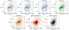 |
Fig. 1. Multi-wavelength data for the galaxy VC875, shown at their native resolutions. From left to right: The first row presents HST/ACS F814W (rest-frame 145 nm), JWST/NIRCam F115W (207 nm), F150W (270 nm), and F277W (499 nm). The second row shows JWST/F444W (800 nm), ALMA dust continuum emission around 157 μm, and ALMA [CII] 158 μm emission. The contours are those of the ALMA [CII] line emission maps starting from 3σ increasing by steps of 2σ. Ellipses in the bottom left corners represent the central lobe of the PSF for HST and JWST images, and the synthesised beam for ALMA images. |
2.3. Homogenisation of the resolution
To perform accurate pixel-by-pixel comparisons across all available bands for our SED modelling process, we need to ensure that the information contained within each pixel corresponds to the same region of the sky, for all observational bands. This consistency is crucial for deriving reliable physical properties from multi-wavelength data. Therefore, we performed point spread function (PSF) homogenisation across all bands to match their resolutions. We used the ALMA beam as the target resolution since it is the coarsest in our sample. The HST and JWST PSFs central lobes were modelled with 2D Gaussian functions to retrieve their full width at half maximum and maximumintensity.
Cleaned synthesised ALMA beams models were created based on dust continuum map header parameters, assuming a 2D elliptical Gaussian shape. Convolution kernels were generated to transform HST and JWST PSFs to match the target ALMA beam taking into account different grid orientations, pixel scales, and normalisation conventions. We re-projected HST and JWST convolved images onto the ALMA astrometric grid using the reproject_interp module from the Python package reproject1, ensuring consistent pixel sampling and astrometric alignment across all bands. Applying the procedure to a point-like source with unit flux in HST/JWST native resolution, we find the reconstructed average flux to be 2.6% lower than the expected peak value of unity across the different filters. The missing flux likely resides in the secondary lobes not taken into account, and we consider this effect to be negligible compared to our overall flux calibration uncertainties.
Figure 2 shows the effect of the resolution homogenisation of the JWST/NIRCam F150W filter in the case of VC875. The complete set of homogenised observations for this source is found in Fig. A.1. As a result of this resolution homogenisation, we achieve an average beam size of 0.3″ (∼2 kpc) across the sample. Although the pixel scale is ∼0.2 kpc, the physical information is correlated on the scale of the beam. We take into account these correlations induced by our resolution homogenisation in our analysis of the [CII]-SFR relation (see Sect. 3.3).
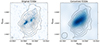 |
Fig. 2. Native resolution image of VC875 (left panel) and the homogenised version matching the ALMA resolution (right panel) for the JWST/NIRCam F150W filter. The contours and ellipses are the same as in Fig. 1. |
2.4. Photometric and line flux unit conversion
To prepare the data for SED modelling, we converted all photometric data to micro janskys per beam, and ALMA dust continuum emission flux to dust luminosity. Here ‘beam’ refers to the synthesised ALMA beam, not the PSF of each instrument. Expressing fluxes per beam ensures that the measurements are referenced to the area over which the instrument is sensitive. The dust luminosity, LIR (W beam−1), was calculated from the monochromatic flux, Sν (Jy  ), using
 (1)
(1)
where νem is the rest-frame emission frequency at 158 microns (hertz), DL is the luminosity distance (metres), and z is the redshift. The factor 10−26 converts janskys to watts per square metre per hertz, while the 1/(1 + z) term accounts for cosmological redshift. We adopted the empirical conversion factor of  from Khusanova et al. (2021) to convert the
  rest-frame monochromatic luminosity into the total infrared luminosity,
  . This value corresponds to the calibration for the redshift bin
  and is directly applicable to our sample, which predominantly lies within this range. The other sources are in the 5 < z < 6 bin, in which Khusanova et al. (2021) measured a conversion factor of
  . Since the two values are compatible with no redshift dependence, we use the more accurate value found at 4 < z < 5 for the full sample. Both factors were calibrated using stacked SEDs. A compilation of SED templates from the literature was fitted to these SEDs and only the good fits were kept (reduced χ2 < 1.5). The conversion factor was then estimated using the mean and dispersion of these templates. The typical dust temperatures corresponding to these stacked SEDs are
  at z ∼ 4.5 and
  at z ∼ 5.5 for galaxies with
  (see Appendix A of Khusanova et al. 2021). We note that adopting a constant conversion factor assumes a uniform dust temperature across the sample, and variations could introduce systematic effects on
  and thus
  estimates (Faisst et al. 2017; Cochrane et al. 2022). We include this IR dust luminosity in the SED modelling process as a constraint on dust attenuation models (see Sect. 3.1).
The [CII] surface brightness (Σ[CII] in solar luminosities per square kiloparsec) was derived from the [CII] moment-0 map (m[CII] in janskys kilometre per second per beam) using
![Mathematical equation: $$ \begin{aligned} \Sigma _{\mathrm{[CII]} } = \frac{m_\mathrm{[CII]} }{D_\mathrm{A} ^2\, \Omega _{\mathrm{Beam} }} \, \left(1.04 \times 10^{-3}\,\frac{\mathrm{L} _\odot }{\mathrm{GHz\,Mpc ^2\, \mathrm {Jy\,km\,s}^{-1}}} \right) \, D_\mathrm{L} ^2 \, \nu _{\mathrm{obs} }, \end{aligned} $$](/articles/aa/full_html/2025/10/aa56140-25/aa56140-25-eq14.gif) (2)
(2)
where DA2 ΩBeam is the physical area associated with the synthesised beam, defined by DA, the angular distance (in kiloparsecs), and ΩBeam, the solid angle of the beam. The remaining factors correspond to the conversion from line flux to luminosity (Solomon et al. 1992), where DL is the luminosity distance (in megaparsecs) and νobs the observed frequency (in gigahertz).
2.5. Uncertainty estimation
For HST and JWST images, we incorporated the convolution systematic error from Section 2.3. In addition, we applied a relative uncertainty of 3% to JWST images to account for potential calibration uncertainties (Gordon et al. 2018). The conversion from continuum flux to LIR relies on an empirical factor of 0.13 ± 0.02, which introduces a relative systematic uncertainty of approximately 15% (0.02/0.13) to the derived LIR values in our continuum images. For images lacking error maps (HST data and LIR), we assumed white noise at the native resolution and estimated the measurement uncertainty using the standard deviation of the noise in the convolved then reprojected image. For Σ[CII], we used the pixel-by-pixel error maps provided by the CRISTAL team.
JWST maps are provided with their associated error maps. We produced variance maps of the resolution-homogenised maps (in janskys per pixel) by convolving the noise variance map (error map squared) by the kernel:
 (3)
(3)
where σconv2 and σpixel2 are the noise variance of the convolved and original maps, respectively, and K is the homogenisation kernel. We compared the results with the standard deviation of the noise in an empty area of the homogenised map, and we found a small excess, likely due to a small contribution from correlated noise already present in the original maps and not taken into account by our computation. This excess remains negligible for the short-wavelength filters (less than 6% for F115W and F150W), but becomes increasingly significant at longer wavelengths, reaching up to 14% for F277W and F444W. We thus applied a scaling factor (1–1.14, depending on the source and band) to the resolution-homogenised error maps to correct for this effect.
To account for this error budget in our analysis, we generated 100 perturbed realisations of each image. This process involves adding white noise with a standard deviation equal to the measured pixel-level noise at the native resolution of each image, followed by the application of systematic errors. The HST and JWST perturbed images were subsequently convolved. This method accounts for the non-independence of the pixels from spatially correlated noise and the smoothing of the maps.
3. Methods
3.1. Resolved SED fitting
Our primary objective is to derive the SFR along each line of sight for the galaxies in our sample by combining multi-wavelength observations. At a spatial resolution of 2 kpc, the use of an energy-conserving SED modelling code is justified, as the energy balance assumption-where UV/optical energy absorbed by dust is re-emitted in the IR-remains physically meaningful at this scale (e.g. Boquien et al. 2015).
To this end, we used CIGALE, a versatile Python tool capable of modelling galaxy emission from X-ray to radio wavelengths (Boquien et al. 2019). Its modular design allows for the inclusion of diverse SFHs, dust attenuation laws, and emission line models tailored to specific scientific objectives. CIGALE uses a Bayesian approach to perform parameter estimation, generating a large library of theoretical SEDs based on user-defined models. Observed data were then compared to these models, and posterior probability distributions were calculated for each parameter. This Bayesian framework ensures that uncertainties and degeneracies between parameters are properly propagated into the resulting parameter estimates.
In this section, we present the SED modelling parameters used for our analysis. We followed Boquien et al. (2022), who analysed integrated measurements of the ALPINE galaxies (our parent sample), and Buat et al. (2019), who focused on dust-rich galaxies at z ∼ 2. We refer the reader to those works for a comprehensive discussion of parameter choices. Our focus here is to detail the differences. A summary of our parameters is given in Table B.1.
We adopted delayed SFH model with an additional recent variation, as is described by Ciesla et al. (2017). In this framework, star formation begins after an initial delay corresponding to the time between the Big Bang and the onset of the first stars (here set to 250 Myr). The main stellar population forms according to a delayed SFH, which rises linearly from the onset, peaks at a characteristic timescale, and then declines exponentially. To capture recent deviations from this smooth evolution, we introduced a modification to the SFR at a specified time in the recent past. The SFH is thus expressed as
 (4)
(4)
where t is the time since the onset of star formation, τ is the SFH timescale, tvar is the time since the onset of the recent SFR variation, and rSFR is the factor by which the SFR is increased or decreased. This approach provides flexibility to model both the overall stellar mass assembly and any recent changes in star formation activity that a simple delayed SFH model would not account for.
For all sources, we adopted the two-component dust attenuation model of Charlot & Fall (2000). This choice is motivated by its physical basis and agreement with radiative transfer predictions, allowing it to be applicable across the full range of dust attenuation, from weakly to highly obscured regions. While the modified Calzetti et al. (1994, 2000) relation (Noll et al. 2009) is often used for star-forming galaxies, it is less appropriate for low attenuation or highly obscured systems (e.g. Boquien et al. 2022), and allowing its slope parameter (δ) to vary could lead to overfitting given our limited number of photometric bands. Although for most of our sample there are no significant differences between the two models (as is illustrated by VC875; see Appendix C), the Charlot & Fall (2000) law provides a substantially better agreement between SFR estimators for CRISTAL_24 (see Fig. C.2), further consolidating our choice of attenuation law.
We also evaluated the impact of including the ALMA-derived total infrared luminosity (LIR, computed from the 158 μm continuum in Sect. 2.4) as a dust luminosity constraint in our SED modelling. We find that omitting this constraint causes the models to systematically overestimate the SFR compared to estimates from combined UV and far-IR data. This finding is consistent with Li et al. (2024), who reported a similar discrepancy in an overlapping sample. Their analysis, using region-averaged measurements with the magphys (da Cunha & Charlot 2011) SED fitting code, likewise highlights the necessity of the dust luminosity constraint in SED modelling. Our results, derived from a pixel-based CIGALE approach, reinforce this conclusion.
In Appendix C, we discuss our final modelling choices in detail, using the galaxy VC875 as a case study. These choices include the dust luminosity constraint, the adopted dust attenuation law, and the treatment of recent star formation episodes. A similar analysis was performed for all other sources in thesample.
To ensure robust measurements, we used only pixels with Σ[CII] ≥ 5σ[CII] and S/N≥2 in at least three bands. The latter cut, applied to the data used for SFR estimates, excludes only about 6% of pixels that passed the L[CII] threshold, confirming that our selection is primarily driven by [CII] detectability. This ensures the robustness of the [CII] measurements, while minimising biases in the inferred SFR distribution.
The SFR uncertainties were estimated from the 16th, 50th, and 84th percentiles of the log(SFR) distributions obtained via resampling noise realisations (see Sect. 2.5). This approach accounts for pixel correlations introduced by resolution-matching. It avoids biases from assuming Gaussian errors, as the SFR distributions are typically skewed.
Figure 3 presents the maps of stellar mass, SFR, mass-weighted age, and FUV attenuation for VC875, derived from SED modelling after applying all pixel selection criteria. These spatially resolved maps help to verify the reliability of our results by revealing whether parameters vary smoothly and align with the galaxy’s morphology. These maps also make it easier to search for modelling artefacts, such as abrupt discontinuities or parameter saturation. This enables a direct comparison of physical property distributions with features seen at other wavelengths or in simulations, providing a useful check on our assumptions. Across the sample, we find that stellar mass and SFR peaks are generally aligned. In contrast, the mass-weighted ages and FUV attenuation exhibit more complex and asymmetric patterns (see Appendix F).
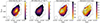 |
Fig. 3. Example of physical parameters maps obtained with the CIGALE SED modelling for VC875. From left to right: Stellar mass surface density (solar masses per square kiloparsec), SFR surface density averaged over 10 million years (solar masses per year per square kiloparsec), mass-weighted age (million years), and attenuation in the FUV rest frame (magnitudes). The contours are those of the [CII] luminosity map, starting at 3σ and increasing by steps of 2σ. The ellipse in the bottom left of each panel represent the synthesised ALMA beam. The maps are shown for the pixels having L[CII] ≥ 5σ[CII] and S/N ≥ 2 in at least three bands. |
3.2. Fitting the SFR-[CII] relation
To study the relationship between the SFR obtained by the SED modelling and the [CII] luminosity, we parametrised this relation as a power law with an intrinsic scatter that accounts for the variations in the physical conditions:
![Mathematical equation: $$ \begin{aligned} \log _{10}(\Sigma _\mathrm {SFR} ) = \log _{10}(C) + \beta \log _{10}(\Sigma _\mathrm{[CII]} ) \pm \sigma _{\rm i}, \end{aligned} $$](/articles/aa/full_html/2025/10/aa56140-25/aa56140-25-eq17.gif) (5)
(5)
where β, C, Σ[CII], ΣSFR, and σi are the slope, the normalisation constant, the [CII] surface brightness, the SFR surface density, and the intrinsic scatter, respectively.
To estimate the slope and scatter of the [CII]-SFR relation, we used a Bayesian fit relying on a maximum likelihood estimator. We constructed a likelihood that properly accounts for both normal distribution of [CII] maps error and log-normal nature of SFR distributions, but also estimates the intrinsic scatter. To mitigate potential degeneracies between the normalisation factor and the slope when fitting the data, we introduced a normalised [CII] surface brightness:
 (6)
(6)
where gk represents the [CII] surface brightness measurement for each data point, k, and the subscript norm indicate normalisation by the reference value, g0. The parameter g0 is a fixed normalisation pivot introduced to reduce the degeneracies between the slope, β, and the normalisation constant, C, and was set to the median [CII] surface brightness in our sample, (log10(g0) = 7.5 L⊙ kpc−2). The slope, β, is independent of the choice of g0, while the normalisation constant, C, is expressed relative to this pivot (denoted C0). The sample log10 gk values ranges from 6.89 to 8.51, with an interquartile range of 7.23 to 7.92, confirming the representativeness of this choice.
Next, we addressed the statistical treatment of our data. For each data point, k, in the [CII]-SFR plane, we considered the normalised [CII] surface brightness (gk, n) and SFR surface density (sk). To account for the uncertainties in the [CII] measurements, we modelled the true value gt of a given gk, n measurement as a normal distribution with standard deviation σg, k. This uncertainty is incorporated into the likelihood through marginalisation over the gt parameter.
Since the SFR estimates followed a log-normal distribution, we worked with the log-quantity, denoted as yk = ln(sk), which then followed a normal distribution. The mean of this distribution is given by μ = ln(C0)+βln(gt). Finally, the standard deviation of this new distribution, σT, accounts for both the SFR estimate error and the intrinsic scatter of the relation
 (7)
(7)
where σy, k represents the SFR estimate error for a pixel, k, computed from the yk = ln(sk) distribution and σi, the intrinsic scatter of the SFR-[CII] relation.
With this description, the likelihood for a given pixel is expressed as
 (8)
(8)
The first term in the likelihood, p(yk, σy, k|gt, C0, β, σi), represents the KS relation and its associated uncertainties, while the second term, p(gt|gk, n, σg, k), accounts for the observational uncertainty on the [CII] surface brightness measurements.
By marginalising over gt, we propagated these uncertainties into our parameter estimation. The marginalisation was performed numerically by integrating on the gk, n ± 5(σg, k) range spanned by a grid of 1000 linearly spaced values. This covers 99.99994% of the probability mass for a normal distribution, and thus captures nearly the entire range of plausible true [CII] surface brightness values. To estimate the model parameters, we maximised the total log-likelihood across all data points. This is equivalent to minimising the following negative log-likelihood:
 (9)
(9)
Physical constraints enforcing positivity (C > 0, σi > 0) were imposed via flat, uniform priors restricted to the physically meaningful domain of positive values. Parameter optimisation was performed using L-BFGS-B (from scipy.minimize function), a boundary-aware algorithm specifically designed for constrained optimisation.
To assess potential biases in this fitting methodology, we performed an end-to-end numerical simulation that replicates the full observational chain, from mock source generation, noise injection, and resolution homogenisation to the inference of the physical relation parameters. This revealed no systematic parameter estimation biases on a simulated population similar to our sample (see Appendix D). However, when considering individual galaxies with a limited amount of independent data points, we obtained unreliable results, highlighting the necessity of combining multiple objects to recover the proper physical relation.
3.3. Uncertainty quantification
To evaluate the robustness of our results and quantify uncertainties in the model parameters, we implemented a systematic resampling strategy. This approach used the ensemble of the 100 perturbed [CII] maps per source in our sample and their corresponding SFR estimates (derived in Sects. 2.5 and 3.1), combined with the unperturbed dataset. We investigated three distinct methods to disentangle sources of uncertainty, applying each method 1000 times to generate robust parameter distributions. The first one, called source bootstrapping, consisted of selecting 13 sources with replacement of the original noise realisation. This was used to test the sample representativeness. The second one, called noise sampling, selected the original 13 sources but with a random noise realisation, enabling an assessment of the impact of observational noise. Finally, we performed a hybrid resampling by selecting 13 sources randomly as well as a random noise realisation to combine both effects. For the last two methods, we accounted for the additional noise introduced by the resampling process by using  times larger uncertainties in our fitting procedure.
In addition to our primary resampling methods, we explored alternative fitting methods. Details of these supplementary analyses, including linmix2 Bayesian regression and Markov chain Monte Carlo (MCMC) techniques, are presented in Appendix E. The results of these secondary approaches are summarised in Table 2 for direct comparison with the primary resampling methods, and are discussed in Sect. 4.1.
4. Results
4.1. Resolved SFR-[CII] relation
We began by fitting the resolved [CII]–SFR surface densities relation for our z ∼ 5 galaxy sample using our tailored likelihood-based fitting routine, applied to the original noise realisation of all 13 galaxies. This yielded a best-fit power-law model with log(C0) = 0.30, β = 0.87, and σi = 0.19 dex. At this stage, we just derived the best fit, and formal uncertainties were not directly obtained. To assess the precision of these results, we compared them to those obtained with our primary resampling strategies. Using population bootstrapping, we found parameter estimates that are consistent with the baseline fit and that show uniform relative uncertainties of ∼15% for all parameters:  ,
,  , and
, and  . These uncertainties remain stable across 1000 resamplings, despite the modest sample size (N = 13), indicating that the measured relation is not dominated by individual outliers. In contrast, the noise sampling approach yields a slightly flatter slope (
 ) and a marginally higher intrinsic scatter (
 ). The hybrid resampling method shows a combination of both trends (
 ). The largest error bars on the slope arise from source bootstrapping, highlighting the influence of sample selection, whereas noise resampling yields lower slope values. Importantly, the intrinsic scatter remains remarkably stable across all methods, providing a reliable measure of how tightly [CII] emission traces star formation in our sample. These results are summarised in Table 2.
Figure 4 shows the relation between SFR surface density and [CII] surface brightness for our z ∼ 5 sample. We present the best-fit model derived from our tailored likelihood-based approach for both the original sample and theregion-averaged pairs following the B23 methodology. For comparison, we also plot the relation from Herrera-Camus et al. (2015), which is based on spatially resolved measurements at ∼0.2–1.5 kpc scales for 46 nearby galaxies (d < 30 Mpc). While the majority of our z ∼ 5 sample lies above their local [CII]–SFR relation, our resolved analysis yields a shallower slope and similar intrinsic scatter compared to the lower-redshift study of Herrera-Camus et al. (β = 1.13 ± 0.01, σi = 0.21 dex, reported without uncertainty). In addition to the redshift difference, the parameter space covered by the two samples is very different: the Herrera-Camus et al. (2015) sample spans 4.4 < logΣ[CII] (L⊙ kpc−2) < 6.5, whereas our sample covers 6.8 < logΣ[CII] < 8.6. This difference likely contributes to the observed slope discrepancy as it may reflect the evolution in ISM physical conditions across cosmic time, such as increased turbulence, lower metallicity, or changes in ISM structure at high redshift, yielding different dynamical range in Σ[CII] as well as ΣSFR. We emphasise that methodological differences also play a critical role, especially on observation-based studies. For instance, Herrera-Camus et al. (2015) employed a least-squares bisector, which neglects pixel covariance. In contrast, our tailored approach explicitly accounts for pixel covariance and highlights the sensitivity of the slope estimate to this effect, as is demonstrated by the various tests conducted below.
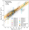 |
Fig. 4. Resolved [CII]-SFR relation for galaxies at z ∼ 5. The grey contours show the individual pixel distribution for the whole sample. Each pair of coloured points represents a high- and low-[CII] density average region for each galaxy of the sample following B23 methodology. The orange line and shaded region shows our best-fit power-law model from the tailored likelihood-based approach with the parameters in the top left corner (where log10(C0) is the value at g0 = 107.5 L⊙ kpc−2). The dashed black line presents the extrapolation of the relation derived from a spatially resolved sample of 46 nearby galaxies by Herrera-Camus et al. (2015). We represented the typical errors bars for the individual pixels across the sample with three black squares. |
We also explored alternative fitting methods to further validate our findings, which are presented in Appendix E. A MCMC analysis of the unperturbed dataset reproduces the best-fit parameters of the baseline fit, but initially yields unrealistically narrow error bars. For example, the MCMC approach yields an intrinsic scatter of σi = 0.19 ± 0.002, showing error bars an order of magnitude smaller than uncertainties obtained via hybrid resampling (∼0.03). This discrepancy likely arises from neglected correlations in the data. To correct for this, we used the likelihood normalised by half the number of pixels per beam, resulting in more realistic uncertainties that closely match those from the hybrid resampling approach (e.g. σi = 0.20 ± 0.02). Using the linmix Bayesian regression method on the original dataset produces a slightly steeper slope ({β = 0.92 ± 0.02) and comparable intrinsic scatter (σi = 0.18 ± 0.04 dex), again with very narrow uncertainties. To mitigate the impact of pixel covariance, we also applied linmix to region-averaged points following the B23 methodology that consists of averaging the SFR and Σ[CII] measurements over large regions to obtain a sufficiently elevated signal-to-noise ratio and by construction gives a pair of points per galaxy corresponding to the low and high regime of [CII] surface brightness (pairs of points in Fig. 4 and Fig. 5). This approach yields a steeper slope than the pixel-based fit (β = 1.02 ± 0.12) but a smaller and poorly constrained scatter (σi = 0.06 ± 0.08 dex).
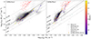 |
Fig. 5. Kennicutt-Schmidt relation using the α[CII] conversion factor (left) and the W[CII] version (right). The grey contours show the distribution of individual pixel measurements across the entire sample; the pair of points are the B23 region averages for individual galaxies, colour-coded by redshift. The dashed grey lines show constant gas depletion time. The dashed black line represents the Wang et al. (2022) KS relation for local Universe and high-redshift main-sequence galaxies. We show CO measurements of the global KS relation from the low-z COLD GASS sample (Saintonge et al. 2012, crosses) and at redshifts up to z ∼ 2.5 from the PHIBBS (Tacconi et al. 2013, plus signs) and PHIBBS2 (Freundlich et al. 2019, three-branch stars) programmes, together with a resolved z = 2.6 lensed starburst (Sharon et al. 2013, red points). |
The MCMC and resampling methods yield parameter estimates that agree within ∼1σ, demonstrating the robustness of our resolved analysis. In contrast, the linmix method yields a slightly higher slope and a poorly constrained intrinsic scatter, indicating a mild tension with the other primary approaches. These comparisons highlight the importance of properly accounting for pixel covariance, as methods that neglect this effect can underestimate uncertainties or fail to reliably constrain the intrinsic scatter.
Because of the limitations of our model when applied on a per-galaxy basis – that is, with restricted Σ[CII] dynamic ranges (see Sect. 3.2) – we were unable to recover resolved [CII]–SFR relations per galaxy. We therefore adopted the linmix method for simplicity, acknowledging that it does not properly account for pixel correlations. This method yields an average slope of 1.27, which is consistent with the mean value of 1.21 derived from Li et al. (2024) using spatially bin-averaged measurements on the same ALPINE-CRISTAL sample. As this value is manually measured from their Fig. 12, no formal uncertainty is provided. This agreement suggests that, despite the methodological differences and the limited dynamic range within single galaxies, the underlying scaling relation inferred from spatially resolved data remains broadly compatible with results based on coarser spatial binning.
Our results offer a valuable comparison to the theoretical predictions of Ferrara et al. (2019), who used spatially resolved models to investigate the [CII]-SFR relation within galaxies. Their work explored how local ISM conditions (e.g. density, metallicity) shape the resolved ![Mathematical equation: $ \rm \Sigma_{[CII]}-\Sigma_{SFR} $](/articles/aa/full_html/2025/10/aa56140-25/aa56140-25-eq44.gif) relation, finding that it steepens at high surface densities due to
relation, finding that it steepens at high surface densities due to ![Mathematical equation: $ \rm \Sigma_{[CII]} $](/articles/aa/full_html/2025/10/aa56140-25/aa56140-25-eq45.gif) saturation. We observe a similar trend on local scales, with the mean slope within individual galaxies aligning with their predictions. However, our relation is significantly shallower for the population as a whole, confirming that this steepening is a local effect. This contrast highlights the critical role of spatial scale in interpreting the [CII]-SFR relation. Furthermore, it underscores the need for both local and population-wide perspectives to fully understand the diverse ISM conditions at high redshift.
saturation. We observe a similar trend on local scales, with the mean slope within individual galaxies aligning with their predictions. However, our relation is significantly shallower for the population as a whole, confirming that this steepening is a local effect. This contrast highlights the critical role of spatial scale in interpreting the [CII]-SFR relation. Furthermore, it underscores the need for both local and population-wide perspectives to fully understand the diverse ISM conditions at high redshift.
4.2. [CII]-to-gas conversion factors
To estimate the gas mass, we first used the prescription of Zanella et al. (2018): the conversion factor is constant with a value of α[CII] = 31 M⊙ L⊙−1, and the gas mass surface density was derived as
![Mathematical equation: $$ \begin{aligned} \Sigma _\mathrm{gas} = \alpha _\mathrm{[CII]} \,\Sigma _\mathrm{[CII]} . \end{aligned} $$](/articles/aa/full_html/2025/10/aa56140-25/aa56140-25-eq46.gif) (10)
(10)
It is well established that [CII] emission can originate from multiple ISM phases, primarily PDRs and molecular gas, yet the contributions of these phases to the total [CII] luminosity remain debated and are sensitive to local ISM conditions. Consequently, the dominant gas phase traced by [CII] can vary across different environments, particularly at high redshift where ISM properties often diverge from those in local galaxies. This diversity has a direct impact on the appropriate [CII]-to-gas conversion factor (e.g. Madden et al. 2020; Vizgan et al. 2022). Recent theoretical work reinforces this perspective: Vallini et al. (2025), using galaxies from the SERRA cosmological zoom-in simulation (Pallottini et al. 2022), derive a relation varying with the [CII] surface brightness:
![Mathematical equation: $$ \begin{aligned} \log W_{\mathrm{[CII]} } = -0.506 \, \log \Sigma _\mathrm{[CII]} + 4.933, \end{aligned} $$](/articles/aa/full_html/2025/10/aa56140-25/aa56140-25-eq47.gif) (11)
(11)
where the W[CII] notation is used to express the resolved, surface-brightness-dependent conversion factor, in contrast to the global α[CII] value. This relation exhibits a typical 1σ dispersion of 0.4 dex. The dependence on Σ[CII] encapsulates the expectation that brighter [CII] regions are denser and more metal-enriched, two conditions that drive higher [CII] emission efficiency per unit gas mass. Across the ![Mathematical equation: $ \rm 6.8 < \log \Sigma_{[CII]}\,(L_{\odot}\,kpc^{-2}) < 8.6 $](/articles/aa/full_html/2025/10/aa56140-25/aa56140-25-eq48.gif) range probed in our sample, W[CII] varies from
range probed in our sample, W[CII] varies from  in the faintest regions down to
  in the brightest regions. This prescription can therefore lead to a steeper slope in the KS relation derived from [CII], particularly at high surface densities. It is important to note that the conversion from Vallini et al. (2025) yields a relation computed for the total cold gas content. This total content encompasses both atomic and molecular phases, thereby accounting for the outer layers of PDRs and the fully molecular clumps within clouds.
To explore the implications of this conversion factor on our interpretation of [CII]-based observations, we included it in our analysis. Using the W[CII] formula from Eq. (11) in place of α[CII] in Eq. (10) yields
![Mathematical equation: $$ \begin{aligned} \Sigma _{\mathrm{[CII]} } \propto \Sigma _{\mathrm{gas} }^{1/0.494}. \end{aligned} $$](/articles/aa/full_html/2025/10/aa56140-25/aa56140-25-eq51.gif) (12)
(12)
Substituting this relation into Eq. 5 gives
![Mathematical equation: $$ \begin{aligned} \Sigma _{\mathrm{SFR} } \propto \Sigma ^\beta _\mathrm{[CII]} \text{ and} \text{ thus} \Sigma _{\mathrm{SFR} } \propto \Sigma _{\mathrm{gas} }^{\beta /0.494}. \end{aligned} $$](/articles/aa/full_html/2025/10/aa56140-25/aa56140-25-eq52.gif) (13)
(13)
This implies that for a given slope, β, of the SFR–[CII] relation, the slope of the SFR–gas relation is expected to be approximately twice as steep. In contrast, the constant α[CII] prescription leaves the slope, β, unaffected.
4.3. Impact on the Kennicutt–Schmidt relation
Figure 5 presents the resolved KS relation for our z ∼ 5 sample, contrasting two [CII]-to-gas conversion prescriptions. The left panel adopts the constant α[CII] from Zanella et al. (2018), and the right applies the surface-brightness-dependent W[CII] from Vallini et al. (2025). In both cases, we overlay a set of reference data from CO-based global KS relations from the low-redshift COLD GASS sample (Saintonge et al. 2012), as well as higher-redshift measurements from PHIBBS (Tacconi et al. 2013) and PHIBBS2 (Freundlich et al. 2019). The resolved z = 2.6 lensed-starburst of Sharon et al. (2013) is also shown, providing a benchmark for extreme star-forming environments. The dashed black line in both panels represents the KS relation for local and high-redshift main-sequence galaxies from Wang et al. (2022). Due to the substantial dispersion inherent to both conversion factor prescriptions, our fitting methodology cannot robustly constrain the intrinsic scatter of the relation. As such, the following discussion provides a qualitative assessment of the observed trends, and reported parameter values should be interpreted with caution.
When adopting a constant α[CII], our sample is compatible with the Wang et al. (2022) results, despite a small slope difference (β = 1.13 ± 0.09 for Wang et al. 2022, β = 0.87 ± 0.06 in this work). The data align with constant gas depletion times of ∼0.5 − 1 Gyr, extending the locus of the low- and intermediate-redshift CO-based studies (Saintonge et al. 2012; Tacconi et al. 2013; Freundlich et al. 2019) to higher gas and SFR surface densities. Interestingly, these are ∼2 − 3 times shorter than those usually found for local star-forming spirals at the similar physical scales using CO-based H2 tracers (e.g Schruba et al. 2011; Leroy et al. 2023; Villanueva et al. 2021, 2024). Within individual galaxies, we observe moderate internal variations, with denser regions showing shorter depletion times, but no evidence of extreme starburst-like behaviour, with depletion times above 0.25 Gyr throughout.
Applying the W[CII] prescription fundamentally alters the picture. The derived slope steepens to β = 1.75 ± 0.14, and the sample bridges the gap between the low-redshift CO-based locus and the regime occupied by the z = 2.6 starburst of Sharon et al. (2013). Several regions within our galaxies, particularly in CRISTAL_09, CRISTAL_13, and CRISTAL_24, overlap with these resolved starburst measurements. This change is accompanied by a pronounced decrease in depletion times across the most [CII]-emitting regions, with values reaching as low as 0.1 Gyr, characteristic of starburst systems, in the brightest [CII] regions. Importantly, this shift towards shorter depletion times is not restricted to isolated, compact star-forming regions, but is observed globally across the galaxies. While increasing spatial resolution is generally expected to broaden the dynamic range of depletion times and reveal localised starburst-like environments, we do not observe such a trend here. Instead, the W[CII] conversion produces a systematic reduction in depletion times throughout all regions, compressing the inferred gas mass range. This raises the possibility that, under certain conversion prescriptions, main-sequence galaxies could exhibit global properties reminiscent of starbursts, challenging the classical separation between main-sequence and starburst systems.
Recent results from the THESAN-ZOOM simulations (Shen et al. 2025) show a similar trend towards shorter depletion timescales for Σgas > 100 M⊙ pc−2. In their sample of galaxies with stellar masses up to 1011 M⊙ at z ∼ 3 and 109.6 M⊙ at z ∼ 5, resolved depletion times for neutral gas (HI+H2) can reach as low as 0.1 Gyr in the densest regions (see their Fig. 8). This is consistent with the short depletion times inferred in our analysis.
Additionally, we colour-code our sample by redshift in Figure 5 and find no clear redshift dependence of the relative position of the galaxies within the KS plane. Under the constant ![Mathematical equation: $ \rm \alpha_{[CII]} = 31\,M_{\odot}\,L_{\odot}^{-1} $](/articles/aa/full_html/2025/10/aa56140-25/aa56140-25-eq53.gif) , high-redshift main-sequence galaxies exhibit KS behaviour remarkably similar to their low-redshift counterparts, as traced by CO. In contrast, the W[CII] approach reveals a population of short-depletion-time regions that bridge the loci of main-sequence galaxies and starburst regimes, demonstrating the strong sensitivity of inferred gas properties, and thus depletion time estimates, to the adopted [CII]-to-gas calibration. As a result, our ability to confidently study the KS relation at high redshift is compromised.
, high-redshift main-sequence galaxies exhibit KS behaviour remarkably similar to their low-redshift counterparts, as traced by CO. In contrast, the W[CII] approach reveals a population of short-depletion-time regions that bridge the loci of main-sequence galaxies and starburst regimes, demonstrating the strong sensitivity of inferred gas properties, and thus depletion time estimates, to the adopted [CII]-to-gas calibration. As a result, our ability to confidently study the KS relation at high redshift is compromised.
5. Discussion
To further investigate the possible physical drivers of the derived KS relations, we constructed a diagnostic plot shown in Fig. 6 encoding AGN activity, stellar mass, and merger status for our sample by changing symbol type, size, and colour, respectively. The AGN identification follows Ren et al. (in prep.), while the merger status is classified according to Herrera-Camus et al. (2025). Additionally, environmental classification distinguishes between field galaxies and those residing in the z ∼ 4.57 protocluster structure (CRISTAL_13, CRISTAL_15, and VC875; see Lemaux et al. 2018; Staab et al. 2024). Visual inspection of the KS diagram reveals no clear systematic offset or trend associated with AGN presence, merger stage, stellar mass, or environment across the KS plane. Within the dynamic range probed by our study, none of these properties seems to have a significant impact on the star formation. Nevertheless, we caution that the uncertainties and limited sample size may reduce sensitivity to subtle or systematic effects.
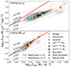 |
Fig. 6. Similar to Fig. 5. This time, symbols indicate integrated measurements for individual galaxies, colour-coded by interaction state: light blue for major mergers, light yellow for interacting systems, and orange for isolated galaxies, following the classification of Herrera-Camus et al. (2025). Symbol size encodes the total stellar mass and symbol shape denotes AGN identification: circles for non-AGNs, squares for AGN candidates, and triangles for robust AGNs as per Ren et al. (in prep.). The solid blue line shows the z = 4 relation from Kraljic et al. (2024), based on the 25% most massive galaxies in the NewHorizon simulation, while the solid red line indicates the NewCluster analogue (Han et al. 2025). Both relations are plotted over their effective gas mass ranges for direct comparison with our sample. |
We also show KS relations for the most massive 25% of galaxies at z = 4 in both the NewHorizon (Dubois et al. 2021; Kraljic et al. 2024) and NewCluster (Han et al. 2025) simulations, presented in their respective effective gas surface density regimes. The main difference between the two simulations is environmental: NewCluster targets a high-density proto-cluster region, while NewHorizon samples an average-density field. Both use similar physical models for star formation and feedback. In the constant α[CII] case, our observed sample aligns well with predictions from the New Horizon simulation, though this simulation primarily probes lower stellar masses (108.0 − 9.5 M⊙) than our galaxies (109.5 − 10.6 M⊙). In comparison, the most massive 25% of galaxies in the NewCluster simulation span a similar stellar mass range (M* = 109.5 − 10.5 M⊙). We find that employing a density-dependent W[CII] conversion factor aligns with their results. This compatibility could support the fact that the stellar mass affects the slope of the KS relation for high-redshift galaxies, specifically a steepening of the slope as the total stellar mass of the population increases, as is hinted at by the z = 2 − 3 relations presented in Kraljic et al. (2024).
The contrasting behaviours obtained assuming the two different gas-conversion prescriptions, and their respective alignments with different simulations, show the need for reliable [CII]-to-gas mass conversion methods that account for the ISM conditions prevailing at a given redshift and in a specific population of galaxies. Even though we cannot fully exclude it at this stage, the lack of correlation with AGN or merger status further points to intrinsic ISM properties, such as density, turbulence, and metallicity, as the dominant factors shaping the [CII]-to-gas calibration and, by extension, the inferred star formation law.
These results highlight the limitations of adopting a universal [CII]-to-gas conversion factor and motivate the development of physically motivated, simulation-calibrated or locally calibrated prescriptions that account for galaxy mass, environment, and ISM state. Joint analysis of resolved observations and simulations, as is demonstrated here, is essential for building an accurate picture of the star formation mechanisms in the high-redshift Universe.
6. Conclusions
We present a spatially resolved analysis of the [CII]–SFR and KS relations in a sample of 13 main-sequence galaxies at redshifts of 4 < z < 6, combining ALMA, JWST, and HST data. Our pixel-by-pixel SED modelling approach applied to resolution-homogenised multi-wavelength datasets allows us to probe the physical conditions of star formation down to correlated kiloparsec scales in the early Universe.
We have developed a new comprehensive statistical framework that explicitly accounts for correlated noise and pixel covariance introduced by resolution homogenisation. By combining noise sampling, source bootstrapping, and hybrid resampling techniques, we reliably estimate the intrinsic scatter and slope of the spatially resolved [CII]-SFR relations. Comparison with classical fitting methods demonstrates that neglecting pixel correlations leads to underestimated uncertainties. This shows the relevance of our approach for robust parameter inference.
Our analysis reveals that the resolved [CII]–SFR relation exhibits a slope of 0.87 ± 0.15 and an intrinsic scatter of 0.19 ± 0.03 dex. These values are both shallower and tighter than those reported in many studies of the local Universe, suggesting a possible saturation of the SFR emission at high [CII] surface densities, population wise, while confirming a strong correlation between [CII] and SFR at z ∼ 5. This tight relation supports the use of [CII] as a reliable tracer of star formation in early main-sequence galaxies.
In contrast, the resolved KS relation is highly sensitive to the assumption of the [CII]-to-gas conversion factor. Using a constant α[CII] (Zanella et al. 2018) yields a slope of 0.87 and depletion timescales of roughly 0.5 to 1 Gyr, consistent with expectations for main-sequence galaxies. However, adopting the Σ[CII]-dependent W[CII] prescription (Vallini et al. 2025) results in a much steeper slope of 1.75. The regions with our lowest probed gas surface densities still behave as the disc sequence with depletion timescales of the order of 0.5 Gyr, but high-density regions exhibit shorter depletion times (< 0.1 Gyr), placing them in the starburst regime.
Notably, these two scenarios bracket the predictions from recent simulations: the constant α[CII] case is in broad agreement with NewHorizon results at z = 4 and low mass (108.0 − 9.5 M⊙), while the W[CII] prescription produces KS slopes and depletion times compatible with the galaxies seen in NewCluster in a similar mass regime as the one of our sample (109.5 − 10.5 M⊙). The range of predicted depletion times produced by these two conversion factors points to a fundamental limitation in current gas mass estimates from [CII] and illustrates the need for physically motivated conversion factors that capture the evolving ISM conditions, metallicity, and dynamical processes at high redshift.
Python port of Kelly (2007) LINMIX_ERR IDL code, available at https://github.com/jmeyers314/linmix.git.
Acknowledgments
Cédric Accard acknowledges that this work of the Interdisciplinary Thematic Institute IRMIA++, as part of the ITI 2021-2028 programme of the University of Strasbourg, CNRS and Inserm, was supported by IdEx Unistra (ANR-10-IDEX-0002), and by SFRI-STRAT’US project (ANR-20-SFRI-0012) under the framework of the French Investments for the Future Program. This work was supported by the < < action thématique > > Cosmology-Galaxies (ATCG) of the CNRS/INSU PN Astro. This work was supported by the French government through the France 2030 investment plan managed by the National Research Agency (ANR), as part of the Initiative of Excellence of Université Côte d’Azur under reference number ANR-15-IDEX-01. M.Bo. acknowledges support from the ANID BASAL project FB210003. L.V. acknowledges support from the INAF Minigrant “RISE: Resolving the ISM and Star formation in the Epoch of Reionization” (PI: Vallini, Ob. Fu. 1.05.24.07.01). M.A. is supported by FONDECYT grant number 1252054, and gratefully acknowledges support from ANID Basal Project FB210003 and ANID MILENIO NCN2024_112. E.d.C. acknowledges support from the Australian Research Council through project DP240100589. A.F. is partly supported by the ERC Advanced Grant INTERSTELLAR H2020/740120, and by grant NSF PHY-2309135 to the Kavli Institute for Theoretical Physics. R.H.-C. thanks the Max Planck Society for support under the Partner Group project “The Baryon Cycle in Galaxies” between the Max Planck for Extraterrestrial Physics and the Universidad de Concepción. R.H-C. also gratefully acknowledge financial support from ANID – MILENIO – NCN2024_112 and ANID BASAL FB210003. J.M. gratefully acknowledges support from ANID MILENIO NCN2024_112. A.N., P.S. acknowledge support from the Narodowe Centrum Nauki (NCN), Poland, through the SONATA BIS grant UMO-2020/38/E/ST9/00077. M.P. acknowledges financial support from the project “LEGO – Reconstructing the building blocks of the Galaxy by chemical tagging” granted by the Italian MUR through contract PRIN2022LLP8TK_001. M.Re. acknowledges support from project PID2023-150178NB-I00 financed by MCIU/AEI/10.13039/501100011033. V.V. acknowledges support from the ANID BASAL project FB210003 and from ANID – MILENIO – NCN2024_112. W.W. acknowledges the grant support through JWST programs. Support for programs JWST-GO-03045 and JWST-GO-03950 were provided by NASA through a grant from the Space Telescope Science Institute, which is operated by the Association of Universities for Research in Astronomy, Inc., under NASA contract NAS 5-03127. S.K.Y. acknowledges support from the Korean National Research Foundation (RS-2025-00514475 and RS-2022-NR070872). This paper makes use of the following ALMA data: ADS/JAO.ALMA#2017.1.00428L, ADS/JAO.ALMA#2019.1.00226.S, ADS/JAO.ALMA#2021.1.00280.L, ADS/JAO.ALMA#2022.1.01118.S. ALMA is a partnership of ESO (representing its member states), NSF (USA) and NINS (Japan), together with NRC (Canada), MOST and ASIAA (Taiwan), and KASI (Republic of Korea), in cooperation with the Republic of Chile. The Joint ALMA Observatory is operated by ESO, AUI/NRAO and NAOJ. This work is based in part on observations made with the NASA/ESA/CSA James Webb Space Telescope and NASA/ESA Hubble Space Telescope. The data were obtained from the Mikulski Archive for Space Telescopes at the Space Telescope Science Institute, which is operated by the Association of Universities for Research in Astronomy, Inc., under NASA contract NAS 5-03127 for JWST and NAS 1432 5–26555 for HST. NewCluster was granted access to the HPC resources of KISTI under the allocations KSC-2022-CRE-0344 and KSC-2023-CRE-0343, and of GENCI under the allocation A0150414625. We thank Diana Ismail for sharing her data compilation of NewCluster. We acknowledge the use of Astropy (Astropy Collaboration 2018), Matplotlib (Hunter 2007), Scipy (Virtanen et al. 2020).
References
- Astropy Collaboration (Price-Whelan, A. M., et al.) 2018, AJ, 156, 123 [Google Scholar]
- Béthermin, M., Fudamoto, Y., Ginolfi, M., et al. 2020, A&A, 643, A2 [Google Scholar]
- Béthermin, M., Accard, C., Guillaume, C., et al. 2023, A&A, 680, L8 [NASA ADS] [CrossRef] [EDP Sciences] [Google Scholar]
- Bigiel, F., Leroy, A., Walter, F., et al. 2008, AJ, 136, 2846 [NASA ADS] [CrossRef] [Google Scholar]
- Boquien, M., Calzetti, D., Aalto, S., et al. 2015, A&A, 578, A8 [NASA ADS] [CrossRef] [EDP Sciences] [Google Scholar]
- Boquien, M., Burgarella, D., Roehlly, Y., et al. 2019, A&A, 622, A103 [NASA ADS] [CrossRef] [EDP Sciences] [Google Scholar]
- Boquien, M., Buat, V., Burgarella, D., et al. 2022, A&A, 663, A50 [NASA ADS] [CrossRef] [EDP Sciences] [Google Scholar]
- Buat, V., Ciesla, L., Boquien, M., Małek, K., & Burgarella, D. 2019, A&A, 632, A79 [NASA ADS] [CrossRef] [EDP Sciences] [Google Scholar]
- Calzetti, D., Kinney, A. L., & Storchi-Bergmann, T. 1994, ApJ, 429, 582 [Google Scholar]
- Calzetti, D., Armus, L., Bohlin, R. C., et al. 2000, ApJ, 533, 682 [NASA ADS] [CrossRef] [Google Scholar]
- Casey, C. M., Kartaltepe, J. S., Drakos, N. E., et al. 2023, ApJ, 954, 31 [NASA ADS] [CrossRef] [Google Scholar]
- Chabrier, G. 2003, PASP, 115, 763 [Google Scholar]
- Charlot, S., & Fall, S. M. 2000, ApJ, 539, 718 [Google Scholar]
- Ciesla, L., Elbaz, D., & Fensch, J. 2017, A&A, 608, A41 [NASA ADS] [CrossRef] [EDP Sciences] [Google Scholar]
- Cochrane, R. K., Hayward, C. C., & Anglés-Alcázar, D. 2022, ApJ, 939, L27 [Google Scholar]
- Condon, J. J. 1997, PASP, 109, 166 [NASA ADS] [CrossRef] [Google Scholar]
- Condon, J. J., Cotton, W. D., Greisen, E. W., et al. 1998, AJ, 115, 1693 [Google Scholar]
- da Cunha, E., & Charlot, S. 2011, MAGPHYS: Multi-wavelength Analysis of Galaxy Physical Properties, Astrophysics Source Code Library [record ascl:1106.010] [Google Scholar]
- De Looze, I., Cormier, D., Lebouteiller, V., et al. 2014, A&A, 568, A62 [NASA ADS] [CrossRef] [EDP Sciences] [Google Scholar]
- de los Reyes, M. A. C., & Kennicutt, R. C. 2019, ApJ, 872, 16 [NASA ADS] [CrossRef] [Google Scholar]
- Dessauges-Zavadsky, M., Ginolfi, M., Pozzi, F., et al. 2020, A&A, 643, A5 [NASA ADS] [CrossRef] [EDP Sciences] [Google Scholar]
- D’Eugenio, C., Daddi, E., Liu, D., & Gobat, R. 2023, A&A, 678, L9 [NASA ADS] [CrossRef] [EDP Sciences] [Google Scholar]
- Devereaux, T., Cassata, P., Ibar, E., et al. 2024, A&A, 686, A156 [NASA ADS] [CrossRef] [EDP Sciences] [Google Scholar]
- Dubois, Y., Beckmann, R., Bournaud, F., et al. 2021, A&A, 651, A109 [NASA ADS] [CrossRef] [EDP Sciences] [Google Scholar]
- Faisst, A. L., Capak, P. L., Yan, L., et al. 2017, ApJ, 847, 21 [Google Scholar]
- Faisst, A. L., Yan, L., Béthermin, M., et al. 2022, Universe, 8, 314 [Google Scholar]
- Ferrara, A., Vallini, L., Pallottini, A., et al. 2019, MNRAS, 489, 1 [Google Scholar]
- Foreman-Mackey, D., Hogg, D. W., Lang, D., & Goodman, J. 2013, PASP, 125, 306 [Google Scholar]
- Freundlich, J. 2024, Fundam. Plasma Phys., 11, 100059 [Google Scholar]
- Freundlich, J., Combes, F., Tacconi, L. J., et al. 2013, A&A, 553, A130 [NASA ADS] [CrossRef] [EDP Sciences] [Google Scholar]
- Freundlich, J., Combes, F., Tacconi, L. J., et al. 2019, A&A, 622, A105 [NASA ADS] [CrossRef] [EDP Sciences] [Google Scholar]
- Genzel, R., Tacconi, L. J., Gracia-Carpio, J., et al. 2010, MNRAS, 407, 2091 [NASA ADS] [CrossRef] [Google Scholar]
- Gordon, K., Boyer, M., Sloan, G., Muzerolle, J., & Volk, K. 2018, An End-to-End Calibration Error Budget for the JWST Science Instruments, Technical Report JWST-STScI-001007 [Google Scholar]
- Han, S., Yi, S. K., Dubois, Y., et al. 2025, A&A, submitted [arXiv:2507.06301] [Google Scholar]
- Hashimoto, T., Álvarez Márquez, J., Fudamoto, Y., et al. 2023, ApJ, 955, L2 [NASA ADS] [CrossRef] [Google Scholar]
- Hasinger, G., Capak, P., Salvato, M., et al. 2018, ApJ, 858, 77 [Google Scholar]
- Herrera-Camus, R., Bolatto, A. D., Wolfire, M. G., et al. 2015, AJ, 800, 1 [Google Scholar]
- Herrera-Camus, R., González-López, J., Förster Schreiber, N., et al. 2025, A&A, 699, A80 [NASA ADS] [CrossRef] [EDP Sciences] [Google Scholar]
- Hunter, J. D. 2007, Comput. Sci. Eng., 9, 90 [NASA ADS] [CrossRef] [Google Scholar]
- Jiménez-Donaire, M. J., Brown, T., Wilson, C. D., et al. 2023, A&A, 671, A3 [NASA ADS] [CrossRef] [EDP Sciences] [Google Scholar]
- Kelly, B. C. 2007, ApJ, 665, 1489 [Google Scholar]
- Kennicutt, R. C., Jr 1998, ApJ, 498, 541 [Google Scholar]
- Kennicutt, R. C., & Evans, N. J. 2012, ARA&A, 50, 531 [NASA ADS] [CrossRef] [Google Scholar]
- Khusanova, Y., Bethermin, M., Le Fèvre, O., et al. 2021, A&A, 649, A152 [NASA ADS] [CrossRef] [EDP Sciences] [Google Scholar]
- Koekemoer, A. M., Aussel, H., Calzetti, D., et al. 2007, ApJS, 172, 196 [Google Scholar]
- Kraljic, K., Renaud, F., Dubois, Y., et al. 2024, A&A, 682, A50 [NASA ADS] [CrossRef] [EDP Sciences] [Google Scholar]
- Le Fèvre, O., Tasca, L. A. M., Cassata, P., et al. 2015, A&A, 576, A79 [Google Scholar]
- Le Fèvre, O., Béthermin, M., Faisst, A., et al. 2020, A&A, 643, A1 [Google Scholar]
- Lemaux, B. C., Le Fèvre, O., Cucciati, O., et al. 2018, A&A, 615, A77 [NASA ADS] [CrossRef] [EDP Sciences] [Google Scholar]
- Leroy, A. K., Walter, F., Sandstrom, K., et al. 2013, AJ, 146, 19 [Google Scholar]
- Leroy, A. K., Bolatto, A. D., Sandstrom, K., et al. 2023, ApJ, 944, L10 [NASA ADS] [CrossRef] [Google Scholar]
- Li, J., Da Cunha, E., González-López, J., et al. 2024, ApJ, 976, 70 [NASA ADS] [CrossRef] [Google Scholar]
- Madau, P., & Dickinson, M. 2014, ARA&A, 52, 415 [Google Scholar]
- Madden, S. C., Cormier, D., Hony, S., et al. 2020, A&A, 643, A141 [NASA ADS] [CrossRef] [EDP Sciences] [Google Scholar]
- Mitsuhashi, I., Tadaki, K.-I., Ikeda, R., et al. 2024, A&A, 690, A197 [NASA ADS] [CrossRef] [EDP Sciences] [Google Scholar]
- Molina, J., Ibar, E., Smail, I., et al. 2019, MNRAS, 487, 4856 [NASA ADS] [CrossRef] [Google Scholar]
- Nagy, D., Dessauges-Zavadsky, M., Messa, M., et al. 2023, A&A, 678, A183 [NASA ADS] [CrossRef] [EDP Sciences] [Google Scholar]
- Noll, S., Pierini, D., Cimatti, A., et al. 2009, A&A, 499, 69 [NASA ADS] [CrossRef] [EDP Sciences] [Google Scholar]
- Pallottini, A., Ferrara, A., Gallerani, S., et al. 2022, MNRAS, 513, 5621 [NASA ADS] [Google Scholar]
- Pessa, I., Schinnerer, E., Belfiore, F., et al. 2021, A&A, 650, A134 [NASA ADS] [CrossRef] [EDP Sciences] [Google Scholar]
- Romano, M., Morselli, L., Cassata, P., et al. 2022, A&A, 660, A14 [NASA ADS] [CrossRef] [EDP Sciences] [Google Scholar]
- Saintonge, A., Tacconi, L. J., Fabello, S., et al. 2012, ApJ, 758, 73 [Google Scholar]
- Schaerer, D., Ginolfi, M., Béthermin, M., et al. 2020, A&A, 643, A3 [NASA ADS] [CrossRef] [EDP Sciences] [Google Scholar]
- Schmidt, M. 1959, ApJ, 129, 243 [NASA ADS] [CrossRef] [Google Scholar]
- Schruba, A., Leroy, A. K., Walter, F., et al. 2011, AJ, 142, 37 [NASA ADS] [CrossRef] [Google Scholar]
- Scoville, N., Aussel, H., Brusa, M., et al. 2007, ApJS, 172, 1 [Google Scholar]
- Scoville, N., Aussel, H., Sheth, K., et al. 2014, ApJ, 783, 84 [CrossRef] [Google Scholar]
- Scoville, N., Sheth, K., Aussel, H., et al. 2016, ApJ, 820, 83 [Google Scholar]
- Sharon, C. E., Baker, A. J., Harris, A. I., & Thomson, A. P. 2013, ApJ, 765, 6 [NASA ADS] [CrossRef] [Google Scholar]
- Shen, X., Kannan, R., Puchwein, E., et al. 2025, MNRAS, submitted, [arXiv:2503.01949] [Google Scholar]
- Solomon, P. M., Downes, D., & Radford, S. J. E. 1992, ApJ, 387, L55 [NASA ADS] [CrossRef] [Google Scholar]
- Staab, P., Lemaux, B. C., Forrest, B., et al. 2024, MNRAS, 528, 6934 [NASA ADS] [CrossRef] [Google Scholar]
- Tacconi, L. J., Neri, R., Genzel, R., et al. 2013, ApJ, 768, 74 [NASA ADS] [CrossRef] [Google Scholar]
- Tacconi, L. J., Genzel, R., & Sternberg, A. 2020, ARA&A, 58, 157 [NASA ADS] [CrossRef] [Google Scholar]
- Vallini, L., Gallerani, S., Ferrara, A., Pallottini, A., & Yue, B. 2015, ApJ, 813, 36 [NASA ADS] [CrossRef] [Google Scholar]
- Vallini, L., Witstok, J., Sommovigo, L., et al. 2024, MNRAS, 527, 10 [Google Scholar]
- Vallini, L., Pallottini, A., Kohandel, M., et al. 2025, A&A, 700, A117 [NASA ADS] [CrossRef] [EDP Sciences] [Google Scholar]
- Vanderhoof, B. N., Faisst, A. L., Shen, L., et al. 2022, MNRAS, 511, 1303 [NASA ADS] [CrossRef] [Google Scholar]
- Veraldi, E., Vallini, L., Pozzi, F., et al. 2025, A&A, 693, A34 [NASA ADS] [CrossRef] [EDP Sciences] [Google Scholar]
- Villanueva, V., Bolatto, A., Vogel, S., et al. 2021, ApJ, 923, 60 [Google Scholar]
- Villanueva, V., Bolatto, A. D., Vogel, S. N., et al. 2024, ApJ, 962, 88 [NASA ADS] [CrossRef] [Google Scholar]
- Virtanen, P., Gommers, R., Oliphant, T. E., et al. 2020, Nat. Methods, 17, 261 [Google Scholar]
- Vizgan, D., Greve, T. R., Olsen, K. P., et al. 2022, ApJ, 929, 92 [NASA ADS] [CrossRef] [Google Scholar]
- Wang, T.-M., Magnelli, B., Schinnerer, E., et al. 2022, A&A, 660, A142 [NASA ADS] [CrossRef] [EDP Sciences] [Google Scholar]
- Wang, B., Leja, J., Labbé, I., et al. 2023, ApJS, 270, 12 [Google Scholar]
- Wolfire, M. G., Vallini, L., & Chevance, M. 2022, ARA&A, 60, 247 [NASA ADS] [CrossRef] [Google Scholar]
- Zanella, A., Daddi, E., Magdis, G., et al. 2018, MNRAS, 481, 1976 [Google Scholar]
- Zavala, J. A., Bakx, T., Mitsuhashi, I., et al. 2024, ApJ, 977, L9 [NASA ADS] [Google Scholar]
Appendix A: Homogenised data
The resolution-homogenised maps of VC875 is shown in Fig. A.1 as an example.
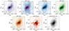 |
Fig. A.1. Resolution homogenised version of Fig.1, with the ALMA resolution as the target. The first row presents, from left to right, HST/ACS F814W (rest-frame 145 nm), JWST/NIRCam F115W (207 nm), F150W (270 nm), and F277W (499 nm). The second row shows JWST/F444W (800 nm), ALMA dust continuum emission around 156.9 μm, and ALMA [CII] 158 μm emission. The black contours are the (3+2k)σ levels (k ≥ 0) of the [CII] luminosity map, while the ellipses in the bottom left corners all panels indicate the synthesised ALMA beam. These images illustrate the filter coverage available across all galaxies in our sample. |
Appendix B: SED modelling parameters
Parameter values for different modules used for the CIGALE runs.
Appendix C: Assessing the validity of the SED modelling
We assess the impact of different parametrisations in the CIGALE SED modelling process on SFR estimates. To evaluate the reliability of each model configuration, we compare the SFR values derived by CIGALE (SFRSED) with those independently inferred from combined UV and far-infrared (FIR) measurements, following the methodology of Béthermin et al. (2023). Figure C.1 presents this comparison for VC875 as an example with each panel corresponding to a different set of CIGALE parameters. The one-to-one relation (dashed line) and the ±50% deviation lines (dotted) are included to facilitate a direct visual assessment of model performance.
It is important to emphasise that agreement between SED-based and UV+FIR SFR estimates does not necessarily guarantee the absence of systematic uncertainties or biases, since both methods may be subject to common assumptions regarding dust attenuation laws, SFHs, or IMFs.
 |
Fig. C.1. Comparison between SFR derived from SED modelling (SFRSED) and those measured from IR+UV observations (SFRIR + UV) for VC875, shown for different model parametrisations. From top to bottom: (first) the fiducial model using the Charlot & Fall (2000) dust attenuation law and a delayed SFH with a recent variation episode; (second) the same, but without the recent variation episode; (third) the fiducial model without ALMA dust luminosity constraints; (fourth) the Calzetti et al. (1994) attenuation law model. Blue points represent individual pixels, with error bars corresponding to the 16th and 84th percentiles of the SED-derived SFR distribution (see Sect. 3.1). Red arrows indicate upper limits. Black points show region-averaged SFR values computed using the B23 method. The dashed line indicates the one-to-one relation, and dotted lines mark the ±50% range. |
The top panel shows results from our fiducial model, which employs the Charlot & Fall (2000) dust attenuation law combined with a delayed SFH including a recent episode of star formation variation. This configuration achieves the closest agreement between SFR estimators, with most data points clustering near the one-to-one line.
When the recent SFH variation is excluded (second panel), the SED-based SFR estimates are systematically lower, with the majority of pixels lying above the one-to-one relation, showing a deterioration in fit quality.
Excluding the dust luminosity constraint from the modelling (third panel) results in systematic overestimation of SED-based SFRs relative to the UV+FIR values, with many points falling well beyond the −50% deviation line. In this situation, the error bars increase significantly, reflecting greater uncertainties in the fits. This highlights the critical role of including infrared constraints to properly model dust attenuation and derive reliable SFRs.
The fourth panel presents results obtained using the Calzetti et al. (1994) dust attenuation law. Across the sample, differences relative to the fiducial model are minimal. However, for CRISTAL_24 (see Fig. C.2), we observe the largest discrepancy between attenuation prescriptions: the Charlot & Fall (2000) law (top panel) achieves the best agreement between SFR estimators, with most data points lying close to the one-to-one line, while the fiducial model (centre panel) systematically underestimates SFRs and yields a lower fraction of well-fitted pixels. We verified that this difference is not attributable to the choice of the δ parameter in the Calzetti law, as letting δ vary produces identical results (bottom panel). Given the improved consistency for CRISTAL_24 and the more physically motivated nature of the Charlot & Fall (2000) law, we adopt it as our default attenuation model for the entire sample.
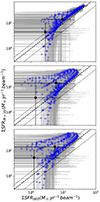 |
Fig. C.2. Same as Fig. C.1, but for CRISTAL_24. From top to bottom: Results using the Charlot & Fall (2000) dust attenuation model, results using the modified Calzetti et al. (1994) model with δ = 0, same but letting the δ parameter vary between -2.0 and 0.5 |
Appendix D: Validation of the likelihood model
To evaluate the accuracy and robustness of our fitting methodology, we perform an end-to-end simulation designed to replicate the observational conditions and intrinsic properties of our dataset. Specifically, we generate 1000 independent mock realisations. For each of them, we create first gas surface density maps composed of a random number of elliptical Gaussian clumps with varying amplitudes and positions. We then convolve this map with the ALMA beam. Using a fixed star formation relation characterised by a known slope, intercept, and intrinsic scatter, we derive the corresponding SFR surface density maps on a pixel-by-pixel basis. We then simulated the intrinsic scatter by multiplying this map by a map containing log-normal fluctuations at the scale of the ALMA beam with dispersion corresponding to the intrinsic scatter and a mean value of unity. This step is important, since we measure the intrinsic scatter at the scale of the ALMA beam, and applying a pixel-based scatter would lead to a smaller scatter after smoothing the maps by the beam.
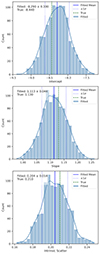 |
Fig. D.1. Distributions of the fitted parameters obtained from 1000 simulated datasets (see Appendix D). From top to bottom : intercept, slope, and intrinsic scatter. The blue histograms show the results from our likelihood-based fitting method, with the solid and dotted blue lines indicating the mean and the ±1σ intervals. The true input value used to generate the simulations is shown as a dashed green line. Each panel is annotated with the mean and standard deviation of the fitted parameter and the true input value in the top left corner. |
We then generate instrumental noise maps scaled to the noise properties of our ALMA data. We first convolve these noise maps to the same resolution, rescale their standard deviation, and added them to the gas maps. For the SFR maps, we applied the typical log-normal errors found by CIGALE for the real data. This process was repeated 13 times to produce a mock population comparable in size and complexity to our observed sample. Each mock dataset is subsequently analysed using our likelihood-based fitting procedure of Sect. 3.2, identical to what used for the real observations. We recover maximum likelihood solution of the slope, intercept, and intrinsic scatter parameters. The distributions of the fitted parameters across 1000 mock population realisations were then examined to assess the fidelity of the fitting method, see Fig. D.1.
We find that, for each parameter, the true input value lies well within the 1σ confidence interval of the recovered distribution. Still, small systematic offsets between the mean fitted values and the true parameters are observed. The intercept is overestimated by approximately 0.15 dex relative to the true value, while the slope and intrinsic scatter are underestimated by about 0.017 and 0.06 dex, respectively. These relative differences correspond to roughly 0.45, 0.39, and 0.43 times the respective 1σ uncertainties, indicating that the deviations are minor compared to the statistical errors. We note that the 1σ intervals from the mock ensemble are systematically smaller than those from the real data. It could be due to a better S/N or the larger number of beams with a [CII] signal in our simulation. We therefore conclude that our approach does not systematically bias the estimates of the key parameters of the star formation relation.
Appendix E: Alternative Fitting Methods
In addition to this primary analysis, we use two other fitting methods to assess the validity of the likelihood model and its maximisation approach: the Bayesian linear regression package linmix and the MCMC sampler emcee (Foreman-Mackey et al. 2013).
For the MCMC analysis, we configure 32 walkers with 1,000 steps per chain, discarding the first 100 steps as burn-in and thinning chains by a factor of 20 to mitigate autocorrelation. To take into account the correlation between pixels, we normalise the likelihood from Eq. 9 by the number of independent pixels per beam. This approach aims to approximate the number of independent points per resolution element. However, since beam smoothing may effectively yield twice as many statistically independent noise samples as naively expected (see Condon 1997; Condon et al. 1998), we thus divide the likelihood by twice the number of pixels per beam. The impact of this normalisation is illustrated by the following MCMC fitting results. Without any likelihood normalisation, we obtain  and
and  . When normalising the likelihood by twice the number of pixels per beam, the results broaden to
  and
and  . This demonstrates that accounting for the effective number of independent data points leads to larger and more realistic uncertainty estimates on the fitted parameters.
The linmix method uses Bayesian regression to account for measurement errors in both variables and intrinsic scatter, providing robust estimates of the slope, intercept, and intrinsic scatter of the studied [CII]-SFR relation. However, like in classical MCMC approach, it assumes uncorrelated pixels, ignoring spatial correlations within the beam and thus underestimate uncertainties in the presence of significant beam smoothing.
While both the linmix and MCMC fitting procedures provide estimates of the relation parameters and their uncertainties, they do not fully account for all sources of correlation, noise propagation, or population sampling effects present in our data. In particular, neither method can rigorously handle the spatial correlations and noise structure introduced by beam smoothing, nor the potential biases arising from the small sample size. For these reasons, we consider our primary resampling-based approaches described in Sect. 3.2 and Sect. 3.3 to provide more reliable and conservative estimates of the uncertainties and best-fit parameters for the [CII]–SFR relation.
Appendix F: Other sources property maps
As in Fig. 3, we show here example of spatially resolved physical parameters maps obtained with the CIGALE SED modelling for the other sources in the sample in Figs. F.1,F.2 and F.3. In each case, we have: stellar mass surface density (M⊙ kpc−1), SFR surface density averaged over 10 Myrs (M⊙ yr−1 kpc−2), mass-weighted age (Myr) and attenuation in FUV rest-frame (mag). Results are shown with the final selection used for the [CII]-SFR and KS relation analysis, that is pixels with S/N ≥ 2 in at least 3 photometric bands and where Σ[CII] > 5σ[CII]. Across the sample, we find that the peaks of stellar mass and SFR are generally aligned. In contrast, regions of highest SFR tend to coincide with diminished FUV attenuation, and the mass-weighted age maps reveal that the oldest stellar populations are preferentially located in regions of highest stellar mass surface density.
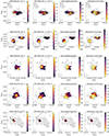 |
Fig. F.2. Similar to Fig. 3 for CRISTAL_06, CRISTAL_07, CRISTAL_09, CRISTAL_11 and CRISTAL_13 (top to bottom) |
All Tables
All Figures
|
Fig. 1. Multi-wavelength data for the galaxy VC875, shown at their native resolutions. From left to right: The first row presents HST/ACS F814W (rest-frame 145 nm), JWST/NIRCam F115W (207 nm), F150W (270 nm), and F277W (499 nm). The second row shows JWST/F444W (800 nm), ALMA dust continuum emission around 157 μm, and ALMA [CII] 158 μm emission. The contours are those of the ALMA [CII] line emission maps starting from 3σ increasing by steps of 2σ. Ellipses in the bottom left corners represent the central lobe of the PSF for HST and JWST images, and the synthesised beam for ALMA images. |
| In the text | |
|
Fig. 2. Native resolution image of VC875 (left panel) and the homogenised version matching the ALMA resolution (right panel) for the JWST/NIRCam F150W filter. The contours and ellipses are the same as in Fig. 1. |
| In the text | |
|
Fig. 3. Example of physical parameters maps obtained with the CIGALE SED modelling for VC875. From left to right: Stellar mass surface density (solar masses per square kiloparsec), SFR surface density averaged over 10 million years (solar masses per year per square kiloparsec), mass-weighted age (million years), and attenuation in the FUV rest frame (magnitudes). The contours are those of the [CII] luminosity map, starting at 3σ and increasing by steps of 2σ. The ellipse in the bottom left of each panel represent the synthesised ALMA beam. The maps are shown for the pixels having L[CII] ≥ 5σ[CII] and S/N ≥ 2 in at least three bands. |
| In the text | |
|
Fig. 4. Resolved [CII]-SFR relation for galaxies at z ∼ 5. The grey contours show the individual pixel distribution for the whole sample. Each pair of coloured points represents a high- and low-[CII] density average region for each galaxy of the sample following B23 methodology. The orange line and shaded region shows our best-fit power-law model from the tailored likelihood-based approach with the parameters in the top left corner (where log10(C0) is the value at g0 = 107.5 L⊙ kpc−2). The dashed black line presents the extrapolation of the relation derived from a spatially resolved sample of 46 nearby galaxies by Herrera-Camus et al. (2015). We represented the typical errors bars for the individual pixels across the sample with three black squares. |
| In the text | |
|
Fig. 5. Kennicutt-Schmidt relation using the α[CII] conversion factor (left) and the W[CII] version (right). The grey contours show the distribution of individual pixel measurements across the entire sample; the pair of points are the B23 region averages for individual galaxies, colour-coded by redshift. The dashed grey lines show constant gas depletion time. The dashed black line represents the Wang et al. (2022) KS relation for local Universe and high-redshift main-sequence galaxies. We show CO measurements of the global KS relation from the low-z COLD GASS sample (Saintonge et al. 2012, crosses) and at redshifts up to z ∼ 2.5 from the PHIBBS (Tacconi et al. 2013, plus signs) and PHIBBS2 (Freundlich et al. 2019, three-branch stars) programmes, together with a resolved z = 2.6 lensed starburst (Sharon et al. 2013, red points). |
| In the text | |
|
Fig. 6. Similar to Fig. 5. This time, symbols indicate integrated measurements for individual galaxies, colour-coded by interaction state: light blue for major mergers, light yellow for interacting systems, and orange for isolated galaxies, following the classification of Herrera-Camus et al. (2025). Symbol size encodes the total stellar mass and symbol shape denotes AGN identification: circles for non-AGNs, squares for AGN candidates, and triangles for robust AGNs as per Ren et al. (in prep.). The solid blue line shows the z = 4 relation from Kraljic et al. (2024), based on the 25% most massive galaxies in the NewHorizon simulation, while the solid red line indicates the NewCluster analogue (Han et al. 2025). Both relations are plotted over their effective gas mass ranges for direct comparison with our sample. |
| In the text | |
|
Fig. A.1. Resolution homogenised version of Fig.1, with the ALMA resolution as the target. The first row presents, from left to right, HST/ACS F814W (rest-frame 145 nm), JWST/NIRCam F115W (207 nm), F150W (270 nm), and F277W (499 nm). The second row shows JWST/F444W (800 nm), ALMA dust continuum emission around 156.9 μm, and ALMA [CII] 158 μm emission. The black contours are the (3+2k)σ levels (k ≥ 0) of the [CII] luminosity map, while the ellipses in the bottom left corners all panels indicate the synthesised ALMA beam. These images illustrate the filter coverage available across all galaxies in our sample. |
| In the text | |
|
Fig. C.1. Comparison between SFR derived from SED modelling (SFRSED) and those measured from IR+UV observations (SFRIR + UV) for VC875, shown for different model parametrisations. From top to bottom: (first) the fiducial model using the Charlot & Fall (2000) dust attenuation law and a delayed SFH with a recent variation episode; (second) the same, but without the recent variation episode; (third) the fiducial model without ALMA dust luminosity constraints; (fourth) the Calzetti et al. (1994) attenuation law model. Blue points represent individual pixels, with error bars corresponding to the 16th and 84th percentiles of the SED-derived SFR distribution (see Sect. 3.1). Red arrows indicate upper limits. Black points show region-averaged SFR values computed using the B23 method. The dashed line indicates the one-to-one relation, and dotted lines mark the ±50% range. |
| In the text | |
|
Fig. C.2. Same as Fig. C.1, but for CRISTAL_24. From top to bottom: Results using the Charlot & Fall (2000) dust attenuation model, results using the modified Calzetti et al. (1994) model with δ = 0, same but letting the δ parameter vary between -2.0 and 0.5 |
| In the text | |
|
Fig. D.1. Distributions of the fitted parameters obtained from 1000 simulated datasets (see Appendix D). From top to bottom : intercept, slope, and intrinsic scatter. The blue histograms show the results from our likelihood-based fitting method, with the solid and dotted blue lines indicating the mean and the ±1σ intervals. The true input value used to generate the simulations is shown as a dashed green line. Each panel is annotated with the mean and standard deviation of the fitted parameter and the true input value in the top left corner. |
| In the text | |
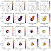 |
Fig. F.1. Similar to Fig. 3 for CRISTAL_01, CRISTAL_02, CRISTAL_03, and CRISTAL_04 (top to bottom) |
| In the text | |
|
Fig. F.2. Similar to Fig. 3 for CRISTAL_06, CRISTAL_07, CRISTAL_09, CRISTAL_11 and CRISTAL_13 (top to bottom) |
| In the text | |
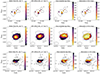 |
Fig. F.3. Similar to Fig. 3 for CRISTAL_15, CRISTAL_19, and CRISTAL_24 (top to bottom) |
| In the text | |
Current usage metrics show cumulative count of Article Views (full-text article views including HTML views, PDF and ePub downloads, according to the available data) and Abstracts Views on Vision4Press platform.
Data correspond to usage on the plateform after 2015. The current usage metrics is available 48-96 hours after online publication and is updated daily on week days.
Initial download of the metrics may take a while.