| Issue |
A&A
Volume 702, October 2025
|
|
|---|---|---|
| Article Number | A78 | |
| Number of page(s) | 17 | |
| Section | Interstellar and circumstellar matter | |
| DOI | https://doi.org/10.1051/0004-6361/202556172 | |
| Published online | 07 October 2025 | |
Multiwavelength analysis of polarized light in HD 100453★
1
Univ. Grenoble Alpes, CNRS, IPAG,
38000
Grenoble,
France
2
Institute for Particle Physics and Astrophysics, ETH Zurich,
Wolfgang Pauli Strasse 17,
8093
Zurich,
Switzerland
3
Department of Earth Science and Astronomy, The University of Tokyo,
Tokyo
153-8902,
Japan
4
Astronomy Department, University of California Berkeley,
Berkeley,
CA
94720-3411,
USA
5
Anton Pannekoek Institute for Astronomy, University of Amsterdam,
Science Park 904,
1098XH
Amsterdam,
The Netherlands
6
School of Natural Sciences, Center for Astronomy, University of Galway,
Galway
H91 CF50,
Ireland
★★ Corresponding author: This email address is being protected from spambots. You need JavaScript enabled to view it.
Received:
30
June
2025
Accepted:
12
August
2025
Abstract
Context. HD 100453 disk is a prototypical companion-disk interaction system hosting a pair of spirals and a substellar companion.
Aims. We present new noncoronagraphic high-contrast imaging observations of HD 100453 with V filter on SPHERE/ZIMPOL. We aim to accurately measure the reflected polarized intensity, the disk intensity, and the degree of polarization at multiwavelength; characterize the dust properties in the disk ring and the companion-driven spiral arms; and search for the radial dependencies of dust scattering properties within the disk.
Methods. We combined high-contrast imaging data of the reflected light from 0.55 to 2.2 μm using the V, I′, J, and Ks band data of ZIMPOL and IRDIS at VLT/SPHERE. For each observational epoch, we corrected for the smearing effect to derive the intrinsic disk-integrated polarized flux. We applied reference differential imaging to extract the disk intensity for the V and Ks bands using star hopping observations. We then used RADMC-3D radiative transfer modeling with a parametrized Henyey–Greenstein phase function to constrain the dust properties.
Results. For the integrated intrinsic polarized flux of the disk, we derived a steady increase with wavelengths from Qφ/I★(V) = 0.3% to Qφ/I★(K) = 1.2%. We obtained the first V-band total intensity for HD 100453 with ZIMPOL star hopping. The integrated total flux Idisk/I★(V) = 1.5% increases to Idisk/I★(K) = 4.8%. Both the total intensity and the polarization fraction show red colors, and the intrinsic maximum degree of polarization increases moderately from 40% to 55%. From the V to Ks band, the dominating dust in the outer disk has an increasing scattering albedo and degree of polarization, while the asymmetry parameter slightly decreases. The outer disk of HD 100453 contains sub-micron-sized low porosity grains/aggregates. The cavity in scattered light is not empty and is replenished with optically thin dust with a maximum size of ≤ 0.1 μm. The linear polarization is higher in the spiral region than in the other regions, suggesting different dust properties in those regions.
Key words: polarization / radiative transfer / scattering / protoplanetary disks / stars: pre-main sequence
Based on observations collected at the European Southern Observatory under ESO programs 110.245U.001 and 105.20JB.001.
© The Authors 2025
 Open Access article, published by EDP Sciences, under the terms of the Creative Commons Attribution License (https://creativecommons.org/licenses/by/4.0), which permits unrestricted use, distribution, and reproduction in any medium, provided the original work is properly cited.
This article is published in open access under the Subscribe to Open model. This email address is being protected from spambots. You need JavaScript enabled to view it. to support open access publication.
1 Introduction
With the development of high-contrast and high-resolution direct imaging, a variety of structured protoplanetary disks have been revealed (Benisty et al. 2023). Multiwavelength polarimetric differential imaging (PDI) offers a unique perspective from which to characterize the dust scattering properties. Among the polarization observables, the degree of polarization of the scattered light is particularly valuable because it is less sensitive to the overall disk structure, thus allowing for more accurate diagnostics of dust properties, such as grain size and porosity (Min et al. 2016; Tazaki & Dominik 2022), which directly influences planet formation processes (Garcia & Gonzalez 2020). Studying dust evolution is critical because grain growth depends on local disk conditions, such as turbulence, temperature, and interactions with companions and embedded planets (Birnstiel 2024).
HD 100453 is an ideal system to investigate to gain insight into environment-dependent dust evolution. HD 100453A is a Herbig A9Ve star in the lower Centaurus Association, located at 103.8 pc (Gaia Collaboration 2023), with a close M-type companion, HD 100453B, separated by 1.05″ (Collins et al. 2009). The main star shows an IR-excess typical for a transition disk with strong emission from hot dust around 2–5 μm another maximum around 25 μm from cold dust, and polycyclic aromatic hydrocarbons emission bands (Malfait et al. 1998; Meeus et al. 2001). The cold dust component is well resolved in scattered light, showing a disk with a cavity of r = 0.14″, a bright rim inclined by 38°, two symmetric trailing spiral arms, and two shadows on opposite sides of the disk ring in the NE and SW (Wagner et al. 2015; Benisty et al. 2017). The two shadows are caused by a misaligned inner disk, which accounts for the hot dust emission in the near-IR. Atacama Large Millimeter/submillimeter Array (ALMA) Band 6 revealed CO isotopolog emissions, showing gas presence within the disk cavity (van der Plas et al. 2019) and proved that the disk is gas poor (van der Plas et al. 2019; Collins et al. 2009). The subsequent Band 7 reached a higher angular resolution and detected spirals in both CO and dust emission, with the southern spiral connecting to the companion (Rosotti et al. 2020). These features make HD 100453 a well-observed and studied system across a wide range of wavelengths.
The origins of the spirals and shadows in HD 100453 have been widely investigated. Popular explanations include the massive companion, the optically thick misaligned inner disk, and undetected planets. Previous works have characterized the system’s spiral morphology and companion properties (Benisty et al. 2017; Wagner et al. 2018; Gonzalez et al. 2020), yet a detailed analysis of dust properties in the disk, particularly across its substructures comparing the ring, spirals, and cavity, is lacking. Understanding the dust characteristics is critical, as different dynamical environments within the disk can significantly alter the grain size distribution through processes such as dust filtration (Zhu et al. 2012; Pinilla et al. 2016) and spiral-induced dust concentration (Dipierro et al. 2015; Cuello et al. 2019). We aim to use multiwavelength polarimetric observations to reveal variations in dust grains across different disk regions, providing insight into how disk-companion interaction influences dust growth.
In this paper, we present multiwavelength polarimetric imaging, including the first V-band observation and new observational data at the I′, J, and Ks bands for HD 100453, and combine them with the archival Ks band in order to investigate the dust properties and explore the variability seen in scattered light. In Section 2 we describe the selected observations and the data reduction procedure. In Section 3, we measure the disk-integrated polarized flux, the disk intensity, and the fractional polarization considering the point spread function (PSF) smearing effect. In Section 4, we use the radiative transfer (RT) RADMC-3D disk model to constrain the dust scattering properties in different regions. In Section 5, we discuss dust size, structure, and composition in the disk and relate them to the forming environment. We summarize the main results in Section 6.
VLT/SPHERE Polarimetrie imaging data and corresponding observing conditions.
2 Observations and data reduction
2.1 Selected observations
New HD 100453 data were taken in 2023 (ESO Program ID: 110.245U.001, PI: J. Ma) using the SPHERE/VLT high contrast adaptive optics instrument (Beuzit et al. 2019). This observation is specifically designed for accurate multiwavelength, photo-polarimetric measurements of the scattered light from the disk to characterize dust properties. The data include nonsaturated, short integrations in the V, I′, J, and Ks-bands, and longer integrations with saturation at V using a star-hopping procedure to calibrate the PSF with reference star observations. All the observations are taken in P1 mode with field rotation to correct for fixed instrument features, reach a higher precision for polarimetry, and facilitate angular differential imaging for the disk intensity extraction.
Nonsaturated observations were carried out for all four wave-lengths, using fast read-out mode and short exposure time for the V and I′-band observations with ZIMPOL, and neutral density (ND) filters for the J and Ks-bands observations with IRDIS. Such nonsaturated observations provide simultaneous measurements of the polarized intensity of the disk and the flux in the PSF peak of the central star to monitor and account for temporal variation of the PSF convolution in the data (Tschudi & Schmid 2021).
The star-hopping sequence at V (labeled V-hop) is designed to switch between long-exposures and short-exposures on target, combined with hopping to the PSF reference star for long-exposures. We designed three iterations of hopping, each containing three polarimetric cycles of long exposures and one polarimetric cycle of short exposures on HD 100453, and one polarimetric cycle of long exposure on reference star. The long exposures on science target and reference stars are saturated in the center, but deep enough to allow disk intensity extraction. Short exposures in between monitor the stellar (and disk) variability and the seeing condition. Details of the observing conditions and PSF quality parameters are summarized in Table 1. Analyzing reflected light from compact disks regions, as in this case, is very difficult with high precision polarimetry, as even small PSF variations can significantly affect the measured polarization signal (Tschudi & Schmid 2021). Therefore, each epoch of observation is designed to have (quasi-) simultaneous unsaturated PSFs so that fast PSF variations can be taken accurately into account.
This study also includes archival SPHERE Ks-band data of HD 100453 taken in June 2022 from a coronagraphic Ks-band survey program on protoplanetary disks using star hopping (Program ID: 105.20JB.001, PI: M. Benisty). The hopping sequence for HD 100453 lasted for more than two hours, starting and ending with the science target, and hopping to a reference star for six times. For each hop on the science target, two or three long polarimetric cycles were taken with coronagraph N_ALC_Ks. The observation does not include short exposures in between, only two flux frames were taken with ND filter, but without polarimetric optical components, one before and one after all the polarimetric cycles. The observational results of this program are published in Ren et al. (2023).
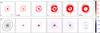 |
Fig. 1 Polarized intensity images Qφ(x,y) and Uφ(x,y) for V, I′, J, and Ks band. All images are normalized to the integrated stellar intensity I★ and their pixel scale (3.6 × 3.6 mas2 for ZIMPOL and 12.25 × 12.25 mas2 for IRDIS). The shared color bar is indicated on the right. All the images are cut to 1.0 × 1.0″ and the black bar in Qφ(V) indicates 0.2″. The dashed lines in Uφ(V) enclose the integration region for the cavity, the rim, and the spiral respectively. The semitransparent circle in K-hop represents the inner working angle (IWA) = 0.125″ limited by the coronagraph. North is up and east to the left. |
2.2 Data reduction
ZIMPOL data were reduced with the IDL pipeline sz-software as described in Schmid et al. (2018), and the IRDIS data were reduced with IRDAP (IRDIS Data reduction for Accurate Polarimetry) pipeline (van Holstein et al. 2020). For each raw data frame, these dedicated pipelines perform basic image extraction, bad pixel correction, dark subtraction, flat-fielding, and centering steps. The sz-software allow for an extra beamshift correction, which is required for high-performance Polarimetrie data. The pipelines perform standard double-difference to derive the Stokes parameters Q = I0 – I90, U = I45 – I135, and double-addition methods to compute total intensities IQ = I0 + I90, IU = I45 + I135. We define the final total intensity as the average I = (IQ + IU)/2.
On top of the data reduction with their dedicated pipelines, we apply an extra step to subtract the stellar polarization. For all integrations without saturation, we measure the fractional polarization  and position angle θ = 1/2 · arctan (U/Q) in a r = 0.05″ round aperture that encloses the stellar PSF core. For long-integrations in V-band when the center is saturated, the stellar polarization is measured in an annulus covering the radius range [0.29, 0.36]″ of the speckle ring at about 20λ/D which is mostly caused by light from the central source, but also contains small contributions from the polarization signal from the disk.
For Ks-band long-integration, the stellar polarization is measured between [0.98, 1.49]″ in the speckle ring at this wave-length, which is located outside the disk emission, and the SE quadrant is excluded from the integration region to avoid contamination from the companion. We note that the unresolved central source contains the signal from the inner disk.
We measured for HD 100453A a very low degree of polarization p < 0.2% at V, I, and J, indicating that contributions from intrinsic stellar polarization, instrumental polarization, and interstellar polarization are small. A low residual instrumental polarization is typical for SPHERE polarimetry, and also a low interstellar polarization is expected for HD 100453 because of its low interstellar extinction (Malfait et al. 1998). The Ks-band shows a higher polarization p = 0.6% with a position angle of about θ ≈ 170°. This is compatible with an intrinsic polarization perpendicular to the orientation of the major axis of the unresolved hot disk of 80° according to the model of Benisty et al. (2017), which dominates the central source emission in the Ks-band. Unfortunately, the uncertainties in this interesting polarization result are not well defined and would require much improved instrument calibration procedures to correct residual instrumental effects and achieve reliable values at the Δp < ±0.1% level. Therefore, we subtracted the measured stellar polarization (p, θ) at each wavelength from the Stokes Q and U maps using Q(x,y) = Qobs (x, y) – I(x, y)p cos θ and U(x, y) = Uobs(x, y) – I(x, y)p sin θ so that the central star has zero polarization (Schmid & Ma 2025).
For Ks-band observations, we carried out an extra back-ground subtraction step on the intensity frames, which is necessary for later quantitative analysis. And for K-hop observation, we applied a transmission correction for the coronagraph N_ALC_Ks, which is indispensable for compact disks such as HD 100453 whose inner edge is close to the inner working angle(IWA) = 0.125″ of the coronagraph. These steps are detailed in Appendices A.1 and A.2.
As the last step, we calculated the azimuthal polarization parameters Qφ(x, y) and Uφ(x, y) maps from the reduced Stokes polarization Q(x, y) and U(x, y) maps:
 (1)
(1)
 (2)
(2)
where φ is the position angle of the map location (x, y) to the central star from north over east. Fig. 1 presents the mean Qφ(x, y) and Uφ(x, y) maps for the different data sets.
3 Data analysis
3.1 Stellar intensity
HD 100453A is classified as a Herbig Ae/Be star, which are young pre-main-sequence stars known for variability. Photometric results from the Hipparcos satellite have shown variations with a scatter in the star brightness of ±0.026 mag during about 3.5 years. We neglect such variations for our photo-polarimetric study, which is mostly based on relative measurements between polarized flux signals and the intensity of the system HD 100453A.
We used the total intensity of the main star HD 100453A as the reference value I★, including the contributions from the circumstellar disk but with the companion filtered out. For this we first calculated the azimuthally averaged radial profile I★(r) and its standard deviation ΔI★(r) in the annulus section, defined by r = [0.6″, 1.6″] and φ = [0, 90°] ⋃[180°, 360°] excluding the quadrant regions with the companion. We then replace in the quadrant of the companion φ = [90°, 180°] all points I(r, φ) with intensities outside the range I★(r) + ΔI★(r), typically with a higher value because of the additional contribution from the companion, by a random number drawn from a Gaussian distribution with mean I★(r) and standard deviation ΔI★(r).
The intensity I★ for HD 100453A is then integrated within the round aperture of 3″-diameter for all nonsaturated images. The uncertainty for I★ is the standard deviation for all intensity frames for a given instrument setting. For K-hop, only two flux frames are available and we use half of the difference between the two as uncertainty for I★. The resulting uncertainty is 2%, consistent with deviations obtained for other settings.
We used the companion-subtracted images for HD 100453A as a proxy for the PSF profiles of individual observations, which are used to correct PSF smearing effects. The contribution of the extended disk intensity to the I★ value is between 1% and 4%, as is derived later. Temporal variations in atmospheric turbulence change the shape of the PSF profile, much more than the flux contribution of the disk. Therefore, using the measured intensity distribution for HD 100453 as PSF for the convolution correction will have only a small effect on the derivation of the intrinsic polarization signal.
In addition, the difference between the total intensity frame and the filtered intensity frame gives the intensity of the companion. We derive the flux ratio between the Β and A components about 0.05% at V and 1.25% at Ks. More details for all used filters and magnitudes are given in Appendix A.3.
Observed polarized flux Qφ/Ι★ integrated in different apertures for HD 100453 for each observing date.
3.2 Polarized disk intensity
The measurement of the azimuthal polarization Qφ of the circumstellar scattering regions depends on the spatial resolution of the observations. The main effect of PSF smearing in polarimetry is the cancellation between positive and negative signals in the Stokes Q and U quadrants caused by scattering. Therefore, one needs to take the PSF convolution into account to derive the intrinsic photo-polarimetric signal. All short exposures obtained in 2023 provide the polarization signal and the unsaturated intensity signal simultaneously. This allowed us to correct for the variable PSF smearing effects cycle by cycle following the procedure described in Ma et al. (2024).
The correction relies on the fact that convolution is a linear operation. The PSF smearing of an inclined disk can be simulated by summing the convolutions of narrow concentric ellipses that align with the inclined geometry. For a given PSF, the smearing is stronger at small radii and weaker at larger radii. Using this principle, we derive a two-dimensional correction map for each Polarimetrie cycle to correct the observed disk images. Simulations in Ma et al. (2024) show that this approach recovers the PSF-smearing-corrected intrinsic polarization signal  with an error of less than a few percent for disks with roughly an ellipse-like appearance such as HD 100453.
For our analysis, we derive the intrinsic azimuthal polarization  within the elliptical aperture, with radius range of [0.10, 0.86]″ inclined by 38°, as shown in Fig. B.1 for each Polarimetrie cycle of all instrument settings. The results are listed in Table 2 and plotted in Fig. 2.
For the V, I, J, Κ observations and V-hop short integrations with simultaneous Qφ and I★ measurements, we report the mean  value and standard deviation of all cycles. For the K-hop data where I★ and Qφ were obtained separately, error propagation is applied to derive the final Qφ/I★ and
  values. We note that for K-hop, the central 125 mas region is masked out, so the resulting values represent lower-limit estimates. The V-hop long-integrations lack simultaneous unsaturated PSF information and the seeing conditions varied over the two-hour observation. This explains the large standard deviation ΔQφ/Qφ = 16%. Fortunately, nonsaturated short integrations taken in between the long integrations helped to account for the seeing variations, though the relative uncertainties remain larger than those in the other datasets. Fig. 2 includes the measurement in the R′, I′, and J-bands from Ma et al. (2024) using the same integration aperture. The excellent agreement between the different measurements indicates that the azimuthal polarization signal of HD 100453 is stable.
We also measured the integrated flux from disk substructures using concentric elliptical apertures: the cavity, the rim, and the spirals, corresponding to the radial ranges of [0.10, 0.13]″, [0.13, 0.24]″, and [0.24, 0.40]″ respectively for epochs that have simultaneous PSFs. Flux correction was applied to observed polarization for the rim and spirals regions, and the resulting intrinsic values  and
and  are summarized in Table 2. The
  shows a faster increase with wavelength than the
  , hinting at different dust species in the substructures, which we discuss in Section 5.2. We list only the observed integrated polarized flux from the cavity
  in Table 2 because the innermost region is too faint and too close to the star for a reliable PSF-smearing correction using the method in Ma et al. (2024). Instead, we correct the cavity flux using the forward-modeling approach described in Section 4.3. We note that the substructure apertures do not fully cover the total flux integration region, which was chosen conservatively to include all smeared signal, so their sum does not equal the total flux.

3.3 Disk intensity
The V-hop and K-hop observing sequences used a star-hopping strategy (Wahhaj et al. 2021), taking quasi-simultaneous total intensity observations of a PSF reference star enabling reference differential imaging to extract the disk intensity map for HD 100453 A. The reference star is chosen to have a similar spectral type and magnitude as the science target but hosts no disk. For the first time, this study applies this method to observations with the SPHERE/ZIMPOL camera. For V-hop, we obtained 54 total intensity images on target Itar(x, y) and 18 images of total intensity images on reference star Iref (x, y). For K-hop, we treated IQ and IU separately to match the number of image with V-band, resulting in 46 target images and 12 reference images in total.
The disk signal can be extracted from the difference
 (3)
(3)
where a is a constant scaling factor optimized to minimize the residuals within the defined fitting region with preferentially no contributions from the disk for each reference image. The residual is defined as the sum of the relative squared differences in each pixel over the fitting region Σ:
 (4)
(4)
where the fit image, Ifit, is defined as
 (5)
(5)
Ideally, the fitting region, Σ, should exclude any disk signal. The speckle ring is usually a good choice for this fitting region because it contains a strong stellar signal while minimizing the contributions from the disk. However, the PSF in the V-band introduces a nonnegligible extended disk halo component, Ihalo, that spreads the disk signal into the surrounding area (Fig. 6). This smeared component must be considered to avoid oversub-traction of disk intensity for the V-band. A quantitative analysis of this effect is provided in Appendix B, where we demonstrate that even a small contamination from the halo in the fitting region can cause significant errors when the disk is faint compared to the stellar PSF. Therefore, for V-band, we modified the fitting function to include the halo component:
 (6)
(6)
The fitting regions are shown in Fig. B.1. For V-hop, we adopted an annulus between [0.43, 0.76]″, chosen to include sufficient stellar signal while avoiding bright spirals. The halo component Ihalo(x, y) = Ihalo(r) is assumed to be radially symmetric, and is fitted using the disk model Setup A (introduced in Section 4), which follows exponential fall-off with radius.
For K-hop, we estimated that the halo component of the disk intensity is negligible, and we set Ihalo = 0 in the fitting process. The fitting region is defined as an annulus between [0.98, 2.14]″, with two circular apertures excluded to mask the companion and the known background star in the NE direction (Collins et al. 2009; Wagner et al. 2015).
For a given target image Itar, we search for the best-fitting scaling value a for each reference intensity image Iref and evaluate the result using the residual. We average the three best-fitting results among all scaled-Iref and obtain Ibest(x, y)-image for this given target image Itar. We apply this process for each target image and obtain 54 and 46 Ibest(x, y)-image for V and Ks-band, respectively. Among all Ibest images at given wavelength, we select the 10 with the lowest residuals (representing the top 20% in PSF subtraction quality) and compute their average to produce the final disk intensity map Idisk(x, y), shown in Fig. 3. The standard deviation among the selected images is used as a conservative uncertainty estimate, which is primarily driven by the seeing variability.
The extracted total disk intensity resembles the structure seen in polarized intensity. At V-band, the disk signal partly coincides with the strong speckle ring from the PSF near 0.4″, and therefore, the extracted intensity signal is noisy. The Ks-band disk intensity is less affected by speckle noise. In both bands, the companion and the background star are recovered.
For the integrated intensity, we used the same elliptical integration region as for the polarized intensity. We integrated the disk total intensity in the best 10 Idisk(x, y) images, with the mean and standard deviation taken as the final flux and uncertainty. The measured disk intensity values are Idisk/I★ = 1.2 ± 0.3% for V-hop and 3.8 ± 0.5% for K-hop. We note that for K-hop data, we adopt IWA=0.125″, so the integrated flux Idisk represents a lower limit. Moreover, the Idisk values are not yet corrected for the PSF convolution, which redistributes substantial disk intensity signal to regions outside the measuring aperture. This effect is quantified with convolved disk models in Section 4 to derive intrinsic disk parameters.
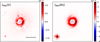 |
Fig. 3 Extracted disk intensity map Idisk(x, y) for the V- and Ks-bands, cut to 2.0 × 2.0″. The black bar indicates 0.5″. The central 0.1″ and 0.125″ are masked out as the IWA for V and Ks respectively. |
3.4 Degree of polarization
From the observed polarized intensity and total intensity maps for the disk, we derive the degree of polarization map as pdisk(x, y) = Qφ(x, y)/Idisk(x, y). For each of the 10 best-fitting maps Idisk(x, y), we use the corresponding cycle of Qφ(x, y) to calculate pdisk(x, y). The final result is the mean of these 10 maps, shown in Fig. 4, zoomed into 1 × 1″. To highlight the substructures, different color scales are applied for two bands. The standard deviation among the 10 images is taken as the uncertainty σ(pdisk). Pixels with low disk signal and high uncertainties exceeding 100% (for V-band) and 50% (for Ks-band) of the mean value are not shown. These maps present the convolution-smoothed spatial distribution of pdisk. While the regions with strong disk signals are less affected by systematic errors, the uncertainties per pixel remain large with deviations ±Δpdisk/pdisk of 40% for V-band and 20% for Ks-band.
The key observable derived from the pdisk maps is the maximum degree of polarization max(pdisk). For a disk with a given surface structure, this max(pdisk) typically occurs where the scattering angle is close to 90°, producing a high degree of polarization (Ma & Schmid 2022). Such favorable scattering angles naturally arise in most disk geometries, making max(pdisk) a robust and widely applicable diagnostic for characterizing dust scattering properties across different wavelengths and disk types (Tazaki & Dominik 2022).
For the determination of max(pdisk), we select the top 10% of pixels with uncertainties ±Δpdisk/pdisk below 20% of the mean value. The selected pixels are concentrated on the SE side of the major axis at V-band, and distributed on the major axis and the spiral tail at Ks-band. The final max(pdisk) values are taken as the average over these pixels, with the uncertainty dominated by the pixel-wise variation. The measured max(pdisk) are 28 ± 2% and 39 ± 4% respectively.
We note that the pdisk represents observed values, as both Qφ(x, y) and Idisk(x, y) are smeared by PSF convolution. Despite this limitation, several interesting features are already visible in the observed pdisk maps. In the pdisk(V) map, the SE side shows a higher degree of polarization (28%) compared to the NW side (21%). The origin of this asymmetry remains unclear. In the pdisk(K) map, the NE spiral exhibits an enhanced degree of polarization. In both pdisk(V) and pdisk(K) maps, the shadowed region exhibits a slightly lower degree of polarization, leading to discontinuities in the azimuthal variance along the rim. It is also important to note that, although the coronagraph leads to signal loss in both polarized intensity and total intensity, the pdisk is not affected at all as long as the transmission function is rotationally symmetric, because the same transmission correction map applies to Qφ and Idisk.
We also measured the disk-averaged degree of polarization 〈pdisk〉 = 16 ± 5% at V-band and 33 ± 6% at Ks-band. These values are derived directly from the observed polarization and intensity  in the given elliptical aperture and does not consider that the PSF convolution effects are different for the Qφ and Idisk signal (Schmid & Ma 2025). This problem is taken correctly into account with the forward modeling results from Sect. 4 providing intrinsic disk values.
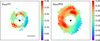 |
Fig. 4 Observed degree of polarization pdisk(x, y) for V- and Ks-bands cut to 1.0 × 1.0″. The black bar in the V-band subfigure indicates 0.2″. The star marker indicates the position of the central host star. |
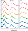 |
Fig. 5 Radial profiles of polarized intensity Qφ(r) along both sides of the major axis (left), near side (middle), and far side (right). All profiles have been normalized to the peak value along the major axis and shifted by one for clarity. The standard deviation among all cycles at a given epoch is indicated as the error bar. The shaded region indicates the cavity region [0.10, 0.13]″. |
3.5 Radial profile and brightness ratio
To characterize the scattering behavior of dust grains in the disk in more detail, we calculate the radial profiles within 30° wedges centered at position angle = 142° and 322° (major axis), 232° (near side), and 52° (far side). The mean profiles for each instrument setting are plotted in Fig. 5. V and Ks bands have two epochs of observations. The error bars represent the standard deviations between the profiles for all cycles of a given instrument setting. All profiles are normalized to the peak value along its major axis.
To quantify the observed asymmetries, we define brightness ratios based on these profiles (Table 3). The near-to-far side ratio RN/F is defined as the peak brightness on the near side divided by that on the far side. The near-to-major axis ratio RN/M is the peak brightness on the near side divided by that along the major axis. In addition, to examine the relative brightness of the two spiral arms, we define Rsp as the ratio of the mean value in the radial range [0.18, 0.20]″ of the near side profile, divided by the mean value in the radial range [0.22, 0.24]″ on the far side profile. Each ratio is computed for both polarized intensity and the total intensity, and we use superscripts to indicate the radiation component, RPI for polarized intensity and RI for total intensity.
These brightness ratios are sensitive to the dust scattering phase function and depend on the single scattering albedo and asymmetry parameters given the disk geometry (Ma & Schmid 2022). We find that RI is higher than RPI in all measured ratios, due to stronger forward scattering in total intensity. Both  and
and  decrease with wavelength, suggesting that the scattering becomes less anisotropic at longer wavelengths. This aligns with scattering grain sizes comparable to the observing wavelength. In contrast, the spiral brightness ratio
  remains approximately constant with wavelength, hinting at a different grain population or scattering regime in the spiral arms compared to the ring. These quantities and trends serve as diagnostic constraints in our later dust-scattering properties analysis.
All V-band profiles show for the innermost part near r ≈ 100 mas, inside the disk cavity, a substantial polarization signal. The contribution is much weaker for the I′-band, and hardly visible in near-IR. This indicates the presence of dust scattering inside the cavity, which is particularly strong at short wavelengths, and shows a bluer color than the dust in the rim. Notably, this polarized signal has not been detected before and is only revealed thanks to the high spatial resolution and short-wavelength coverage of the V-band observations.
Brightness ratios for all epochs.
4 Model
Due to the complex substructure in HD 100453, various disk models have been developed, especially to study the disk-companion interaction (Wagner et al. 2018; Gonzalez et al. 2020; Nealon et al. 2020). While these hydrodynamic models reproduce ALMA dust emission and gas kinematics, they are not suited for a quantitative comparison with the observed polarized intensity and total intensity to characterize the dust scattering properties.
To interpret the observed wavelength-dependent polarized intensity, total intensity, and degree of polarization, we adopt the parametric disk model from Benisty et al. (2017), originally built with MCMax (Min et al. 2009). This model also successfully reproduces the system’s SED, especially the outer disk’s infrared excess, providing a physically consistent dust density structure. We fully adopted the stellar, inner and outer disk parameters, and rebuilt the 3D dust structure with RADMC-3D (Dullemond et al. 2012) without dust settling. This simplification is justified as the micron-sized and smaller grains responsible for scattered light are expected to be well coupled to the gas and remain suspended in the disk surface layers. The NE and SW spiral arms param-eterizations are slightly adjusted to better match the observed morphology (summarized in Table C.1). Radiative transfer simulations are then performed in full scattering mode, launching 106 photon packets to produce polarized and total intensity images for the central wavelength of each filter. Although this model does not follow a self-consistent hydrodynamical evolution, and the spirals are implemented via artificial scale height enhancements, it offers the flexibility to match observed features in scattered light and allowed us to directly vary dust scattering properties.
In this section, we start from the model as presented in Benisty et al. (2017) and explore modified setups informed by our observed constraints, aiming to characterize the dust properties in the disk. An overview of the simulated images for each setup is presented in Fig. 6, and we discuss them individually in the following subsections.
4.1 Setup A: DIANA standard dust
This is a reproduction of Benisty et al. (2017) with minor adjustments to the geometric parameters of the spirals. The model assumes single dust species, the DIANA standard dust model, with the composition adopted from Woitke et al. (2016), and a power-law size distribution n(a) ∝ a−3.5 between amin = 0.01 μm and amax = 1 μm following Benisty et al. (2017). The refractive index is calculated assuming the Bruggeman mixing rule. The opacity and the scattering matrix are calculated with a distribution of hollow spheres (DHS, Min et al. 2005) approximation assuming 25% porosity.
This model was shown to reproduce the Qφ (x, y) observation at I′-band in Benisty et al. (2017), and it roughly matches the V-band observation (Figure 6 second row), as expected for a not too different wavelength. However, it fails to reproduce the Ks-band observations. Both the simulated polarized intensity Qφ and total intensity Idisk are significantly underestimated. Moreover, the simulated Qφ(x, y) lacks the near side, while the simulated Idisk(x, y) shows a too bright near side and too faint far side relative to the observation at Ks-band. The underpredicted brightness is due to the assumed dust’s low albedo and strong forward scattering. The strong forward scattering also produces the too bright near side in simulated Idisk(x, y), while the deficit of polarization in low scattering angles causes the missing front side in the simulated Qφ(x, y).
These discrepancies indicate that the DIANA standard dust is unlikely to dominate the surface layer of the disk. We tested variations in the maximum grain size, including both smaller and larger values up to several microns, but none produced satisfactory matches to the observations. To better constrain the dust properties without exhaustively exploring different compositions, size distributions, or porosities, we opt to characterize the dust via its scattering behavior. In the following setups, we define the scattering phase function using the Henyey–Greenstein formalism (Henyey & Greenstein 1941), which allows for more direct control over the key scattering parameters.
4.2 Setup B: Henyey–Greenstein dust approximation
We introduce a user-defined dust species “HG dust”, for which the scattering matrix is fully described by three parameters: the single scattering albedo ω, the asymmetry parameter ɡ, and the maximum degree of polarization pmax. The Mueller matrix elements are defined as
 (7)
(7)
 (8)
(8)
 (9)
(9)
where μ = cos θscat. The Kscat is adopted from the DIANA standard model to preserve realistic scattering opacities. Here, F11 represents the scattering phase function, which is the scattered intensity as a function of scattering angle. The element –F12 is often referred to as the polarized scattering phase function. And –F12/F11 gives the degree of linear polarization, which is a symmetric bell-shaped profile centered at the scattering angle 90°, with its amplitude scaled by pmax. We assume symmetric F21 = F12, F11 = F22 and F33 = F44 which holds for spherical particles and for a collection of randomly oriented nonspherical ones. We neglect the circular polarization by setting all the other elements to 0. While ω does not appear explicitly in the scattering matrix element, it defines the absorption opacity κabs via ω = κsca/(κsca + Kabs), required as an input to compute the radiative transfer.
We constructed a grid of 256 HG dust types by varying ω ∈ [0.10, 0.85] in steps of 0.05 and ɡ ∈ [0.10, 0.85] in steps of 0.05, fixing pmax = 1 to reduce the grid size. For each HG dust, we computed polarized and total intensity images at the relevant wavelengths and convolved them with the corresponding PSF to compare with observations.
From the convolved images, we measured a set of key observables for each wavelength. For V and Ks-bands where both Qφ(x, y) and Idisk(x, y) observations are available, we measure seven observables: integrated disk intensity Idisk/I★, integrated polarized intensity Qφ/I★, maximum polarization max(pdisk), and brightness ratios RN/F and RN/M for both polarized and total intensity.
To facilitate fitting of scattering parameters, we interpolated the resulting observable grids to obtain continuous functions Idisk/I★(ω, ɡ), Qφ/I★(ω, ɡ) max(pdiSk)(ω, ɡ), and RN/F(ω, ɡ) and RN/M(ω, ɡ) for both polarized and total intensity. Particularly, since Qφ and max(pdisk) scale linearly with pmax to the first order approximation (when neglecting multiple scattering effects). We used the relation Qφ/I★(ω, ɡ, pmax) = Qφ/I★(ω, ɡ) * pmax and similarly for max(pdisk)(ω, ɡ, pmax). The other observables do not depend on pmax. We applied Markov Chain Monte Carlo (MCMC) fitting with flat priors in ω ∈ [0.10, 0.85], ɡ ∈ [0.10, 0.85] and pmax ∈ (0, 1) to maximize the log-likelihood for the seven observables in V and Ks-bands using emcee (Foreman-Mackey et al. 2013). The best-fitting values are summarized in Table 4, and the typical lσ-uncertainty is 0.03 for each parameter from MCMC fitting.
We find that the brightness ratios are the determining factor for ɡ. However, a single ɡ cannot simultaneously reproduce both  and
and  ratios measured from V-band observation. For example, using only five observables and considering only
  and
and  yields (ω, ɡ, pmax) = (0.27, 0.49, 0.37), and using only the RN/M gives (ω, ɡ, pmax) = (0.49, 0.81, 0.42). This tension likely comes from the fact that the assumed HG phase function is a poor approximation at short wavelengths, where more complex scattering behaviors (e.g., skewed –F12/F11) are required. For the final V and Ks-band results, we adopt the best-fit values from the full MCMC fitting and assign uncertainties based on the two individual fits to RN/F and RN/M (as summarized in Table 4). The smaller uncertainties at Ks-band indicate the HG approximation is more valid at longer wavelengths.
For I′ and J bands in which only Qφ(x, y)-observations are available, we measure three observables: the integrated polarized intensity Qφ/I★ the brightness ratios for polarized intensity  and
and  . We applied the same interpolation procedure, but only three observables are insufficient for a full parameter fit. We estimate pmax at I′ and J by linear interpolation between V and Ks, and fix pmax to fit ω and ɡ and the resulting values are given in Table 4. The uncertainties are difficult to estimate for this procedure, but the goal is to have rough parameters for the simulations of Qφ(x, y) maps for the later analysis on the cavity flux.
The best-fit convolved simulations are shown in the second row of Fig. 6, matching the observed images well in both V and Ks bands as we fit them separately. This setup demonstrates that the multiwavelength observations can be reproduced using Henyey–Greenstein scattering approximation. The fitted wavelength-dependent scattering trend provides key constraints on dust properties and hints at sub-micron-sized compact aggregates as the dominant scatterers on the disk surface, which we explore in more detail in Section 5.2. However, Set-up Β cannot account for two features in the observations: the presence of polarized flux within the cavity at the V-band, which cannot be explained by PSF smearing alone, and the insufficient brightness of the spirals in the Ks-band. These discrepancies motivate the targeted modifications introduced in Set-up C and D.
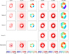 |
Fig. 6 Simulated polarized disk intensity and total disk intensity in different setups using the best fitting parameters, convolved with corresponding PSFs. Setup A assumes single dust species DIANA 0.01–1 μm dust in both the inner and outer disk. Setup Β has the same configuration as Setup A. but assumes single Henyey–Greenstein dust, with (ω, ɡ, pmax) = (0.32, 0.58, 0.37) at V-band and (0.69, 0.53, 0.58) at Ks-band. Setup C introduces a new cavity zone between the inner and outer disk. The inner disk and the cavity contains DIANA 0.01–0.1 μm dust. The outer disk contains the same dust as in Setup B. Setup D has the same configuration as C but assumes different dust in the rim and the spiral in the outer disk for the Ks band, (ω, ɡ, pmax) = (0.61, 0.47, 0.52) for the rim, and (0.79, 0.49, 0.74) for the spirals. |
Fitting results for the dust scattering parameters for each wavelength.
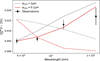 |
Fig. 7 Polarized flux integrated in the cavity region |

4.3 Setup C: New zone for cavity
To explain the V-band flux detected inside the cavity, which is not due to the convolution effect alone, we introduce a cavity zone to the model. The cavity is assumed to be geometrically aligned with the outer disk, supported by the inner-disk shadow matching the expected orientation in the outer ring; and optically thin with Mdust = 1.5 × 10⁻¹⁰Μ⊙, derived by adjusting the dust mass in RT model to match the observed V-band polarized flux.
The dust surface density in the cavity is described by Σ(r) ∝ r−ϵ exp[(r/Rtap)ϵ−2] with ϵ = −1 for a nearly flat surface density profile that gently decreases inward (see Fig. C.1). This choice is motivated by hydrodynamic simulations of the planet–disk interactions, where material inflow crosses a planet-carved gap and feeds the star, leading to a relatively uniform surface density inside the planet’s orbit (see Fig. 5 of Tatulli et al. 2011). Our adopted ϵ = −1 captures this behavior, and we find that small variations in ϵ have little impact on our modeling results.
Adding the optically thin dust in the cavity does not affect the outer disk appearance in the scattered light, so we fixed the outer disk parameters to those derived in Setup Β (Table 4 in this analysis. Since the inner disk is optically thick and unresolved, the dust species in the inner disk cannot be constrained so we assumed the same dust species as in the cavity.
In the optically thin cavity, the scattered light intensity is directly proportional to the scattering opacity κsca of the dust, which is primarily sensitive to the grain size distribution (Bohren & Huffman 1983). Therefore, the wavelength dependence of the cavity flux encodes information about dust size. However, we cannot reliably extract the total intensity in the cavity or apply PSF correction on  due to the faintness of the cavity signal and its proximity to the star. Instead, we adopt the forward-modeling approach: using the DIANA standard dust as a reference, we fix all parameters except for amax, and compare the convolved simulated polarized intensity
  to the observed value. This allowed us to simultaneously constrain the cavity dust properties and account for PSF smearing effects.
As shown in Fig. 7, the intrinsic  (gray dashed line) decreases with wavelength assuming DIANA standard dust. After convolution, the
  increases with wavelength (solid gray lines) due to the PSF smearing effect, however with a steeper gradient than the measurements. This mismatch indicates an even stronger wavelength dependence, i.e., a faster drop in the κsca(λ), is required to explain the observed cavity intensity. Such a trend can be achieved by reducing the maximum size, amax, in the size distribution, shifting the dust population closer to the Rayleigh regime κsca(λ) ∝ λ−4 if the wavelength dependence of the refractive index is negligible. A larger amax (>1 μm) results in an even steeper gradient in
  and can therefore be excluded. We found that reducing amax to 0.1 μm (red lines in Fig. 7) is enough to produce the observed trend. The simulated Qφ(x, y) maps for each wavelength are shown in Fig. 8. We see that in the intrinsic polarization, the cavity becomes fainter with wavelength. And the
  at Ks-band is mostly attributed to convolution effect.
The simulations with amax = 0.1 μm dust in the cavity are shown in Fig. 6 in the third row, reproducing the cavity signal. Even steeper spectral slopes can be realized by lowering amax further or by steepening the size distribution slope (p > 3.5), which makes the effective dust size even smaller. In any case, our results indicate that the scattering grains in the cavity cannot be larger than 0.1 μm. This is consistent with theoretical predictions of dust filtration, where large grains are trapped at the outer edge of a planet-induced gap and only small grains can flow inward (Zhu et al. 2012).
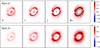 |
Fig. 8 Simulated polarized intensity maps in Setup C. Top row: intrinsic |


4.4 Setup D: Different dust species in spirals
In the previous setups, we assumed a uniform dust population across the outer disk. This is certainly an oversimplification, especially for a structured system such as HD 100453, where features such as the bright ring and trailing spirals may host different dust populations. Specifically, in the convolved Qφ-image, the spiral flux is underestimated by ~20%. In total intensity, the signal in spiral is reproduced by over-predicting the rim flux by ~10%. These discrepancies suggest a potential variation in dust properties. Therefore in Setup D, we explore this possibility by separating the dust population in the outer disk. We fix the inner disk and cavity components as in Setup C. We fit the HG dust parameters independently for the rim and the spirals, following a similar process as in Setup B.
For the rim, we chose seven observables: the integrated flux  ,
,  , the maximum polarization max(pdisk) and the brightness ratios RN/F and RN/M for both polarized and total intensity. The max(pdisk), RN/F, and RN/M are the same as measured for the whole disk. For the spiral, we chose five observables:
  ,
,  ,
,  and the brightness ratio
  and
and  . The Rsp acts as a near-far brightness ratio for the spiral, while the near side to major axis ratio is not available.
The independent fitting applies only for the Ks-band. This is not feasible for the V-band data because the spirals conincide with the strong speckle ring of the PSF and this noise introduces large uncertainties for the measured polarization of the spirals.
At Ks-band, the best-fitting parameters are (ω, ɡ, pmax) = (0.61 ± 0.03, 0.47 ± 0.02, 0.52 ± 0.04) for the rim, and (0.79 ± 0.02, 0.49 ± 0.04, 0.74 ± 0.06) for the spiral. The uncertainty represents 1σ deviation for the confidence interval of MCMC fitting. The convolved best-fitting model images are shown in Fig. 6 row Setup D. These results confirm that distinct dust properties in the spirals can better reproduce their brightness at Ks band. Compared to the global-fit parameters from Setup C, the rim values change only slightly, since the rim dominates the disk’s total brightness. The spiral region, however, favors higher ω and pmax values, suggesting more reflective grains with higher intrinsic polarization. This finding is discussed further in Section 5.2.
5 Discussion
5.1 Intrinsic disk polarization parameters
While the intrinsic disk-integrated azimuthal polarization  can be obtained directly from the observed data using a PSF-based correction map (Sect. 3.2), other parameters cannot be corrected in the same way because the convolution effects depend in a more complex way on the detailed structure of the disk. The RT modeling provides a high-quality nonconvolved simulation of both the disk total and polarized scattered light images, enabling accurate measurements of intrinsic values. In the following analysis, we adopt the best-fit models from Setup C for V-band and Setup D for Ks-band.
The full-disk intensity at Ks is not available from the observation due to the coronagraph. From model Setup D, we integrated the disk intensity and obtained Idisk/I★ = 4.2 ± 0.6% when integrating the convolved disk intensity in the elliptical region, and 4.8 ± 0.7% when integrating the intrinsic model. This difference arises because the PSF convolution spreads part of the disk signal into the central 0.125″ region, which lies inside the inner working angle and is excluded from the integration. Similarly for V-band, we integrated the unconvolved model and obtained Idisk/I★ = 1.5%. The uncertainty is assumed the same as for the coronagraphic image.
Previous measurements of the total intensity for HD 100453 have employed advanced imaging techniques and provided valuable measurements for comparison. For example, Long et al. (2017) reported disk-integrated fluxes of Idisk/I★ = 1.8 ± 0.1% at J and 2.5 ± 0.2% at H band using angular differential imaging (ADI) with KLIP (Soummer et al. 2012), which was among the first efforts to quantify the integrated scattered light in this system. While ADI techniques are known to introduce some level of self-subtraction for extended disk structures, these values fall neatly between our V- and Ks-band measurements, supporting a broadly consistent trend in the scattered light intensity across wavelengths. The K-hop data were presented by Ren et al. (2023) and high-quality extracted disk intensity image using NMF data imputation (Ren et al. 2020) was made publically available. Although the integrated disk flux was not reported in their work, we were able to re-analyze the image, correct for the coronagraphic transmission, and estimate Idisk/I★ = 3.4%, which only differs from our measurement by 10%. This is likely due to the inclusion of companion during PSF subtraction. Our improved flux estimates allow for more accurate and consistent measurements across filters, supporting further reliable color analysis.
Using the best-fit models at V (Setup C) and Ks (Setup D), we derive convolution-corrected fluxes for the rim and spirals separately in the concentric elliptical aperture, and the results are given in Table 5. The uncertainties are adopted from observed measurements. We also derived the corresponding degree of polarization maps and determined the intrinsic maximum polarization  . We find 40% at V and 55% at Ks-bands, higher than 28% and 39% earlier derived from the observed Qφ and Idisk maps directly. Since our convolved model reproduces the observed values well, this degradation of maximum degree of polarization must be attributed to the PSF convolution. The convolution smears the intensity and polarization, and further reduces the polarization signal by the mutual cancellation of the positive and negative components of the Stokes Q and U maps (Schmid & Ma 2025). While the disk-averaged degree of polarization 〈pdisk〉 at Ks is higher before correction, because the coronagraph partly hides the front side where the degree of polarization is low.
Color measurements. With these improved intrinsic flux measurements, we characterize the spectral dependence of disk reflectivity using the logarithmic color gradient  , where Ldisk corresponds to
  for ηΡΙ and Idisk/I★ for ηI (Tazaki et al. 2019). The colors are classified into blue (η < −0.5), gray (−0.5 < η < 0.5), and red (η > 0.5). For the HD 100453, we measure red color across V to Ks band, with a disk-integrated
  . More specifically, we find red colors both within the visible range
  and from visible to near-infrared
  , consistent with the earlier estimation from Ma et al. (2024), with significantly improved precision. Additionally in this work, we measure reddish-gray color in the infrared
  . When analyzing disk substructures, the rim shows a similar color to the full disk
  , while the spirals appear even redder, with
  . This redder trend in the spirals persists across other wavelength pairs as well.
Also for the total intensity, we estimate a red color  for the full disk. For substructures, we estimate
  and
and  , consistent with the full disk. Long et al. (2017) previously reported a bluer color in the spirals and interpreted this as evidence for smaller grains. While their result was based on ADI with KLIP, which is known to introduce self-subtraction biases in extended structures, our analysis yields a consistent red gradient across the disk. In particular, we find the spirals to be at least as red as the rim, if not redder. This suggests that the dust in the spirals is not necessarily smaller and could instead be shaped by other factors such as porosity or viewing geometry, which we’ll discuss in the following.
Measurements for observed and intrinsic disk radiation parameters for the V and Ks bands.
5.2 Dust species
The scattering parameters derived from forward model fitting assuming Henyey–Greenstein scattering show strong wavelength dependence from V to Ks bands. Specifically, the single scattering albedo ω increases from about 0.3 to 0.7, the asymmetry parameter remains around 0.5, and the maximum polarization pmax increases from about 0.4 to 0.6. These trends enable us to constrain the grain structure and composition on the disk surface.
5.2.1 Constraints with aggregate models
To interpret the derived scattering parameters in terms of dust structure, we turn to physically motivated aggregate dust models. We use the AggScatVIR (Aggregate Scattering for Visible and Infrared wavelengths) database (Tazaki et al. 2023), which provides a comprehensive library of light-scattering properties for aggregates with varying porosity, monomer size, and number of monomers, based on realistic collisional growth scenarios. Two compositions are considered: amc, a mixture of pyroxene silicate, water ice, troilite, and absorbent carbon; and org, which replaces the absorbent carbon with reflective carbon.
For all 360 models with power-law aggregate size distribution in AggScatVIR database, we calculated their scattering parameters (ω, ɡ, pmax). We begin by filtering and identifying dust models that show a moderate increase in pmax from V to Ks bands, as seen in our data. We focus on pmax because it is particularly sensitive to the dust structure and has been shown to strongly contain grain porosity and aggregate types (Tazaki & Dominik 2022; Tazaki et al. 2023). The filtering points to two promising amc families: CALP (compact aggregate with low porosity) models with 200 nm monomers and GRS (irregular grain).
To further investigate how individual dust properties influence the wavelength-dependent scattering behavior, we selected 14 representative models centered on these two families. In addition to the best-matching CALP and GRS models, we include variants where a single parameter – monomer size, porosity, or number of monomers – is altered. DIANA standard dust model used in Setup B is also included for comparison. Fig. 9 presents their scattering properties, where models are labeled as aggregate type_number of monomers_monomer size. The shaded region indicates the HG parameter ranges derived from our modeling (Table 5).
As shown in the third column of Fig. 9, irregular grains of volume equivalent radii aV ≈ 0.6–0.8 μm reproduce the observed increase in pmax the best. Compact aggregates composed of 200 nm monomers with similar volume equivalent radii aV also reproduce the trend. In contrast, more porous aggregates (e.g., CAMP, CAHP, and FA19, with porosity P > 70%) or smaller monomer size (e.g., CALP_32_100 nm) tend to over-predict the pmax(λ) gradient, and pmax value in the near-infrared, which is inconsistent with our observations. Larger dust aV > 1 μm does not show pmax increase.
Secondly, to evaluate if the candidates can also reproduce the observed red color, we adopted the effective albedo as defined in Mulders et al. (2013) to account for the inclined disk geometry:
 (10)
(10)
where θ represents the scattering angle, and the integration limits are set to [θ1, θ2] = [50°, 130°] in this study. The results are shown in the first column of Fig. 9.
While we did not search to fit the absolute ωeff values because the database has only two possible compositions, the increasing trend of ωeff(λ) is encouraging, as it suggests these aggregates can produce the observed red color in both the polarized and total disk reflectivity. The absolute value of ω mainly depends on the dust composition. In our models, the absorptive carbon species (amc) gives a reasonable match, though slightly increasing the fraction of more reflective components such as silicates and ices could improve the fit to the measurements. Still, what we really constrain is the refractive index, not the exact composition. Therefore, combinations with similar refractive indices as amc could produce the same scattering behavior.
Regarding the asymmetry parameter ɡ, all models show a decrease with wavelength, consistent with our observations, though ɡ(V) is generally higher than the HG fit. The volume-equivalent grain size appears to be the most critical factor, as models such as CALP_32_200 nm and grs_635nm reproduce ɡ values at both bands effectively. Increasing the grain size slightly (e.g., from 32_200nm to 128_200nm or from grs_400nm to grs_800nm) results in higher ɡ(Ks) values, leading to overly forward-scattering behavior in the Ks band. Sub-micron-sized dust give a marginally good match, while porosity and composition appear to have only secondary influence.
We also note that our observational constraints on ɡ are limited by the modest inclination of the system, which restricts us to a narrow range of scattering angles near 90°. This can bias estimates of ɡ derived from the observed brightness contrast (see discussion in Hughes et al. (2018) for a similar issue in debris disks). While our modeling captures general trends, we caution that redder colors could also arise from more isotropic scattering behavior or other geometric effects.
The AggScatVIR scattering properties serve as a first diagnostic tool, giving us insight into the types of aggregate structures that could explain our measured scattering parameters. As a final test, we validate these candidate aggregates by directly inserting them into RT simulations, comparing the predicted total disk color and degree of polarization against observations (Fig. 10). We find that CALP and GRS reproduce both red color and degree of polarization. By contrast, aggregates with higher porosity (𝒫>70%) can reproduce the red color, but overestimate the degree of polarization.
In summary, combining the initial filtering from the AggScatVIR database with full RT modeling, we conclude that the scattering properties in HD 100453’s surface layers are best explained by compact, low-porosity aggregates or irregular grains with volume-equivalent sizes around 0.8 μm.
Importantly, HD 100453 is a gas-depleted disk, with gas-to-dust ratios of 15–15 (van der Pias et al. 2019; Collins et al. 2009), which favors the existence of compact aggregates. Our results suggesting sub-micron, compact aggregates in the surface layer, could be interpreted as the evidence that the grains have undergone some dust processing. In contrast to gas-rich disks such as ΓΜ Lup, where fluffy, primordial aggregates are inferred (Tazaki et al. 2023), dust in HD 100453 appears more evolved. The low porosity might arise from collisional compaction or fragmentation in the low-gas environment (Tanaka et al. 2023; Michoulier et al. 2024). Additionally, the absence of large grains in the surface layer could reflect vertical settling in a disk with moderate turbulence, consistent with expectations for gas-depleted systems.
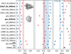 |
Fig. 9 Comparison of the scattering properties ωeff, ɡ, and pmax of selected dusts species from AggScatVIR database. The dusts are labeled by morphology_number of monomers_monomer size. The morphology includes compact aggregates CALP (low porosity), CAMP (medium porosity), and CAHP (high porosity) and fractal aggregates FA19 (df=1.9), further characterized by the number of monomers and monomer sizes in nanometers. Irregular grains (GRS) are characterized by volume equivalent radii. If not specified, the composition amc is used. CALP_32_200 nm and grs_635 nm examples are placed to show their morphology. |
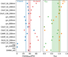 |
Fig. 10 Comparison of max(pdisk) (left column) and disk-integrated colors ηV/K (right column) when assuming different dust species from AggScatVIR database. The label convention is the same as in Fig. 9. |
5.2.2 Substructure-dependent dust scattering behavior
The origin of the spirals in HD 100453 has long been debated, with popular explanations including shadows cast by a misaligned inner disk (Benisty et al. 2017) and tidal perturbations from the stellar companion(Wagner et al. 2018; van der Pias et al. 2019). While both scenarios are plausible, recent kinematic measurements using high-resolution ALMA and SPHERE imaging favor the companion-driven origin (Rosotti et al. 2020; Xie et al. 2023). However, how these spirals influence dust evolution remains unclear. Existing simulations explored dust dynamics in both scenarios (Cuello et al. 2019; Gonzalez et al. 2020; Nealon et al. 2020), but they were not designed to interpret the Polarimetrie scattered light images. The simulations followed the gas and dust evolution and predicted grain size distributions, but the dust is typically treated with Mie theory assuming astrosilicates. Introducing more realistic grains, especially nonspherical grains, would improve future comparisons with observations to study how dust evolution varies across substructures.
Our analysis reveals a higher maximum degree of polarization pmax in spirals than the main ring at Ks band, suggesting dust grains in the spirals are more porous or smaller. This trend is robust against geometric uncertainties, as pmax is insensitive to moderate changes in scattering surface height. To test the effect of geometry, we varied the spiral scale height in the RT model. Increasing the height modestly shifts the best-fit scattering parameters (e.g., increasing both ω and ɡ), but does not affect pmax significantly. Therefore, while the absolute values may depend on geometry, the relative enhancement of pmax in the spirals is likely intrinsic to the dust. The elevated pmax in the spirals is consistent with compact aggregates of lower porosity in the ring and slightly more porous grains in the spirals. These findings highlight the potential of spiral arms to show differential grain growth, waiting for further investigation with physically consistent grain evolution models.
The cavity region also shows a distinctly different dust population. Our forward modeling indicates that only small grains (amax ≲ 0.1 μm) can reproduce the observed steep drop in polarized flux with wavelength. This supports a scenario where large grains are filtered out at the cavity edge, consistent with theoretical expectations of planet-induced dust filtration (Zhu et al. 2012; Pinilla et al. 2016), where the gas is still present (van der Plas et al. 2019). These results highlight the potential to reveal a small grain population and provide new evidence of dust filtration in other transition disks with gas-filled cavities (e.g., HD 135344B, Carmona et al. 2014) by including short-wavelength PDI observations in future studies.
6 Conclusions
We have presented new polarimetric observations of HD 100453 at the V, I′, J, and Ks bands. We considered the PSF convolution effects and corrected for the cancellation in Qφ-images to measure the intrinsic, integrated polarized flux. We performed reference differential imaging in star-hopping observing sequences at the V and Ks bands to extract total disk intensity images. We demonstrated that reference differential imaging is also applicable to ZIMPOL observations in the V-band, and we improved the disk intensity extraction at the Ks-band. We measured the integrated disk intensity, Idisk, and derived a red color. We recognized an intrinsic scattering signal in the cavity in V and I′ images. We also measured a brightness ratio between the near and far side, which decreases with wavelength.
We then characterized the dust properties using the radiative transfer RADMC-3D disk model with four different setups. Reproducing the simulation of Benisty et al. (2017) using the DIANA standard dust model revealed a deficit on the total and polarized disk flux in the Ks-band observations. Adopting Henyey–Greenstein scattering phase functions for the dust reproduced the observation at both wavelengths, with best-fitting scattering parameters (ω, ɡ, pmax) varying from (0.32, 0.58, 0.37) at V to (0.69, 0.53, 0.58) at Ks. The dust dominating the upper layer of the disk is most likely composed of sub-micron-sized low-porosity aggregates and/or irregular grains. Introducing dust in the cavity zone between the inner and outer disks, we characterized the maximum dust size, amax < 0.1 μm, by fitting the cavity flux as a function of wavelength. Finally, we found that the dust in the spirals produces a higher scattering polarization, pmax, when compared to regions further in, hinting at more porous or smaller dust.
The results pointing to different dust species across the disk reflect distinct dust formation and evolution processes, such as grain growth in spirals versus the main ring and dust filtration at cavity edges. Linking these properties to specific mechanisms offers valuable insight into planet formation. Future studies that will expand the sample to a larger number of disks will be essential for identifying common patterns and constraining the physical processes shaping protoplanetary environments.
Data availability
The reduced Qφ images in Fig. 1 and extracted disk intensity Idisk maps in Fig. 3 are available at the CDS via https://cdsarc.cds.unistra.fr/viz-bin/cat/J/A+A/702/A78.
Acknowledgement
We thank the anonymous referee for the valuable comments on the manuscript. We thank Andrés Carmona González for helpful discussions on the surface density setups. We are also grateful to Bin Ren for his input on disk intensity extraction, and to Anthony Boccaletti for providing the coronagraphic transmission profiles. J.M. thanks the Swiss National Science Foundation for financial support under grant number P500PT_222298. R.T. is supported by JSPS KAKENHI Grant Numbers JP25K07351. G.D. and F.M. acknowledge funding from the European Research Council (ERC) under the European Union’s Horizon Europe research and innovation program (grant agreement No. 101053020, project Dust2Planets.)
Appendix A Photometric calibrations
A.1 Background subtraction
The thermal background noise is known to be an issue for Ks band observation (Beuzit et al. 2019), not important at shorter wavelengths. Therefore, we applied background subtraction to Ks band PSF images. For K-hop sequence, sky images were taken only for saturated object frames but not for flux frames for Ks deep observing sequences. Therefore, although the pipeline estimates and subtracts a flat background signal in a large annulus, the lack of sky images still results in a background in the reduced images, see Fig. A.1 top left image. In addition, a faint ghost is seen, while the companion is not visible in this short exposure. Similarly, no sky images were taken for K-sequence, which results in nonnegligeable background signal, as shown in Fig. A.1 bottom left image. The companion is well-visible in the SE direction.
For K-hop, we performed a second-order polynomial fitting to the background in the two Ileft and Iright images. The long-exposures have sky-frames so Q and U are also not affected. For Κ sequence, we performed a linear fitting to the background in the radial direction for each cycle of Itot images. The background is at the same level for all frames so Q and U images are not affected. The background-subtracted images are shown in the middle column of Fig. A.1. This step is important for an accurate quantitative measurement of integrated stellar flux I★.
After the background subtraction, we filtered the ghost on the west for K-hop and the companion for K. The flux frames after the background subtraction and ghost/companion filtering are present on the right columns of Fig. A.1.
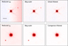 |
Fig. A.1 Example of background subtraction and companion/ghost filtration. Top left: Ileft image of flux frame taken before all Polarimetrie cycles in K-hop. Top middle: Ileft with the background subtracted. Top right: Ileft with the background subtracted and with the ghost filtered. Bottom left: Itot of the first cycle from the Κ sequence. Bottom middle: Itot with the background subtracted. Bottom right: Itot with the background subtracted and the companion filtered. |
A.2 Coronagraph transmission correction
The coronagraph N_ALC_Ks combines the apodizer and the Lyot stop of diameter 0.24″. Although the suggested inner working angle (IWA) in the manual is r = 0.2″, we tried to recover the intensity close to 0.125″ using the radial transmission curve1. We interpolated the curve and corrected the flux between 0.125″ and 0.5″, as shown in Fig. A.2 left panel. We consider the IWA = 0.125″ at which the transmission is 50%, indicated in Fig. A.2 as the white dashed line, and discard the data inward. Then for each image frame, we corrected the transmission by dividing T(x, y) pixel-wise. In the right panel, we show the radial profiles of the total intensity Idisk(r) on the near and far sides. The profiles are normalized to the peak value on the major axis, and the far side is shifted by 2 for clarity.
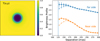 |
Fig. A.2 Coronagraph N_ALC_Ks transmission correction. Left: Transmission map T(x, y) of coronagraph N_ALC_Ks zoomed to 1×1″. Right: Radial profile of the total disk intensity Idisk(r) for the near and far sides. The dashed and solid lines represent the profiles before and after the correction respectively. |
This correction is important for HD 100453 not only for integrated flux but also for brightness ratios. Outside the IWA, the correction is well characterized and improves the flux estimates. Without applying transmission correction, the integrated flux Idisk/I★ = 3.5% and  , meaning 20% and 6% flux underestimation in Idisk and Qφ respectively. Since the main correction is on the near and far side of the disk, and near side loses more flux as it is closer to the center from projection effect, the RN/F and RN/M will be underestimated in both the polarized intensity and total intensity if not corrected. The coronagraph also pushes the peak intensity outward or even creates an artificial peak.
A.3 Flux of companion
To estimate the relative flux ratio between the host star and the companion, we performed aperture photometry using circular aperture r = 0.1″ with local background estimated in the surrounding annulus r = [0.10, 0.11]″. We integrate the flux for the companion  and for the star
  for each cycle. Since the companion is too faint in V-band short exposures, we do not have simultaneous unsaturated A and Β at this wavelength. We measure
  in long exposures and
  in short exposures separately. For I, J, and Ks, unsaturated star A and Β are clearly visible in each total intensity frame, and we calculate the flux ratio
  cycle by cycle. The results are summarized in Table A.1.
Then we adopt the magnitude mA for HD 100453 A(Høg et al. 2000; Cutri et al. 2003; ESA 1997) and derive the magnitude of HD 100453 Β, including the first magnitude value at J-band. The mB at V agree with previous studies in Collins et al. (2009), which measured mB = 15.88 using HST F606W image. We did not include mB at Ks because the inner disk largely contributes to the central radiation at Ks (Khalafinejad et al. 2016), and the disk intensity might be variable making IA at this wavelength not a reliable reference to determine mB.
Flux and magnitude of the companion HD 100453B.
Appendix B Disk intensity extraction
B.1 Halo component
Including the halo component in RDI is necessary for V band. To first-order approximation, the scaling factor in Eq. (3) can be estimated as a ≈ ΣΙ★/ΣΙref, where Σ denotes integration over a disk-free region. However, if the selected fitting region is contaminated by extended disk signal (i.e., the halo component Igaio), which is often the case, the effective scaling becomes a′ ≈ Σ(I★ + Ihalo)/ΣIref > a, thus overestimating the scaling factor by Δa = ΣIhalo/ΣIref.
When applied to the subtraction on the disk region, this leads to oversubtraction of the disk signal at each pixel ΔIdisk(x, y) = Δa · Iref(x, y). This oversubtraction becomes significant when the relative error,
 (B.1)
(B.1)
is nonnegligible. Thus, even a small amount of halo contamination can lead to large errors if the disk signal is faint relative to the reference.
Using the Setup A model at V band, we calculated the radial profile Idisk(r) and fitted the halo profile in r = [0.43, 0.76]″ with an exponential drop-off, resulting in Idisk(r) ∝ e−4 5 r.
We estimated ΣIhalo/ΣIref ≈ 1% in the chosen fitting region and Iref / Idisk(x, y) ≈ 20 at the disk intensity peak location. This implies that neglecting the halo component leads to about 20% underestimation of the Idisk(x, y) at peak position. The extracted disk intensity ignoring this halo component is plot in the left panel of Fig. B.1, clearly showing the oversubstraction.
For comparison, we applied the same estimation to Ks-band. We find ΣIhalo/ΣIref ≈ 4% in the chosen fitting region, but Iref/Idisk(x, y) ≈ 0.5 at the peak of the disk because the disk is brighter and the star is fainter at longer wavelength. This results in only a 2% underestimation of the Idisk. Therefore, we consider the contribution of Ihalo as negligible at the Ks-band.
B.2 Excluding companion
Although the Ks band disk intensity extraction does not suffer from the extended disk halo created by the convolution effect, including the companion into the fitting region results in a similar effect. This effect is seen when we compare our results with that from Ren et al. (2023), where a faint negative halo present because of including the companion into the fitting region. Therefore, the disk intensity is oversubtracted, and the disk signal is underestimated. We followed the steps as described in Ren et al. (2023), but using the imputation mask excluding the companion (indicated by the gray shaded region in Fig. B.1). We also applied the transmission correction as described in Appendix. A.2 and the result is shown in Fig. B.1 right panel. We see that the improved data imputation result is comparable to the classic RDI (shown in Fig. 3), integrating to Idisk/I★ = 3.86% agrees well with our results using classic RDI.
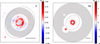 |
Fig. B.1 Fitting region, Σ, used for disk intensity extraction. Left: Fitting region at V-band. The gray shaded annulus indicates Σ, overplotted on Idisk(x, y)(V) extracted without introducing halo component. Right: Fitting region at Ks band. The gray shaded region indicates Σ at Ks-band, overplotted on Idisk(x, y)(K) extracted using NMF_imaging with improved Σ. The two images are shown in different scales to highlight the Σ, with the black bar indicating 0.5″. The gray dashed lines encloses the region for disk intensity integration. |
In summary, we conclude that false-flagging pixels containing disk signal or any other contamination in the fitting region or the data imputation can be dangerous. When we adopt the same good fitting region in our case of HD 100453, the classic RDI and the data imputation results agree pretty well.
Appendix C Model parameters
The model parameters used in the RADMC-3D model are summarized in Table C.1. The model is built based on the description in Benisty et al. (2017). The main difference lies in the adjustment of spiral geometry and the new cavity zone. The spiral geometry parameters are slightly modified (highlighted in Table C.1) mostly because we ignore the dust settling in this study. The new cavity zone only appears in Setups C and D, with its profile shown in Fig. C.1.
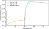 |
Fig. C.1 Surface density used in the radiative transfer model. |
RADMC-3D model parameters used in this work.
References
- Benisty, M., Stolker, T., Pohl, A., et al. 2017, A&A, 597, A42 [NASA ADS] [CrossRef] [EDP Sciences] [Google Scholar]
- Benisty, M., Dominik, C., Follette, K., et al. 2023, in Astronomical Society of the Pacific Conference Series, 534, Protostars and Planets VII, eds. S. Inutsuka, Y. Aikawa, T. Muto, K. Tomida, & M. Tamura, 605 [NASA ADS] [Google Scholar]
- Beuzit, J. L., Vigan, A., Mouillet, D., et al. 2019, A&A, 631, A155 [NASA ADS] [CrossRef] [EDP Sciences] [Google Scholar]
- Birnstiel, T. 2024, ARA&A, 62, 157 [NASA ADS] [CrossRef] [Google Scholar]
- Bohren, C. F., & Huffman, D. R. 1983, Absorption and Scattering of Light by Small Particles (New York: Wiley) [Google Scholar]
- Carmona, A., Pinte, C., Thi, W. F., et al. 2014, A&A, 567, A51 [NASA ADS] [CrossRef] [EDP Sciences] [Google Scholar]
- Collins, K. A., Grady, C. A., Hamaguchi, K., et al. 2009, ApJ, 697, 557 [NASA ADS] [CrossRef] [Google Scholar]
- Cuello, N., Montesinos, M., Stammler, S. M., Louvet, F., & Cuadra, J. 2019, A&A, 622, A43 [NASA ADS] [CrossRef] [EDP Sciences] [Google Scholar]
- Cutri, R. M., Skrutskie, M. F., van Dyk, S., et al. 2003, VizieR On-line Data Catalog: II/246 [Google Scholar]
- Dipierro, G., Pinilla, P., Lodato, G., & Testi, L. 2015, MNRAS, 451, 974 [Google Scholar]
- Dullemond, C. P., Juhasz, A., Pohl, A., et al. 2012, RADMC-3D: A multipurpose radiative transfer tool, Astrophysics Source Code Library [record ascl:1202.015] [Google Scholar]
- ESA 1997, The HIPPARCOS and TYCHO catalogues. Astrometric and photometric star catalogues derived from the ESA HIPPARCOS Space Astrometry Mission, ESA Special Publication, 1200 [Google Scholar]
- Foreman-Mackey, D., Hogg, D. W., Lang, D., & Goodman, J. 2013, PASP, 125, 306 [Google Scholar]
- Gaia Collaboration (Vallenari, A., et al.) 2023, A&A, 674, A1 [NASA ADS] [CrossRef] [EDP Sciences] [Google Scholar]
- Garcia, A. J. L., & Gonzalez, J.-F. 2020, MNRAS, 493, 1788 [Google Scholar]
- Gonzalez, J.-F., van der Plas, G., Pinte, C., et al. 2020, MNRAS, 499, 3837 [Google Scholar]
- Henyey, L. G., & Greenstein, J. L. 1941, ApJ, 93, 70 [Google Scholar]
- Høg, E., Fabricius, C., Makarov, V. V., et al. 2000, A&A, 355, L27 [Google Scholar]
- Hughes, A. M., Duchêne, G., & Matthews, B. C. 2018, ARA&A, 56, 541 [Google Scholar]
- Khalafinejad, S., Maaskant, K. M., Mariñas, N., & Tielens, A. G. G. M. 2016, A&A, 587, A62 [NASA ADS] [CrossRef] [EDP Sciences] [Google Scholar]
- Long, Z. C., Fernandes, R. B., Sitko, M., et al. 2017, ApJ, 838, 62 [Google Scholar]
- Ma, J., & Schmid, H. M. 2022, A&A, 663, A110 [NASA ADS] [CrossRef] [EDP Sciences] [Google Scholar]
- Ma, J., Schmid, H. M., & Stolker, T. 2024, A&A, 683, A18 [NASA ADS] [CrossRef] [EDP Sciences] [Google Scholar]
- Malfait, K., Bogaert, E., & Waelkens, C. 1998, A&A, 331, 211 [NASA ADS] [Google Scholar]
- Meeus, G., Waters, L. B. F. M., Bouwman, J., et al. 2001, A&A, 365, 476 [CrossRef] [EDP Sciences] [Google Scholar]
- Michoulier, S., Gonzalez, J.-F., & Price, D. J. 2024, A&A, 688, A31 [NASA ADS] [CrossRef] [EDP Sciences] [Google Scholar]
- Min, M., Hovenier, J. W., & de Koter, A. 2005, A&A, 432, 909 [NASA ADS] [CrossRef] [EDP Sciences] [Google Scholar]
- Min, M., Dullemond, C. P., Dominik, C., de Koter, A., & Hovenier, J. W. 2009, A&A, 497, 155 [NASA ADS] [CrossRef] [EDP Sciences] [Google Scholar]
- Min, M., Rab, C., Woitke, P., Dominik, C., & Ménard, F. 2016, A&A, 585, A13 [NASA ADS] [CrossRef] [EDP Sciences] [Google Scholar]
- Mulders, G. D., Min, M., Dominik, C., Debes, J. H., & Schneider, G. 2013, A&A, 549, A112 [NASA ADS] [CrossRef] [EDP Sciences] [Google Scholar]
- Nealon, R., Cuello, N., Gonzalez, J.-F., et al. 2020, MNRAS, 499, 3857 [Google Scholar]
- Pinilla, P., Klarmann, L., Birnstiel, T., et al. 2016, A&A, 585, A35 [NASA ADS] [CrossRef] [EDP Sciences] [Google Scholar]
- Ren, B., Pueyo, L., Chen, C., et al. 2020, ApJ, 892, 74 [Google Scholar]
- Ren, B. B., Benisty, M., Ginski, C., et al. 2023, A&A, 680, A114 [NASA ADS] [CrossRef] [EDP Sciences] [Google Scholar]
- Rosotti, G. P., Benisty, M., Juhász, A., et al. 2020, MNRAS, 491, 1335 [Google Scholar]
- Schmid, H. M., & Ma, J. 2025, A&A, submitted [Google Scholar]
- Schmid, H. M., Bazzon, A., Roelfsema, R., et al. 2018, A&A, 619, A9 [NASA ADS] [CrossRef] [EDP Sciences] [Google Scholar]
- Soummer, R., Pueyo, L., & Larkin, J. 2012, ApJ, 755, L28 [Google Scholar]
- Tanaka, H., Anayama, R., & Tazaki, R. 2023, ApJ, 945, 68 [NASA ADS] [CrossRef] [Google Scholar]
- Tatulli, E., Benisty, M., Ménard, F., et al. 2011, A&A, 531, A1 [NASA ADS] [CrossRef] [EDP Sciences] [Google Scholar]
- Tazaki, R., & Dominik, C. 2022, A&A, 663, A57 [NASA ADS] [CrossRef] [EDP Sciences] [Google Scholar]
- Tazaki, R., Tanaka, H., Muto, T., Kataoka, A., & Okuzumi, S. 2019, MNRAS, 485, 4951 [NASA ADS] [CrossRef] [Google Scholar]
- Tazaki, R., Ginski, C., & Dominik, C. 2023, ApJ, 944, L43 [NASA ADS] [CrossRef] [Google Scholar]
- Tschudi, C., & Schmid, H. M. 2021, A&A, 655, A37 [NASA ADS] [CrossRef] [EDP Sciences] [Google Scholar]
- van der Plas, G., Ménard, F., Gonzalez, J. F., et al. 2019, A&A, 624, A33 [NASA ADS] [CrossRef] [EDP Sciences] [Google Scholar]
- van Holstein, R. G., Girard, J. H., de Boer, J., et al. 2020, IRDAP: SPHERE-IRDIS Polarimetrie data reduction pipeline, Astrophysics Source Code Library, [record ascl:2004.015] [Google Scholar]
- Wagner, K., Apai, D., Kasper, M., & Robberto, M. 2015, ApJ, 813, L2 [Google Scholar]
- Wagner, K., Dong, R., Sheehan, P., et al. 2018, ApJ, 854, 130 [Google Scholar]
- Wahhaj, Z., Milli, J., Romero, C., et al. 2021, A&A, 648, A26 [EDP Sciences] [Google Scholar]
- Woitke, P., Min, M., Pinte, C., et al. 2016, A&A, 586, A103 [NASA ADS] [CrossRef] [EDP Sciences] [Google Scholar]
- Xie, C., Ren, B. B., Dong, R., et al. 2023, A&A, 675, L1 [NASA ADS] [CrossRef] [EDP Sciences] [Google Scholar]
- Zhu, Z., Nelson, R. P., Dong, R., Espaillat, C., & Hartmann, L. 2012, ApJ, 755, 6 [Google Scholar]
See section A.6 from SPHERE user manual at https://www.eso.org/sci/facilities/paranal/instruments/sphere/doc/VLT-MAN-SPH-14690-0430_P114_july_2024_zwa.pdf
All Tables
Observed polarized flux Qφ/Ι★ integrated in different apertures for HD 100453 for each observing date.
Measurements for observed and intrinsic disk radiation parameters for the V and Ks bands.
All Figures
|
Fig. 1 Polarized intensity images Qφ(x,y) and Uφ(x,y) for V, I′, J, and Ks band. All images are normalized to the integrated stellar intensity I★ and their pixel scale (3.6 × 3.6 mas2 for ZIMPOL and 12.25 × 12.25 mas2 for IRDIS). The shared color bar is indicated on the right. All the images are cut to 1.0 × 1.0″ and the black bar in Qφ(V) indicates 0.2″. The dashed lines in Uφ(V) enclose the integration region for the cavity, the rim, and the spiral respectively. The semitransparent circle in K-hop represents the inner working angle (IWA) = 0.125″ limited by the coronagraph. North is up and east to the left. |
| In the text | |
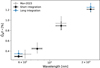 |
Fig. 2 Intrinsic integrated polarized flux |
| In the text | |
|
Fig. 3 Extracted disk intensity map Idisk(x, y) for the V- and Ks-bands, cut to 2.0 × 2.0″. The black bar indicates 0.5″. The central 0.1″ and 0.125″ are masked out as the IWA for V and Ks respectively. |
| In the text | |
|
Fig. 4 Observed degree of polarization pdisk(x, y) for V- and Ks-bands cut to 1.0 × 1.0″. The black bar in the V-band subfigure indicates 0.2″. The star marker indicates the position of the central host star. |
| In the text | |
|
Fig. 5 Radial profiles of polarized intensity Qφ(r) along both sides of the major axis (left), near side (middle), and far side (right). All profiles have been normalized to the peak value along the major axis and shifted by one for clarity. The standard deviation among all cycles at a given epoch is indicated as the error bar. The shaded region indicates the cavity region [0.10, 0.13]″. |
| In the text | |
|
Fig. 6 Simulated polarized disk intensity and total disk intensity in different setups using the best fitting parameters, convolved with corresponding PSFs. Setup A assumes single dust species DIANA 0.01–1 μm dust in both the inner and outer disk. Setup Β has the same configuration as Setup A. but assumes single Henyey–Greenstein dust, with (ω, ɡ, pmax) = (0.32, 0.58, 0.37) at V-band and (0.69, 0.53, 0.58) at Ks-band. Setup C introduces a new cavity zone between the inner and outer disk. The inner disk and the cavity contains DIANA 0.01–0.1 μm dust. The outer disk contains the same dust as in Setup B. Setup D has the same configuration as C but assumes different dust in the rim and the spiral in the outer disk for the Ks band, (ω, ɡ, pmax) = (0.61, 0.47, 0.52) for the rim, and (0.79, 0.49, 0.74) for the spirals. |
| In the text | |
|
Fig. 7 Polarized flux integrated in the cavity region |
| In the text | |
|
Fig. 8 Simulated polarized intensity maps in Setup C. Top row: intrinsic |
| In the text | |
|
Fig. 9 Comparison of the scattering properties ωeff, ɡ, and pmax of selected dusts species from AggScatVIR database. The dusts are labeled by morphology_number of monomers_monomer size. The morphology includes compact aggregates CALP (low porosity), CAMP (medium porosity), and CAHP (high porosity) and fractal aggregates FA19 (df=1.9), further characterized by the number of monomers and monomer sizes in nanometers. Irregular grains (GRS) are characterized by volume equivalent radii. If not specified, the composition amc is used. CALP_32_200 nm and grs_635 nm examples are placed to show their morphology. |
| In the text | |
|
Fig. 10 Comparison of max(pdisk) (left column) and disk-integrated colors ηV/K (right column) when assuming different dust species from AggScatVIR database. The label convention is the same as in Fig. 9. |
| In the text | |
|
Fig. A.1 Example of background subtraction and companion/ghost filtration. Top left: Ileft image of flux frame taken before all Polarimetrie cycles in K-hop. Top middle: Ileft with the background subtracted. Top right: Ileft with the background subtracted and with the ghost filtered. Bottom left: Itot of the first cycle from the Κ sequence. Bottom middle: Itot with the background subtracted. Bottom right: Itot with the background subtracted and the companion filtered. |
| In the text | |
|
Fig. A.2 Coronagraph N_ALC_Ks transmission correction. Left: Transmission map T(x, y) of coronagraph N_ALC_Ks zoomed to 1×1″. Right: Radial profile of the total disk intensity Idisk(r) for the near and far sides. The dashed and solid lines represent the profiles before and after the correction respectively. |
| In the text | |
|
Fig. B.1 Fitting region, Σ, used for disk intensity extraction. Left: Fitting region at V-band. The gray shaded annulus indicates Σ, overplotted on Idisk(x, y)(V) extracted without introducing halo component. Right: Fitting region at Ks band. The gray shaded region indicates Σ at Ks-band, overplotted on Idisk(x, y)(K) extracted using NMF_imaging with improved Σ. The two images are shown in different scales to highlight the Σ, with the black bar indicating 0.5″. The gray dashed lines encloses the region for disk intensity integration. |
| In the text | |
|
Fig. C.1 Surface density used in the radiative transfer model. |
| In the text | |
Current usage metrics show cumulative count of Article Views (full-text article views including HTML views, PDF and ePub downloads, according to the available data) and Abstracts Views on Vision4Press platform.
Data correspond to usage on the plateform after 2015. The current usage metrics is available 48-96 hours after online publication and is updated daily on week days.
Initial download of the metrics may take a while.