| Issue |
A&A
Volume 702, October 2025
|
|
|---|---|---|
| Article Number | A64 | |
| Number of page(s) | 11 | |
| Section | Cosmology (including clusters of galaxies) | |
| DOI | https://doi.org/10.1051/0004-6361/202556332 | |
| Published online | 07 October 2025 | |
RedMaPPer cluster properties from two-dimensional lensing shear maps in the HSC-SSP survey
1
South-Western Institute for Astronomy Research (SWIFAR), Yunnan University, Kunming 650500, PR China
2
Yunnan Key Laboratory of Survey Science,Yunnan University, Kunming 650500, PR China
3
Shanghai Astronomical Observatory (SHAO), Nandan Road 80, Shanghai 200030, PR China
4
University of Chinese Academy of Sciences, Beijing 100049, PR China
⋆ Corresponding authors: This email address is being protected from spambots. You need JavaScript enabled to view it.
; This email address is being protected from spambots. You need JavaScript enabled to view it.
Received:
9
July
2025
Accepted:
21
August
2025
Abstract
Context. Dark matter halos are fundamental structures in the Universe and serve as crucial cosmological probes. Key properties of halos–such as their concentration, ellipticity, and mass centroid–encode valuable information about their formation and evolutionary history. In particular, halo concentration reflects the collapse time and internal structure of halos, while measurements of ellipticity and centroid positions provide insights into the shape and dynamical state of halos. Moreover, accurately characterizing these properties is essential for improving mass estimates and for testing models of dark matter. Gravitational lensing, which directly probes the projected mass distribution without relying on assumptions about the dynamical state, has emerged as a powerful observational tool to constrain these halo properties with high precision.
Aims. We aim to derive precise constraints on key structural properties of galaxy clusters–including halo concentration, ellipticity, and the position of mass centroids–by directly fitting observed two-dimensional (2D) weak-lensing shear maps with elliptical Navarro–Frenk–White (NFW) models. These measurements help to reveal the internal structure of massive clusters and to quantify systematic uncertainties in stacked lensing analyses.
Methods. We performed a 2D weak-lensing analysis of 299 massive clusters selected from the redMaPPer catalog, using shear measurements from the first-year data release of the Hyper Suprime-Cam Subaru Strategic Program (HSC-SSP). Elliptical NFW profiles were fit to the shear maps with Gaussian priors on the halo mass calibrated from the redMaPPer cluster richness–mass relation. These priors serve to break the mass–concentration degeneracy in the statistical modeling and, to some extent, tighten the constraints on the other parameters of primary interest.
Results. The derived concentration–mass relation exhibits a slightly steeper slope than traditional weak-lensing power-law or upturn models, and agrees more closely with the results from strong lensing selected halos. More massive and lower-redshift clusters tend to have lower concentrations and appear more spherical. The halo ellipticity distribution is characterized by e = 1 − b/a = 0.530 ± 0.168, with a mean of ⟨e⟩ = 0.505 ± 0.007. We also detect a bimodal distribution in the offsets between optical centers and mass centroids: some halos are well aligned with their brightest cluster galaxy (BCG), while others show significant displacements. These results highlight the power of 2D weak-lensing modeling in probing halo morphology and in providing key inputs for understanding and modeling systematic effects in stacked lensing analyses.
Key words: gravitational lensing: weak / methods: statistical / galaxies: clusters: general / cosmology: observations / dark matter
© The Authors 2025
 Open Access article, published by EDP Sciences, under the terms of the Creative Commons Attribution License (https://creativecommons.org/licenses/by/4.0), which permits unrestricted use, distribution, and reproduction in any medium, provided the original work is properly cited.
This article is published in open access under the Subscribe to Open model. This email address is being protected from spambots. You need JavaScript enabled to view it. to support open access publication.
1. Introduction
The formation of large-scale structures in the Universe, predicted by N-body simulations based on the Λ cold dark matter (ΛCDM) cosmological model, follows a “bottom-up” process. In this scenario, smaller structures form first and gradually merge into larger ones under the influence of gravity. These hierarchical structures make up the cosmic web (Zel’dovich 1970), where significant concentrations of matter accumulate at the intersections, leading to the formation of massive dark matter (DM) halos. They host the formation of galaxy clusters, with lower-mass halos mainly merging along filamentary structures (Peebles 1980). Galaxy clusters, the largest self-gravitationally bound systems observed, play a critical role in shaping the formation and evolution of the Universe. Therefore, studying the properties of these clusters would provide crucial insights into the growth of cosmic structures and the nature of DM.
The key properties that characterize galaxy clusters, such as the halo mass function (e.g., Press & Schechter 1974; Sheth & Tormen 1999; Jenkins et al. 2001; Tinker et al. 2008; Watson et al. 2013) and the density profile (e.g., Navarro et al. 1997; Bullock et al. 2001; Macciò et al. 2007; Duffy et al. 2008; Mandelbaum et al. 2008; Ludlow et al. 2016; Shan et al. 2017; Child et al. 2018), can be used to test and refine our understanding of structure formation and the evolution of large-scale structures, and are thus essential for constraining cosmological models (Ghirardini et al. 2024). A variety of methods have been developed to measure the properties of halos, each with its strengths and limitations. X-ray observations, for example, allow for the measurement of the total mass of clusters based on the temperature and flux profiles of the hot gas assuming spherical symmetry and hydrostatic equilibrium (Nagai et al. 2007), which can introduce biases in clusters that deviate from spherical shapes and equilibrium. The Sunyaev-Zel’dovich (SZ) effect links the ionized gas in clusters with cosmic microwave background (CMB) observations, and provides crucial, redshift-independent observables that directly probe the integrated electron pressure of the intracluster medium, enabling us to derive fundamental cluster properties such as the mass and thermodynamic state of galaxy clusters across cosmic time (Planck Collaboration XXIV 2016). However, point sources and foreground signals could contaminate the SZ effect and complicate the measurements (Carlstrom et al. 2002; Vale & White 2006). Other methods, such as dynamics-based estimates, focus on galaxy velocity dispersion and distribution (Brainerd 2005; Sohn et al. 2020), but are also sensitive to the galaxy population within clusters (Nagai & Kravtsov 2005).
Weak gravitational lensing (WL) provides an independent and powerful method of studying galaxy clusters. Unlike other techniques, WL does not rely on assumptions about the hydrodynamic state or symmetry of the clusters (e.g., Shan et al. 2018; Li et al. 2023a). The lensing effect arises when the light from background galaxies is distorted due to the gravitational field of massive foreground structures, including galaxy clusters (Bartelmann & Schneider 2001; Hoekstra & Jain 2008; Fu & Fan 2014; Kilbinger 2015; Schrabback et al. 2025; Diego et al. 2025). These distortions thus offer a direct way to probe the distribution of DM in the clusters and provide valuable information about their mass, shape, and orientation. Recent WL surveys, including the Canada–France Hawaii Telescope Lensing Survey (CFHTLenS1; Heymans et al. 2012), the Dark Energy Survey (DES2; Dark Energy Survey Collaboration 2016), the Kilo-Degree survey (KiDS3; de Jong et al. 2013), the Hyper Suprime-Cam Subaru Strategic Program survey (hereafter the HSC-SSP4 survey; Aihara et al. 2018), and the Euclid space telescope of the European Space Agency (ESA5; Laureijs et al. 2011), have significantly improved our ability to measure cosmological parameters and the properties of DM halos. These surveys make WL a promising tool for addressing long-standing questions about DM and the growth of large-scale structures in the Universe.
One specific technique, galaxy–galaxy lensing (GGL), measures the correlation between the positions of foreground galaxies and the shear of background galaxies (Mandelbaum et al. 2006a). This technique provides valuable clues about the relationship between galaxies and their surrounding DM halos (Mandelbaum et al. 2005, 2006b, 2013; Cacciato et al. 2009; Zu & Mandelbaum 2015; Shan et al. 2017; Cui et al. 2018; Xu et al. 2021; Luo et al. 2022, 2024; Wang et al. 2024; Li et al. 2024). However, systematic errors such as miscentering and nonsphericity still affect the accuracy of mass estimates in weak-lensing studies. Miscentering occurs when the observed center of the cluster differs from the center of the lensing potential (hereafter the lensing center), leading to biases in the measurement of mass and shape (George et al. 2012). Nonsphericity, which reflects the fact that halos are often triaxial rather than spherical (Jing & Suto 2002), can also introduce projection effects, which affect mass estimates (Osato et al. 2018; Gonzalez et al. 2021) and offer important insights into the nature of DM particles (Peter et al. 2013).
To address these challenges, it is essential to employ two-dimensional (2D) WL analyses (Cypriano et al. 2004; Deb et al. 2010; Oguri et al. 2010), by considering the full 2D shear map. Incorporating realistic cluster halo features like ellipticity and miscentering, 2D WL can provide more robust estimates of individual halo properties compared to traditional stacking methods. This study presents one of the first large-sample applications of 2D WL analysis to investigate the properties of 299 massive redMaPPer clusters with the shear data from the first year of the HSC-SSP survey, which significantly enhances statistical capabilities. We individually fit the observed shear map of each cluster to the elliptical Navarro-Frenk-White (NFW) (Navarro et al. 1996, 1997) models. This facilitates measuring key cluster parameters such as concentration, ellipticity, and mass centroid position, revealing new perspectives on the structure and evolution of massive galaxy clusters.
The structure of this paper is as follows. We describe the observational data, including the lens and source samples in Section 2, and introduce the methodology and fitting procedure in Section 3. In Section 4, we show our results. Finally, conclusions are presented in Section 5. Throughout the paper, we assume a flat Universe with the matter density Ωm = 1 − ΩΛ = 0.315, the dimensionless Hubble constant h = 0.674, the baryon density Ωbh2 = 0.0224, the spectral index ns = 0.965, and the normalization of the matter power spectrum σ8 = 0.811 (Planck Collaboration VI 2020). Unless otherwise stated, we quote parameter constraints using the median of the posterior distribution as the best-fit value, with uncertainties corresponding to the 68% credible interval.
2. Data
2.1. Cluster sample
In this paper, we studied the properties of clusters from the red-sequence Matched-filter Probabilistic Percolation (redMaPPer) cluster finding algorithm (version 6.3, Rykoff et al. 2014), found in the Sloan Digital Sky Survey (SDSS) Data Release 8 (DR8, Aihara et al. 2011) catalog. This catalog covers a 10 000 deg2 sky area and contains 26 111 galaxy clusters over the redshift range z ∈ [0.08, 0.55], each assigned a richness parameter λ. The parameter λ is the sum of the membership probabilities of galaxies within a richness-scaling radius Rλ = (1.0 h−1 Mpc)(λ/100.0)0.2, which is proportional to halo mass.
We selected clusters with spectroscopic redshift measurements to ensure that we could precisely determine their positions along the lines of sight and require that the richness λ > 20, yielding a sample of 15 657 massive clusters. For each redMaPPer cluster, five galaxy candidates were assigned probabilities, Pcen, indicating their likelihood of being the optical center galaxy. We then designated the galaxy with the highest probability as the observed center. The displacement between this observed center and the center determined by weak lensing was referred to as the brightest cluster galaxy (BCG) offset. For a full description of the redMaPPer v6.3 SDSS DR8 catalog, refer to Rykoff et al. (2016).
2.2. Weak-lensing data
The HSC-SSP is an extensive, wide-field multiband imaging survey designed to tackle a broad range of scientific inquiries, spanning from cosmology to solar system bodies (Aihara et al. 2018). A key objective of this survey is the weak lensing study of wide-layer observations, targeting a sky coverage of approximately 1400 deg2. The wide-layer data in the latest third data release has achieved a full depth of ∼26 mag at 5σ across all five bands (grizy) for an area of about 670 deg2 (Aihara et al. 2022). The three-year shear catalog has also been completed (Li et al. 2022), but was only made publicly available very recently.
Therefore, in this paper, we utilized the first-year HSC-SSP shear catalog (S16A) (Mandelbaum et al. 2018). The shapes of galaxies were obtained using the re-Gaussianization point spread function (PSF) correction method on the i-band coadded images (Hirata & Seljak 2003). To ensure the robustness of shear measurements and exclude spurious detections as well as blends that may introduce contamination, we retained only those galaxies that meet the selection criteria specified in Table 4 of Mandelbaum et al. (2018). The photometric redshift (photo-z) for each galaxy was determined on the basis of HSC five-band photometry, and the specific catalog derived from the direct empirical photometric code (DEMP; Hsieh & Yee 2014) was used in our study (Tanaka et al. 2018). It has been demonstrated to exhibit high accuracy, with a scatter of σ[Δzp/(1 + zp)] ∼ 0.05 and an outlier rate of ∼15% for galaxies in the redshift range of 0.2 ≤ zp ≤ 1.5, where zp is the optimal photo-z value derived from its probability distribution for a given galaxy. Here, we adopted zp as the redshift estimate zs for each source galaxy, and then selected the lens (cluster)-source pairs that satisfy the criterion Δz = zs − zl > 0.2, where zl = zcl denotes the spectroscopic redshift of the cluster studied. This criterion ensures a clear separation between the foreground cluster and background galaxies. Furthermore, to ensure an adequate signal-to-noise ratio, we required the average number density of source galaxies to be ≥10/arcmin2, within a circular region centered on the observed center of the foreground cluster and extending to a radius of 0.5 deg.
After cross-matching the redMaPPer clusters with the sky coverage of the HSC-SSP survey and applying all the aforementioned selection criteria, we ultimately obtained a sample consisting of 299 lens (cluster)-source pairs. The normalized redshift distributions of the entire lens and source samples are presented in Fig. 1.
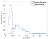 |
Fig. 1. Normalized distribution of spectroscopic redshifts for the lens sample (dashed purple) and photometric redshifts for the source sample (solid blue). |
3. Methods
3.1. Lensing signal
The weak-lensing effect can be characterized by the second derivatives of the lensing potential, ψ, via the Jacobian matrix, 𝒜 (Bartelmann & Schneider 2001):
 (1)
(1)
where the convergence, κ, and lensing shear, γ, in the complex form of γ1 + iγ2, respectively, induce an isotropic size change and elliptical shape distortion on the observed image of the background galaxy. Both of them are related to the second derivatives of the lensing potential, and are thus not independent of each other.
The convergence, specifically, is directly related to the projection of line-of-sight density fluctuations weighted by the lensing efficiency factor, which is expressed as the ratio Σ/Σcrit, with Σ indicating the projected mass density of the lens and Σcrit denoting the critical mass density.
 (2)
(2)
where Ds, Dl, and Dls are the angular diameter distances from the observer to the source, from the observer to the lens, and from the lens to the source, respectively. c denotes the speed of light, and G stands for the Newtonian gravitational constant. As an indicator of lensing efficiency, the critical mass density, Σcrit, for each galaxy cluster was calculated from the redshift distribution of its background sources. On the other hand, the observables for a weak-lensing survey are often the ellipticities of galaxies, which encompass both the intrinsic shape noise of the galaxies and the weak lensing shears γ, or more precisely, the reduced shears g = γ/(1 − κ) (Seitz & Schneider 1997).
The first-year HSC-SSP shear catalog was produced on the coadded i-band images using the re-Gaussianization PSF correction method (Hirata & Seljak 2003; Mandelbaum et al. 2018). The core idea of estimating galaxy shape with this method is to apply a Gaussian profile featuring elliptical isophotes to fit the image, and the components of the distortion are defined as follows:
 (3)
(3)
where b/a is the axis ratio and ϕ is the position angle of the major axis with respect to the equatorial coordinate system (sky coordinates). The ensemble average distortion is then an estimator for the reduced shear, g,
 (4)
(4)
where ℛ is known as the “shear responsivity” and represents the response of the distortion to a small shear (Kaiser et al. 1995; Bernstein & Jarvis 2002; Jarvis et al. 2003).  , where erms is the rms intrinsic distortion per component, typically erms ≃ 0.4.
To carry out comprehensive analyses of our cluster sample, we worked directly on the 2D distortion maps. For all the clusters, we adopted a pixel size of 1 × 1 arcmin2 centered on the observed center (the position of the BCG), and the lensing distortion was measured in a statistical sense, i.e., by averaging the galaxy shapes over an arcminute scale to mitigate the impact of dominant intrinsic shape noise (Oguri et al. 2010). Due to their varying masses and redshifts, different clusters occupy different angular sizes on the sky. Therefore, for each cluster, we gave a first estimate of its mass Mest using the richness-mass relation provided in Rykoff et al. (2012), calculated the cosmic matter density ρm(zcl) at the cluster’s redshift zcl, and derived an estimate of halo radius ![Mathematical equation: $ r_{\mathrm{200m}} = \sqrt[3]{3M_{\mathrm{est}}/{(4\pi\cdot200\rho_{\mathrm{m}}(z_{\mathrm{cl}}))}} $](/articles/aa/full_html/2025/10/aa56332-25/aa56332-25-eq6.gif) , which is defined as the radius within which the mean halo density is 200 times the cosmic matter density ρm(zcl). The total number of pixels on each side could be subsequently obtained by rounding up the angular size θcl = 2 × r200m/DA(zcl) of each cluster in units of arcminute, where DA(zcl) is the angular diameter distance of the cluster. Pixels without any background galaxies were treated as masked and were excluded from the fitting process; these regions naturally appear blank in the shear map (e.g., Fig. 2).
, which is defined as the radius within which the mean halo density is 200 times the cosmic matter density ρm(zcl). The total number of pixels on each side could be subsequently obtained by rounding up the angular size θcl = 2 × r200m/DA(zcl) of each cluster in units of arcminute, where DA(zcl) is the angular diameter distance of the cluster. Pixels without any background galaxies were treated as masked and were excluded from the fitting process; these regions naturally appear blank in the shear map (e.g., Fig. 2).
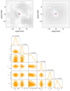 |
Fig. 2. Upper panels: The left panel shows the observed 2D shear map for an illustrative redMaPPer cluster (M ≃ 1014.73 h−1 M⊙), while the right panel displays the corresponding best-fitting shear field predicted by the elliptical NFW model. Each map covers an area of 18′×18′. In both maps, the orientation and length of the sticks within each 1′×′ pixel indicate the local tangential direction and amplitude of the distortion, respectively. For visualization purposes, both shear fields have been smoothed with a Gaussian kernel with a full width at half maximum (FWHM) of ≈2′ (Oguri et al. 2010). The blue dot marks the weak-lensing-derived center, and the red pentagram denotes the observed center. Lower panel: Posterior constraints on structural parameters of the cluster, including the halo concentration, ellipticity, and projected offsets of the mass centroid. The contours represent the 1σ and 2σ confidence levels. |
We followed the approach outlined in Mandelbaum et al. (2018) to compute the weighted shear responsivity factor,  , utilizing the per-object estimates of rms distortion erms, i within each 1 × 1 arcmin2 pixel and the inverse variance weights wi which encode the shape-measurement uncertainty and intrinsic ellipticity dispersion for each galaxy. Specifically, the shear responsivity factor
  in the l-th pixel (its angular position θl) is given by
 (5)
(5)
where i ∈ θl indicates that the summation runs over source galaxies contained within the l-th pixel.
Similarly, the ensemble estimates for calibration biases in the l-th pixel, consisting of both the multiplicative term  and additive term
  , are also derived as a weighted sum of their respective catalog estimates mi and cα, i within the l-th pixel,
 (6)
(6)
 (7)
(7)
where α = 1, 2, denoting the two components of distortion throughout the paper.
Finally, the reduced shear in the l-th pixel is estimated as (Oguri et al. 2010; Mandelbaum et al. 2018)
 (8)
(8)
For the angular scales of interest, the weak-lensing approximation holds, with gα ≈ γα. In subsequent analyses, this approximation was used only when constructing the large-scale-structure covariance (see Eq. (22)); both the model and the data vectors were expressed in terms of the reduced shear gα.
To estimate shape noise per pixel, we randomly rotated source galaxies to eliminate correlated lensing signals and applied the same procedures described above to generate 2D noise distortion maps. For each cluster, we performed 1000 random rotations and consequently obtained 1000 noise distortion maps. The shape noise σγ(θl; α), also comprising two components, was then determined by calculating the standard deviation for each pixel across these 1000 noise distortion maps.
3.2. Cluster mass model
Clusters in the collisionless cold dark matter (CDM) Universe typically exhibit a highly nonspherical structure that was well fitted by a triaxial density profile (e.g., Jing & Suto 2002). We thus constructed an elliptical lens model (Oguri et al. 2010) by incorporating an ellipticity into the isodensity contour, under the assumption that the cluster mass distribution can be described by a single halo component whose radial distribution follows the NFW density profile. Such an elliptical model provided a better description of halos compared to the spherical one (Jing & Suto 2002; Kasun & Evrard 2005; Allgood et al. 2006), since the projection of a triaxial halo along any direction results in elliptical isodensity contours on the convergence map (Oguri et al. 2003; Oguri & Keeton 2004; Heyrovský & Karamazov 2024). Specifically, the following mass model was adopted in the analyses:
 (9)
(9)
 (10)
(10)
 (11)
(11)
 (12)
(12)
where κsph(η) denotes the radial convergence for the spherical NFW model. The halo ellipticity e is defined as e = 1 − b/a, where a and b are the major and minor axis lengths of the isodensity contour. Here we adopted a coordinate system where the coordinate origin is set at the observed center of the cluster (xc, yc) and the position angle θe measured counterclockwise from the positive x axis.
To calculate κsph(η), we adopted the NFW density profile (Navarro et al. 1996, 1997), which is given by
 (13)
(13)
where ρs and rs are the characteristic mass density and scale radius, respectively. It is completely characterized by two parameters, the mass and the halo concentration. The corresponding convergence κsph(η) = (2ρsrs/Σcrit)f(x = η/rs) with (Wright & Brainerd 2000)
![Mathematical equation: $$ \begin{aligned} f(x)=\left\{ \begin{array}{ll} \frac{1}{x^{2}-1}\left[1-\frac{2}{\sqrt{1-x^{2}}} {\text{ arctanh}} \sqrt{\frac{1-x}{1+x}}\right]&x < 1 \\ \frac{1}{3}&x=1 \\ \frac{1}{x^{2}-1}\left[1-\frac{2}{\sqrt{x^{2}-1}} {\text{ arctan}} \sqrt{\frac{x-1}{1+x}}\right]&x>1 \end{array}\right.. \end{aligned} $$](/articles/aa/full_html/2025/10/aa56332-25/aa56332-25-eq20.gif) (14)
(14)
To compute the lensing efficiency, we used the spectroscopic redshift zcl of each cluster and the point-estimate photometric redshifts zp, i of background galaxies to calculate the critical surface mass density Σcrit, i for each source galaxy, according to Eq. (2). The effective critical surface density was then obtained by averaging over all selected background sources within the cluster region using lensing weights wi:
 (15)
(15)
where the summation is over all background galaxies within a θcl × θcl region of the cluster center.
The lensing shear for the elliptical mass model was calculated from κ(x, y) using the relationship between the convergence and the shear (Kaiser & Squires 1993; Seitz & Schneider 1995; Squires & Kaiser 1996). In particular, we used their relation in the Fourier space with
 (16)
(16)
and
 (17)
(17)
The reduced shear was then obtained as g = γ/(1 − κ).
In summary, the elliptical mass model was specified by six parameters:
 (18)
(18)
where M200m is the mass within the halo radius r200m, c200m is the concentration parameter defined as the ratio r200m/rs, e is the halo ellipticity, Δx and Δy represent the offsets along the x and y axes, respectively, from the observed cluster center (xc, yc), and θe is the position angle.
3.3. 2D weak-lensing fitting
To constrain cluster properties, we compared the pixelized 2D distortion field gα(θl), described in Section 3.1, with the reduced shear gαm(θl; p) predicted by the elliptical mass model, where p denotes the parameter set defined in Section 3.2. Specifically, we calculated the χ2 as follows:
![Mathematical equation: $$ \begin{aligned} \begin{aligned} \chi ^2=&\sum _{\alpha ,\beta =1}^{2}\sum _{l,n=1}^{{N_\mathrm{pix} }}\left[g_\alpha (\boldsymbol{\theta }_l)-g_\alpha ^\mathrm{m} (\boldsymbol{\theta }_l;\boldsymbol{p})\right]\left[\boldsymbol{C}^{-1}\right]_{\alpha \beta ,ln}\\&\times \left[g_\beta (\boldsymbol{\theta }_n)-g_\beta ^\mathrm{m} (\boldsymbol{\theta }_n;\boldsymbol{p})\right], \end{aligned} \end{aligned} $$](/articles/aa/full_html/2025/10/aa56332-25/aa56332-25-eq25.gif) (19)
(19)
where the indices α and β run over the two components of reduced shear and the indices l and n denote the position of the pixels. C is the error covariance matrix and C−1 is its inverse. It is expressed as
 (20)
(20)
The term Cshape is dominated by intrinsic shape noise and measurement error. This noise term is expected to be uncorrelated between different pixels; therefore, it is diagonal and is given by
![Mathematical equation: $$ \begin{aligned} \left[{\boldsymbol{C}}^\mathrm{shape}\right]_{\alpha \beta ,ln} = \delta _{\alpha \beta }^K\delta _{ln}^K \sigma ^2_\gamma ({\boldsymbol{\theta }}_l;\alpha ), \end{aligned} $$](/articles/aa/full_html/2025/10/aa56332-25/aa56332-25-eq27.gif) (21)
(21)
where δαβK and δlnK represent the Kronecker delta function, and σγ(θl; α) denotes the shape noise estimated from the noise distortion maps, as described in Section 3.1.
The term Clss presents the covariance due to the large-scale structure, which is given in Hoekstra (2003).
![Mathematical equation: $$ \begin{aligned} \left[{\boldsymbol{C}}^\mathrm{lss}\right]_{\alpha \beta ,ln} = \xi _{\alpha \beta }(|\theta _l - \theta _n|), \end{aligned} $$](/articles/aa/full_html/2025/10/aa56332-25/aa56332-25-eq28.gif) (22)
(22)
the cosmic shear correlation function, ξαβ, is assumed to depend only on the length of the vector connecting the two points θl and θn, due to the statistical isotropy of the Universe. Specifically, the shear correlation functions ξ± are defined through combinations of the two shear components as follows:
 (23)
(23)
 (24)
(24)
![Mathematical equation: $$ \begin{aligned} \xi _{12}(r)&= \cos 2\phi \sin 2\phi \left[\xi _{tt}(r) - \xi _{\times \times }(r)\right], \end{aligned} $$](/articles/aa/full_html/2025/10/aa56332-25/aa56332-25-eq31.gif) (25)
(25)
here, r = |θl − θn|, and ϕ represents the position angle between the coordinate x axis and the vector θl − θn. The functions ξtt and ξ×× correspond to the tangential and cross-component shear correlation functions, respectively (Bartelmann & Schneider 2001). Both of the functions were calculated by the pyccl package6 (Chisari et al. 2019).
We utilized the Markov chain Monte Carlo (MCMC) sampler, emcee package7 (Foreman-Mackey et al. 2013), to explore the χ2 surface, employing a standard Metropolis-Hastings sampling method with a multivariate Gaussian proposal distribution.
Among the six parameters in our model, we imposed a narrow Gaussian prior on the halo mass, with the mean value derived from the mass–richness relation presented in Rykoff et al. (2012),
 (26)
(26)
where A = 1.72 and B = 1.08. The cluster richness, λ, and its measurement uncertainty, σλ, were taken from the redMaPPer catalog, and the corresponding mass uncertainty, σM, was obtained by propagating errors through the above relation. This allowed us to construct a cluster-specific Gaussian prior on halo mass. Our primary interest lay in constraining the structural properties of galaxy clusters, including halo concentration, ellipticity, and the offset between the WL mass centroid and the BCG position. However, uncertainties in halo mass could propagate into these structural parameters and bias their estimation–for example, a massive halo with a downward fluctuation in mass may be incorrectly assigned to a lower mass bin, and vice versa (Du & Fan 2014). Incorporating a mass prior thus helps reduce such biases and improves the robustness of our inference on the connection between halo structure and mass.
For the other five parameters, flat priors in the following ranges were adopted:
-
0 < c200m < 20
-
0 < e < 0.9
-
−θcl/2 < Δx < θcl/2
-
−θcl/2 < Δy < θcl/2
-
0 < θe < π.
The best-fitting model parameters were determined by minimizing the χ2 statistic, while constraints on individual parameters were derived by projecting the MCMC-sampled likelihood distributions onto the parameter space, with marginalization performed over the uncertainties of the other parameters. We calculated the dispersion (standard deviation) of parameters (concentration, ellipticity, and offset) from their posterior distributions of each cluster, and considered the inverse of the square of this dispersion as the weight to calculate the weighted average best-fit parameters in our subsequent analyses.
4. Results
In this section, we presented our main results. The results for individual clusters are described in Section 4.1, with the observed and fitted 2D shear map and the corresponding fitting results for one redMaPPer cluster shown as an example. The concentration-mass relation, the BCG offset distribution, and the cluster ellipticity distribution of our sample are discussed in Sections 4.2, 4.3, and 4.4, respectively.
4.1. Results for individual clusters
For our sample of 299 redMaPPer-selected clusters, we carefully constructed their 2D shear maps using the first-year HSC shear data, following the methodology described in Section 3.1. We then constrained the structural parameters of each cluster by directly fitting these shear maps with elliptical NFW models introduced in Section 3.2 via MCMC (Section 3.3). The analyses primarily focused on the halo concentration, ellipticity, and the distribution of miscentering offsets. The best-fit shear maps predicted by the elliptical NFW model closely reproduce the observed shear patterns, particularly in regions where the tangential shear signal has a high signal-to-noise ratio.
The observed 2D shear map (left) and its corresponding best-fit model (right) for a redMaPPer cluster are presented in the upper panels of Fig. 2 as a representative example. For visualization purposes only, both observed and fitted shear fields have been smoothed with a Gaussian kernel of FWHM ≈ 2′ (Oguri et al. 2010); please note that the unsmoothed shear fields were used in model fitting. In this example, the size of the map is 18′×18′. The orientation and length of the sticks in each 1′×1′ pixel represent the tangential direction and amplitude of the distortion, respectively. The blue dot and the red pentagram represent the center determined by weak lensing and the observed center (position of the BCG), respectively.
The lower panel of Fig. 2 presents posterior constraints on structural parameters, including concentration, ellipticity, and mass centroid offsets of the specific cluster. The contours are for 1σ and 2σ confidence levels. For each parameter, the best-fitting value and the corresponding 68% confidence interval are indicated above the respective one-dimensional marginalized distribution. The projected offsets Δx and Δy are expressed in arcseconds, while the position angle θe is measured in radians, defined counterclockwise from the positive x axis.
4.2. Concentration-mass relation
The concentration parameter characterizes the degree of central mass concentration within a DM halo or cluster. It depends on both the halo’s mass and redshift, and is closely linked to its formation and assembly history. A common observational approach to infer the average concentration is to stack lens–source pairs in bins of similar cluster mass and redshift, then fit the stacked shear profiles with parametric models (Xu et al. 2021).
Here, we measured the concentration of individual dark-matter halos and combined the results from all 299 clusters to statistically constrain the concentration–mass (c–M) relation. In Fig. 3, each gray point represents the best-fitting concentration and mass for a single cluster. We divided the range of log10(M200m) into five equal-width bins. Within each bin, the weighted average of the best-fit concentration and mass was computed, and the corresponding standard deviations are shown as black points with error bars.
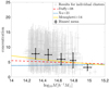 |
Fig. 3. Concentration–mass (c–M) relation. Light gray points represent the best-fitting concentration and mass for individual clusters, while black points show the weighted average values in each mass bin, with error bars indicating the standard deviation. For comparison, the results for strong-lensing selected halos from Meneghetti et al. (2014) are shown by a solid orange line. Weak-lensing-based results from Xu et al. (2021) (upturn model) are plotted as a dashed-dotted blue line, and the power-law model from Duffy et al. (2008) derived from DM-only numerical simulations, is plotted as a dashed red line, respectively. |
To place our results in context, we compared the derived c–M relation with several previous studies, as shown in Fig. 3. The dashed red line corresponds to the power-law model from Duffy et al. (2008), derived from DM-only numerical simulations. The dashed blue line corresponds to the upturn model proposed by Xu et al. (2021), based on weak-lensing measurements using the DECaLS DR8 shear catalog, with a particular emphasis on the high-mass end. We also included results based on strong-lensing selected halos. Meneghetti et al. (2014) estimated the concentrations of CLASH strong-lensing clusters through numerical simulations, using the projected mass distributions to fit NFW profiles, shown as the solid orange line. For a fair comparison, all reference models were evaluated at the mean redshift of our sample, z = 0.339, and we applied appropriate conversions to ensure that their definitions of halo mass and concentration are consistent with those adopted in this work.
As is shown in Fig. 3, our measured c–M relation lies closer to the strong-lensing-selected results of Meneghetti et al. (2014), appears steeper than the power-law relation of Duffy et al. (2008), and shows no indication of an upturn at the high-mass end. This may suggest that our sample selection and fitting methodology are more sensitive to halo concentration at the high-mass end. However, neither the upturn model derived from weak-lensing studies nor the power-law prediction obtained from DM-only numerical simulations can be ruled out within the current level of observational uncertainty.
We further investigated the dependence of concentration in mass-redshift space. In Fig. 4, gray points denote the mass and redshift of individual clusters in our sample. We divided the sample into bins with a redshift interval of 0.15 and a log10(M200m) interval of 0.2. Bins containing fewer than ten clusters were excluded from the analysis. Within each bin, the weighted mean concentration was computed and is shown as diamond symbols. The color of each diamond reflects the average concentration value in that bin, providing a visual representation of the concentration gradient across the mass–redshift plane.
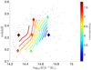 |
Fig. 4. Concentration–mass–redshift (c–M–z) relation. Gray points indicate the positions of individual clusters in the mass–redshift plane. Colored diamonds represent the weighted mean concentration within each bin. Bins containing fewer than ten clusters are excluded from the analysis. Colored contour lines trace surfaces of constant concentration across the plane, and the color bar (labeled “concentration”) gives their numerical values. |
By following the direction of gradient descent along the concentration contours, we find a clear trend: halos with lower redshifts and higher masses exhibit systematically lower concentrations. This trend is consistent with the expectation that more massive clusters at lower redshift are more dynamically relaxed and have had more time to evolve toward equilibrium.
To quantitatively characterize the joint dependence of concentration on both mass and redshift, we adopted a fitting function from Meneghetti et al. (2014) and applied it to the binned, weighted-mean concentrations in our sample:
 (27)
(27)
here, zmean = 0.339 and Mmean = 3.058 × 10¹⁴ h−1 M⊙ represent the mean redshift and the mean mass of the sample, respectively. The best-fitting parameters and their associated uncertainties corresponding to the 68% confidence interval are summarized in Table 1.
Best-fitting parameters for the concentration–mass–redshift (c–M–z) relation derived from our cluster sample.
Due to limitations in sample size and observational conditions, the precision of our quantitative characterization of the c–M–z relation is somewhat constrained. Nevertheless, the overall trend reveals a negative correlation of concentration with both halo mass and redshift.
4.3. Offset between lensing center and BCG
In observational studies, halo centers are typically identified with either the position of a massive galaxy (e.g., the BCG) or the peak of the hot gas distribution. This is because the lensing center of mass, dominated by invisible DM, is not directly observable. Miscentering between the true mass center and these observational tracers is a significant source of systematic uncertainty in stacked weak-lensing analyses (Johnston et al. 2007; Sommer et al. 2025). Correcting for this effect not only improves the accuracy of mass measurements but also enhances our understanding of the nature of DM (Harvey et al. 2015).
Weak lensing provides a unique and independent means of locating the lensing center of a DM halo, as it directly probes the projected gravitational potential and is sensitive to the full matter distribution. It thus offers a complementary perspective to optical indicators (e.g., BCGs) and thermal signals from the Sunyaev–Zel’dovich (SZ) effect (Ding et al. 2025).
In modeling the miscentering effect in weak lensing analyses, a 2D Gaussian distribution is widely adopted as a realistic representation of offset distributions. Following the approach of Oguri et al. (2018), we modeled the BCG offset distribution using a two-component 2D Gaussian function, as shown in Fig. 5, which enables a flexible description of both well-centered and miscentered populations:
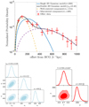 |
Fig. 5. Upper panel: Probability distribution function (PDF) of the projected offset between the BCG position and the weak-lensing-determined halo center. Red data points show the observed BCG offsets in our sample, with error bars estimated via 1000 bootstrap resamplings. The solid blue and black lines represent the best-fitting single- and two-component 2D Gaussian models, respectively. The dashed purple and orange lines correspond to the well-centered and miscentered components of the two-component model. All offset scale parameters, including σ, σ1, and σ2, are expressed in units of h−1 kpc. Lower panels: Fitting results for the two-component (left) and single-component (right) 2D Gaussian models. Contours indicate 1σ and 2σ confidence levels, with best-fitting values and 68% confidence intervals shown above each 1D marginalized distribution. |
 (28)
(28)
Here, Roff denotes the projected separation between the weak-lensing-determined halo center and the BCG position. The parameter fcen represents the fraction of well-centered clusters, while σ1 and σ2 describe the characteristic offset scales of the well-centered and miscentered components, respectively. Parameter uncertainties were estimated via 1000 bootstrap resamplings. The reduced χ2 values for the single- and two-component models are 8.58 and 0.87, respectively, confirming the superior fit of the two-component model.
The upper panel of Fig. 5 displays the weighted distribution of BCG–WL centroid offsets. The solid blue line represents a single 2D Gaussian fit with a characteristic scale of  kpc, which evidently fails to capture the bimodality. The best-fitting parameters for the two-component model are fcen = 0.43 ± 0.05,
  kpc for the well-centered population, and
  kpc for the miscentered population.
We notice that, for a few clusters, the inferred offsets were close to the edge of the default fitting range [ − θcl/2, θcl/2]. To test the robustness of our offset measurements and to evaluate whether this boundary could bias the results, we repeated the fitting for these clusters using an expanded data range of [ − θcl, θcl], while keeping the offset prior unchanged. The resulting parameter constraints remain consistent within uncertainties, confirming the stability and reliability of the fitted offset distribution.
We further divided the sample into high- and low-mass subsamples based on the median halo mass. Offsets in the low-mass bin exhibit larger values of σ1 and σ2, suggesting that lower-mass halos in our sample may be more affected by surrounding large-scale structure and projection effects, leading to greater displacements between the WL center and the BCG.
Similarly, when dividing the sample into high- and low-redshift bins, we find that the low-redshift clusters tend to have higher values of fcen and smaller offset scales. This trend is consistent with the expectation that halos become more dynamically relaxed over time, resulting in better alignment between the mass centroid and the BCG. These comparisons are illustrated in Fig. 6, which shows the projected offset distributions and the corresponding best-fit parameters for different redshift and mass bins.
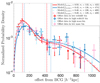 |
Fig. 6. Probability distribution functions (PDFs) of the projected offsets between the BCG and the weak-lensing-determined halo center for different redshift and mass bins. All error bars are estimated from 1000 bootstrap resamplings. Red and blue points represent the low- and high-redshift subsamples, respectively, with solid lines showing the best-fitting two-component 2D Gaussian models. Corresponding vertical lines indicate the values of σ1 and σ2. Pink and light blue points show the low- and high-mass subsamples, respectively, with dashed lines and vertical markers indicating the best fits and offset scales. |
We note that the miscentering parameters inferred from our BCG-WL offsets differ from those reported in previous studies. For example, the fcen value shown in Fig. 5 is lower than that obtained by Oguri et al. (2018), while our offset scales (σ1 and σ2) are larger than their reported values of 46 ± 9 h−1 kpc and 260 ± 40 h−1 kpc, respectively. This discrepancy may arise from differences in center definitions and sample selection. Notably, Oguri et al. (2018) measured the offsets between BCGs and X-ray centers of clusters, with the X-ray temperatures estimated using a mass–temperature relation based on M500, which corresponds to more compact regions than the M200m used in our analysis. Motivated by the relatively large WL–BCG offsets, we further investigated whether this trend reflects genuine physical differences between weak-lensing and baryon-based tracers. As a first step, we compared the optical centers from redMaPPer with those from two other optical catalogs – HSC S19A (Aihara et al. 2022) and WH2022 (Wen & Han 2022). For each HSC or WH2022 cluster, we identified the nearest redMaPPer counterpart using the match_to_catalog_sky method in astropy’s SkyCoord class (Astropy Collaboration 2022), with a maximum separation of 1 arcmin. We find that more than 85% of the matched clusters have projected offsets smaller than 100 kpc, indicating that the optical-optical center differences are negligible.
We then compared the redMaPPer optical centers with those determined from SZ observations (ACT DR5; Naess et al. 2020) and X-ray data (Ghirardini et al. 2024), computing the projected physical offsets using redMaPPer photometric redshifts. In this calculation, we adopted a maximum offset threshold corresponding to a typical cluster size (∼1 h−1 Mpc) to exclude spurious large separations. The resulting offset distributions and their best-fitting two-component models are shown in Fig. 7, along with several results from the literature (Ding et al. 2025; Oguri et al. 2018) for comparison. Although the exact values of fcen, σ1, and σ2 vary among studies, the overall shapes of the offset distributions are broadly consistent.
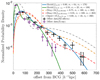 |
Fig. 7. Probability distribution functions (PDFs) of the projected offsets between the BCG position and the SZ- or X-ray-determined cluster centers. Black and purple data points represent the offsets between the redMaPPer optical centers and the SZ (ACT DR5) or X-ray cluster centers, respectively. The solid blue and green lines show the best-fitting two-component 2D Gaussian models for the SZ and X-ray cases. The dashed orange and red lines show results from Ding et al. (2025): the orange line corresponds to all 186 optical–SZ cross-matched clusters, while the red line excludes clusters affected by astrophysical effects (e.g., ongoing mergers) or systematic biases in the HSC data and cluster-finding algorithm. The dashed gray line shows the X-ray–optical offset distribution from Oguri et al. (2018), based on HSC Wide S16A clusters. All offsets are shown in physical units of h−1 kpc. |
Therefore, the offsets involving SZ or X-ray centers are significantly smaller than those based on weak-lensing-determined centers. This suggests that weak lensing is identifying a different characteristic center–one that traces the projected gravitational potential and is influenced by the full matter distribution along the line of sight weighted by lensing efficiency.
Unlike X-ray or SZ signals, which trace the distribution of hot baryonic gas through electron density and temperature, weak lensing directly probes the total mass, including both baryonic and DM, and is independent of the dynamical state of the cluster. Consequently, in unrelaxed systems or in clusters embedded in complex environments with substantial line-of-sight structures, weak-lensing-derived centers may appear significantly offset from the baryon-based tracers. These intrinsic differences in physical sensitivity and projection response among tracers likely contribute to the broader offset distributions observed in WL-based analyses.
For clusters with the largest centroid offsets, the projected distributions of member galaxies are found to be frequently bimodal, suggesting ongoing mergers or significant dynamical disturbances; however, given the current data quality and the unknown dynamical information of the clusters, we refrain from definitive classification and defer a more detailed analysis to future work.
4.4. Distribution of halo ellipticities
Ellipticity is a key parameter used to characterize the projected shape of DM halos along the line of sight, and its importance in understanding halo structure is well established. Although the spherically symmetric NFW model successfully reproduces the spherical average of the halo density profile, both N-body simulations (Jing & Suto 2002) and observations (Oguri et al. 2010; Liu et al. 2025) consistently show that halos are intrinsically nonspherical.
Moreover, halo shape provides insights into the nature of DM. For instance, halos in self-interacting dark matter (SIDM) models are predicted to be more spherical than those in CDM scenarios, as particle self-interactions tend to isotropize the DM distribution (Gonzalez et al. 2024).
In our analysis, we performed an individual shear map fitting for each cluster to estimate its own ellipticity, and then combined the resulting values to construct the overall probability distribution, as shown in Fig. 8. This approach captures the intrinsic variation in halo shapes across the sample. Errors were estimated using 1000 bootstrap resamplings. The measured ellipticity for the full sample is e = 0.530 ± 0.168, and the mean ellipticity is ⟨e⟩ = 0.505 ± 0.007, which is in good agreement with predictions from N-body simulations (Jing & Suto 2002) and previous observational results (Liu et al. 2025).
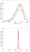 |
Fig. 8. Upper panel: Probability distribution function (PDF) of the ellipticity values derived from individual shear map fittings of each cluster. Blue points represent the observed distribution, with error bars estimated from 1000 bootstrap resamplings. The red curve shows a Gaussian fit to the distribution, centered at e = 0.530 ± 0.168. For comparison, the dashed black line represents the ellipticity distribution reported by Liu et al. (2025), converted to match our ellipticity definition. Lower panel: PDF of the sample-averaged ellipticity, ⟨e⟩, computed from the full cluster ensemble. The red curve shows a Gaussian fit centered at ⟨e⟩ = 0.505 ± 0.007. |
In Table 2, we divided the sample into four subsets in the mass–redshift plane based on the mean halo mass and mean redshift. Specifically, clusters are grouped into quadrants: (1) low mass & low redshift, (2) low mass & high redshift, (3) high mass & low redshift, and (4) high mass & high redshift. We computed the average ellipticity in each bin. The results show that halos with higher mass and lower redshift tend to exhibit slightly lower ellipticities, implying that they appear more spherical along the line of sight. This trend contrasts with predictions from DM-only cosmological simulations (Jing & Suto 2002; Lau et al. 2021), which include only gravitational interactions. These simulations typically find that more massive and lower-redshift halos are slightly more elliptical due to persistent anisotropic mass accretion from the surrounding cosmic web. Interestingly, our findings align more closely with the trend for halo masses larger than 1013.5 h−1 M⊙ in the hydrodynamical IllustrisTNG simulation (Liu et al. 2025), which incorporates baryonic physics. In this context, more massive halos are expected to assemble earlier and more rapidly, reducing subsequent interactions with their large-scale environments and thus evolving into more isotropic and spherical configurations.
The ellipticity distribution in different mass–redshift bins.
5. Conclusion and discussion
In this paper, we have analyzed 299 individual redMaPPer-selected clusters by constructing their 2D shear maps from the HSC first-year shear catalog with high data quality. We statistically investigated key halo properties, including concentration, ellipticity, and the BCG offset. To mitigate the impact of intrinsic mass uncertainties on the statistical concentration–mass(c–M) relation, we adopted a mass–richness prior from Rykoff et al. (2012) in our fitting procedure. Furthermore, we used the inverse of the posterior variance of each fitted parameter as the statistical weight when computing weighted average values. Our main conclusions are as follows:
-
We find that halo concentration decreases with increasing mass in our sample. The derived c–M relation is steeper than those obtained from weak lensing analyses but more consistent with trends seen in strong-lensing-selected cluster studies. This may reflect that our sample selection and fitting method are more sensitive to halo concentration at the high-mass end. In the mass–redshift plane, we observe that halos with lower redshift and higher mass tend to have lower concentrations.
-
The distribution of offsets between the observed optical center and the weak-lensing-determined center is well described by a two-component 2D Gaussian model, as defined in Eq. (28). The characteristic offset scales are
 kpc and
  kpc, corresponding to the well-centered and miscentered populations, respectively. The fraction of well-centered clusters is measured as fcen = 0.43 ± 0.05. We find that halos in the lower mass bin tend to exhibit larger offsets, possibly due to their greater susceptibility to perturbations from surrounding large-scale structures and enhanced lensing projection effects. In comparison, lower-redshift clusters exhibit smaller offsets and higher centering fractions, consistent with the expectation that clusters become more relaxed over cosmic time. The weak-lensing-based offsets are systematically larger than those involving X-ray or SZ-defined centers (Oguri et al. 2018; Ding et al. 2025), likely reflecting differences in tracer sensitivity and center definitions. In particular, weak lensing probes the total projected mass distribution – including DM – while X-ray and SZ observations trace the hot baryonic gas, which is more tightly correlated with the optical BCG position. These intrinsic physical differences among tracers naturally lead to broader offset distributions in WL-based measurements. Our results demonstrate that modeling miscentering with a flexible two-component model significantly improves the reliability of halo property inference. This is crucial for reducing systematics in GGL analyses and for ensuring the robustness of high-precision cosmological probes, such as cluster abundance studies (Ghirardini et al. 2024) and three-by-two-point (3 × 2 pt) analyses (Heymans et al. 2021; Li et al. 2023b; DES Collaboration 2025), where even small biases in halo centering can impact cosmological parameter constraints. A more detailed treatment of these effects will be presented in a forthcoming paper.
 -
The ellipticity distribution derived from individual cluster fittings has a mean value of e = 0.530 ± 0.168, and the sample-averaged ellipticity is ⟨e⟩ = 0.505 ± 0.007. In the mass–redshift plane, halos with higher mass and lower redshift appear more spherical, exhibiting slightly lower average ellipticities. This trend is opposite to predictions from dark-matter-only N-body simulations but is more closely consistent with the trend for halo masses larger than 1013.5 h−1 M⊙ from the IllustrisTNG simulations (Liu et al. 2025) that include baryonic effects. In those models, baryonic cooling contracts matter toward the center, increasing halo roundness (Lau et al. 2012), while isotropic momentum redistribution from merger events also promotes spherical shapes. A similar effect is observed in SIDM models, where particle collisions isotropize the halo structure (Gonzalez et al. 2024). Although our current measurements cannot distinguish between these two physical mechanisms, the results offer meaningful constraints on the nature of DM.
Overall, our results demonstrate that 2D weak-lensing analysis is a powerful tool for investigating the structural properties of individual galaxy clusters, and it holds significant potential for improving the treatment of systematic uncertainties in traditional stacking methods. Future wide-field surveys, such as the Vera C. Rubin Observatory, the Euclid mission, and CSST, will deliver larger samples of clusters and background galaxies, enabling more precise constraints on halo properties and offering new opportunities to probe the fundamental nature of DM.
Acknowledgments
This research is supported by National Key R&D Program of China No. 2022YFF0503403. X.K.L. acknowledges the support from NSFC grant No. 12173033, the grants from the China Manned Space Projects with No. CMS-CSST-2021-B01, the “Yunnan Key Laboratory of Survey Science” with project No. 202449CE340002 and a “Yunnan Provincial Top Team Projects” with project No. 202305AT350002. H.Y.S. acknowledges the support from the Ministry of Science and Technology of China (grant No. 2020SKA0110100), Key Research Program of Frontier Sciences, CAS, Grant No. ZDBS-LY-7013 and Program of Shanghai Academic/Technology Research Leader. Z.H.F. acknowledges the support from NSFC grant No. 11933002, and the grant from the China Manned Space Projects with No. CMS-CSST-2021-A01. We also acknowledge the support from the science research grants from the China Manned Space Project with No. CMS-CSST-2025-A03 and CMS-CSST-2025-A05. Part of the computations in this study were carried out on the servers of the SWIFAR Cosmology Group and the Yunnan University Astronomy Supercomputer. The Hyper Suprime-Cam (HSC) collaboration includes the astronomical communities of Japan and Taiwan, and Princeton University. The HSC instrumentation and software were developed by the National Astronomical Observatory of Japan (NAOJ), the Kavli Institute for the Physics and Mathematics of the Universe (Kavli IPMU), the University of Tokyo, the High Energy Accelerator Research Organization (KEK), the Academia Sinica Institute for Astronomy and Astrophysics in Taiwan (ASIAA), and Princeton University. Funding was contributed by the FIRST program from the Japanese Cabinet Office, the Ministry of Education, Culture, Sports, Science and Technology (MEXT), the Japan Society for the Promotion of Science (JSPS), Japan Science and Technology Agency (JST), the Toray Science Foundation, NAOJ, Kavli IPMU, KEK, ASIAA, and Princeton University. This paper makes use of software developed for Vera C. Rubin Observatory. We thank the Rubin Observatory for making their code available as free software at http://pipelines.lsst.io. This paper is based on data collected at the Subaru Telescope and retrieved from the HSC data archive system, which is operated by the Subaru Telescope and Astronomy Data Center (ADC) at NAOJ. Data analysis was in part carried out with the cooperation of Center for Computational Astrophysics (CfCA), NAOJ. We are honored and grateful for the opportunity of observing the Universe from Maunakea, which has the cultural, historical and natural significance in Hawaii. The Pan-STARRS1 Surveys (PS1) and the PS1 public science archive have been made possible through contributions by the Institute for Astronomy, the University of Hawaii, the Pan-STARRS Project Office, the Max Planck Society and its participating institutes, the Max Planck Institute for Astronomy, Heidelberg, and the Max Planck Institute for Extraterrestrial Physics, Garching, The Johns Hopkins University, Durham University, the University of Edinburgh, the Queen’s University Belfast, the Harvard-Smithsonian Center for Astrophysics, the Las Cumbres Observatory Global Telescope Network Incorporated, the National Central University of Taiwan, the Space Telescope Science Institute, the National Aeronautics and Space Administration under grant No. NNX08AR22G issued through the Planetary Science Division of the NASA Science Mission Directorate, the National Science Foundation grant No. AST-1238877, the University of Maryland, Eotvos Lorand University (ELTE), the Los Alamos National Laboratory, and the Gordon and Betty Moore Foundation.
References
- Aihara, H., Allende Prieto, C., An, D., et al. 2011, ApJS, 193, 29 [NASA ADS] [CrossRef] [Google Scholar]
- Aihara, H., Armstrong, R., Bickerton, S., et al. 2018, PASJ, 70, S8 [NASA ADS] [Google Scholar]
- Aihara, H., AlSayyad, Y., Ando, M., et al. 2022, PASJ, 74, 247 [NASA ADS] [CrossRef] [Google Scholar]
- Allgood, B., Flores, R. A., Primack, J. R., et al. 2006, MNRAS, 367, 1781 [NASA ADS] [CrossRef] [Google Scholar]
- Astropy Collaboration (Price-Whelan, A. M., et al.) 2022, ApJ, 935, 167 [NASA ADS] [CrossRef] [Google Scholar]
- Bartelmann, M., & Schneider, P. 2001, Phys. Rep., 340, 291 [Google Scholar]
- Bernstein, G. M., & Jarvis, M. 2002, AJ, 123, 583 [NASA ADS] [CrossRef] [Google Scholar]
- Brainerd, T. G. 2005, ApJ, 628, L101 [Google Scholar]
- Bullock, J. S., Kolatt, T. S., Sigad, Y., et al. 2001, MNRAS, 321, 559 [Google Scholar]
- Cacciato, M., van den Bosch, F. C., More, S., et al. 2009, MNRAS, 394, 929 [NASA ADS] [CrossRef] [Google Scholar]
- Carlstrom, J. E., Holder, G. P., & Reese, E. D. 2002, ARA&A, 40, 643 [Google Scholar]
- Child, H. L., Habib, S., Heitmann, K., et al. 2018, ApJ, 859, 55 [NASA ADS] [CrossRef] [Google Scholar]
- Chisari, N. E., Alonso, D., Krause, E., et al. 2019, ApJS, 242, 2 [Google Scholar]
- Cui, W., Knebe, A., Yepes, G., et al. 2018, MNRAS, 480, 2898 [Google Scholar]
- Cypriano, E. S., Sodré, L., Kneib, J.-P., & Campusano, L. E. 2004, ApJ, 613, 95 [Google Scholar]
- Dark Energy Survey Collaboration (Abbott, T., et al.) 2016, MNRAS, 460, 1270 [Google Scholar]
- de Jong, J. T. A., Verdoes Kleijn, G. A., Kuijken, K. H., & Valentijn, E. A. 2013, Exp. Astron., 35, 25 [Google Scholar]
- Deb, S., Goldberg, D. M., Heymans, C., & Morandi, A. 2010, ApJ, 721, 124 [Google Scholar]
- DES Collaboration (Abbott, T. M. C., et al.) 2025, ArXiv e-prints [arXiv:2503.13632] [Google Scholar]
- Diego, J. M., Congedo, G., Gavazzi, R., et al. 2025, A&A, submitted [arXiv:2507.08545] [Google Scholar]
- Ding, J., Dalal, R., Sunayama, T., et al. 2025, MNRAS, 536, 572 [Google Scholar]
- Du, W., & Fan, Z. 2014, ApJ, 785, 57 [Google Scholar]
- Duffy, A. R., Schaye, J., Kay, S. T., & Dalla Vecchia, C. 2008, MNRAS, 390, L64 [Google Scholar]
- Foreman-Mackey, D., Hogg, D. W., Lang, D., & Goodman, J. 2013, PASP, 125, 306 [Google Scholar]
- Fu, L.-P., & Fan, Z.-H. 2014, RAA, 14, 1061 [NASA ADS] [Google Scholar]
- George, M. R., Leauthaud, A., Bundy, K., et al. 2012, ApJ, 757, 2 [NASA ADS] [CrossRef] [Google Scholar]
- Ghirardini, V., Bulbul, E., Artis, E., et al. 2024, A&A, 689, A298 [NASA ADS] [CrossRef] [EDP Sciences] [Google Scholar]
- Gonzalez, E. J., Makler, M., García Lambas, D., et al. 2021, MNRAS, 501, 5239 [CrossRef] [Google Scholar]
- Gonzalez, E. J., Rodríguez-Medrano, A., Pereyra, L., & García Lambas, D. 2024, MNRAS, 528, 3075 [NASA ADS] [CrossRef] [Google Scholar]
- Harvey, D., Massey, R., Kitching, T., Taylor, A., & Tittley, E. 2015, Science, 347, 1462 [Google Scholar]
- Heymans, C., Van Waerbeke, L., Miller, L., et al. 2012, MNRAS, 427, 146 [Google Scholar]
- Heymans, C., Tröster, T., Asgari, M., et al. 2021, A&A, 646, A140 [NASA ADS] [CrossRef] [EDP Sciences] [Google Scholar]
- Heyrovský, D., & Karamazov, M. 2024, A&A, 690, A19 [NASA ADS] [CrossRef] [EDP Sciences] [Google Scholar]
- Hirata, C., & Seljak, U. 2003, MNRAS, 343, 459 [Google Scholar]
- Hoekstra, H. 2003, MNRAS, 339, 1155 [NASA ADS] [CrossRef] [Google Scholar]
- Hoekstra, H., & Jain, B. 2008, Annu. Rev. Nucl. Part. Sci., 58, 99 [NASA ADS] [CrossRef] [Google Scholar]
- Hsieh, B. C., & Yee, H. K. C. 2014, ApJ, 792, 102 [Google Scholar]
- Jarvis, M., Bernstein, G. M., Fischer, P., et al. 2003, AJ, 125, 1014 [NASA ADS] [CrossRef] [Google Scholar]
- Jenkins, A., Frenk, C. S., White, S. D. M., et al. 2001, MNRAS, 321, 372 [Google Scholar]
- Jing, Y. P., & Suto, Y. 2002, ApJ, 574, 538 [Google Scholar]
- Johnston, D. E., Sheldon, E. S., Wechsler, R. H., et al. 2007, ArXiv e-prints [arXiv:0709.1159] [Google Scholar]
- Kaiser, N., & Squires, G. 1993, ApJ, 404, 441 [Google Scholar]
- Kaiser, N., Squires, G., & Broadhurst, T. 1995, ApJ, 449, 460 [Google Scholar]
- Kasun, S. F., & Evrard, A. E. 2005, ApJ, 629, 781 [NASA ADS] [CrossRef] [Google Scholar]
- Kilbinger, M. 2015, Rep. Progr. Phys., 78, 086901 [Google Scholar]
- Lau, E. T., Nagai, D., Kravtsov, A. V., Vikhlinin, A., & Zentner, A. R. 2012, ApJ, 755, 116 [NASA ADS] [CrossRef] [Google Scholar]
- Lau, E. T., Hearin, A. P., Nagai, D., & Cappelluti, N. 2021, MNRAS, 500, 1029 [Google Scholar]
- Laureijs, R., Amiaux, J., Arduini, S., et al. 2011, ArXiv e-prints [arXiv:1110.3193] [Google Scholar]
- Li, X., Miyatake, H., Luo, W., et al. 2022, PASJ, 74, 421 [NASA ADS] [CrossRef] [Google Scholar]
- Li, Z., Liu, X., & Fan, Z. 2023a, MNRAS, 520, 6382 [Google Scholar]
- Li, X., Zhang, T., Sugiyama, S., et al. 2023b, Phys. Rev. D, 108, 123518 [CrossRef] [Google Scholar]
- Li, Q., Kilbinger, M., Luo, W., et al. 2024, ApJ, 969, L25 [Google Scholar]
- Liu, Z., Zhang, J., Liu, C., & Li, H. 2025, ApJ, 979, 200 [Google Scholar]
- Ludlow, A. D., Bose, S., Angulo, R. E., et al. 2016, MNRAS, 460, 1214 [Google Scholar]
- Luo, R., Fu, L., Luo, W., et al. 2022, A&A, 668, A12 [Google Scholar]
- Luo, W., Silverman, J. D., More, S., et al. 2024, ApJ, 977, 59 [Google Scholar]
- Macciò, A. V., Dutton, A. A., van den Bosch, F. C., et al. 2007, MNRAS, 378, 55 [Google Scholar]
- Mandelbaum, R., Hirata, C. M., Seljak, U., et al. 2005, MNRAS, 361, 1287 [Google Scholar]
- Mandelbaum, R., Seljak, U., Kauffmann, G., Hirata, C. M., & Brinkmann, J. 2006a, MNRAS, 368, 715 [NASA ADS] [CrossRef] [Google Scholar]
- Mandelbaum, R., Seljak, U., Cool, R. J., et al. 2006b, MNRAS, 372, 758 [NASA ADS] [CrossRef] [Google Scholar]
- Mandelbaum, R., Seljak, U., & Hirata, C. M. 2008, JCAP, 2008, 006 [Google Scholar]
- Mandelbaum, R., Slosar, A., Baldauf, T., et al. 2013, MNRAS, 432, 1544 [NASA ADS] [CrossRef] [Google Scholar]
- Mandelbaum, R., Miyatake, H., Hamana, T., et al. 2018, PASJ, 70, S25 [Google Scholar]
- Meneghetti, M., Rasia, E., Vega, J., et al. 2014, ApJ, 797, 34 [Google Scholar]
- Naess, S., Aiola, S., Austermann, J. E., et al. 2020, JCAP, 2020, 046 [Google Scholar]
- Nagai, D., & Kravtsov, A. V. 2005, ApJ, 618, 557 [Google Scholar]
- Nagai, D., Vikhlinin, A., & Kravtsov, A. V. 2007, ApJ, 655, 98 [Google Scholar]
- Navarro, J. F., Frenk, C. S., & White, S. D. M. 1996, ApJ, 462, 563 [Google Scholar]
- Navarro, J. F., Frenk, C. S., & White, S. D. M. 1997, ApJ, 490, 493 [Google Scholar]
- Oguri, M., & Keeton, C. R. 2004, ApJ, 610, 663 [Google Scholar]
- Oguri, M., Lee, J., & Suto, Y. 2003, ApJ, 599, 7 [NASA ADS] [CrossRef] [Google Scholar]
- Oguri, M., Takada, M., Okabe, N., & Smith, G. P. 2010, MNRAS, 405, 2215 [NASA ADS] [Google Scholar]
- Oguri, M., Lin, Y.-T., Lin, S.-C., et al. 2018, PASJ, 70, S20 [NASA ADS] [Google Scholar]
- Osato, K., Nishimichi, T., Oguri, M., Takada, M., & Okumura, T. 2018, MNRAS, 477, 2141 [NASA ADS] [CrossRef] [Google Scholar]
- Peebles, P. J. E. 1980, The Large-Scale Structure of the Universe (Princeton: Princeton University Press) [Google Scholar]
- Peter, A. H. G., Rocha, M., Bullock, J. S., & Kaplinghat, M. 2013, MNRAS, 430, 105 [Google Scholar]
- Planck Collaboration XXIV. 2016, A&A, 594, A24 [NASA ADS] [CrossRef] [EDP Sciences] [Google Scholar]
- Planck Collaboration VI. 2020, A&A, 641, A6 [NASA ADS] [CrossRef] [EDP Sciences] [Google Scholar]
- Press, W. H., & Schechter, P. 1974, ApJ, 187, 425 [Google Scholar]
- Rykoff, E. S., Koester, B. P., Rozo, E., et al. 2012, ApJ, 746, 178 [NASA ADS] [CrossRef] [Google Scholar]
- Rykoff, E. S., Rozo, E., Busha, M. T., et al. 2014, ApJ, 785, 104 [Google Scholar]
- Rykoff, E. S., Rozo, E., Hollowood, D., et al. 2016, ApJS, 224, 1 [NASA ADS] [CrossRef] [Google Scholar]
- Schrabback, T., Congedo, G., Gavazzi, R., et al. 2025, A&A, submitted [arXiv:2507.07629] [Google Scholar]
- Seitz, C., & Schneider, P. 1995, A&A, 297, 287 [NASA ADS] [Google Scholar]
- Seitz, C., & Schneider, P. 1997, A&A, 318, 687 [NASA ADS] [Google Scholar]
- Shan, H., Kneib, J.-P., Li, R., et al. 2017, ApJ, 840, 104 [NASA ADS] [CrossRef] [Google Scholar]
- Shan, H., Liu, X., Hildebrandt, H., et al. 2018, MNRAS, 474, 1116 [Google Scholar]
- Sheth, R. K., & Tormen, G. 1999, MNRAS, 308, 119 [Google Scholar]
- Sohn, J., Geller, M. J., Diaferio, A., & Rines, K. J. 2020, ApJ, 891, 129 [NASA ADS] [CrossRef] [Google Scholar]
- Sommer, M. W., Schrabback, T., & Grandis, S. 2025, MNRAS, 538, L50 [Google Scholar]
- Squires, G., & Kaiser, N. 1996, ApJ, 473, 65 [Google Scholar]
- Tanaka, M., Coupon, J., Hsieh, B.-C., et al. 2018, PASJ, 70, S9 [Google Scholar]
- Tinker, J., Kravtsov, A. V., Klypin, A., et al. 2008, ApJ, 688, 709 [Google Scholar]
- Vale, C., & White, M. 2006, New Astron., 11, 207 [Google Scholar]
- Wang, C., Li, R., Shan, H., et al. 2024, MNRAS, 528, 2728 [NASA ADS] [CrossRef] [Google Scholar]
- Watson, W. A., Iliev, I. T., D’Aloisio, A., et al. 2013, MNRAS, 433, 1230 [Google Scholar]
- Wen, Z. L., & Han, J. L. 2022, MNRAS, 513, 3946 [NASA ADS] [CrossRef] [Google Scholar]
- Wright, C. O., & Brainerd, T. G. 2000, ApJ, 534, 34 [Google Scholar]
- Xu, W., Shan, H., Li, R., et al. 2021, ApJ, 922, 162 [Google Scholar]
- Zel’dovich, Y. B. 1970, A&A, 5, 84 [NASA ADS] [Google Scholar]
- Zu, Y., & Mandelbaum, R. 2015, MNRAS, 454, 1161 [Google Scholar]
All Tables
Best-fitting parameters for the concentration–mass–redshift (c–M–z) relation derived from our cluster sample.
All Figures
|
Fig. 1. Normalized distribution of spectroscopic redshifts for the lens sample (dashed purple) and photometric redshifts for the source sample (solid blue). |
| In the text | |
|
Fig. 2. Upper panels: The left panel shows the observed 2D shear map for an illustrative redMaPPer cluster (M ≃ 1014.73 h−1 M⊙), while the right panel displays the corresponding best-fitting shear field predicted by the elliptical NFW model. Each map covers an area of 18′×18′. In both maps, the orientation and length of the sticks within each 1′×′ pixel indicate the local tangential direction and amplitude of the distortion, respectively. For visualization purposes, both shear fields have been smoothed with a Gaussian kernel with a full width at half maximum (FWHM) of ≈2′ (Oguri et al. 2010). The blue dot marks the weak-lensing-derived center, and the red pentagram denotes the observed center. Lower panel: Posterior constraints on structural parameters of the cluster, including the halo concentration, ellipticity, and projected offsets of the mass centroid. The contours represent the 1σ and 2σ confidence levels. |
| In the text | |
|
Fig. 3. Concentration–mass (c–M) relation. Light gray points represent the best-fitting concentration and mass for individual clusters, while black points show the weighted average values in each mass bin, with error bars indicating the standard deviation. For comparison, the results for strong-lensing selected halos from Meneghetti et al. (2014) are shown by a solid orange line. Weak-lensing-based results from Xu et al. (2021) (upturn model) are plotted as a dashed-dotted blue line, and the power-law model from Duffy et al. (2008) derived from DM-only numerical simulations, is plotted as a dashed red line, respectively. |
| In the text | |
|
Fig. 4. Concentration–mass–redshift (c–M–z) relation. Gray points indicate the positions of individual clusters in the mass–redshift plane. Colored diamonds represent the weighted mean concentration within each bin. Bins containing fewer than ten clusters are excluded from the analysis. Colored contour lines trace surfaces of constant concentration across the plane, and the color bar (labeled “concentration”) gives their numerical values. |
| In the text | |
|
Fig. 5. Upper panel: Probability distribution function (PDF) of the projected offset between the BCG position and the weak-lensing-determined halo center. Red data points show the observed BCG offsets in our sample, with error bars estimated via 1000 bootstrap resamplings. The solid blue and black lines represent the best-fitting single- and two-component 2D Gaussian models, respectively. The dashed purple and orange lines correspond to the well-centered and miscentered components of the two-component model. All offset scale parameters, including σ, σ1, and σ2, are expressed in units of h−1 kpc. Lower panels: Fitting results for the two-component (left) and single-component (right) 2D Gaussian models. Contours indicate 1σ and 2σ confidence levels, with best-fitting values and 68% confidence intervals shown above each 1D marginalized distribution. |
| In the text | |
|
Fig. 6. Probability distribution functions (PDFs) of the projected offsets between the BCG and the weak-lensing-determined halo center for different redshift and mass bins. All error bars are estimated from 1000 bootstrap resamplings. Red and blue points represent the low- and high-redshift subsamples, respectively, with solid lines showing the best-fitting two-component 2D Gaussian models. Corresponding vertical lines indicate the values of σ1 and σ2. Pink and light blue points show the low- and high-mass subsamples, respectively, with dashed lines and vertical markers indicating the best fits and offset scales. |
| In the text | |
|
Fig. 7. Probability distribution functions (PDFs) of the projected offsets between the BCG position and the SZ- or X-ray-determined cluster centers. Black and purple data points represent the offsets between the redMaPPer optical centers and the SZ (ACT DR5) or X-ray cluster centers, respectively. The solid blue and green lines show the best-fitting two-component 2D Gaussian models for the SZ and X-ray cases. The dashed orange and red lines show results from Ding et al. (2025): the orange line corresponds to all 186 optical–SZ cross-matched clusters, while the red line excludes clusters affected by astrophysical effects (e.g., ongoing mergers) or systematic biases in the HSC data and cluster-finding algorithm. The dashed gray line shows the X-ray–optical offset distribution from Oguri et al. (2018), based on HSC Wide S16A clusters. All offsets are shown in physical units of h−1 kpc. |
| In the text | |
|
Fig. 8. Upper panel: Probability distribution function (PDF) of the ellipticity values derived from individual shear map fittings of each cluster. Blue points represent the observed distribution, with error bars estimated from 1000 bootstrap resamplings. The red curve shows a Gaussian fit to the distribution, centered at e = 0.530 ± 0.168. For comparison, the dashed black line represents the ellipticity distribution reported by Liu et al. (2025), converted to match our ellipticity definition. Lower panel: PDF of the sample-averaged ellipticity, ⟨e⟩, computed from the full cluster ensemble. The red curve shows a Gaussian fit centered at ⟨e⟩ = 0.505 ± 0.007. |
| In the text | |
Current usage metrics show cumulative count of Article Views (full-text article views including HTML views, PDF and ePub downloads, according to the available data) and Abstracts Views on Vision4Press platform.
Data correspond to usage on the plateform after 2015. The current usage metrics is available 48-96 hours after online publication and is updated daily on week days.
Initial download of the metrics may take a while.