| Issue |
A&A
Volume 702, October 2025
|
|
|---|---|---|
| Article Number | A259 | |
| Number of page(s) | 13 | |
| Section | Galactic structure, stellar clusters and populations | |
| DOI | https://doi.org/10.1051/0004-6361/202556624 | |
| Published online | 28 October 2025 | |
Investigation of two candidate tidal capture binary star clusters in the Milky Way using Gaia DR3
1
Shanghai Key Lab for Astrophysics, Shanghai Normal University,
Shanghai
200345,
China
2
Institute of Astronomy and Information, Dali University,
Dali
671003,
China
★ Corresponding authors: This email address is being protected from spambots. You need JavaScript enabled to view it.
; This email address is being protected from spambots. You need JavaScript enabled to view it.
Received:
28
July
2025
Accepted:
8
September
2025
Abstract
Context. In addition to simultaneous formation, tidal capture has been proposed as a significant mechanism for the formation of binary star clusters. Nevertheless, the majority of the candidate captured pairs reported in catalogues are optical pairs or flyby encounters, rather than physically bound binary star clusters. Therefore, verifying this formation mechanism requires further observational data.
Aims. This study investigates the dynamical evolution of two pairs of candidate capture binary star clusters, namely ASCC 71 and ESO 064-05, and NGC 2129 and UBC 437, which were previously identified as tidal capture systems.
Methods. We derived the astrometric and astrophysical parameters of each cluster based on Gaia DR3 data. We traced their past trajectories and predicted their future dynamical evolution using Galactic potential models and N-body simulations.
Results. The Bayesian distance estimates for ASCC 71, ESO 064-05, NGC 2129, and UBC 437 are 1338.85 ± 23.72 pc, 1334.58 ± 18.35 pc, 2090.53 ± 64.71 pc, and 2083.12 ± 70.39 pc, respectively. The ages of ASCC 71 and ESO 064-05 are 136−40+95 Myr and 56−5+15 Myr, with metal abundances of 0.006−0.002+0.002 and 0.010−0.004+0.017. The spatial separation between the two is 24.54 ± 16.63 pc, and the difference in radial velocity is 2.06 ± 0.24 km s−1. NGC 2129 and UBC 437 have ages of 46−20+115 Myr and 426−135+570 Myr, with metal abundance of 0.008−0.006+0.022 and 0.006−0.004+0.004. The ages of the clusters are very different (approximately 80 Myr and 380 Myr), indicating they have different origins. The opposite signs of the Lx angular momentum components of NGC 2129 and UBC 437 show that the clusters rotate in opposite directions about the X-axis, suggesting that their close proximity results from a chance encounter. By comparing the orbital velocities and relative velocity differences of the two cluster pairs, we find that both are currently gravitationally unbound. In addition, orbital integrations and N-body simulations indicate that both pairs of clusters will rapidly separate in the future.
Conclusions. These two pairs of clusters did not form gravitationally bound binary star clusters in a flyby encounter.
Key words: open clusters and associations: individual: ASCC 71 / open clusters and associations: individual: ESO 064-05 / open clusters and associations: individual: NGC 2129 / open clusters and associations: individual: UBC 437
© The Authors 2025
 Open Access article, published by EDP Sciences, under the terms of the Creative Commons Attribution License (https://creativecommons.org/licenses/by/4.0), which permits unrestricted use, distribution, and reproduction in any medium, provided the original work is properly cited.
This article is published in open access under the Subscribe to Open model. This email address is being protected from spambots. You need JavaScript enabled to view it. to support open access publication.
1 Introduction
It is widely believed that stars form through the fragmentation of a dense molecular cloud and that, as a result, stars always form in clusters and associations that dissipate into individual stars (Efremov 1995). The spatial distribution of young open clusters (OCs) in the solar neighbourhood shows signs of clumpiness: clusters tend to occur in groups or complexes (de la Fuente Marcos & de la Fuente Marcos 2009b). The short and violent interactions between young clusters in groups and complexes can last for a few to a few tens of millions of years (Sugimoto & Makino 1989) and may lead to star cluster disruptions or mergers (Fellhauer & Kroupa 2005; Mora et al. 2019). We refer to such clusters as binary (or higher-multiplicity) star clusters.
The existence of binary star clusters in nearby galaxies became a topic of interest when Bhatia & Hatzidimitriou (1988) identified 69 double clusters in the Large Magellanic Cloud with a centre-to-centre separation of less than ~1.3 arcmin (~18 pc). Subsequently, Dieball et al. (2002) identified 473 candidate multiple clusters based on the catalogue compiled by Bica et al. (1999). In the Small Magellanic Cloud, Pietrzynski & Udalski (1999) identified 23 suspected cluster pairs and four candidate triple systems. Binary and multiple star clusters have also been observed in other dynamically active environments (De Silva et al. 2015), including the Antennae galaxies (Whitmore et al. 2005) and the young starburst galaxy M51 (Larsen 2000).
In the Milky Way, Pavlovskaya & Filippova (1989) and Subramaniam et al. (1995) identified eight possible cluster groups and eighteen candidate cluster pairs, respectively. Subsequently, de La Fuente Marcos & de La Fuente Marcos (2009a) used complete, volume-limited samples from the Open Cluster Database (WEBDA, Mermilliod & Paunzen 2003) and New Catalogue of Optically Visible Open Clusters and Candidates (NCOVOCC, Dias et al. 2002) to identify 34 and 27 candidate binary star clusters, respectively. Prior to the Gaia mission, the identification of binary star clusters was significantly hindered by limited astrometric precision. In the post-Gaia era (Gaia Collaboration 2016, 2018, 2023), unprecedented high-precision 5D astrometry and multi-band photometry data have enabled the discovery of more new OCs (Cantat-Gaudin & Anders 2020; Hunt & Reffert 2023; Qin et al. 2023b; Li & Mao 2024) as well as binary star clusters. From Gaia Early Data Release 3 data and the broadest OC catalogues (Kharchenko et al. 2013; Cantat-Gaudin et al. 2018, 2020; Bica et al. 2019; Liu & Pang 2019; Sim et al. 2019; Cantat-Gaudin & Anders 2020), Casado (2021) found 22 groups of OCs between the galactic longitudes of 240° and 270°. Song et al. (2022), using the Cantat-Gaudin et al. (2020) catalogue, identified 14 candidate binary clusters by comparing the coordinates, proper motions, parallaxes, and colour-magnitude diagrams (CMDs) of all candidate pairs (with separations of less than 50 pc) in binary plots. Recently, Palma et al. (2025), using the catalogue of Hunt & Reffert (2023, hereafter HR23), estimated the tidal forces acting on each cluster by calculating the tidal factor and considering only neighbours within 50 pc, identifying 617 pair systems and 261 groups of star clusters comprising three or more members. They also classified the 617 identified pairs as binaries, capture pairs, or optical pairs based on comparisons of the proper motions, ages, and CMDs of the two sub-clusters.
de La Fuente Marcos & de La Fuente Marcos (2009a) summarise several possible mechanisms for the formation of binary star clusters. Binary clusters form simultaneously in the same molecular cloud and the individual clusters are expected to have similar space velocities, ages, and metal abundances. In the sequential formation scenario, stellar winds and supernova shocks generated by one cluster can trigger the formation of a companion star cluster (Brown et al. 1995). A debated formation mechanism is tidal capture (van den Bergh 1996), in which clusters of non-common origin become gravitationally bound through a close encounter followed by the loss of angular momentum (Mora et al. 2019). However, the Dieball et al. (2002) findings show that, due to the low probability of close encounters between clusters, the probability of clusters forming bound systems through tidal capture is even lower. Moreover, Casado (2022) revisited all the remaining binary cluster candidates in the Galaxy that include at least one cluster older than 100 Myr using Gaia data and a careful revision of the literature. They find that the majority of the 120 pairs or groups of old systems that were revised were optical pairs or flyby encounters, with no convincing cases of true binarity. Recently, Piatti & Malhan (2022) analysed the spatial and velocity vectors of member stars with respect to the geometric centres of Collinder 350 and IC 4665, an old system with an age difference of ≳500 Myr, and confirmed that a mutual collision had occurred between the two clusters. Close encounters between star clusters in the Milky Way are not uncommon. The question arises as to whether two independently formed star clusters, when undergoing a close encounter, could become gravitationally bound binary clusters that subsequently orbit one another or even merge to form a multiple stellar population cluster such as ω Cen in the Milky Way.
Therefore, in this work we investigated the dynamical evolution of two old systems, ASCC 71 and ESO 064-05, and NGC 2129 and UBC 437, which were classified as capture pairs by Palma et al. (2025). In Sect. 2 we outline the sources from which the study sample is drawn. In Sect. 3, we present the astrometric and astrophysical parameters of each cluster. In Sect. 4, we investigate the future dynamical evolution of these two pairs of clusters using N-body simulations. Our summary and discussion are presented in Sect. 5.
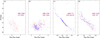 |
Fig. 1 Comparison of the CMDs of unselected (a and b) and selected (c and d) candidate tidal capture cluster pairs. The member stars of each cluster are adopted from HR23. |
2 Data
HR23 conducted a blind, all-sky search for OCs using 729 million sources from Gaia Data Release (DR) 3 down to magnitude G ~ 20, creating a homogeneous catalogue including 7167 clusters. Subsequently, Hunt & Reffert (2024) estimated the mass of each cluster member star using PARSEC (Bressan et al. 2012) isochrone fits and corrected for selection effects and unresolved binary stars. Mass functions were then fitted and integrated to calculate the total cluster mass. They then used these masses to calculate the Jacobi radius of each cluster and to distinguish between OCs and moving groups (MGs). Palma et al. (2025) based on the physical properties (total mass, age, and size) derived by Hunt & Reffert (2024) for their entire sample, estimated the tidal force exerted on each cluster by considering only close neighbours (within 50 pc). Finally, they identified 617 pairs of systems and 261 groups. In addition, they classified candidate pair systems into three categories, genetic pairs or binaries (B), tidal capture or resonance capture pairs (C), and optical pairs (O), by analysing the proper motion distribution, age and CMDs of the two sub-clusters. Since Palma et al. (2025) did not exclude MGs from their sample, many OC–MG and MG–MG combinations were included among their candidate pairs. At the same time, we find that the CMDs of many clusters within their capture pairs do not follow a clear isochrone, but instead exhibit a dispersed and disordered structure (see Figs. 1a and 1b). This complicates the determination of the precise ages of the clusters through isochrone fitting. On the one hand, we excluded those capture pairs that include MGs; on the other hand, we carefully examined the CMDs of the remaining pairs within the binary plot. Finally, we selected two pairs of clusters that follow clear isochrones and exhibit significant age differences as our study sample: ASCC 71 and ESO 064-05, and NGC 2129 and UBC 437 (see Figs. 1c and 1d). The candidate tidal capture binary cluster ASCC 71 and ESO 064-05 (Fig. 2) are located in the Carina region of the Galactic disk, slightly below the Galactic plane, at heliocentric distances of about 1.3 kpc. NGC 2129 and UBC 437 are situated close to the Galactic anti-centre direction in Gemini, essentially on the Galactic plane, at heliocentric distances of about 2.1 kpc.
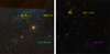 |
Fig. 2 Digitized Sky Survey 2 colour images showing the positions and morphologies of the two candidate tidal capture clusters. Squares of different colours represent the member stars of each cluster employed in this work. |
3 Method
3.1 Cluster memberships
To improve the reliability of the cluster membership, we referred to the cluster data provided by HR23 to re-retrieve the member stars of each cluster. HR23 provides the latest property parameters (![Mathematical equation: $\[\alpha, \delta, \mu_\alpha^*, s_{\mu_\alpha^*}, \mu_\delta, s_{\mu_\delta}, \varpi, s_{\varpi}\]$](/articles/aa/full_html/2025/10/aa56624-25/aa56624-25-eq9.png) , and rtot) for each cluster. The relative errors in parallax were restricted to within 10% to ensure data quality. Furthermore, we employed the re-normalised unit weight error (RUWE; Lindegren et al. 2021b) to further refine our selection. The astrometric and photometric selection criteria applied to the Gaia Archive data for each cluster are as follows:
, and rtot) for each cluster. The relative errors in parallax were restricted to within 10% to ensure data quality. Furthermore, we employed the re-normalised unit weight error (RUWE; Lindegren et al. 2021b) to further refine our selection. The astrometric and photometric selection criteria applied to the Gaia Archive data for each cluster are as follows:
Centred on the cluster position (α, δ) within a radius of rtot;
![Mathematical equation: $\[\mu_\alpha^* \pm 5 s_{\mu_\alpha^*}; \mu_\delta \pm 5 ~s_{\mu_\delta}\]$](/articles/aa/full_html/2025/10/aa56624-25/aa56624-25-eq10.png) ;
;ϖ ± 3 sϖ;
parallaxovererror >10;
RUWE < 1.4.
Based on the initial sample, we employed the Density-Based Spatial Clustering of Applications with Noise (DBSCAN) algorithm (Ester et al. 1996) to recover the clusters, as numerous studies have demonstrated the efficacy of DBSCAN in identifying OCs (Castro-Ginard et al. 2022). To verify the reliability of the cluster membership identified by DBSCAN, we compared our results with the member stars listed in the catalogue of Cantat-Gaudin & Anders (2020). Cantat-Gaudin & Anders (2020) provided member candidates for 2017 OCs based on Gaia DR2, all with membership probabilities greater than or equal to 0.7. We matched 68, 0, 56, and 25 member stars for the clusters ASCC 71, ESO 064-05, NGC 2129, and UBC 437, respectively. According to the catalogue of Cantat-Gaudin & Anders (2020), the corresponding numbers of member candidates for these clusters are 76, 0, 73, and 32, respectively. A comparison between our member candidates and those provided by Cantat-Gaudin & Anders (2020) reveals a good level of agreement between the two membership lists. Some member candidates identified by Cantat-Gaudin & Anders (2020) are not included in our list. We find that most of the excluded stars have large parallax errors and therefore do not meet our selection criteria.
3.2 Fundamental parameter
To estimate the ages of the OCs, we performed isochrone fitting on the CMD of each target, using theoretical isochrones in the Gaia photometric system from PARSEC v1.2S (Bressan et al. 2012). These isochrones cover 15 metallicities (Z = 0.0001, 0.0002, 0.0005, 0.001, 0.002, 0.004, 0.006, 0.008, 0.01, 0.014, 0.017, 0.02, 0.03, 0.04, and 0.06) and 1200 ages ranging from 1 to 5996 Myr in steps of 5 Myr. The fitting was carried out with our updated version of the Powerful CMD code (Li et al. 2017). The code divides the CMD of star clusters into 1500 cells, including 50 colour bins and 30 magnitude bins, and employs the weighted average difference (WAD) to evaluate the goodness of fit (Deng & Li 2024; Li & Zhu 2025). The WAD is calculated using the formula
![Mathematical equation: $\[\mathrm{WAD}=\frac{\sum \omega_i\left|f_{\mathrm{ob}}-f_{\mathrm{th}}\right|}{\sum \omega_i},\]$](/articles/aa/full_html/2025/10/aa56624-25/aa56624-25-eq11.png) (1)
(1)
where ωi is the weight of the ith cell, and fob and fth are star fractions of observed and theoretical CMDs in the same cell, respectively. The parameters of stellar population models with the lowest WAD value were taken as the best-fit results. The fitting results are shown in Fig. 3. The ages of ASCC 71, ESO 064-05, NGC 2129, and UBC 437 are ![Mathematical equation: $\[136_{-40}^{+95}\]$](/articles/aa/full_html/2025/10/aa56624-25/aa56624-25-eq12.png) Myr,
Myr, ![Mathematical equation: $\[56_{-5}^{+15}\]$](/articles/aa/full_html/2025/10/aa56624-25/aa56624-25-eq13.png) Myr,
Myr, ![Mathematical equation: $\[46_{-20}^{+115}\]$](/articles/aa/full_html/2025/10/aa56624-25/aa56624-25-eq14.png) Myr, and
Myr, and ![Mathematical equation: $\[426_{-135}^{+570}\]$](/articles/aa/full_html/2025/10/aa56624-25/aa56624-25-eq15.png) Myr, respectively. ASCC 71 and ESO 064-05 exhibit an age difference of approximately 80 Myr, whereas the difference between NGC 2129 and UBC 437 is significantly larger, at around 380 Myr. Such a significant age difference suggests that these two pairs of clusters are not primordial. Simultaneously, the isochrone fits also yield the metal abundance, distance modulus, and colour excess for each cluster, as presented in Table 1.
Myr, respectively. ASCC 71 and ESO 064-05 exhibit an age difference of approximately 80 Myr, whereas the difference between NGC 2129 and UBC 437 is significantly larger, at around 380 Myr. Such a significant age difference suggests that these two pairs of clusters are not primordial. Simultaneously, the isochrone fits also yield the metal abundance, distance modulus, and colour excess for each cluster, as presented in Table 1.
Based on the cluster’s member star data, we used Gaussian fits to derive the mean and standard deviation values of each cluster’s position and proper motion. In addition, we corrected the parallax zero point for all member stars using the code from Lindegren et al. (2021a), subsequently obtaining the mean parallax and standard deviation for each cluster. While Gaia DR3 provides complete astrometric and photometric data for our sample of stars, only a small fraction of the radial velocity (RV) data is available. Particularly for UBC 437, no member star contains RV data. Therefore, we incorporated the Large Sky Aera Multi-object Fiber Spectroscopic Telescope (LAMOST) DR11 low-resolution archive (Luo et al. 2012; Zhao et al. 2012), which contains RV data for nearly eight million stars. Cross-matching was subsequently performed using Topcat (Taylor 2005) based on 2D star coordinates. LAMOST DR 11 provides RV data for 0, 0, 15, and 20 member stars of ASCC 71, ESO 064-05, NGC 2129, and UBC 437, respectively. In cases where both surveys provide RV measurements for the same star, we adopted the value with the lower relative error. The average RVs and their associated uncertainties for each cluster were calculated using the weighting scheme described by Soubiran et al. (2018). The average RV was obtained using the following formula:
![Mathematical equation: $\[R V_{\mathrm{OC}}=\frac{\sum_i R V_i \times w_i}{\sum_i w_i},\]$](/articles/aa/full_html/2025/10/aa56624-25/aa56624-25-eq16.png) (2)
(2)
where wi is defined as wi = 1/(ϵi)2, and RVi and ϵi are the RV and RV error for the star i provided in Gaia DR3 and LAMOST DR11. The internal error of RVOC is defined as
![Mathematical equation: $\[I=\frac{\sum_i w_i \times \epsilon_i}{\sum_i w_i},\]$](/articles/aa/full_html/2025/10/aa56624-25/aa56624-25-eq33.png) (3)
(3)
and the weighted standard deviation σRVOC of RVOC is defined as
![Mathematical equation: $\[\sigma_{R V_{\mathrm{OC}}}=\sqrt{\frac{\sum_i w_i}{\left(\sum_i w_i\right)^2-\sum_i w_i^2} \times \sum_i w_i \times\left(R V_i-R V_{\mathrm{OC}}\right)^2}.\]$](/articles/aa/full_html/2025/10/aa56624-25/aa56624-25-eq34.png) (4)
(4)
The RVOC uncertainty is defined as the maximum of the standard error ![Mathematical equation: $\[\sigma_{R V_{\mathrm{OC}}} / \sqrt{N}\]$](/articles/aa/full_html/2025/10/aa56624-25/aa56624-25-eq35.png) and
and ![Mathematical equation: $\[I / \sqrt{N}\]$](/articles/aa/full_html/2025/10/aa56624-25/aa56624-25-eq36.png) (Jasniewicz & Mayor 1988), where N is the number of star members in the cluster. To mitigate the effect of binaries on the cluster RVOC, we iteratively excluded stars with velocities outside the RVOC ± 3 × σRVOC range (Carrera et al. 2022; Qin et al. 2025). The fundamental parameters of each cluster are listed in Table 2.
(Jasniewicz & Mayor 1988), where N is the number of star members in the cluster. To mitigate the effect of binaries on the cluster RVOC, we iteratively excluded stars with velocities outside the RVOC ± 3 × σRVOC range (Carrera et al. 2022; Qin et al. 2025). The fundamental parameters of each cluster are listed in Table 2.
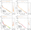 |
Fig. 3 CMDs of ASCC 71, ESO 064-05, NGC 2129, and UBC 437. The black dots represent the member stars of the cluster from Gaia DR3. The magenta points represent the best-fit ages obtained from the PARSEC isochrones, and the green and orange points represent the upper and lower limits of age. The right and top panels of each subplot display the differences in magnitude and colour between the observational data and the isochrones, with the best-fitting isochrone exhibiting the smallest deviation. |
Fundamental parameters of the four clusters.
3.3 Correction for distance
The apparent elongation of the cluster morphology along the line of sight has been observed in many cases (Pang et al. 2020; Ye et al. 2021; Qin et al. 2023a). This elongation is artificially caused by directly using the reciprocal of parallax as the distance (Qin et al. 2023a). Because parallax errors follow a symmetric distribution, taking the reciprocal leads to an asymmetric distribution of distances (Pang et al. 2020). To mitigate this artificial elongation, we applied the Bayesian inversion method of Bailer-Jones (2015), using the prior from Carrera et al. (2019) to compute the likelihood. The prior consists of two parts, one representing the exponentially decreasing volume density for field stars, and the other representing the Gaussian spatial distribution of star cluster members. The prior is given by the following formula:
![Mathematical equation: $\[P(d) \propto C \cdot d^2 e^{-\frac{d}{8 \mathrm{[kpc]}}}+(1-C) \cdot \frac{1}{\sqrt{2 \pi \sigma_d^2}} e^{-\frac{\left(d-d_0\right)^2}{2 \sigma_d^2}},\]$](/articles/aa/full_html/2025/10/aa56624-25/aa56624-25-eq37.png) (5)
(5)
where d0 is the predicted mean distance of cluster members, adopted as the inverted parallax of clusters. σd is the deviation of the distances between member stars and their cluster centre. 1-C is the member stars probability derived by pyUPMASK (Pera et al. 2021). Assuming that the parallax uncertainty is Gaussian, the likelihood is
![Mathematical equation: $\[P(\varpi {\mid} d) \propto \mathrm{e}^{-\left(\varpi-\frac{1}{d}\right)^2 / 2 \sigma_{\varpi}^2},\]$](/articles/aa/full_html/2025/10/aa56624-25/aa56624-25-eq38.png) (6)
(6)
where ![Mathematical equation: $\[\sigma_{\varpi}^{2}\]$](/articles/aa/full_html/2025/10/aa56624-25/aa56624-25-eq39.png) equal to the quoted error bar on each parallax measurement (Carrera et al. 2019). In Fig. 4, we present the spatial distribution of member stars after applying the distance correction. The Bayesian distance estimates for ASCC 71, ESO 064-05, NGC 2129, and UBC 437 are 1338.85 ± 23.72 pc, 1334.58 ± 18.35 pc, 2090.53 ± 64.71 pc, and 2083.12 ± 70.39 pc, respectively.
equal to the quoted error bar on each parallax measurement (Carrera et al. 2019). In Fig. 4, we present the spatial distribution of member stars after applying the distance correction. The Bayesian distance estimates for ASCC 71, ESO 064-05, NGC 2129, and UBC 437 are 1338.85 ± 23.72 pc, 1334.58 ± 18.35 pc, 2090.53 ± 64.71 pc, and 2083.12 ± 70.39 pc, respectively.
Based on the corrected distance, we computed the Galactocentric coordinates (X, Y, Z) and Galactic-space velocity components (U, V, W) with the astropy Python package (Astropy Collaboration 2013, 2018) and the transformation matrix given in Johnson & Soderblom (1987), as shown in Table A.1. We adopted a distance of 8.3 kpc from the Sun to the Galactic centre and a height of 27 pc above the Galactic plane (Tang et al. 2019). The relative motion of the Sun with respect to the Galactic centre is taken as (12.9, 245.6, 7.78) km s−1 (Piatti & Malhan 2022). The 3D spatial separation between ASCC 71 and ESO 064-05 is merely 24.54±16.63 pc, and that between NGC 2129 and UBC 437 is 54.84±20.95 pc.
3.4 Radial density profile
The radial density distribution is an effective tool for studying the spatial distribution as well as the morphology of clusters. To explore the structural parameters, core radius and tidal radius of each cluster, we fitted the radial density distribution of each cluster using King (King 1962) and EFF (Elson et al. 1987) analytic templates, respectively. To do this, we drew concentric rings at the same intervals with the centre of the cluster as the origin. We calculated the stellar density in each concentric ring as ρi = Ni/Ai, where Ni is the number of stars in the i-th ring and Ai is the area of the i-th ring.
The formulas for the King and EFF analysis templates are as follows:
For the King model,
![Mathematical equation: $\[\rho(r)=\rho_{\mathrm{bg}}+\rho_0\left[\frac{1}{\sqrt{1+\left(\frac{r}{r_c}\right)^2}}-\frac{1}{\sqrt{1+\left(\frac{r_t}{r_c}\right)^2}}\right]^2,\]$](/articles/aa/full_html/2025/10/aa56624-25/aa56624-25-eq40.png) (7)
(7)
where ρbg is the background density, and ρ0 and rc are the centre density and core radius of the cluster. rc is defined as the distance when the density of the star is half the density of the centre, ρ(rc) = ρ0/2. The tidal radius is defined as the positions at which the density of the star is equal to the background density, ρ(rt) = ρbg.
For the EFF model,
![Mathematical equation: $\[\rho(r)=\rho_0\left[1+\left(\frac{r}{r_c}\right)^2\right]^{-\eta / 2},\]$](/articles/aa/full_html/2025/10/aa56624-25/aa56624-25-eq42.png) (8)
(8)
where ρ0 and rc are the same as defined in the King model. η is the slope of the EFF template for radii much larger than rc.
These empirical formulas have been widely used for analysis of the radial density profile of star clusters (Carrera et al. 2019; Haroon et al. 2024; Hu et al. 2025). The fitting results are displayed in Fig. 5. The density uncertainty in each ring was derived from Poisson statistics. The core radii driven by the King (EFF) model for each cluster is 2.56 ± 1.19 (4.09 ± 1.47), 1.82 ± 2.18 (1.52 ± 1.76), 1.31 ± 0.41 (1.52 ± 0.71), and 2.43 ± 1.16 (2.43 ± 1.09) pc, respectively. To measure the fitting performance of the two models, we calculated the chi-square value for each model fit to the clusters. The chi-square values for the fits using the King and EFF models were 14.18 (14.39), 9.50 (9.34), 9.14 (14.48), and 4.92 (4.95), respectively. Overall, the King model fits better than the EFF, and thus we took the core radius inferred by the King model as the core radius of the cluster.
Although the King model shows good performance in inferring the core radius of each cluster, the tidal radius inferred by the King model is not robust. In this study we therefore did not adopt the tidal radius derived from the King model. We adopted the same approach as Hu et al. (2025), defining the tidal radius of the cluster as the intersection point of the fitted King and EFF model curves. In this manner, we obtained tidal radii of 14.91, 13.31, 10.77, and 12.56 pc for each cluster, respectively. In addition, HR23 reported tidal radii of 11.74, 9.78, 9.96, and 8.96 pc for the respective clusters. All of our derived values are larger than those reported by HR23. Several structural parameter studies of star clusters have indicated that the tidal radii reported by HR23 may be underestimated (Tarricq et al. 2022; Hu et al. 2025). Hunt & Reffert (2024) indicates that the average tidal radius of the cluster near the solar circle is approximately 19 pc (Hu et al. 2025). Our estimate of the tidal radius more closely matches this value. Therefore, the tidal radii presented in our work are likely to be more reliable.
Property parameters of the four clusters.
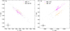 |
Fig. 4 Spatial distribution of the four clusters in the Galactocentric Cartesian coordinate system on the X–Y plane. The magenta and cyan dots represent stars after distance correction via the Bayesian approach, and the grey dots represent stars generated using the parallax inverse as the distance. |
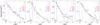 |
Fig. 5 Radial density profile in 2 D spatial space for each cluster. The red and blue curves represent King and EFF templates, respectively. The dashed magenta and green lines represent the core radii derived from fitting the radial density distribution of the clusters with the King and EFF templates. The dashed grey line indicates the intersection of the King and EFF templates, representing the tidal radius of the cluster in this work. |
 |
Fig. 6 Two pairs of cluster past and future 100 Myr orbital integration using Galpy. Pentagrams (stars) represent the position of each cluster at birth, and triangles represent the present position. Circles represent positions 100 Myr later, and dotted lines depict the trajectory from the present to the future. |
3.5 Trajectories of star clusters
To investigate the physical origins of the two cluster pairs and their future dynamical evolution, we integrated the orbits of all four clusters both backwards and forwards in time, using observational parameters including central coordinates (α, δ), proper motions (![Mathematical equation: $\[\mu_{\alpha}^{*}, \mu_{\delta}\]$](/articles/aa/full_html/2025/10/aa56624-25/aa56624-25-eq43.png) ), RVs, ages, and heliocentric distances. We used the axisymmetric Galactic potential model MWPotential2014, implemented in the Python package Galpy (Bovy 2015), to compute the orbital trajectories of the clusters. This potential consists of a bulge modelled with a power-law density profile, a Miyamoto–Nagai disk (Miyamoto & Nagai 1975), and a dark matter halo described by a Navarro–Frenk–White profile (Navarro et al. 1996).
), RVs, ages, and heliocentric distances. We used the axisymmetric Galactic potential model MWPotential2014, implemented in the Python package Galpy (Bovy 2015), to compute the orbital trajectories of the clusters. This potential consists of a bulge modelled with a power-law density profile, a Miyamoto–Nagai disk (Miyamoto & Nagai 1975), and a dark matter halo described by a Navarro–Frenk–White profile (Navarro et al. 1996).
Figure 6 shows the trajectories of these two pairs of clusters in the X–Y, X–Z, and Y–Z planes. The angular momentum and eccentricity of each cluster are shown in Table 3. We can see that the eccentricity of these clusters is between 0.04 and 0.07, which indicates that they follow almost circular orbits. In addition, the angular momentum of ASCC 71 and ESO 064-05 are essentially the same, suggesting that they will move together along similar orbits. However, we find that the X-component of the angular momentum (Lx) for NGC 2129 and UBC 437 is −8.55 and 1.97 km s−1 kpc, respectively, indicating that the two clusters rotate in opposite directions about the X-axis. In the Y–Z plane (Fig. 6f), NGC 2129 exhibits counterclockwise rotation around the X-axis, whereas UBC 437 rotates in a clockwise direction. This implies that these two clusters are only close encounters by chance.
The distances between the two pairs of clusters as a function of time are shown in Fig. 7. The bold black and red curves represent orbital separations calculated using mean observations data of the cluster. In addition, we used Monte Carlo (MC) simulations to estimate the uncertainty in the distances between cluster pairs. The initial parameters for orbital integration, including position, proper motion, distance, and RV, were adopted as mean values, with their associated uncertainties expressed as standard deviations. These parameters were then resampled from a Gaussian distribution. We used 1000 resampled data to perform forward and backward orbital integration, producing 1000 orbital separations of the cluster pairs (dashed grey and pink curves in Fig. 7). These two pairs of clusters initially meet at distances of 0.189 and 0.560 kpc, larger than typical molecular cloud sizes (100 pc; Heyer & Dame 2015). This indicates that they are not binary clusters of common origin. The physical distance between ASCC 71 and ESO 064-05 reaches a minimum of 23.7 pc at 2.76 Myr in the past, after which it gradually increases (Fig. 7a). The distance between NGC 2129 and UBC 437 reaches its minimum value of 0.055 kpc at the present time (Fig. 7b) and is expected to increase significantly in the future.
Figure 8 shows the probability distribution function of the orbital separations for the two cluster pairs at the birth time of the younger sub-cluster and at 100 Myr in the future. We can see that the orbital separation driven by mean parameters and the mean introduced by MC are very similar at birth time and 100 Myr. The orbital separation probability distribution function exhibit considerable dispersion in both backward and forward integrations, indicating that the orbital integration is highly sensitive to the initial conditions. It likewise suggests that the two pairs of clusters contain different formation and evolution scenarios. In particular, for ASCC 71 and ESO 064-05, the orbital separations derived from some of the MC sampled integrations exhibit oscillatory behaviour, suggesting that the two clusters are mutually orbiting a common centre of mass, thereby forming a true gravitationally bound binary cluster. In order to explore the real scenarios of the future evolution of these two pairs of clusters, in the next section we study their future evolution using N-body simulations.
Eccentricity and angular momentum of each cluster orbit.
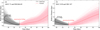 |
Fig. 7 Orbital separation between the two cluster pairs as a function of time. The bold curves represent the orbital separations between cluster pairs, calculated using the average nature parameters of the clusters listed in Table 2. The light-shaded curves represent orbital separations calculated by sampling the uncertainties in the cluster’s property parameters. |
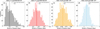 |
Fig. 8 (a and b) Histograms of ASCC 71 and ESO 064-05 orbital separations at 56 Myr ago and at 100 Myr in the future. (c and d) Histograms of NGC 2129 and UBC 437 orbital separations at 46 Myr ago and at 100 Myr in the future. The solid line represents the orbital separation calculated using the cluster mean property parameter. The dashed line represents the mean value of the orbital separation obtained using the MC sampling over the measured uncertainties in cluster property parameter. |
4 The N-body simulation
In the above section, we studied the trajectories of these two pairs of clusters in the galactic potential model by viewing the clusters as points of mass. However, their future evolutionary scenario is not clear. In this section we describe how observational data are used to generate mock clusters and to explore their future dynamical evolution, using the high-performance N-body code PETAR.
4.1 Generating mock clusters
McLuster is a powerful tool that can be used both to set initial conditions for N-body calculations and to generate simulated star clusters for direct study (Küpper et al. 2011). McLuster provides a variety of options and parameters for generating clusters with different masses, density distributions, and mass functions. Table 4 shows the input parameters to generate the mock clusters, including the mass of the cluster (M), the half-mass radius (rhm), the metal abundance (Z), the King model concentration parameter (W0), the stellar evolution time (e), the binary fraction (fb), the virial ratio (Q), and the stellar mass function.
Based on the best isochrone fitting parameters of the cluster (age, distance modulus, colour excess, and metal abundance) and the member star photometry data and uncertainties, the mass and binary fraction of the cluster was obtained from Almeida et al. (2023). The input parameters for the clusters’ metal abundances and ages were also derived from isochrone fitting. The radial density profile of star clusters follows the King model (King 1962). Using the concentration parameter of the star cluster, c = rt/rc, and the correspondence between c and W0 provided by King (1966), we obtained the concentration parameter (W0) of the star cluster, as shown in Table A.1. We calculated the half-mass radius of each star cluster using the transformation relation provided by Šablevičiūtė et al. (2006):
![Mathematical equation: $\[r_{\mathrm{hm}}=0.547 \times r_c \times\left(\frac{r_{\mathrm{t}}}{r_c}\right)^{0.486},\]$](/articles/aa/full_html/2025/10/aa56624-25/aa56624-25-eq44.png) (9)
(9)
where rc represents the core radius and rt represents the tidal radius given in Sect. 3.4. We estimated the dynamic relaxation time of each cluster using the formulae provided by Binney & Tremaine (1987):
![Mathematical equation: $\[t_{\text {relax }}=\frac{0.14 ~N \sqrt{r_{\mathrm{hm}}^3 /(G M)}}{\ln (0.4 ~N)},\]$](/articles/aa/full_html/2025/10/aa56624-25/aa56624-25-eq45.png) (10)
(10)
where M is the total mass of the cluster, N is the number of member stars, G is the gravitational constant, and rhm is the half-mass radius. The dynamic relaxation times of ASCC 71, ESO 064-05, NGC 2129, and UBC 437 were 23.97, 11.38, 7.30, and 11.78 Myr, respectively. Since the age of each cluster is significantly larger than their dynamic relaxation time, suggests that they are all in virial equilibrium (Q=0.5; Qin et al. 2025). We selected the canonical Kroupa (2001) initial mass function as the mass function of the star clusters. This initial mass function has a slope of α1 = −1.3 for stellar masses m = 0.08–0.5 M⊙, and the Salpeter (1955) slope α2 = −2.3 for m > 0.5 M⊙. Based on the parameters mentioned above, we generated four mock clusters using the McLuster procedure.
4.2 N-body simulation
The orbital integration of many particle orbits in a self-gravity bound cluster is the most appropriate method for studying the evolutionary process of the star clusters. Therefore, we employed the high-performance N-body simulation code PETAR (Wang et al. 2020) to trace the realistic evolutionary scenarios of the two cluster pairs. In the simulations, in addition to the mutual interactions between stars, we also accounted for single stellar evolution (Hurley et al. 2000) and binary stellar evolution (Hurley et al. 2002; Banerjee et al. 2020), as well as the Galactic potential (Bovy 2015). The simulation of the star clusters from present day with an evolution time of 100 Myr and generates output snapshots with a time interval of 1 Myr, which included the masses, 3D positions and velocities of each star.
Figure A.1 shows the projections of the two pairs of clusters in the X–Y and Y–Z planes at different evolutionary times (0 Myr, 5 Myr, and 10 Myr). The relative velocities of these two pairs of clusters have been in parallel directions at different evolutionary times, but they are not orbiting each other due to gravitational forces, but are rapidly moving away from each other. After 10 Myr of evolution, the distance between ASCC 71 and ESO 064-05 exceeds 40 pc, and the distance between NGC 2129 and UBC 437 exceeds 100 pc.
It has to be admitted that since we excluded stars with parallaxovererror >10, many low-mass stars were discarded, resulting in small cluster masses. This may have implications for the accuracy of the N-body simulation. We therefore regenerated the four mock clusters using the cluster masses reported by Hunt & Reffert (2024), which are 397, 108, 947, and 404M⊙, respectively (other parameters unchanged). However, the increased mass of the clusters did not affect the trajectories of the two pairs of clusters, which remained rapidly moving away from each other.
Although our simulation results indicate that in these two pairs the clusters are rapidly moving apart from each other, we could not determine whether they are currently bound. Even in the case of two clusters undergoing a hyperbolic encounter, their spatial proximity can still induce a transient but significant tidal effect (Liu et al. 2025). We can compare the orbital velocity and the RV differences (ΔRV) between clusters to determine whether they are currently bound. If they are bound, the orbital velocity corresponds to the maximum velocity difference between the two clusters. We calculated orbital velocity using the same equation as Minniti et al. (2004). The ΔRV between ASCC 71 and ESO 064-05 is 2.06 ± 0.24 km s−1, which exceeds their orbital velocity (0.26 ± 0.32 km s−1). In the case of NGC 2129 and UBC 437, the ΔRV (10.94 ± 3.37 km s−1) significantly exceeds their orbital velocity (0.20 ± 0.14 km s−1). This indicates that both pairs of clusters are currently gravitationally unbound.
5 Summary and conclusions
In general, the formation of gravitationally bound binary clusters through the close encounter of two star clusters is more likely in galaxies where the stellar velocity dispersion is relatively low, as in the Large Magellanic Cloud, where the stellar velocity dispersion is less than 20 km s−1 (Mora et al. 2019). Within the Galactic globular cluster system, low relative velocities are exceedingly rare: the characteristic velocity dispersion is ~100 km s−1 (van den Bergh 1996). However, the majority of globular clusters, both in the Magellanic Clouds (Milone et al. 2008) and in the Milky Way (Carretta et al. 2007, 2009; Pancino et al. 2010), exhibit clear evidence of multiple stellar populations. Although several theoretical models have been proposed to explain multiple stellar populations (Renzini 2008; Bastian et al. 2013), the merging of clusters with various metallicities can naturally explain the metallicity spread observed in globular clusters (Gavagnin et al. 2016). Compared with the Magellanic Clouds and dwarf spheroidal galaxies, in the Milky Way stronger tidal forces are exerted; consequently, all currently observed candidate binary clusters within the Milky Way are OCs. In recent searches for binary clusters in the Milky Way, the tidal force exerted by one cluster on a neighbouring cluster has emerged as a key indicator of binarity (Palma et al. 2025; Liu et al. 2025). The dynamical study of candidate tidal capture binary clusters undergoing mutual interactions is crucial for our understanding of the formation of multiple stellar population clusters in the Milky Way.
In this work, we investigated two pairs of tidal captured binary cluster candidates found by Palma et al. (2025), ASCC 71–ESO 064-05 and NGC 2129–UBC 437. The age difference between ASCC 71 and ESO 064-05 is ![Mathematical equation: $\[80_{-40}^{+96}\]$](/articles/aa/full_html/2025/10/aa56624-25/aa56624-25-eq46.png) Myr, the 3D distance difference is 24.54 ± 16.62 pc, and the 3D velocity difference is 2.81 ± 1.10 km s−1. The age difference between NGC 2129 and UBC 437 is even more significant, at about
Myr, the 3D distance difference is 24.54 ± 16.62 pc, and the 3D velocity difference is 2.81 ± 1.10 km s−1. The age difference between NGC 2129 and UBC 437 is even more significant, at about ![Mathematical equation: $\[380_{-136}^{+581}\]$](/articles/aa/full_html/2025/10/aa56624-25/aa56624-25-eq47.png) Myr. Their 3D distance and velocity differences are Δdist = 54.85 ± 20.96 pc and ΔV = 10.93 ± 3.32 km s−1. The age differences between the components of both pairs of clusters suggest that they are of non-common origin.
Myr. Their 3D distance and velocity differences are Δdist = 54.85 ± 20.96 pc and ΔV = 10.93 ± 3.32 km s−1. The age differences between the components of both pairs of clusters suggest that they are of non-common origin.
To investigate whether either of these two pairs of clusters will form a true gravitationally bound binary cluster through tidal capture mechanisms, we examined their trajectories and dynamical evolution based on galactic potential models and the N-body code. However, in neither pair did the clusters interact with each other, and in both cases they quickly separated after a close encounter. The orbital integrals reveal different encounter scenarios for these two pairs of clusters. ASCC 71 and ESO 064-05 were moving in similar orbits and due to the speed difference had a close encounter. The orbits of NGC 2129 and UBC 437 have similar galactocentric distances and vertical oscillation amplitudes. However, their angular momentum components along the x-axis (Lx) differ significantly in sign (−8.55 and 1.97 km s−1 kpc, respectively), indicating that they rotate in opposite directions within the Y–Z plane. This reversed orbital configuration, coupled with their similar vertical motions, contributed to a close spatial encounter.
The dynamical evolution of primordial binary clusters has been extensively studied in different configurations, such as stellar evolution, dynamical friction, and galactic tidal fields (Portegies Zwart & Rusli 2007; de la Fuente Marcos & de la Fuente Marcos 2010). In these N-body simulation works, the authors assumed primordial binary clusters moving in Keplerian orbits with different semi-major axes and eccentricities (de la Fuente Marcos & de la Fuente Marcos 2010; Darma et al. 2021). In addition to the simultaneous formation mechanism, de La Fuente Marcos & de La Fuente Marcos (2009a) proposed another formation mechanism, tidal capture. Two clusters of different ages and metal abundances can form gravitationally bound binary clusters due to tidal force interactions in close encounters. This mechanism seems more plausible in globular clusters with composite CMDs, for example NGC 1851, NGC 2808, and Fornax 3 (van den Bergh 1996).
However, most of the candidate capture pairs in the Galaxy are either flyby encounters or optical pairs (Casado 2022). Recently, Piatti & Malhan (2022) confirmed an actual collision between two individually formed star clusters (IC 4665 and Collinder 350). However, this collision did not result in a true binary cluster. Therefore, this leaves open the question of what conditions are needed for two flyby encounter star clusters to form a genuine binary cluster system.
In general, two initially gravitationally unbound objects cannot become bound during a flyby. Binary stars are not formed during two-body flybys. They are either born as binaries or become bound during three-body scattering events. Another object has to carry the excess energy away (Atallah et al. 2024), and whether this is the same for star clusters remains to be determined. The study of these issues is important for understanding the formation and evolution of star clusters.
Acknowledgements
We thank the reviewer for the valuable suggestion, which has improved the paper. We thank Qin Songmei and Tang Xican for their guidance on the research methods. This work has been supported by the National Natural Science Foundation of China (No. 12473029), China Manned Space Project (No. CMS-CSST-2021-A08), and Guanghe Fundation (No. ghfund202407013470), Dali Expert Workstation of Rainer Spurzem, Yunnan Academician Workstation of Wang Jingxiu (202005AF150025). S.H.Z. acknowledges the support from the National Natural Science Foundation of China (grant Nos. 12173026, 12141302), the Innovation Program of Shanghai Municipal Education Commission (grant No. 2025GDZKZD04), the scientific research grants from the China Manned Space Project (grant Nos. CMS-CSST-2025-A06, CMS-CSST-2025-A07), the Program for Professor of Special Appointment (Eastern Scholar) at Shanghai Institutions of Higher Learning, and the Shuguang Program (23SG39) of Shanghai Education Development Foundation and Shanghai Municipal Education Commission. This work has made use of data from the European Space Agency (ESA) mission Gaia (https://www.cosmos.esa.int/gaia), processed by the Gaia Data Processing and Analysis Consortium (DPAC, https://www.cosmos.esa.int/web/gaia/dpac/consortium). Funding for the DPAC has been provided by national institutions, in particular the institutions participating in the Gaia Multilateral Agreement.
Appendix A Input parameters and N-body simulation results
The input parameters used to generate the synthetic clusters and the results of the N-body simulations are presented in Appendix A.
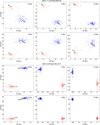 |
Fig. A.1 Future evolution of two pairs of clusters. We show the projections of the two pairs in the X–Y and Y–Z planes at different evolutionary times (0 Myr, 5 Myr, and 10 Myr). The size of the points represents the stellar mass. The green and red arrows indicate relative velocities.. |
Input parameters used to generate the mock clusters.
References
- Almeida, A., Monteiro, H., & Dias, W. S. 2023, MNRAS, 525, 2315 [NASA ADS] [CrossRef] [Google Scholar]
- Astropy Collaboration (Robitaille, T. P., et al.) 2013, A&A, 558, A33 [NASA ADS] [CrossRef] [EDP Sciences] [Google Scholar]
- Astropy Collaboration (Price-Whelan, A. M., et al.) 2018, AJ, 156, 123 [Google Scholar]
- Atallah, D., Weatherford, N. C., Trani, A. A., & Rasio, F. A. 2024, ApJ, 970, 112 [Google Scholar]
- Bailer-Jones, C. A. L. 2015, PASP, 127, 994 [Google Scholar]
- Banerjee, S., Belczynski, K., Fryer, C. L., et al. 2020, A&A, 639, A41 [NASA ADS] [CrossRef] [EDP Sciences] [Google Scholar]
- Bastian, N., Lamers, H. J. G. L. M., de Mink, S. E., et al. 2013, MNRAS, 436, 2398 [CrossRef] [Google Scholar]
- Bhatia, R. K., & Hatzidimitriou, D. 1988, MNRAS, 230, 215 [NASA ADS] [Google Scholar]
- Bica, E. L. D., Schmitt, H. R., Dutra, C. M., & Oliveira, H. L. 1999, AJ, 117, 238 [NASA ADS] [CrossRef] [Google Scholar]
- Bica, E., Pavani, D. B., Bonatto, C. J., & Lima, E. F. 2019, AJ, 157, 12 [Google Scholar]
- Binney, J., & Tremaine, S. 1987, Galactic dynamics (Princeton University Press) [Google Scholar]
- Bovy, J. 2015, ApJS, 216, 29 [NASA ADS] [CrossRef] [Google Scholar]
- Bressan, A., Marigo, P., Girardi, L., et al. 2012, MNRAS, 427, 127 [NASA ADS] [CrossRef] [Google Scholar]
- Brown, J. H., Burkert, A., & Truran, J. W. 1995, ApJ, 440, 666 [NASA ADS] [CrossRef] [Google Scholar]
- Cantat-Gaudin, T., & Anders, F. 2020, A&A, 633, A99 [NASA ADS] [CrossRef] [EDP Sciences] [Google Scholar]
- Cantat-Gaudin, T., Jordi, C., Vallenari, A., et al. 2018, A&A, 618, A93 [NASA ADS] [CrossRef] [EDP Sciences] [Google Scholar]
- Cantat-Gaudin, T., Anders, F., Castro-Ginard, A., et al. 2020, A&A, 640, A1 [NASA ADS] [CrossRef] [EDP Sciences] [Google Scholar]
- Carrera, R., Pasquato, M., Vallenari, A., et al. 2019, A&A, 627, A119 [NASA ADS] [CrossRef] [EDP Sciences] [Google Scholar]
- Carrera, R., Casamiquela, L., Carbajo-Hijarrubia, J., et al. 2022, A&A, 658, A14 [NASA ADS] [CrossRef] [EDP Sciences] [Google Scholar]
- Carretta, E., Bragaglia, A., Gratton, R. G., et al. 2007, A&A, 464, 967 [NASA ADS] [CrossRef] [EDP Sciences] [Google Scholar]
- Carretta, E., Bragaglia, A., Gratton, R., & Lucatello, S. 2009, A&A, 505, 139 [NASA ADS] [CrossRef] [EDP Sciences] [Google Scholar]
- Casado, J. 2021, Astron. Rep., 65, 755 [NASA ADS] [CrossRef] [Google Scholar]
- Casado, J. 2022, Universe, 8, 368 [NASA ADS] [CrossRef] [Google Scholar]
- Castro-Ginard, A., Jordi, C., Luri, X., et al. 2022, A&A, 661, A118 [NASA ADS] [CrossRef] [EDP Sciences] [Google Scholar]
- Darma, R., Arifyanto, M. I., & Kouwenhoven, M. B. N. 2021, MNRAS, 506, 4603 [NASA ADS] [CrossRef] [Google Scholar]
- de La Fuente Marcos, R., & de La Fuente Marcos, C. 2009a, A&A, 500, L13 [NASA ADS] [CrossRef] [EDP Sciences] [Google Scholar]
- de la Fuente Marcos, R., & de la Fuente Marcos, C. 2009b, New A, 14, 180 [Google Scholar]
- de la Fuente Marcos, R., & de la Fuente Marcos, C. 2010, ApJ, 719, 104 [CrossRef] [Google Scholar]
- De Silva, G. M., Carraro, G., D’Orazi, V., et al. 2015, MNRAS, 453, 106 [Google Scholar]
- Deng, Y.-Y., & Li, Z.-M. 2024, Res. Astron. Astrophys., 24, 065004 [Google Scholar]
- Dias, W. S., Alessi, B. S., Moitinho, A., & Lépine, J. R. D. 2002, A&A, 389, 871 [NASA ADS] [CrossRef] [EDP Sciences] [Google Scholar]
- Dieball, A., Müller, H., & Grebel, E. K. 2002, A&A, 391, 547 [NASA ADS] [CrossRef] [EDP Sciences] [Google Scholar]
- Efremov, Y. N. 1995, AJ, 110, 2757 [Google Scholar]
- Elson, R. A. W., Fall, S. M., & Freeman, K. C. 1987, ApJ, 323, 54 [Google Scholar]
- Ester, M., Kriegel, H.-P., Sander, J., & Xu, X. 1996, in Second International Conference on Knowledge Discovery and Data Mining (KDD’96), Proceedings of a conference held August 2-4, eds. D. W. Pfitzner, & J. K. Salmon, 226 [Google Scholar]
- Fellhauer, M., & Kroupa, P. 2005, MNRAS, 359, 223 [Google Scholar]
- Gaia Collaboration (Prusti, T., et al.) 2016, A&A, 595, A1 [NASA ADS] [CrossRef] [EDP Sciences] [Google Scholar]
- Gaia Collaboration (Brown, A. G. A., et al.) 2018, A&A, 616, A1 [NASA ADS] [CrossRef] [EDP Sciences] [Google Scholar]
- Gaia Collaboration (Vallenari, A., et al.) 2023, A&A, 674, A1 [NASA ADS] [CrossRef] [EDP Sciences] [Google Scholar]
- Gavagnin, E., Mapelli, M., & Lake, G. 2016, MNRAS, 461, 1276 [NASA ADS] [CrossRef] [Google Scholar]
- Haroon, A. A., Elsanhoury, W. H., Saad, A. S., & Elkholy, E. A. 2024, Contrib. Astron. Observ. Skalnate Pleso, 54, 22 [Google Scholar]
- Heyer, M., & Dame, T. M. 2015, ARA&A, 53, 583 [Google Scholar]
- Hu, Q., Li, Y., Qin, M., et al. 2025, AJ, 169, 98 [Google Scholar]
- Hunt, E. L., & Reffert, S. 2023, A&A, 673, A114 [NASA ADS] [CrossRef] [EDP Sciences] [Google Scholar]
- Hunt, E. L., & Reffert, S. 2024, A&A, 686, A42 [NASA ADS] [CrossRef] [EDP Sciences] [Google Scholar]
- Hurley, J. R., Pols, O. R., & Tout, C. A. 2000, MNRAS, 315, 543 [Google Scholar]
- Hurley, J. R., Tout, C. A., & Pols, O. R. 2002, MNRAS, 329, 897 [Google Scholar]
- Jasniewicz, G., & Mayor, M. 1988, A&A, 203, 329 [NASA ADS] [Google Scholar]
- Johnson, D. R. H., & Soderblom, D. R. 1987, AJ, 93, 864 [Google Scholar]
- Kharchenko, N. V., Piskunov, A. E., Schilbach, E., Röser, S., & Scholz, R. D. 2013, A&A, 558, A53 [NASA ADS] [CrossRef] [EDP Sciences] [Google Scholar]
- King, I. 1962, AJ, 67, 471 [Google Scholar]
- King, I. R. 1966, AJ, 71, 64 [Google Scholar]
- Kroupa, P. 2001, MNRAS, 322, 231 [NASA ADS] [CrossRef] [Google Scholar]
- Küpper, A. H. W., Maschberger, T., Kroupa, P., & Baumgardt, H. 2011, MNRAS, 417, 2300 [Google Scholar]
- Larsen, S. S. 2000, MNRAS, 319, 893 [Google Scholar]
- Li, Z.-M., & Mao, C.-Y. 2024, Res. Astron. Astrophys., 24, 055014 [Google Scholar]
- Li, Z., & Zhu, Z. 2025, A&A, 700, A280 [NASA ADS] [CrossRef] [EDP Sciences] [Google Scholar]
- Li, Z.-M., Mao, C.-Y., Luo, Q.-P., et al. 2017, Res. Astron. Astrophys., 17, 071 [Google Scholar]
- Lindegren, L., Bastian, U., Biermann, M., et al. 2021a, A&A, 649, A4 [EDP Sciences] [Google Scholar]
- Lindegren, L., Klioner, S. A., Hernández, J., et al. 2021b, A&A, 649, A2 [EDP Sciences] [Google Scholar]
- Liu, L., & Pang, X. 2019, ApJS, 245, 32 [NASA ADS] [CrossRef] [Google Scholar]
- Liu, G., Zhang, Y., Zhong, J., et al. 2025, A&A, 702, A48 [NASA ADS] [CrossRef] [EDP Sciences] [Google Scholar]
- Luo, A. L., Zhang, H.-T., Zhao, Y.-H., et al. 2012, Res. Astron. Astrophys., 12, 1243 [CrossRef] [Google Scholar]
- Mermilliod, J. C., & Paunzen, E. 2003, A&A, 410, 511 [NASA ADS] [CrossRef] [EDP Sciences] [Google Scholar]
- Milone, A. P., Piotto, G., Bedin, L. R., & Sarajedini, A. 2008, Mem. Soc. Astron. Italiana, 79, 623 [Google Scholar]
- Minniti, D., Rejkuba, M., Funes, J. G., & Kennicutt, Jr., R. C. 2004, ApJ, 612, 215 [Google Scholar]
- Miyamoto, M., & Nagai, R. 1975, PASJ, 27, 533 [NASA ADS] [Google Scholar]
- Mora, M. D., Puzia, T. H., & Chanamé, J. 2019, A&A, 622, A65 [NASA ADS] [CrossRef] [EDP Sciences] [Google Scholar]
- Navarro, J. F., Frenk, C. S., & White, S. D. M. 1996, ApJ, 462, 563 [Google Scholar]
- Palma, T., Coenda, V., Baume, G., & Feinstein, C. 2025, A&A, 693, A218 [NASA ADS] [CrossRef] [EDP Sciences] [Google Scholar]
- Pancino, E., Rejkuba, M., Zoccali, M., & Carrera, R. 2010, A&A, 524, A44 [NASA ADS] [CrossRef] [EDP Sciences] [Google Scholar]
- Pang, X., Li, Y., Tang, S.-Y., Pasquato, M., & Kouwenhoven, M. B. N. 2020, ApJ, 900, L4 [NASA ADS] [CrossRef] [Google Scholar]
- Pavlovskaya, E. D., & Filippova, A. A. 1989, Soviet Ast., 33, 6 [NASA ADS] [Google Scholar]
- Pera, M. S., Perren, G. I., Moitinho, A., Navone, H. D., & Vazquez, R. A. 2021, A&A, 650, A109 [NASA ADS] [CrossRef] [EDP Sciences] [Google Scholar]
- Piatti, A. E., & Malhan, K. 2022, MNRAS, 511, L1 [NASA ADS] [CrossRef] [Google Scholar]
- Pietrzynski, G., & Udalski, A. 1999, Acta Astron., 49, 165 [NASA ADS] [Google Scholar]
- Portegies Zwart, S. F., & Rusli, S. P. 2007, MNRAS, 374, 931 [Google Scholar]
- Qin, M. F., Zhang, Y., Liu, J., et al. 2023a, A&A, 675, A67 [NASA ADS] [CrossRef] [EDP Sciences] [Google Scholar]
- Qin, S., Zhong, J., Tang, T., & Chen, L. 2023b, ApJS, 265, 12 [NASA ADS] [CrossRef] [Google Scholar]
- Qin, S., Zhong, J., Tang, T., et al. 2025, A&A, 693, A317 [NASA ADS] [CrossRef] [EDP Sciences] [Google Scholar]
- Renzini, A. 2008, MNRAS, 391, 354 [Google Scholar]
- Šablevičiūtė, I., Vansevičius, V., Kodaira, K., et al. 2006, Baltic Astron., 15, 547 [Google Scholar]
- Salpeter, E. E. 1955, ApJ, 121, 161 [Google Scholar]
- Sim, G., Lee, S. H., Ann, H. B., & Kim, S. 2019, J. Korean Astron. Soc., 52, 145 [NASA ADS] [Google Scholar]
- Song, F., Esamdin, A., Hu, Q., & Zhang, M. 2022, A&A, 666, A75 [NASA ADS] [CrossRef] [EDP Sciences] [Google Scholar]
- Soubiran, C., Cantat-Gaudin, T., Romero-Gómez, M., et al. 2018, A&A, 619, A155 [NASA ADS] [CrossRef] [EDP Sciences] [Google Scholar]
- Subramaniam, A., Gorti, U., Sagar, R., & Bhatt, H. C. 1995, A&A, 302, 86 [NASA ADS] [Google Scholar]
- Sugimoto, D., & Makino, J. 1989, PASJ, 41, 1117 [NASA ADS] [Google Scholar]
- Tang, S.-Y., Pang, X., Yuan, Z., et al. 2019, ApJ, 877, 12 [Google Scholar]
- Tarricq, Y., Soubiran, C., Casamiquela, L., et al. 2022, A&A, 659, A59 [NASA ADS] [CrossRef] [EDP Sciences] [Google Scholar]
- Taylor, M. B. 2005, in Astronomical Society of the Pacific Conference Series, 347, Astronomical Data Analysis Software and Systems XIV, eds. P. Shopbell, M. Britton, & R. Ebert, 29 [Google Scholar]
- van den Bergh, S. 1996, ApJ, 471, L31 [Google Scholar]
- Wang, L., Iwasawa, M., Nitadori, K., & Makino, J. 2020, MNRAS, 497, 536 [NASA ADS] [CrossRef] [Google Scholar]
- Whitmore, B. C., Gilmore, D., Leitherer, C., et al. 2005, AJ, 130, 2104 [Google Scholar]
- Ye, X., Zhao, J., Zhang, J., Yang, Y., & Zhao, G. 2021, AJ, 162, 171 [NASA ADS] [CrossRef] [Google Scholar]
- Zhao, G., Zhao, Y.-H., Chu, Y.-Q., Jing, Y.-P., & Deng, L.-C. 2012, Res. Astron. Astrophys., 12, 723 [NASA ADS] [CrossRef] [Google Scholar]
All Tables
All Figures
|
Fig. 1 Comparison of the CMDs of unselected (a and b) and selected (c and d) candidate tidal capture cluster pairs. The member stars of each cluster are adopted from HR23. |
| In the text | |
|
Fig. 2 Digitized Sky Survey 2 colour images showing the positions and morphologies of the two candidate tidal capture clusters. Squares of different colours represent the member stars of each cluster employed in this work. |
| In the text | |
|
Fig. 3 CMDs of ASCC 71, ESO 064-05, NGC 2129, and UBC 437. The black dots represent the member stars of the cluster from Gaia DR3. The magenta points represent the best-fit ages obtained from the PARSEC isochrones, and the green and orange points represent the upper and lower limits of age. The right and top panels of each subplot display the differences in magnitude and colour between the observational data and the isochrones, with the best-fitting isochrone exhibiting the smallest deviation. |
| In the text | |
|
Fig. 4 Spatial distribution of the four clusters in the Galactocentric Cartesian coordinate system on the X–Y plane. The magenta and cyan dots represent stars after distance correction via the Bayesian approach, and the grey dots represent stars generated using the parallax inverse as the distance. |
| In the text | |
|
Fig. 5 Radial density profile in 2 D spatial space for each cluster. The red and blue curves represent King and EFF templates, respectively. The dashed magenta and green lines represent the core radii derived from fitting the radial density distribution of the clusters with the King and EFF templates. The dashed grey line indicates the intersection of the King and EFF templates, representing the tidal radius of the cluster in this work. |
| In the text | |
|
Fig. 6 Two pairs of cluster past and future 100 Myr orbital integration using Galpy. Pentagrams (stars) represent the position of each cluster at birth, and triangles represent the present position. Circles represent positions 100 Myr later, and dotted lines depict the trajectory from the present to the future. |
| In the text | |
|
Fig. 7 Orbital separation between the two cluster pairs as a function of time. The bold curves represent the orbital separations between cluster pairs, calculated using the average nature parameters of the clusters listed in Table 2. The light-shaded curves represent orbital separations calculated by sampling the uncertainties in the cluster’s property parameters. |
| In the text | |
|
Fig. 8 (a and b) Histograms of ASCC 71 and ESO 064-05 orbital separations at 56 Myr ago and at 100 Myr in the future. (c and d) Histograms of NGC 2129 and UBC 437 orbital separations at 46 Myr ago and at 100 Myr in the future. The solid line represents the orbital separation calculated using the cluster mean property parameter. The dashed line represents the mean value of the orbital separation obtained using the MC sampling over the measured uncertainties in cluster property parameter. |
| In the text | |
|
Fig. A.1 Future evolution of two pairs of clusters. We show the projections of the two pairs in the X–Y and Y–Z planes at different evolutionary times (0 Myr, 5 Myr, and 10 Myr). The size of the points represents the stellar mass. The green and red arrows indicate relative velocities.. |
| In the text | |
Current usage metrics show cumulative count of Article Views (full-text article views including HTML views, PDF and ePub downloads, according to the available data) and Abstracts Views on Vision4Press platform.
Data correspond to usage on the plateform after 2015. The current usage metrics is available 48-96 hours after online publication and is updated daily on week days.
Initial download of the metrics may take a while.