© The Authors 2025

1 Introduction

A growing number of exoplanets are being detected around young stars (age <50 Myr), either through transit monitoring (e.g., Mann et al. 2016; Plavchan et al. 2020; Bouma et al. 2020; Barber et al. 2024) or radial velocity measurements (e.g., Lagrange et al. 2019). Historically, however, the first young exoplanets were identified via high-contrast imaging (e.g., Chauvin et al. 2005; Marois et al. 2008; Lagrange et al. 2010; De Rosa et al. 2023). At such a young age, the continuum of a Jovian exoplanet becomes bright enough to be detected directly thanks to adaptive optics (AO), enabling instruments to reach contrasts up to 10⁻⁶ (e.g., VLT/SPHERE’ Gemini/GPI, Subaru/SCExAO; Beuzit et al. 2019; Macintosh et al. 2014; Guyon et al. 2010). Young planets are of particular interest to test the most recent predictions of formation models since they retain information about their orbital radius and composition at formation. Among that population, planets undergoing active accretion from surrounding gas provide direct constraints on formation timescales and the physics of accretion in the planetary-mass range, which is believed to set their early evolutionary pathway (the so-called hot- and cold-starts; Marley et al. 2007), spins (Batygin 2018), internal structure (Cumming et al. 2018), planet-disk migration (Pierens & Raymond 2016), and the composition and formation of exomoons (Heller & Pudritz 2015).

A handful of accreting planetary-mass companions have been discovered (Betti et al. 2023) so far. The emission lines (H_α at 6563Å, Pa_β at 12 820Å, Br_γ at 21660Å, HeI lines, etc.) are inventoried, and the characterization of line fluxes, profiles, and variability levels has begun, allowing the community to peer into the physics of accretion (e.g., Betti et al. 2022; Demars et al. 2023; Ringqvist et al. 2023; Aoyama et al. 2024). Among that sample, PDS70 stands out as a young system with two firmly established protoplanets, at ~ 170 mas and ~220 mas projected separation (Wang et al. 2021). They are both nested within the cavity of a primordial disk surrounding the host star (Keppler et al. 2018; Müller et al. 2018; Wagner et al. 2018; Haffert et al. 2019). The detection of the second planet in the system was made possible by the Multi-Unit Spectroscopic Explorer (MUSE; Bacon et al. 2010) integral field spectrograph (IFS) at the Very Large Telescope (VLT), which provides hyperspectral imaging at optical wavelengths coupled to AO (Arsenault et al. 2008; Ströbele et al. 2012). The medium resolution of MUSE (R_λ of 1770 at 4750 Å to 3590 at 9350 Å) allows us to pinpoint the narrow H_α line emission of accreting companions (e.g., Haffert et al. 2019; Eriksson et al. 2020); at the specific wavelength of the H_α emission line, the contrast with the star becomes modest (10⁻² to 10⁻³; Mordasini et al. 2017). IFS such as MUSE also provide the data diversity needed for an efficient removal of the stellar flux and stellar light scattered by circumstellar disks that can overlap the signal of the companions. Emission line fluxes and profiles of accreting companions such as PDS70 b or c can be extracted, after halo subtraction, from the MUSE data cubes. These studies have triggered new theoretical developments and provided constraints on the accretion rates, in-line extinction by surrounding material, and the physics of accretion (e.g., Aoyama & Ikoma 2019; Thanathibodee et al. 2019; Szulágyi & Ercolano 2020; Hashimoto et al. 2020; Marleau et al. 2022).

Campaigns to detect analogues of PDS70 b and c have thus far targeted H_α, Pa_β, and Br_γ emissions in young systems with circumstellar disks. Most of them have relied on differential imaging in narrow-band filters, whose transmission is centered on the line and the surrounding continuum (Cugno et al. 2019; Uyama et al. 2020; Zurlo et al. 2020; Huélamo et al. 2022; Follette et al. 2023; Chaushev et al. 2024). Reported candidates (LkCa 15 b, AB Aur b; Sallum et al. 2015; Currie et al. 2022) await confirmation. AO-fed IFS at medium spectral resolution have been used to target a few systems thus far, looking for Pa_β emissions (OSIRIS at Keck; Uyama et al. 2017, 2021; Biddle et al. 2024) as well as H_α lines (MUSE at VLT; Xie et al. 2020). Only the stellar companion around HTLup has been reported as a positive detection with MUSE, at a separation similar to the protoplanets around PDS70 (~160 mas; Jorquera et al. 2024). No new protoplanet has been reported from archival data or ongoing observations. Variability of the lines or in-line extinction from circumstellar and/or circumplanetary material are proposed to explain this poor yield (Szulágyi & Ercolano 2020; Marleau et al. 2022; Demars et al. 2023; Alarcón et al. 2024).

Hoeijmakers et al. (2018) presented a methodology named high-resolution spectral differential imaging (HRSDI) to remove the stellar light from VLT/SINFONI AO-fed IFS observations (R ~ 4000; 19 600-24 500 Å). The method was adapted by Haffert et al. (2019) and Xie et al. (2020) to work on MUSE data. However, although it is currently the reference method for planet detection and characterization from IFS data, it can distort the companion emission spectrum. Moreover, being non-linear and non-parametric, it prevents regularization and further extensions. Alternatively, spline-based models for complex halos/speckles thus have also emerged (Agrawal et al. 2023; Ruffio et al. 2023).

In that context, in Julo et al. (2024), we laid the foundations of a new halo subtraction methodology aimed at paving the way for some of the developments mentioned above. In that work, we demonstrated the feasibility of our approach, but we did not provide a more extended demonstration of its capabilities on-sky.

We build upon the study of Julo et al. (2024), and present a more thorough investigation of the biases introduced by the state-of-the-art method using an analytical approach in Sect. 2, while providing a demonstration of our method using archival and new on-sky data in Sect. 3. Then, we examine the remaining limitations and give our conclusions, remarks, future prospects in Sect. 4. A preliminary definition of the proposed model was given in Julo et al. (2024). The present paper also provides a more accurate and complete description of both methodologies in Appendix A for better understanding and reproducibility.

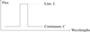Fig. 1 Toy model with rectangular line and flat neighboring continuum. companion emission spectrum. Moreover, being non-linear and non-parametric, it prevents regularization and further extensions. Alternatively, spline-based models for complex halos/speckles thus have also emerged (Agrawal et al. 2023; Ruffio et al. 2023).

2 Quantification of the biases

The HRSDI method can be decomposed into two steps:

• First, a “reference stellar spectrum” is built by averaging a selection of spaxels of the field of view. For each spaxel of the full field of view, the ratio of the data to the reference spectrum is smoothed by a low-pass Savitzky-Golay filter (to remove the high-frequency planetary components of the observations). Each of the spaxels of the field is subtracted from the product of the reference spectrum and this filtered ratio. The division and filtering problems are highlighted in the following section using a custom toy model.

• Second, principal component analysis (PCA) is used on the cube of residuals to remove static patterns in the field of view. It assumes (improperly) the relevance of a low-rank model of the companion in the post-subtraction residuals of the data, and could introduce self-subtraction of its signal.

Because of this uncontrolled self-subtraction, we prefer to avoid this second step. Therefore, we chose to focus our work on the first step and name it the Savitzky-Golay filtering (SGF) method.

2.1 Analytical study with toy models

The toy model is introduced in Fig. 1. C_S and L_S (respectively, C_P and L_P) denote the continuum and line fluxes of the stellar (respectively, planetary) component of a data spaxel. The latter thus exhibits C = C_S + C_P and L = L_S + L_P. Furthermore, C_S » C_P and L_S » L_P are assumed. These hypothesis allow us to infer the quantities C_S and L_S to a certain factor through the stellar reference spectrum. The major issue related to this step is then to evaluate this (position-dependent) factor, referred to as α (assumed locally spectrally constant in the toy model).

To achieve this, the spaxel is divided entrywise by the stellar reference spectrum, yielding the signal shown in Fig. 2a.

By neglecting the planetary continuum at flux level C_p (which is less informative than the planetary lines), h_min (which is by construction the data to stellar continuum ratio) is indeed equal to the factor α. The task then reduces to filtering the peak induced by the higher contrast planetary line at flux level L_P.

Here, this is done by low-pass (Savitzky-Golay) filtering, which results in the signal in Fig. 2b. This filtering step leaves a residue that depends on physical and processing configurations. The width of this residual is W and its height is RH, with W the filtering window width, R the ratio between the line width and the filtering window width, and H the peak height of the spaxel relative to the stellar reference spectrum. Technical details of the calculations are given in Appendix B.1.

The entrywise product of this deformation with the stellar reference spectrum gives the estimation of the stellar component of the data spaxel shown in Fig. 2c. Subtracting this estimation from the initial data spaxel gives the estimation of the planetary component of the data shown in Fig. 2d. Yet, the propagation of the artifact described in the previous steps is clearly highlighted and quantified with this toy model.

Next, we explore two extreme (but still realistic) scenarios, to better understand the limitations of this approach:

• If L_P/L_S  C_P/C_S, then $\overline{\mathrm{H}}\gg \alpha$ and consequently $\mathrm{R}\overline{\mathrm{H}}\gg \mathrm{R}\alpha$. This leads to the overfitting of the flux of the stellar spaxel defined in Fig. 2c, such that ${\tilde{C}}_S-{\hat{C}}_S\gg \mathrm{R}{C}_S$. This results, in turn, in an oversubtraction in the flux of the planetary spaxel estimate defined in Fig. 2d, such that ${\tilde{C}}_P-{\hat{C}}_P\ll -\mathrm{R}{C}_P$. This is referred to as “self-subtraction” and potentially limits the relevance of physical interpretations. Importantly, the oversubtraction is not uniform across the spectrum: this differs between line wavelengths and neighboring continuum ones (i.e., $L_S-{\hat{L}}_S\ne {\tilde{C}}_S$). Consequently, this process induces an irrecoverable loss of information (since $L_S\ne {\hat{L}}_S+{\tilde{C}}_S$).

• If L_p/L_S ≈ C_P/C_S, then $\overline{\mathrm{H}}\approx 0$ and consequently $\mathrm{R}\overline{\mathrm{H}}\approx 0$. As a result, the artifacts are negligible in the final estimates (i.e., ${\tilde{C}}_P-{\hat{C}}_P\approx 0$), but the planetary signal is minimally recovered (i.e., ${\hat{L}}_P\ll L_P$). In fact, the full process relies on the peak of the stellar spaxel to spectrum ratio: if it is too high, this leads to self-subtraction; if it is too low, this hinders the recovery of the planetary signal. This reflects the intrinsic difficulty of separating signals with similar contrast ratios.

These extreme phenomena are illustrated below (Sect. 2.2) through a few simulations. These effects compound the intrinsic numerical instabilities introduced by the division step depicted in Fig. 2a, especially at low-flux (noise-dominated) wavelengths.

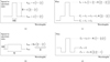Fig. 2 Signal processing steps leading to post-subtraction planetary spaxel estimates. (a) Data spaxel ratio with regard to the reference spectrum. (b) Low-pass filtering with Savitzky-Golay filter. (c) Stellar spaxel estimation with overfitting. (d) Planetary spaxel estimation with self-subtraction.

2.2 Illustration from simulations

While the reduction in line height is intrinsic to the problem of separating signals that are too close together, the self-subtraction around the line is only specific to the SGF method. Following the calculations carried out on our simple toy model, its width can simply be approximated to the width W of the Savitzky-Golay filter window. Its depth with respect to the 0 flux level, which is the expected estimation for the continuum, can be expressed as: $$\frac{{\tilde{C}}_P}{{\hat{L}}_P}=-\left(\frac{\mathrm{R}}{1-\mathrm{R}}\right)\frac{C_S}{L_S},$$(1)

where ${\hat{L}}_P$ and ${\tilde{C}}_P$, introduced in Fig. 2d, represent, respectively, the estimation of the planetary line height and the estimation of the planetary neighboring continuum depth with regard to the 0 value. The interest of Eq. (1) is to quantify the self-subtraction effect using only the post-subtraction quantities (${\hat{L}}_P$ and ${\tilde{C}}_P$) and the stellar continuum-to-line ratio, C_S/L_S (since the planetary continuum-to-line ratio, C_P/L_P, simplifies in the calculation).

This provides a generalized framework for estimating the post-subtraction residuals behavior using a limited amount of free parameters. We vetted it using more realistic simulations, as illustrated in Figs. 3, 4, and 5. They allowed us to confirm that the greater the stellar continuum-to-line ratio, C_S/L_S, the clearer the self-subtraction in the post-subtraction residuals. However, it is important to note that ${\tilde{C}}_P/{\hat{L}}_P$ reflects the self-subtraction depth, ${\tilde{C}}_P$, in relation to the line size estimate, ${\hat{L}}_P$, not only to the selfsubtraction depth, ${\tilde{C}}_P$ As a consequence, in addition to being more pronounced when the line of the stellar spectrum, L_S , is small compared to its continuum, C_S, this effect is also more pronounced when the line of the planetary spectrum, L_P (likely approximately equal to ${\hat{L}}_P$), is high (relative to the noise level). Furthermore, it is also important to note that this indicator only expresses the depth of the self-subtraction in relation to the line size estimate, ${\hat{L}}_P$, not to the true line size, L_P. Thus, although it may be counter-intuitive, the deeper the self-subtraction around the line, ${\tilde{C}}_P$, and the higher the line size estimate, ${\hat{L}}_P$. Indeed, the higher the stellar line, the more the stellar spaxel resembles the planetary spaxel to a certain factor and the more intrinsically difficult the separation problem becomes, hence the lower the planetary line estimate. As a matter of fact, the self-subtraction of the neighboring continuum and the post-subtraction flux loss of the line are distinct phenomena evolving in opposition to two intrinsically linked causes.

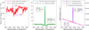Fig. 3 Subtraction results at the position of a planet with the SGF method. Left: Overlapping simulation (ground truth) and estimation of the stellar spaxel. There is no emission line in this simulation. Middle: The green spaxel is the estimation of the planetary spaxel, while the cyan one is the associated ground truth. The self-subtraction problem is clearly visible in this situation. Right: The reason for the self-subtraction is evidenced. This is the deformation estimation, in light pink, overfitting the planetary line component of the data to stellar spectrum estimation ratio, in purple. Yet, this overfitting is relatively greater than the planetary and stellar continuum-to-line ratios are different. The real deformation is in dark pink.

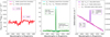Fig. 4 Same as Fig. 3, but with a small stellar line (total flux of 5 × 10−13 erg s−1 cm−2 Å−1 in the 6560.3-6565.3 Å band).

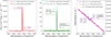Fig. 5 Same as Fig. 4, but with a brighter stellar line (total flux of 5 × 10−12 erg s−1 cm−2 Å−1 in the 6560.3-6565.3 Å band).

3 Application on VLT/MUSE data

To limit the self-subtraction effect caused by the filtering step, and the numerical errors caused by the division step, we recently proposed in Julo et al. (2024)¹ an alternative halo subtraction technique based on a linear parametric model of the chromatic deformation of the halo. The estimates of the stellar spaxels are polynomial modulations of an estimate of the stellar spectrum minimizing the distance with the data in the least squares sense. The numerical errors caused by matrix inversion are mitigated using orthogonal Legendre polynomials, while the direct use of the analytical solution enables H_α line masking to avoid the selfsubtraction caused by planetary flux overfitting in the estimate of the stellar component. Details are presented in Appendix A for better understanding and reproducibility. We name this method the Legendre polynomial modulation (LPM) method.

In this section, we illustrate multiple operating scenarios of this new method with real data, notably in order to highlight its performance with regard to detection and characterization. It is also the opportunity to illustrate the new understanding of the subtraction process that this method brings, notably through three ways for selecting the polynomial degree of modulation.

3.1 Description of on-sky data

3.1.1 Archival data of the PDS70 and HTLup systems

We re-analyzed the archival observations of PDS70 and HTLup, obtained, respectively, on June 20, 2018 (program 60.A-9100) and March 25, 2021 (program 106.21EN), with the narrow field mode of MUSE (MUSE-NFM) located at the VLT/UT4 (Bacon et al. 2010). Details of the observation sequences can be found in Haffert et al. (2019) and in Jorquera et al. (2024). Raw data were calibrated using the ESO MUSE pipeline, version 2.8 (Weilbacher et al. 2020). It produced 6 cubes of PDS70 observations and 11 cubes of HTLup observations calibrated in wavelengths (the data used are summed up in the Appendix C). All data cubes have, approximately, a squared field of view of 7.5 x 7.5” with square spaxels of 25 × 25 mas, covering the 4750—9350 À wavelength interval with spectral channels of 1.25 À in width. The host stars were approximately centered at target acquisition.

The custom routines described in Jorquera et al. (2024) have been used to measure the star position in each cube slice since it is known to drift with wavelength due to the partial correction of atmospheric refraction by the instrument and its atmospheric dispersion compensator. The star was later shifted to a common position at the center of the field of view.

3.1.2 New investigation of the YSES1 system

YSES1 (TYC 8998-760-1) is a young (16.7 ± 1.4 Myr) solarmass star with a K3 spectral type, around which 14 ± 3 M_Jup (YSES1 b) and 6 ± 1M_Jup (YSES1 c) companions have been identified at projected separations of 160AU (1.71”) and 320AU (3.37j), respectively (Bohn et al. 2020a,b). Spectroscopy at K band revealed that YSES1 b displays a faint Br_γ emission line (2.16 μm) indicative of active accretion (Zhang et al. 2021). JWST observations of YSES1 revealed excess infrared emission produced by a disk around the b planet, strengthening accretion as the origin of the emission line, but could not identify one around the c planet (Hoch et al. 2025).

We observed the YSES1 system with the VLT/MUSE-NFM on April 27, 2023 (program 109.22YA). We recorded 9 x 300 s exposures, with the field of view being rotated by 45° between exposures to filter out static features related to the slicer at the data reduction step. We followed the same reduction procedure as above to produce 9 new data cubes calibrated in wavelengths. The star is centered and corrected from the barycentric velocity.

3.2 Hyperparameters and parameters selection

A summary of the two sets of parameters of the two stellar halo subtraction methods is presented in Table 1. Firstly, the stellar spectrum estimate was made using a set of spaxels excluding both the least bright ones (as noisier) and the most bright ones (as most likely distorted by the MUSE pipeline). The spaxels were selected by comparing their total flux, F_xy (determined by spectral integration), with the maximum of the total fluxes, F_max. Secondly, we chose to select only a given wavelength interval in order to reduce the risk of polynomials being disturbed by abnormal spectrum distortions (particularly because of abusive interpolations by the MUSE pipeline when pixels are considered to be outliers). Arbitrarily, the lower bound of the kept selected spectral window was set to the upper bound of the AO band, and its upper bound was chosen so that the H_α line was centered.

Moreover, the LPM method being parametric, the H_α line could be masked too (note that the same could be done by rewriting the Savitzky-Golay in a parametric form). Thirdly, SGF parameters were set as indicated in Haffert et al. (2019), namely, with a firstorder Savitzky-Golay filter, with a degree d = 1 and a window width $\overline{\mathrm{W}}=101$ spectral channels (~126.25 Å). As for the LPM method, the hyperparameter, ∂ (i.e., the polynomial degree of the modulation), was set as per the results of Sects. 3.2.1, 3.2.2, and 3.2.3, i.e., following analytical results (with applications to simulations mimicking real data as much as possible) and on-sky data results (thanks to the interpretability results given by the orthogonality of the Legendre polynomials, with decomposition of real data). In any case, this leads to the consensus: ∂ = 4.

After subtracting the stellar halo of the different expositions, the noise was reduced by median of the residual cubes.

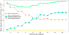Fig. 6 MSE decomposition at planet position at Hα line wavelength, following Eq. (B.5). The MSE (solid green line) is the sum of the noise overfitting error (dashed yellow line), planets overfitting error (dashdot-ted turquoise line), and star underfitting error (dotted orangy line).

3.2.1 Tuning from analytical expressions and simulations

The polynomial degree, ∂, is the key hyperparameter that must be correctly adjusted for good stellar contribution estimation (see Appendix A.4). An underestimation of the stellar contribution is caused by overly small values of ∂ as the model is too simple and underfits the deformation of the stellar spectrum estimation giving the stellar spaxel. Conversely, too large values of ∂ lead to the overestimation of the planetary contribution (and thus lead to oversubtraction). Setting the hyperparameter, ∂, consequently amounts to solving a critical bias-variance trade-off. The strategy adopted here to set the hyperparameter, ∂, consists in minimizing the mean square error (MSE). As detailed in Appendix B.2.2, this latter is analytically decomposable into three components.

In a simulated framework, each component is actually known and the MSE can be evaluated from the simulated data and the analytical expression of the post-subtraction residuals. It can even be shown (see Eq. (B.5)) that data modeled as the sum of three components (star, planets, and noise) lead to an MSE that is decomposable into three (associated) components. These errors are, respectively, named “star underfitting error,” “planets overfitting error,” and “noise overfitting error.” With the simulation described in Appendix E and the masks chosen as in the Table 1 (to be consistent with real data subtractions), MSE as a function of the degree, ∂, can be plotted as shown in Fig. 6. Firstly, from a theoretical point of view, such a decomposition confirms the expected behavior of the MSE with regard to ∂, particularly with the star underfitting error decreasing with ∂ and the planets overfitting error increasing with ∂. Secondly, from a more practical point of view, the curve also indicates that the minimization of the MSE is achieved for polynomial degrees, ∂, between 4 and 7 (in slightly equivalent ways), under these conditions. Although the simulation is a simplified version of real data, it is expected that it is sufficient to transfer these results to real data processing. Then, the simplest of these valid models can be selected: ∂ = 4.

We note, however, that the optimal value of ∂ depends on both the data and the masks used. Firstly, the stellar spaxel to stellar spectrum deformation depends on many parameters, from the observing conditions to the target used for tip-tilt sensing and even the use of the pipeline. Secondly, the set of spaxels used for the estimation of the stellar spectrum as well as the number of spectral channels used for the stellar spaxel estimation change the complexity of the model to be used, and, equivalently, the degree, ∂, of the polynomial to be used. Consequently, in order to optimize subtraction performances, all of the analysis described in this section should be done for each dataset and questioned in light of its final results.

3.2.2 Tuning from on-sky data and PSF decomposition

In addition to mitigating numerical errors, the orthogonality of the Legendre polynomials improves the interpretability of the polynomial coefficients estimated to model the stellar nuisance. By doing so, each Legendre polynomial coefficient expresses only one frequency component (in the spectral direction) of the spatial point spread function (PSF). To have a complete view of this decomposition, the median cube of 4 observations of the PDS70 system (see Appendix C for details) was processed with the LPM method with Legendre polynomials of degree ∂ = 9 (to extend the decomposition), and over the full range of wavelengths (except those around the H_α line). Fig. 7 shows the maps of the obtained coefficients, with some color-scale saturations for illustration purposes. The adaptive optics radius, the diffraction spikes, the Airy disk (core and secondary rings), as well as other patterns are decomposed in this way. Knowing that adding a higher degree polynomial to the Legendre basis does not change the estimated values taken by the coefficients of the lower-degree polynomials (thanks to their orthogonality), this gives, this time, a physical argument for the choice of the polynomial degree, ∂. This confirms the relevance of the choice: ∂ = 4. Beyond that, the modulation is just adjusting ever fainter secondary rings of the Airy disk (with low coefficient values). Moreover, we note that the circularity of most patterns justifies the treatments on successive nested rings presented in the following. Ultimately, this decomposition would help to regularize (both spatially and spectrally) the stellar estimation problem, e.g., by constraining the values of these coefficients.

3.2.3 Tuning from estimated polynomial coefficients

To go a step further and quantify the results of Sect. 3.2.2, we calculated, degree by degree, the energy of the coefficients (i.e., the sum over the field of their squared values) to understand their relative importance. Once again, the polynomials of the chosen basis being orthogonal, these energies are related to the given data cube and not to the degree of modulation used. Fig. 8 shows these calculations for several systems. The optimal polynomial degree being above all linked to the physical behavior of the PSF, all trends are similar from one observation to another. Again, among these different choices, the best one is: ∂ = 4. Beyond that, the coefficients take on the same orders of magnitude as those for very large degrees, namely, those that only fit the noise.

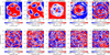Fig. 7 Maps of the polynomial coefficients of estimation of the stellar spaxels of real data of observation of the PDS70 system. The color scale is saturated at the 25% and 75% quartiles and centered on 0 by extension in the negative or in the positive (except for the degree of 0 coefficient as corresponding to the total flux). For each spaxel, before estimating the coefficients, each modulation by the base polynomials is L2 normalized (after subtraction of the average, except for the degree of 0, responsible for the total flux). Various spatial components of the PSF are identifiable thanks to the orthogonality of the polynomial basis used. Notably, the degree of 0 and 1 coefficient maps reveal the diffraction spikes in addition to the AO radius, the degree of 2 and 3 coefficient maps reveal other related patterns as well as the heart of the Airy disk, and the degree of 4 and more coefficient maps reveal the secondary rings of the Airy disk (with their outward displacement as the degree of the polynomial increases).

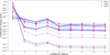Fig. 8 Energy share curves of the estimated polynomial coefficients for each of the degrees (except that of degree of 0 as accounting for the total flux and not for the variations) of the basis of decomposition. Before estimating each of the coefficients (except that of degree of 0), the modulations by the base polynomials are, firstly, subtracted from their average, secondly, L2 normalized. For each degree, the energy share is calculated as the median over the field of view of the squared coefficients, divided by the sum of all the median squared coefficients (except that of degree of 0). This was done for PDS70, HTLup, and YSES1 data cubes, each time for individual exposure. This shows that the degree of 4 polynomial coefficients are the last useful ones. Above, the energy of the high-degree coefficients converges towards a minimum where it is mainly fitting noise. It can be seen here that this minimum is reached for the degree of 5 for each of the 23 observations data, indicating that this choice may well generalize.

3.3 Impact on detection: The planetary system PDS70

3.3.1 Matched filtering

The protoplanets PDS70 b and c were detected with the two methods at H_α wavelengths. Spatio-spectral matched filtering was proposed to reduce the (symmetric) noise, in order to push the detection limits even further, using the spectral and spatial a priori that were unused by the spaxel-by-spaxel subtraction.

Fig. 9 illustrates the similar detection capabilities of the two considered methods. These are confirmed in the general case in Sect. 3.3.3 thanks to ROC curves built from these same maps (and exploring the precision-return trade-off).

To model the H _α line, a Gaussian with a 3 spectral channels (~3.75 Å) full width at half maximum (FWHM) is chosen for the spectral model. The wavelength of the latter being known, the first step is therefore the dot product of each of the spaxels of the median residual cube with this spectral model centered on the wavelength of the H_α line (~6562.8 A). To model the associated spatial PSF, the spatial model is derived from the dot product of the spaxels of the pre-subtraction cube with the spectral model; indeed, under the small-field hypothesis, the star spreads are the same as those of the planets (with planets and noise being minor compared with the star). Both models are normalized to 1.

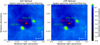Fig. 9 Spatio-spectral match filtering of the median PDS70 data cube, after stellar halo subtraction by the SGF (left) and LPM (right) methods. A Gaussian is chosen for the spectral model to search for Hα line signal. The corresponding pre-subtraction monochromatic images are chosen for the spatial model to search for spatial PSF patterns.

3.3.2 Contrast curves

Following Xie et al. (2020), we constructed the contrast curves from fake planet injections at different contrasts and separations. In practice, fake planets were injected at contrasts varying from 1 x 10⁻⁵ to 1 x 10⁻² in steps from 1 x 10⁻⁵ to 5 x 10⁻⁴. A first series of fake planet injections was done at separations varying from 0.025j to 0.5j in steps of 0.025j and at four position angles 0°, 90°, 180°, and 270°. A second series of injections was done from ~0.035j to ~0.7j in steps of ~0.035j at four other position angles 45°, 135°, 225°, and 315°. To standardize the sampling step in separation, the field of view was paved in concentric rings of pixels around the center of the images. The Andres (1994) circle tracing algorithm was used to do so. Thus, each injection could be associated with a ring, each of them being associated with a separation (by averaging the distances to the center of the pixels making up the rings). This led to as many separations as there are rings in the field of view. To test and compare both halo subtraction methods, several cubes of observation of the PDS70 system were considered (see Appendix C for more information on the cube selection) as true noise and nuisance realizations. At chosen positions and flux values, cubes containing only the fake planets were simulated according to the description given in Appendix E, and added to the real data cubes. Care was taken to inject the fake planets at positions where only noise is present in the real data cubes (i.e., far from the two protoplanet positions). Then, both stellar halo subtraction methods were applied to each of the four injected PDS70 cubes, and the residuals were merged into one median cube (for each of the injections).

Following Xie et al. (2020), the three spectral channels around the H_α line (i.e., channels 1450, 1451, and 1452) were averaged to get narrow-band images around these wavelengths; we recovered around half of the planetary fluxes as the FWHM of the spectral PSF is approximately three spectral channels. From these images, the planetary fluxes were estimated from the integration of a 3x3 pixels square centered on the positions of injection. The mean, μ, and standard deviation, σ, of the noise were estimated by integrating over the same circles, at identical separations but different angular positions than the fake planets. In practice, this comes to using pixels of the same Andres (1994) rings, but at different angular positions. The noise characteristics (i.e., μ and σ) being noticed to be varying with the wavelengths (the noise is notably more important at the H_α line wavelengths), they were estimated from the images at the H_α line wavelengths only (and not from other residuals images at other wavelengths).

To sum up, for each separation and for each flux, we have, for each of the eight angular positions, an integrated planetary flux value, and a certain number of integrated noise fluxes from which an average value, μ̂, and a standard deviation value, σ̂, can be computed. For each of these situations, the detection of an injected planet is validated if its integrated flux is greater than $\hat{\mu }+5\hat{\sigma }$, and invalidated otherwise. The contrast curves were built for each separation, by decreasing the contrast until less than half of the planets of the corresponding situation were detected (under the assumption of a symmetrical noise distribution). The contrast curve represents the minimum contrast for which more than 50% of the planets were detected. To estimate an error, the same curves were plotted for 25% and 75% detection thresholds.

The results are presented in Fig. 10. Given that the SGF method already retained almost the entire H_α line, and that the LPM method is based on the same principles as the former, it was expected that the detection limits would not be significantly improved. Yet, despite the lack of noise diversity preventing any sound conclusions, it seems that the detection performance is slightly improved. As a matter of fact, the new method improves the integrity of the planetary spectra estimates (see Sect. 3.4), without degrading the detection performance.

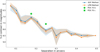Fig. 10 5-σ contrast curve of both the SGF and LPM methods with 50% detection in solid line as well as 25% and 75% delimiting colored areas. Planets PDS70 b and c are also placed at their contrast and separation. Both are detected by both methods.

3.3.3 ROC curves

Alternatively, a common approach to assess the robustness of detection of a binary classifier is to build its receiver operating characteristic (ROC) curve. Thresholding of a detection image (whether it comes from the averaging of monochromatic images of interest or from matched filtering with spatio-spectral models) being a binary classification, it can be evaluated in this way.

The ROC curve of a binary classifier is meant to represent its detection probability (DP) and its false alarm probability (FAP), when the detection threshold varies. Thus, an ideal detector is characterized by both a probability of false alarm equal to 0 and a probability of detection equal to 1. On the contrary, a classifier that leads to DP = FAP is not better than the random classifier accepting or rejecting the detection with the same probability of 0.5. A typical way to assess the performance of such a classifier is to compute the area under the curve (AUC) expressing DP as a function of FAP (Kay 1997). Following what is said just above, the AUC values range from 0.5 (for the random classifier) to 1 (for the perfect classifier). Below, any classifier can be replaced by its inverse classifier for strictly better detection performance.

Another advantage of the ROC curve is that its construction can be experimental, without requiring any assumption on the noise distribution. The FAP can be estimated from real data that may contain buggy pixels, ghosts, or speckles (Réfrégier et al. 2007). Yet, the drawback is that it illustrates only one scenario, for example at a given separation and contrast in our situation. Several bundles of curves for different scenarios (e.g., different separations) can be plotted to overcome this problem.

6 of these curves are shown in Fig. 11 for 2 methods and 3 separations. A general overview of the ROC curves construction method is summarized in Fig. F.1. The same planetary models as for the contrast curves were used (see Sect. 3.3.2). An injection contrast of 1.7 × 10⁻³ was chosen to illustrate a PDS70 b-like scenario, namely, at the detection limit. Injection positions at 3 different separations are chosen: ~0.14″, ~0.25″, and ~0.35″. This ensured that the injected planets were all within the correction radius of the AO without being too close to the star core.

Classification was performed by thresholding the matched filter map of the post-subtraction residuals. The same models as those described in Sect. 3.3.1 were used for matched filtering; thus, the thresholding was performed on values of the output of the normalized matched filter. The FAP and DP were evaluated by applying thresholding chosen to adequately sample the output dynamic of the matched filter (Helstrom 1994). This latter thus varied between −1 and 0.5 in steps of 0.0001 for the construction of these curves. The number of noise realizations was 4 × 310 by injecting the planets into the four cubes at our disposal, and in the 310 spectral channels 1090 to 1399 and 1503 to 1811 by steps of two spectral channels, namely at wavelengths 6112.8 À to 6497.8 À and 6627.8 À to 7012.8 À by steps of 2.5 À (knowing that the H_α line is centered at spectral channel 1451 i.e., at a wavelength of 6562.8 À); the two true planets PDS70 b and c did not influence the detection of the fake planets for either of the two methods in this way. The contrasts were set according to the stellar flux values at the corresponding wavelengths.

For each of the threshold values, the detection probabilities were estimated by the ratio of the number of detected planets (i.e., with fluxes at their positions above the threshold value) to the number of detectable planets (i.e., 4 × 310). Similarly, for each of the threshold values, the false alarm probabilities were estimated by the ratio of the number of false alarms (i.e., where the fluxes are above the threshold, and outside planetary zones) to the total number of potential false alarms (i.e., where the field has been restricted, and outside planetary zones). The planetary zones are positions around the fake planets that are not counted as false alarms because of their fluxes mainly coming from the planets (whose fluxes are spread around by the PSF). For these planetary zones, we chose the 3 × 3 pixels square around the planet positions, which corresponds approximately to the FWHM of the spatial PSF at these injection fluxes.

Finally, while the discussion in Sect. 3.3.2 demonstrates the similarity of the detection capabilities of both methods based on a first detection metric, this section is aimed at showing that the LPM method provides the same detection capabilities as the SGF method (to the given margin of error), this time with respect to robustness (i.e., precision-return trade-off). A slight lack of noise diversity would be deplored for correctly estimating the curve at the regime of interest, i.e., low false alarm probabilities (e.g., FAP < 2.87 × 10⁻⁷ and DP = 0.5 for the construction of a contrast curve). However, it can be assumed that the behavior of the curves with respect to each other remains the same whatever the false alarm regime chosen, especially given the importance of the margin of error (plotted at 1-σ, here, with σ the standard deviation along the four post-subtraction residuals).

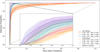Fig. 11 Bundle of ROC curves, for both halo subtraction methods, and for various fake planet injections separations; a zoom for FAP between 0 and 10−2 is included. The random classifier, which validates or invalidates detections with the same probability of 0.5 is shown as a dotted diagonal line for comparison. AUC stands for area under the curve; by definition, the AUC of the random classifier is equal to 0.5. Contrast curves are located on ROC curves at DP = 0.5 (and 0.25 and 0.75 to built error margins as in Fig. 10 for example) and FAP = 2.87 × 10−7 (corresponding to a 5-σ confidence interval). Data is lacking to produce an accurate curve, especially around FAP = 2.87 × 10−7, but this still shows that, within the 1-σ margin of error, the two stellar halo subtraction methods have relatively equivalent overall robustness as well.

3.4 Impact on characterization: The binary system HTLup

We used HTLup observations to explore the potential of both methods in the case of low contrasts, tight pairs (~ 170 mas), and relatively close spectral features between the binary components (the primary is a K3V star while the companion is an M dwarf; see more details below). In this section, we confirm the impact of the signal distortion caused by the SGF method in such an extreme scenario, and how the LPM method alleviates this issue.

After subtracting the stellar halo of each of the selected cubes (see Appendix C) and with each of the two methods, an aperture of 3 x 3 pixels (with the spatial PSF having a ~3 pixels FWHM) was used to integrate the companion flux at every wavelengths. To estimate the losses outside of this aperture, a compensation ratio was calculated from the stellar flux before subtraction, as the ratio of the integration over the entire field to that over only the 3 × 3 pixel aperture. At each wavelength, the total flux was thus finally estimated by integration over the 3 × 3 aperture, each time multiplied by a different compensation ratio, function of the wavelength to account for the spectral dependence of the spatial PSF (leading to the spectral dependence of the losses too).

Finally, the median of the spectra (shown in Fig. 12) obtained with both methods reveals, as expected, two different extracted spectra. Indeed, the high contrast of HTLup B with respect to the noise level leads to critical overfitting with the SGF method, and subsequently to noticeable self-subtraction (also reported in Jorquera et al. 2024). All emission lines revealed with the SGF method by Jorquera et al. (2024) were also recovered by the LPM method, namely the H_α and H_β lines, as well as the CaII infrared triplet. However, unlike the SGF method, the LPM method also partially reconstructed fragments of the continuum fluctuations. Although it is not fully quantifiable in a trustworthy way, it allows us to recognize patterns identifiable as TiO and Na absorptions, while unveiling the absence of others such as VO absorptions; this suggests that HTLup B might be a late-M type star. What is more quantifiable, nonetheless, is the effect of the LPM method on the H _α line compared to the SGF method. Markedly, measurements gave a difference in the integrated flux of ~30%, and differences in velocity at the 10% and 50% of the maximum flux of the line of ~8%; importantly, these measures can be used for deriving accretion rates (the estimation given by the routines built for Jorquera et al. (2024) was improved from 2.4 × 10⁻⁹ M_Sun/year to 3.2 × 10⁻⁹ M_Sun/year in this situation) or discriminating between chromospheric activity and accretion as line emission mechanisms.

To qualify these results, we note that when self-subtraction is noticeable, corrective treatments of the estimates are possible; especially to artificially correct negative fluxes around the lines. For example, in Jorquera et al. (2024), the negative values of the estimated spectrum of HTLup B around the H_α line being obviously non-physical, an estimation of the loss was added to the recovered spectrum prior to any analysis with line models (which cannot deal with negative fluxes). This was done through fake planets injections at the same contrast and separation. Then, the estimated loss was the difference between the line height of the injected planet and the one of the recovered fake planet after stellar halo subtraction. This procedure yielded lines relatively similar to those estimated by the LPM method, leading to less significant physical consequences in practice.

We note that when the lines are too faint compared to the noise level, as for protoplanets PDS70 b and c, only very few changes can be seen between the SGF and the LPM methods. Additionally, in their case, the continuum seems to be too faint to be detected by the LPM method.

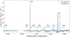Fig. 12 HTLup B spectrum estimates by the SGF (in blue) and LPM (in orange) methods. The Hα, Hβ, and [OI] lines as well as the CaII infrared triplet are detected by the SGF method. Absorptions of TiO and Na are revealed by the LPM method in addition, thanks to its greater preservation of the continuum. On the contrary, it reveals the absence of any VO absorptions, suggesting that the star should be a late-M type. Further improvements of the LPM method are planned to improve the continuum recovery and its quantification (see Sect. 4.2) so that it would be indeed usable for physical interpretations. Yet, a more complex study is beyond the scope of this paper, which is primarily focused on the Hα line (or, similarly, any other emission line).

3.5 Looking for line emission in the YSES1 planetary system

YSES1 observations offer a chance to further validate the new method on the sky. YSES1 b and c are early-L and late-L type objects (Bohn et al. 2020b), with spectral features that diverge from those of their host star YSES1, and with larger separations. We processed every individual data cube of YSES1 with both halo subtraction methods and median-combined the residuals. The YSES1 c companion was not detected at H_α wavelengths (Jorquera et al., in prep.), whose accretion model predicts to be the brightest emission (Aoyama et al. 2020). We focus on the comparison of the YSES1 b spectrum estimates, and in particular on the few emission lines (presented in Figs. 13 and 14). There, the colored areas are delimiting the 1-σ confidence intervals with regard to noise. They were estimated as the root mean square deviation from the mean of the integrated flux on 3 × 3 apertures at different angular positions at the same separation. They were also corrected by the ratio of total flux to 3 × 3 aperture flux.

We detected H_α and H_β lines on YSES1 b (Figs. 13 and 14), as well as HeI lines (at 6678Å and 7065 Å) and the CaII H&K triplet (at 8498 Å, 8542 Å, and 8662Å). YSES1 b is thus the only second object (following Delorme 1 AB b) in this mass range known to display HeI emission lines (Eriksson et al. 2020) and the only object in this mass range to display this full combination of lines. All these lines are usually observed on accreting and/or active stars, but the presence of a circumplanetary disk around the companion advocates for accretion as an origin of the lines.

Figures 13 and 14 reveal the self-subtraction problem caused by the SGF method, as well as its correction by the LPM method. Estimations of the main parameters of the lines were made from Gaussian fitting to compare the results (recorded in the legends). Notably, the H_α and H_β lines exhibit maximum flux differences of ~5% and ~6%, as well as 10% integrated flux differences of ~7% and ~6%. Confidence intervals were determined from Gaussian fitting on the lower and upper bounds of the ones of the spectra. Using the routines built for Jorquera et al. (2024), we derived, for the SGF and LPM methods, accretion rates of $1.11\times {10}^{-9\pm 0.19}{\mathrm{M}}_{\mathrm{J}\mathrm{u}\mathrm{p}}/\mathrm{y}\mathrm{e}\mathrm{a}\mathrm{r}$ and $1.45\times {10}^{-9\pm 0.19}{\mathrm{M}}_{\mathrm{J}\mathrm{u}\mathrm{p}}/\mathrm{y}\mathrm{e}\mathrm{a}\mathrm{r}$ from the H_α line flux (the errors are systematic errors derived from model fits by the routines). Thus, we found the SGF method underestimates the accretion rates by ~30%. The accretion rate is comparable to those of objects of similar masses (Betti et al. 2023). A follow-up study, focused on the characterization of the accretion mechanisms on YSES1 b using these observations and complementary data, is in progress (Jorquera et al., in prep.).

To go even further, we injected fake planets into all YSES1 cubes (following Appendix E) and performed both stellar halo subtraction methods. The results are presented in Appendix D.

Qualitatively and quantitatively, with MSE calculation for the line and for the continuum, they confirm all the self-subtraction issues and corrections highlighted in this paper.

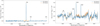Fig. 13 YSES1 b spectrum estimates, by the SGF (in blue) and LPM (in orange) methods. Left: zoom in on 821 channels around the Hα line. The self-subtraction caused by the SGF method as well as its correction by the proposed LPM method are visible. Two HeI lines are also revealed. Right: zoom in on 821 channels around the CaII infrared triplet. The self-subtraction around the lines is less visible here, because both the lines are weaker and the continuum is (likely) stronger at these wavelengths (yet, in turn, the heights of the lines are theoretically further underestimated); the mask used by the LPM method during this estimation process was adapted to cover the full triplet. A noticeable Na absorption is also revealed.

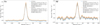Fig. 14 Zoom in on 51 channels around the Hα (left) and Hβ (right) lines of the YSES1 b spectrum estimates, from stellar halo subtraction, both with the SGF (in blue) and LPM (in orange) methods. The horizontal dots indicate the zero-flux level, i.e., the theoretical flux lower bound. Colored areas delimit the 1-σ confidence intervals with regard to noise. Dotted Gaussians are fitted to the lines to estimate their main parameters (presented in the legend, with confidence intervals derived from Gaussian fits to the lower and upper bounds of those of the spectrum estimates).

4 Concluding remarks

4.1 Remaining limitations of the LPM method

An interesting take on the LPM method is that estimating the stellar component via an orthogonal projection of the data on the vector space of the modulation matrix, while estimating the planetary component via the subtraction of this stellar estimate, is equivalent to the orthogonal decomposition of the data. This means that the subtraction quality depends on the orthogonality of the stellar and planetary spectra vectors.

The proposed LPM method is thus optimal for extracting companions with spectra orthogonal to the one of their host star, and, on the contrary, blind to every companions with spectra collinear with the one of their host star. Assuming positive values for the spectra, the angle between two spectra is close to ± π/2 when, for given total fluxes, their inner product is close to 0. Thus, assuming a stellar spectrum dominated by the continuum, our proposed method is particularly adapted for detecting and characterizing companions with sparse spectra (e.g., either with accretion or chromospheric activity producing emission lines). On the contrary, the approach is still limited when the stellar spaxel and the planetary spaxel have identical flux ratios over the entire wavelength (or, as shown in Fig. 5, more realistically, when they exhibit a similarity up to a certain factor).

We quantified this behavior via the calculations presented in Appendix B.3, looking for the best possible planetary estimate when the stellar component is perfectly estimated. This gives both a relative angle and an upper bound on the norms ratio.

4.2 Discussions

The primary aim of this article is to lay the foundations for a new halo subtraction method which can be complemented by other advanced signal processing techniques to improve both the detection and the characterization of accreting companions.

Whether in the case of simulations or real data observations, the LPM and SGF methods have similar detection capabilities.

Regarding characterization, however, a comparative analysis of the H_α line estimates, from the two halo subtraction methods, indicates that the accretion rate was underestimated by ~30% (2.4 x 10⁻⁹ M_Sun/year instead of 3.2 × 10⁻⁹ M_Sun/year), in the case of the low-mass stellar accreting companion HTLup B. In contrast, no significant change could be noticed regarding the fainter PDS 70 b and c; consequently, tour conclusions on the interpretations of the lines remain unchanged (Aoyama & Ikoma 2019; Thanathibodee et al. 2019; Hashimoto et al. 2020). Yet, for the intermediate YSES1 b case, changes were revealed by the LPM method as well, indicating that the accretion rate was underestimated by ~30% when using the SGF method (1.11 x 10⁻⁹ M_Jup/year instead of 1.45 × 10⁻⁹ M_Jup/year).

In fact, self-subtraction not only disrupts subsequent routines with unexpected negative flux values, but also vertically distorts the lines so that, whatever is attempted, it becomes impossible to recover their actual parameters: information is truly lost.

Importantly, the improvements offered by the LPM method are applicable to other techniques derived from the SGF method, such as molecular mapping (see Sect. 1). The lack of filtering at the stellar halo subtraction step guarantees that information on the molecular lines of cool companions is preserved; in turn, this could secure the estimate of their molecular abundances and rotation velocities (e.g., Petrus et al. 2021).

And finally, even more importantly, our proposed approach moves from a non-linear and non-parametric model of the data to a linear and parametric one. This offers to use more advanced machine learning approaches and signal processing techniques. Future refinements of the method could include weighting of the estimates by precision matrices based on covariance matrices to improve robustness to noise and defaults. Better local estimates of the stellar spectrum would now also be usable to deal with the various instrumental defaults. Ultimately, spatial and spectral regularization (in a greedy approach) would allow us to recover planetary continua and absorptions. This would be a new source of information to that provided by the lines, opening up brand new research directions, both in signal processing, from inverse problems to faint signal search algorithms, and in astrophysics, from molecular mapping to planet formation processes.

Acknowledgements

We acknowledge support from the French National Research Agency (ANR) through project grant ANR-20-CE31-0012 and the Programmes Nationaux de Planétologie et de Physique Stellaire (PNP and PNPS). We thank Maud Langlois and Eric Thiébaut for fruitful discussions about mathematical modeling of the problem and its solution. We thank Chen Xie, Jun Hashimoto, and Sebastiaan Haffert for fruitful discussions about the data analysis and for sending their data cubes for comparison. S.J. acknowledges support from the National Agency for Research and Development (ANID), Scholarship Program, Doctorado Becas Nacionales/2020 - 21212356. We thank the anonymous referee for her/his careful reading of the manuscript as well as her/his insightful comments and suggestions.

References

Appendix A Stellar halo subtraction methods

Appendix A.1 Model of the observations

Let $\mathcal{A}\in {\mathbb{R}}^{\ell \times m\times n}$ stands for the ideal theoretical hyperspectral data cube, with ℓ spectral channels, m pixels in the horizontal direction, and n pixels in the vertical direction. For $i\in [\ell$², the monochromatic image at wavelength λ_i is defined by the matrix A_i ∈ R^m×n of the elements of A along the second and third axes. For (x, y) ∈ [m] × [n], the spaxel at position (x, y) is defined by the vector ${\mathit{a}}_{xy}\in {\mathbb{R}}^{\ell }$ of the elements of A along the first axis. Following these notations, the ideal data cube containing u unresolved astronomical bodies at positions (x_j, y_j) for j ∈ [u] is: $$\mathcal{A}=\sum _{j=1}^u{\stackrel{\mathbf{ˇ}}{\mathit{a}}}^{(j)}\otimes {\mathbf{\Delta }}^{(j)},$$(A.1)

where ⊗ stands for the outer product (e.g., here, between a vector and a matrix representing a spaxel and a monochromatic image). The matrix ${\mathbf{\Delta }}^{(j)}\in {\mathbb{R}}^{m\times n}$ satisfies ${\mathbf{\Delta }}^{(j)}=\delta (x-x_j)\delta (y-y_j)$ and equals 1 at position (x_j,y_j and 0 otherwise. It indicates the position of the j^th object for which the vector ${\stackrel{\mathbf{ˇ}}{\mathit{a}}}^{(j)}\in {\mathbb{R}}^{\ell }$ is the ideal spectrum. The use of ${\mathbf{\Delta }}^{(j)}$ comes from the assumption that the observed objects (typically a host star and several accreting companions in the context of this article) are unresolved by the optical system and thus appear as point sources (which seems reasonable in the case of images from the MUSE instrument, each of its pixels covering an area of 0.025 × 0.025” and thus, typically at a distance of 100 pc, receiving the flux of 2.5 x 2.5AU area in the sky - note also that the chances of an object straddling two pixels are consequently very low under these conditions).

For an actual imaging system (assumed linear), we introduce the observed data cube noted O: $$\mathcal{O}=\mathcal{A}\ast \mathbf{\Omega },$$(A.2)

where * stands for the Fredholm operator. The 6-dimensional tensor $\mathbf{\Omega }\in {\mathbb{R}}^{(\ell \times m\times n)\times (\ell \times m\times n)}$ is the tensor of the 3-dimensional point spread function (PSF) of the optical system (IFS, telescope, AO, atmosphere). Its effect is to spread the flux $a_{i^{\prime }{x}^{\prime }{y}^{\prime }}$ of each pixel of position (x′, y′) and wavelength λ_i of A on each pixel of position (x, y) and wavelength λ_i of O: $$\mathcal{O}=\sum _{i^{\prime }=1}^{\ell }\sum _{x^{\prime }=1}^m\sum _{y^{\prime }=1}^n{a}_{i^{\prime }{x}^{\prime }{y}^{\prime }}{\mathbf{\Omega }}_{i^{\prime }{x}^{\prime }{y}^{\prime }:::},$$(A.3)

where ${\mathbf{\Omega }}_{i^{\prime }{x}^{\prime }{y}^{\prime }:::}$ is the 3-dimensional response of the total system at position (x′, y′) and wavelength λ_i′. Conversely, each element o_ixy of O is the sum of each of the flux contributions $a_{i^{\prime }{x}^{\prime }{y}^{\prime }}$ of A, more or less spread out from their initial spatio-spectral position.

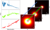Fig. A.1 Spatio-spectral simulation of a star observation. On the right, three monochromatic images are shown at wavelengths λ1, λ1841, λ3681 to highlight the spatial spread variation with wavelength. On the left, three spaxels are shown at three different separations to highlight the spectrum deformation caused by this spatial spread variation.

For convenience, this 3D point spread function, ${\mathbf{\Omega }}_{i^{\prime }{x}^{\prime }{y}^{\prime }:::}$, is commonly spatio-spectrally separated into a 1D spectral PSF (known as the LSF for line spread function) and a 2D spatial PSF (known as the FSF for field spread function), both wavelength dependent. The spatial dependence is neglected using the small-field hypothesis, whose use is relevant here by reducing the study to the AO correction radius (note however that the PSF could spatially vary in some integral field spectrograph images due to imperfect calibration of the cubes, instrument flexure or even scattered light, as shown for example in Xie et al. 2020). This results in the PSF expression at wavelength λ_i : $${\text{PSF}}_{i^{\prime }}(i,x,y)={\text{LSF}}_{i^{\prime }}(i)\times {\text{FSF}}_{i^{\prime }}(x,y),$$(A.4)

We note that for each pixel, this means neglecting all the flux scattered towards or from pixels both at neighboring positions and at neighboring wavelengths (i.e. along the cube’s diagonals).

The presence of this PSF induces a spread on the spectral axis at each position (x, y) and a spread in the image plane at each wavelength λ_i. The integration of the PSF over the whole field and over the spectral direction is set to 1 to satisfy the flux conservation constraint. The separation assumption of Eq. (A.4) implies that this flux constraint must also be satisfied separately for both the LSF and the FSF.

Consequently, in practice, only spectrally spread versions of the spectra ${\mathit{a}}^{(j)}={\stackrel{\mathbf{ˇ}}{\mathit{a}}}^{(j)}\ast \mathit{\psi }$ are observed, the matrix $\mathit{\psi }\in {\mathbb{R}}^{\ell \times \ell }$ containing LSF information for each spectral channel of index i and thus expressing the wavelength dependency of the spectral spread with the Fredholm operator. As the LSF is little known and the spectra are (very) noisy, it is usual to settle for these imperfect spectrally spread spectra, a^(j), rather than attempt their spectral deconvolution (the models being convolved with an LSF approximation instead).

Similarly, these are u spreads ${\mathit{\varphi }}_i^{(j)}={\mathit{\varphi }}_i\ast {\mathbf{\Delta }}^{(j)}$ on each of the monochromatic images at wavelength λ_i that are observed at positions $(x_j,y_j)$, the matrix ${\mathit{\varphi }}_i\in {\mathbb{R}}^{m\times n}$ expressing the spectral dependency of the spatial spread with the Fredholm operator by containing FSF information for each spectral channel of index i.

The separation assumption of Eq. (A.4) allows us to express the observed image at wavelength λ_i as: $${\mathit{O}}_i=\sum _{j=1}^u{a}_i^{(j)}{\mathit{\varphi }}_i^{(j)},\mathrm{\forall }i\in [\ell ],$$(A.5)

where the scalar $a_i^{(j)}\in \mathbb{R}$ is the flux observed from the j^th object at wavelength λ_i and is given by the i^th entry of the vector a^(j). Because of the PSF normalization, $a_i^{(1)}$ is the total integrated flux of the image O_i when a single unresolved object is observed.

However, it is difficult to deal with the FSF for postprocessing operations because of its complex shape, notably due to the atmospheric turbulence effects and AO system corrections. We thus seek to reverse its effect in the spectral direction in which it is expected to behave more simply. For this purpose, we define the chromatic spread function (CSF), a chromatic PSF in a way. Its associated vector is determined from the FSF tensor $\mathbf{\Phi }={\left({\mathit{\varphi }}_i\right)}_{i\in [\ell ]}\in {\mathbb{R}}^{\ell \times m\times n}$, constructed from the FSF matrices at each of the observed wavelengths. Whereas the set of the FSF matrices corresponds to the ℓ two-dimensional spatial entries of this tensor, the set of the CSF vectors corresponds to the m × n one-dimensional spectral entries of this tensor. We note ${\mathit{\alpha }}_{xy}\in {\mathbb{R}}^{\ell }$ for these vectors at each position (x, y) ∈ [m] × [n].

As illustrated by Fig. A.1, the α_xy can be understood as a set of deformation coefficients, which allows us to explicit all the expressions of the spaxels from objects’ spectra. By defining the vectors ${\mathit{\alpha }}_{xy}^{(j)}$ as above, for $j\in [u]$, from the tensors Φ^(j) built with the set of the ${\mathit{\varphi }}_i^{(j)}$ matrices, the spaxels of the observation cube can be written as spectra a^(j) deformed by coefficients ${\mathit{\alpha }}_{xy}^{(j)}$: $${\mathit{o}}_{xy}=\sum _{j=1}^u{\mathit{a}}^{(j)}\cdot {\mathit{\alpha }}_{xy}^{(j)},\mathrm{\forall }(x,y)\in [m]\times [n],$$(A.6)

where ∙ stands for the Hadamard (entrywise) product.

More specifically, the studied observations show two types of unresolved astronomical bodies. To illustrate this duality, the observation cube is decomposed as O = S + P with P a signal cube associated to u_P  0 unresolved sources (typically from protoplanets or other accreting companions like young stars) and S a nuisance cube (typically from one bright star). Both take into account the spatio-spectral deformations previously described.

Finally, in addition to all the optical effects described above, the cubes are also affected by various noise sources (read-out, thermal fluctuations, and photon noises). Although they follow various probability laws, these noises are (relatively) realistically encompassed in a centered, symmetrically distributed Gaussian noise (see Appendix G for additional details on this assumption). We let E denote the cube whose elements contain the random noise realizations that are assumed to be additive. Furthermore, for the sake of simplicity, these realizations are assumed to be spatially independent and identically distributed (although this amounts to ignoring the correlation between nearby pixels).

Then, the expression of the data, D, that we consider for this entire study can be expressed by the sum of three components: $$\mathcal{D}=\mathcal{S}+\mathcal{P}+\mathcal{E}.$$(A.7)

The values of the noise component, E, being assumed centered, it can be mitigated by multiple approaches: median of various exposures, sigma-clipping, or even matched filtering (proposed in Sect. 3.3.1). A low-noise framework is thus considered for the theoretical problem solving described below, where S and P are the dominant contributions.

Appendix A.2 Problem statement

The planetary signal estimate, P, is determined by subtraction from the data, D, of an estimate, S, of the stellar nuisance: $$\hat{\mathcal{P}}=\mathcal{D}-\hat{\mathcal{S}}.$$(A.8)

This is the so-called “stellar halo subtraction,” a classic method for detecting planets masked by the halo of their star in direct imaging. This technique has many variants, notably depending on how the stellar component is estimated (e.g., from temporal diversity (Marois et al. 2005) or from spectral diversity (Hoeijmakers et al. 2018). Both solutions described in the following are based on the spectral diversity, the stellar nuisance estimate being based on the data model of Eq. (A.6). The deformation, α_xy, is assumed to be smooth (although more complex in the case of VLT/MUSE or VLT/SINFONI observations than in the case of diffraction limited observations because of the system of AO notably providing higher Strehl at the longest wavelengths), allowing for its estimation by simple models. A spaxel-by-spaxel estimation of the stellar nuisance contribution (i.e., without any spatial a priori) is enabled by this approach.

We let s_xy be the stellar nuisance contribution to the data spaxel at position (x, y), and ${\hat{\mathit{s}}}_{xy}$ its estimation. According to the CSF-based model of the observations given by Eq. (A.6), s_xy = s ∙ α_xy, where s stands for the stellar nuisance spectrum (distorted by the LSF). The estimation problem can thus come down to determining both $\hat{\mathit{s}}$ the estimate of s for the whole field and â_xy the estimate of α_xy at each position (x, y) : $${\hat{\mathit{s}}}_{xy}=\hat{\mathit{s}}\cdot {\hat{\mathit{\alpha }}}_{xy}.$$(A.9)

As it is assumed that the optical system preserves the total flux (all φ_i sum to 1), s is nothing more than the integrated flux over the field in the absence of planet and noise. The random noise being centered, and a potential planet being faint, the integration of the flux over the field at each spectral channel is already a good estimate s of s (the weight of the planetary contribution to this integrated flux being expected to be weak). In practice, the spaxels from the edges of the field are masked because the stellar signal is too low there to be reliable. Similarly, in practice, the spaxels around the star center are masked because more likely to be considered as outliers by the MUSE pipeline and, therefore, replaced by too rough approximations interpolating neighboring values (in particular when the Strehl ratio is high). The integrated flux thus no longer matches the total flux of the star, but this does not rule out the usefulness of Eq. (A.9). Indeed, estimating both s and α_xy jointly can only be done up to a multiplicative indeterminacy (at the cost of losing the flux conservation). Thus, for the same reasons, this sum can even be replaced by a mean (this only changes the estimate by the factor m × n) and therefore also by a median for increased robustness.

Although much remains to be done to improve the estimate s of the stellar spectrum, s, this article focuses on the improvement of the estimate ${\hat{\mathit{\alpha }}}_{xy}$ of the deformation coefficients, α_xy.

Appendix A.3 State-of-the-art solution

While Keppler et al. (2018) reported the first detection of a protoplanet (a.k.a. PDS70 b) using classical detection techniques (i.e., angular/polarimetric differential imaging with VLT/SPHERE, VLT/NaCo, and Gemini/NICI instruments), Haffert et al. (2019) used a spaxel-by-spaxel approach adapted from Hoeijmakers et al. (2018) for the first detection of the second known protoplanet (a.k.a. PDS70 c, in the same system). The principle of the method, which we refer to as the Savitzky-Golay filtering (SGF) method, is sketched in Fig. A.2. It can also be expressed using the quantities ${\hat{\mathit{\alpha }}}_{xy}$, d_xy, and s described in the previous section. The following equation sums up the process of estimation of the geometric deformation in this case: $${\hat{\mathit{\alpha }}}_{xy}=\text{SG}({\mathit{d}}_{xy}./\hat{\mathit{s}}),$$(A.10)

where the rationale consists in inverting Eq. (A.9) using the Hadamard (entrywise) division ./. The spaxel d_xy can be seen as a rough estimate of the unknown stellar component spaxel, s_xy, at position (x, y). The low-pass filtering (by a Savitzky-Golay filter of degree d and spectral window size AW) aims at removing high frequencies of p_xy to derive a smooth estimate α_xy of α_xy.

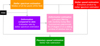Fig. A.2 General principle of the SGF stellar halo subtraction method presented in Haffert et al. (2019). Each planetary spaxel (in green) is estimated by subtraction from the data (in black) of an estimate of the stellar spaxel (in red). This latter is estimated by entrywise product of the stellar spectrum estimate (in orange) by the deformation coefficient estimate (in pink). This estimate is made by low-pass filtering of the stellar spectrum estimate to data spaxel ratio (in purple).

Appendix A.4 Our proposed solution

To tackle the problem of self-subtraction and spectral distortion, we propose to estimate ${\hat{\mathit{\alpha }}}_{xy}$ as a smooth function of the wavelengths, λ_i, expressed as a polynomial function of degree ∂: $${\hat{\mathit{\alpha }}}_{xy}={\left(\sum _{k=0}^{\mathrm{\partial }}{\lambda }_i^k{\hat{\beta }}_{xyk}\right)}_{i\in [\ell ]},$$(A.11)

where ${\hat{\beta }}_{xyk}$ is the k^th regression coefficient at position (x,y). Equivalently (using Eq. (A.9)), the stellar spaxels estimates, ${\hat{\mathit{s}}}_{xy}$, are modeled as polynomial modulations of degree ∂ of the stellar spectrum estimate, s: $${\hat{\mathit{s}}}_{xy}={\left(\sum _{k=0}^{\mathrm{\partial }}{\lambda }_i^k{\hat{\beta }}_{xyk}{\hat{s}}_i\right)}_{i\in [\ell ]}.$$(A.12)

The complexity of the learning model is driven by an only hyperparameter: the degree of the polynomial model, ∂. Its value must be chosen wisely for a good stellar nuisance estimate. Moreover, this linear regression model can be written in a matrix form as: $${\mathit{s}}_{xy}=\mathit{M}{\mathit{\beta }}_{xy}+{\mathit{\epsilon }}_{xy},$$(A.13)

where $\mathit{M}\in {\mathbb{R}}^{\ell \times \mathrm{\partial }+1}$ is the design matrix defined for $k\in [[\mathrm{\partial }]]$³ by columns ${\mathit{m}}_k={\mathit{\lambda }}^{\cdot k}\cdot \hat{\mathit{s}}\in {\mathbb{R}}^{\ell },{\mathit{\lambda }}^{\cdot k}=({\lambda }_1^k,\dots ,{\lambda }_{\ell }^k)$. The column space of M is the set of polynomial modulations of the stellar spectrum estimate. The vector β_xy is the vector of the unknown regression coefficients, defined as ${\mathit{\beta }}_{xy}={\left({\beta }_{xyk}\right)}_{k\in [[\mathrm{\partial }]]}\in {\mathbb{R}}^{\mathrm{\partial }+1}$ and estimated by ordinary least squares: $${\hat{\mathit{\beta }}}_{xy}=\underset{\mathit{\beta }}{\mathrm{a}\mathrm{r}\mathrm{g}\mathrm{m}\mathrm{i}\mathrm{n}}||{\mathit{d}}_{xy}-\mathit{M}\mathit{\beta }|{|}_2^2=({\mathit{M}}^{\mathrm{\top }}\mathit{M}{)}^{-1}{\mathit{M}}^{\mathrm{\top }}{\mathit{d}}_{xy}.$$(A.14)

Fig. A.3 General principle of the LPM stellar halo subtraction method we propose. Each planetary spaxel (in green) is estimated by subtraction from the data (in black) of an estimate of the stellar spaxel (in red). This latter is estimated by polynomial modulation (in pink) of the stellar spectrum estimate (in orange). In practice, this is done by multiplication of the data spaxel by the orthogonal projection matrix onto the column space of the design matrix of the polynomial modulation (in brown).

By defining ${\mathbf{\Pi }}_{\mathit{M}}=\mathit{M}({\mathit{M}}^{\mathrm{\top }}\mathit{M}{)}^{-1}{\mathit{M}}^{\mathrm{\top }}$ the orthogonal projection matrix onto the column space of M, the expression of the stellar nuisance estimate finally reduces to: $${\hat{\mathit{s}}}_{xy}={\mathbf{\Pi }}_{\mathit{M}}{\mathit{d}}_{xy}.$$(A.15)

The whole estimation process is summarized in Fig. A.3 and named the Legendre polynomial modulation (LPM) method.

Indeed, it is well-known that the Gram matrix M^T M is badly conditioned when using the canonical monomial basis (Seber & Lee 2012). Thus, we proposed to expand the data spaxel, d_xy, on an orthogonal basis, with Legendre polynomials. More details are provided in Julo et al. (2024). This change in the basis has the major advantage, in addition, of restoring physical interpretation of the d + 1 coefficients of the estimation polynomials, as in this way each of them explains different FSF components at different spectral frequencies (see Fig. 7 for a real FSF decomposition).

Appendix B Analytical calculations

Appendix B.1 Low-pass filtering effect with the SGF method

We study in this section the effect of a first-order Savitzky-Golay filtering of window width 2w_max + 1 on a simple flat signal with a single peak of width 2w_peak + 1, base h_min and height h_max — h_min. In particular, for the window centered on the peak, the linear regression is performed on the following signal, represented as two sets accounting for abscissa and ordinate, respectively: $$\mathrm{L}={\left(l_w\right)}_{w\in W}\text{\hspace{0.17em}and\hspace{0.17em}}\mathrm{H}={\left(h_w\right)}_{w\in W}\text{\hspace{0.17em}for\hspace{0.17em}}W=[-w_{\mathrm{m}\mathrm{a}\mathrm{x}},w_{\mathrm{m}\mathrm{a}\mathrm{x}}].$$

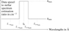Fig. B.1 Simple peak model sampled in wavelengths and deformations.

More specifically, assuming that the abscissa axis is regularly sampled at step l_step and that the peak center is correctly sampled at abscissa l_peak, we are now interested in the signal following the simple constraints below (and depicted in Fig. B.1): $$\begin{array}{r}{l}_w=l_{\mathrm{p}\mathrm{e}\mathrm{a}\mathrm{k}}+w{l}_{\mathrm{s}\mathrm{t}\mathrm{e}\mathrm{p}}\text{\hspace{0.17em}and\hspace{0.17em}}{h}_w=\{\begin{array}{l}{h}_{\mathrm{m}\mathrm{a}\mathrm{x}}\text{\hspace{0.17em}if\hspace{0.17em}}w\in [-w_{\mathrm{p}\mathrm{e}\mathrm{a}\mathrm{k}},w_{\mathrm{p}\mathrm{e}\mathrm{a}\mathrm{k}}]\\ h_{\mathrm{m}\mathrm{i}\mathrm{n}}\text{\hspace{0.17em}for all the other points}\end{array}.\end{array}$$

Linear regression with the ordinary least squares method then consists in determining $(b_0,b_1)\in {\mathbb{R}}^2$ minimizing $$\begin{array}{r}\sum _{i=-w_{\mathrm{m}\mathrm{a}\mathrm{x}}}^{i=+w_{\mathrm{m}\mathrm{a}\mathrm{x}}}(h_i-g_i{)}^2\text{\hspace{0.17em}with\hspace{0.17em}}{g}_i=b_0+b_1{l}_i.\end{array}$$

It is known that the solution to this problem is $$\begin{array}{r}\{\begin{array}{l}{b}_1=\mathrm{C}\mathrm{o}\mathrm{v}(\mathrm{L},\mathrm{H})/\mathrm{V}\mathrm{a}\mathrm{r}(\mathrm{L})\\ b_0=\mathrm{M}\mathrm{e}\mathrm{a}\mathrm{n}(\mathrm{H})-b_1\mathrm{M}\mathrm{e}\mathrm{a}\mathrm{n}(\mathrm{L})\end{array},\end{array}$$

with

Mean(L) = l_peak,

and $$\begin{array}{r}\mathrm{M}\mathrm{e}\mathrm{a}\mathrm{n}(\mathrm{H})=\frac{(2w_{\mathrm{p}\mathrm{e}\mathrm{a}\mathrm{k}}+1)h_{\mathrm{m}\mathrm{a}\mathrm{x}}+2(w_{\mathrm{m}\mathrm{a}\mathrm{x}}-w_{\mathrm{p}\mathrm{e}\mathrm{a}\mathrm{k}})h_{\mathrm{m}\mathrm{i}\mathrm{n}}}{2w_{\mathrm{m}\mathrm{a}\mathrm{x}}+1},\end{array}$$

as well as $$\begin{array}{r}\mathrm{V}\mathrm{a}\mathrm{r}(\mathrm{L})=\frac{1}{3}{w}_{\mathrm{m}\mathrm{a}\mathrm{x}}(w_{\mathrm{m}\mathrm{a}\mathrm{x}}+1)l_{\text{step}}^2,\end{array}$$

and $$\begin{array}{r}\mathrm{C}\mathrm{o}\mathrm{v}(\mathrm{L},\mathrm{H})=\frac{2w_w(w_{\mathrm{m}\mathrm{a}\mathrm{x}}+1)(w_{\mathrm{m}\mathrm{a}\mathrm{x}}-w_{\mathrm{p}\mathrm{e}\mathrm{a}\mathrm{k}})}{2w_{\mathrm{m}\mathrm{a}\mathrm{x}}+1}(h_{\mathrm{m}\mathrm{a}\mathrm{x}}+h_{\mathrm{m}\mathrm{i}\mathrm{n}})l_{\text{step}},\end{array}$$

following straightforward computations and leading to $$\begin{array}{r}{b}_1=\frac{6(w_{\mathrm{m}\mathrm{a}\mathrm{x}}-w_{\mathrm{p}\mathrm{e}\mathrm{a}\mathrm{k}})(h_{\mathrm{m}\mathrm{a}\mathrm{x}}+h_{\mathrm{m}\mathrm{i}\mathrm{n}})}{(2w_{\mathrm{m}\mathrm{a}\mathrm{x}}+1)l_{\text{step}}},\end{array}$$

and $$\begin{array}{rl}{b}_0& =\frac{(2w_{\mathrm{p}\mathrm{e}\mathrm{a}\mathrm{k}}+1)h_{\mathrm{m}\mathrm{a}\mathrm{x}}+2(w_{\mathrm{m}\mathrm{a}\mathrm{x}}-w_{\mathrm{p}\mathrm{e}\mathrm{a}\mathrm{k}})h_{\mathrm{m}\mathrm{i}\mathrm{n}}}{2w_{\mathrm{m}\mathrm{a}\mathrm{x}}+1}-b_1{l}_{\mathrm{p}\mathrm{e}\mathrm{a}\mathrm{k}}.\end{array}$$

In particular, the new value returned by the Savitzky-Golay algorithm at the peak abscissa is given by $$g_{\mathrm{p}\mathrm{e}\mathrm{a}\mathrm{k}}=h_{\mathrm{m}\mathrm{i}\mathrm{n}}+\frac{2w_{\mathrm{p}\mathrm{e}\mathrm{a}\mathrm{k}}+1}{\phantom{.}2w_{\mathrm{m}\mathrm{a}\mathrm{x}}+1}(h_{\mathrm{m}\mathrm{a}\mathrm{x}}-h_{\mathrm{m}\mathrm{i}\mathrm{n}}).$$

This expression can be simplified as follows: $$g_{\mathrm{p}\mathrm{e}\mathrm{a}\mathrm{k}}=\mathrm{H}+\mathrm{R}\overline{\mathrm{H}},$$

with

• $\mathrm{H}={\mathrm{h}}_{\mathrm{m}\mathrm{i}\mathrm{n}}$ the base of the peak,

• $\mathrm{R}=\frac{2w_{\mathrm{p}\mathrm{e}\mathrm{a}\mathrm{k}}+1}{\phantom{.}2w_{\mathrm{m}\mathrm{a}\mathrm{x}}+1}$ the ratio of the peak to window widths,

• $\overline{\mathrm{H}}=h_{\mathrm{m}\mathrm{a}\mathrm{x}}-h_{\mathrm{m}\mathrm{i}\mathrm{n}}$ the height of the peak relative to its base.

Appendix B.2 Residual distribution with the LPM method

Appendix B.2.1 Analytic expression of the spaxels estimates

The use of the orthogonal projection matrix, Π_m, allows us to identify the contribution of each of the components of the data in the stellar spectrum estimate (using Eq. (A.7) and (A.9)): $${\hat{\mathit{s}}}_{xy}={\mathbf{\Pi }}_{\mathit{M}}{\mathit{s}}_{xy}+{\mathbf{\Pi }}_{\mathit{M}}{\mathit{p}}_{xy}+{\mathbf{\Pi }}_{\mathit{M}}{\mathit{e}}_{xy}.$$(B.1)

Indeed, the components of the true stellar spaxel, s_xy, that are orthogonal to the modulation of the stellar spectrum estimate, s, cannot contribute to the stellar spaxel estimate, s_xy. Conversely, the components of the planetary and noise spaxels, p_xy and e_xy, that can be (over)fitted by the modulation model can contribute to the stellar spaxel estimate, ${\hat{\mathit{s}}}_{xy}$.

In the same way, it is possible to identify the contribution of each of the components of the data in the post-subtraction residuals (using the Eq. (A.8)): $${\hat{\mathit{p}}}_{xy}={\mathbf{\Pi }}_{\mathit{M}}^{\perp }{\mathit{s}}_{xy}+{\mathbf{\Pi }}_{\mathit{M}}^{\perp }{\mathit{p}}_{xy}+{\mathbf{\Pi }}_{\mathit{M}}^{\perp }{\mathit{e}}_{xy},$$(B.2)

where the matrix ${\mathbf{\Pi }}_{\mathit{M}}^{\perp }={\mathbf{I}}_{\ell }-{\mathbf{\Pi }}_{\mathit{M}}$ is the matrix of the projection onto the orthogonal complement of the column space of M.

To go a step further, assuming the noise components, e_ixy, to be Gaussian, distributed with standard deviation σ, as well as independent and identically distributed, the distribution of each of the residuals spaxels, ${\hat{\mathit{p}}}_{xy}$, is given by: $${\hat{\mathit{p}}}_{xy}\sim \mathcal{N}({\mathbf{\Pi }}_{\mathit{M}}^{\perp }{\mathit{s}}_{xy}+{\mathbf{\Pi }}_{\mathit{M}}^{\perp }{\mathit{p}}_{xy},{\sigma }^2{\mathbf{\Pi }}_{\mathit{M}}^{\perp }).$$(B.3)

These results are used in Sect. 3.2.1 to select an optimal degree of polynomial modulation, ∂, on simulated datasets, expecting the generalization of the performances to the real data case.

Appendix B.2.2 Decomposition of the Mean Square Error

The mean square error (MSE) defined by: $$\text{MSE}=\mathbb{E}\left({\Vert {\hat{\mathit{p}}}_{xy}-{\mathit{p}}_{xy}\Vert }_2^2\right),$$(B.4)

can be decomposed by expectation linearity using the analytical expression of the planetary component estimation (Eq. (B.2)): $$\text{MSE}={\Vert {\mathbf{\Pi }}_{\mathit{M}}^{\perp }{\mathit{s}}_{xy}\Vert }_2^2+{\Vert {\mathbf{\Pi }}_{\mathit{M}}{\mathit{p}}_{xy}\Vert }_2^2+(\ell -(\mathrm{\partial }+1)){\sigma }^2,$$(B.5)

as the square error (SE) is decomposable as follows: $$\begin{array}{r}\text{SE}={\Vert {\hat{\mathit{p}}}_{xy}-{\mathit{p}}_{xy}\Vert }_2^2={\Vert {\mathbf{\Pi }}_{\mathit{M}}^{\perp }{\mathit{s}}_{xy}+{\mathbf{\Pi }}_{\mathit{M}}^{\perp }{\mathit{p}}_{xy}+{\mathbf{\Pi }}_{\mathit{M}}^{\perp }{\mathit{e}}_{xy}-{\mathit{p}}_{xy}\Vert }_2^2\\ ={\Vert {\mathbf{\Pi }}_{\mathit{M}}^{\perp }({\mathit{s}}_{xy}+{\mathit{e}}_{xy})+{\mathbf{\Pi }}_{\mathit{M}}{\mathit{p}}_{xy}\Vert }_2^2={\Vert {\mathbf{\Pi }}_{\mathit{M}}^{\perp }({\mathit{s}}_{xy}+{\mathit{e}}_{xy})\Vert }_2^2+{\Vert {\mathbf{\Pi }}_{\mathit{M}}{\mathit{p}}_{xy}\Vert }_2^2\\ ={\Vert {\mathbf{\Pi }}_{\mathit{M}}^{\perp }{\mathit{s}}_{xy}\Vert }_2^2+{\Vert {\mathbf{\Pi }}_{\mathit{M}}^{\perp }{\mathit{e}}_{xy}\Vert }_2^2+2{\left({\mathbf{\Pi }}_{\mathit{M}}^{\perp }{\mathit{s}}_{xy}\right)}^{\mathrm{\top }}\left({\mathbf{\Pi }}_{\mathit{M}}^{\perp }{\mathit{e}}_{xy}\right)+{\Vert {\mathbf{\Pi }}_{\mathit{M}}{\mathit{p}}_{xy}\Vert }_2^2,\end{array}$$ $$\text{with}\{\begin{array}{l}\mathbb{E}\left({\Vert {\mathbf{\Pi }}_{\mathit{M}}^{\perp }{\mathit{s}}_{xy}\Vert }_2^2\right)={\Vert {\mathbf{\Pi }}_{\mathit{M}}^{\perp }{\mathit{s}}_{xy}\Vert }_2^2\\ \mathbb{E}\left({\Vert {\mathbf{\Pi }}_{\mathit{M}}^{\perp }{\mathit{p}}_{xy}\Vert }_2^2\right)={\Vert {\mathbf{\Pi }}_{\mathit{M}}^{\perp }{\mathit{p}}_{xy}\Vert }_2^2\end{array}\text{by determinism,}$$ $$\begin{array}{r}\text{as well as\hspace{0.17em}}\mathbb{E}\left(2{\left({\mathbf{\Pi }}_{\mathit{M}}^{\perp }{\mathit{s}}_{xy}\right)}^{\mathrm{\top }}\left({\mathbf{\Pi }}_{\mathit{M}}^{\perp }{\mathit{e}}_{xy}\right)\right)=0\text{\hspace{0.17em}by noise centering,}\end{array}$$ $$\begin{array}{r}\text{and\hspace{0.17em}}\mathbb{E}\left({\Vert {\mathbf{\Pi }}_{\mathit{M}}^{\perp }{\mathit{e}}_{xy}\Vert }_2^2\right)=\mathbb{E}\left(\mathrm{t}\mathrm{r}\left({\mathbf{\Pi }}_{\mathit{M}}^{\perp }{\mathit{e}}_{xy}{\mathit{e}}_{xy}^{\mathrm{\top }}{\mathbf{\Pi }}_{\mathit{M}}^{\perp \mathrm{\top }}\right)\right)=\mathbb{E}\left(\mathrm{t}\mathrm{r}\left({\mathbf{\Pi }}_{\mathit{M}}^{\perp }{\mathit{e}}_{xy}{\mathit{e}}_{xy}^{\mathrm{\top }}{\mathbf{\Pi }}_{\mathit{M}}^{\perp }\right)\right)\\ =\mathrm{t}\mathrm{r}\left({\mathbf{\Pi }}_{\mathit{M}}^{\perp }\mathbb{E}\left({\mathit{e}}_{xy}{\mathit{e}}_{xy}^{\mathrm{\top }}\right){\mathbf{\Pi }}_{\mathit{M}}^{\perp }\right)=\mathrm{t}\mathrm{r}\left({\mathbf{\Pi }}_{\mathit{M}}^{\perp }{\sigma }^2{\mathbf{I}}_{\ell }{\mathbf{\Pi }}_{\mathit{M}}^{\perp }\right)\\ ={\sigma }^2\mathrm{t}\mathrm{r}\left({\mathbf{\Pi }}_{\mathit{M}}^{\perp }{\mathbf{\Pi }}_{\mathit{M}}^{\perp }\right)={\sigma }^2\mathrm{t}\mathrm{r}\left({\mathbf{\Pi }}_{\mathit{M}}^{\perp }\right)=\sigma (\ell -(\mathrm{\partial }+1)),\end{array}$$ $$\begin{array}{r}\text{as\hspace{0.17em}}{\Vert {\mathbf{\Pi }}_{\mathit{M}}^{\perp }{\mathit{e}}_{xy}\Vert }_2^2={\left({\mathbf{\Pi }}_{\mathit{M}}^{\perp }{\mathit{e}}_{xy}\right)}^{\mathrm{\top }}\left({\mathbf{\Pi }}_{\mathit{M}}^{\perp }{\mathit{e}}_{xy}\right)={\mathit{e}}_{xy}^{\mathrm{\top }}{\mathbf{\Pi }}_{\mathit{M}}^{\perp \mathrm{\top }}{\mathbf{\Pi }}_{\mathit{M}}^{\perp }{\mathit{e}}_{xy}\\ =\mathrm{t}\mathrm{r}\left({\mathit{e}}_{xy}^{\mathrm{\top }}{\mathbf{\Pi }}_{\mathit{M}}^{\perp \mathrm{\top }}{\mathbf{\Pi }}_{\mathit{M}}^{\perp }{\mathit{e}}_{xy}\right)=\mathrm{t}\mathrm{r}\left({\mathbf{\Pi }}_{\mathit{M}}^{\perp }{\mathit{e}}_{xy}{\mathit{e}}_{xy}^{\mathrm{\top }}{\mathbf{\Pi }}_{\mathit{M}}^{\perp \mathrm{\top }}\right).\end{array}$$

Appendix B.3 Estimation quality with the LPM method

The orthogonal decomposition of the data spaxels into planetary and stellar components being the basis of our proposed method, the angles between the associated vectors are the most important variable controlling the efficiency of the two sources separation.

Their effect can even be highlighted analytically by using the model of a data spaxel, d_xy, only composed of a stellar spaxel, s_xy, perfectly estimable by polynomial modulation of the stellar spectrum estimate (i.e., with ${\mathbf{\Pi }}_{\mathit{M}}^{\perp }{\mathit{s}}_{xy}=0$) and of a planetary spaxel, p_xy, orthogonally decomposable as follows: $${\mathit{p}}_{xy}={\mathit{p}}_{xy}^{\parallel }+{\mathit{p}}_{xy}^{\perp }\text{\hspace{0.17em}with\hspace{0.17em}}\{\begin{array}{l}{\mathit{p}}_{xy}^{\parallel }\in \mathrm{s}\mathrm{p}\mathrm{a}\mathrm{n}(\{{\mathit{s}}_{xy}\})\\ {\mathit{p}}_{xy}^{\perp }\in \mathrm{s}\mathrm{p}\mathrm{a}\mathrm{n}{(\{{\mathit{s}}_{xy}\})}^{\perp }\end{array}.$$

Under these conditions, $\mathrm{\exists }c\in {\mathbb{R}}_{+}$ so that ${\mathit{p}}_{xy}^{\parallel }=c{\mathit{s}}_{xy}$.

The planetary spaxel estimate thus can be simplified as: $$\begin{array}{r}{\hat{\mathit{p}}}_{xy}={\mathbf{\Pi }}_{\mathit{M}}^{\perp }{\mathit{s}}_{xy}+{\mathbf{\Pi }}_{\mathit{M}}^{\perp }{\mathit{p}}_{xy}^{\parallel }+{\mathbf{\Pi }}_{\mathit{M}}^{\perp }{\mathit{p}}_{xy}^{\perp }\\ =c{\mathbf{\Pi }}_{\mathit{M}}^{\perp }{\mathit{s}}_{xy}+{\mathbf{\Pi }}_{\mathit{M}}^{\perp }{\mathit{p}}_{xy}^{\perp }={\mathbf{\Pi }}_{\mathit{M}}^{\perp }{\mathit{p}}_{xy}^{\perp }.\end{array}$$

Appendix B.3.1 Relative norms

Noting that, consequently, $$\begin{array}{r}\Vert {\hat{\mathit{p}}}_{xy}\Vert =\Vert {\mathbf{\Pi }}_{\mathit{M}}^{\perp }{\mathit{p}}_{xy}^{\perp }\Vert =\Vert {\mathit{p}}_{xy}^{\perp }\Vert -\Vert {\mathbf{\Pi }}_{\mathit{M}}{\mathit{p}}_{xy}^{\perp }\Vert \le \Vert {\mathit{p}}_{xy}^{\perp }\Vert ,\end{array}$$

its norm squared can be majorized as $$\begin{array}{rl}{\Vert {\hat{\mathit{p}}}_{xy}\Vert }^2& \le {\Vert {\mathit{p}}_{xy}-c{\mathit{s}}_{xy}\Vert }^2={\Vert {\mathit{p}}_{xy}\Vert }^2+{\Vert c{\mathit{s}}_{xy}\Vert }^2-2⟨{\mathit{p}}_{xy},c{\mathit{s}}_{xy}⟩\\ & \le {\Vert {\mathit{p}}_{xy}\Vert }^2+{\Vert c{\mathit{s}}_{xy}\Vert }^2-2(⟨c{\mathit{s}}_{xy},c{\mathit{s}}_{xy}⟩+⟨{\mathit{p}}_{xy}^{\perp },c{\mathit{s}}_{xy}⟩)\\ & \le {\Vert {\mathit{p}}_{xy}\Vert }^2+{\Vert c{\mathit{s}}_{xy}\Vert }^2-2{\Vert c{\mathit{s}}_{xy}\Vert }^2={\Vert {\mathit{p}}_{xy}\Vert }^2-{\Vert c{\mathit{s}}_{xy}\Vert }^2.\end{array}$$

Thus, the squared ratio of the planetary spaxel estimate norm to the planetary spaxel norm can be expressed as $$\begin{array}{r}\frac{{\Vert {\hat{\mathit{p}}}_{xy}\Vert }^2}{{\Vert {\mathit{p}}_{xy}\Vert }^2}\le \frac{{\Vert {\mathit{p}}_{xy}\Vert }^2-{\Vert c{\mathit{s}}_{xy}\Vert }^2}{{\Vert {\mathit{p}}_{xy}\Vert }^2}=1-\frac{{\Vert c{\mathit{s}}_{xy}\Vert }^2}{{\Vert {\mathit{p}}_{xy}\Vert }^2}=1-c^2\frac{{\Vert {\mathit{s}}_{xy}\Vert }^2}{{\Vert {\mathit{p}}_{xy}\Vert }^2}.\end{array}$$

To go further, noting that $$\begin{array}{r}⟨{\mathit{p}}_{xy},{\mathit{s}}_{xy}⟩=⟨c{\mathit{s}}_{xy},{\mathit{s}}_{xy}⟩+⟨{\mathit{p}}_{xy}^{\perp },{\mathit{s}}_{xy}⟩=c⟨{\mathit{s}}_{xy},{\mathit{s}}_{xy}⟩+0=c{\Vert {\mathit{s}}_{xy}\Vert }^2,\end{array}$$

it is possible to express c as $$\begin{array}{r}c=\frac{⟨{\mathit{p}}_{xy},{\mathit{s}}_{xy}⟩}{{\Vert {\mathit{s}}_{xy}\Vert }^2}=\frac{\Vert {\mathit{p}}_{xy}\Vert \Vert {\mathit{s}}_{xy}\Vert \text{cos}({\theta }_{{\mathit{p}}_{xy}/{\mathit{s}}_{xy}})}{{\Vert {\mathit{s}}_{xy}\Vert }^2}=\frac{\Vert {\mathit{p}}_{xy}\Vert }{\Vert {\mathit{s}}_{xy}\Vert }\text{cos}({\theta }_{{\mathit{p}}_{xy}/{\mathit{s}}_{xy}}),\end{array}$$

with ${\theta }_{{\mathit{p}}_{xy}/{\mathit{s}}_{xy}}$ the angle between the stellar and planetary spaxels. $$\begin{array}{r}\text{It comes\hspace{0.17em}}\frac{{\Vert {\hat{\mathit{p}}}_{xy}\Vert }^2}{{\Vert {\mathit{p}}_{xy}\Vert }^2}\le 1-\text{cos}({\theta }_{{\mathit{p}}_{xy}/{\mathit{s}}_{xy}}{)}^2=\text{sin}({\theta }_{{\mathit{p}}_{xy}/{\mathit{s}}_{xy}}{)}^2,\end{array}$$ $$\begin{array}{r}\text{or even\hspace{0.17em}}\frac{\Vert {\hat{\mathit{p}}}_{xy}\Vert }{\Vert {\mathit{p}}_{xy}\Vert }\le |\text{sin}({\theta }_{{\mathit{p}}_{xy}/{\mathit{s}}_{xy}})|=\text{sin}\left(\left|{\theta }_{{\mathit{p}}_{xy}/{\mathit{s}}_{xy}}\right|\right),\end{array}$$

as ${\theta }_{{\mathit{p}}_{xy}/{\mathit{s}}_{xy}}\in [-\frac{\pi }{2},\frac{\pi }{2}]$ assuming that $({\mathit{p}}_{xy},{\mathit{s}}_{xy})\in {\mathbb{R}}_{+}^{\ell }\times {\mathbb{R}}_{+}^{\ell }$.

Appendix B.3.2 Relative angles

Similarly, noting that, consequently, $$\begin{array}{r}{\theta }_{{\hat{\mathit{p}}}_{xy}/{\mathit{p}}_{xy}}={\theta }_{{\hat{\mathit{p}}}_{xy}/{\mathit{s}}_{xy}}+{\theta }_{{\mathit{s}}_{xy}/{\mathit{p}}_{xy}}={\theta }_{{\mathbf{\Pi }}_{\mathit{M}}^{\perp }{\mathit{p}}_{xy}^{\perp }/{\mathit{s}}_{xy}}-{\theta }_{{\mathit{p}}_{xy}/{\mathit{s}}_{xy}},\end{array}$$

its angle relative to the planetary spaxel can be expressed by

${\theta }_{{\hat{\mathit{p}}}_{xy}/{\mathit{p}}_{xy}}=\pm \frac{\pi }{2}-{\theta }_{{\mathit{p}}_{xy}/{\mathit{s}}_{xy}}$ (depending on axis orientation),

since $$\begin{array}{r}|{\theta }_{{\mathbf{\Pi }}_{\mathit{M}}^{\perp }{\mathit{p}}_{xy}^{\perp }/{\mathit{s}}_{xy}}|=\mathrm{A}\mathrm{r}\mathrm{c}\mathrm{c}\mathrm{o}\mathrm{s}\left(\frac{⟨{\mathbf{\Pi }}_{\mathit{M}}^{\perp }{\mathit{p}}_{xy}^{\perp },{\mathit{s}}_{xy}⟩}{\Vert {\mathbf{\Pi }}_{\mathit{M}}^{\perp }{\mathit{p}}_{xy}^{\perp }\Vert \Vert {\mathit{s}}_{xy}\Vert }\right)=\frac{\pi }{2},\end{array}$$

knowing that $$\begin{array}{r}⟨{\mathbf{\Pi }}_{\mathit{M}}^{\perp }{\mathit{p}}_{xy}^{\perp },{\mathit{s}}_{xy}⟩={\left({\mathbf{\Pi }}_{\mathit{M}}^{\perp }{\mathit{p}}_{xy}^{\perp }\right)}^{\mathrm{\top }}{\mathit{s}}_{xy}={\mathit{p}}_{xy}^{\perp \mathrm{\top }}{\mathbf{\Pi }}_{\mathit{M}}^{\perp \mathrm{\top }}{\mathit{s}}_{xy}={\mathit{p}}_{xy}^{\perp \mathrm{\top }}{\mathbf{\Pi }}_{\mathit{M}}^{\perp }{\mathit{s}}_{xy}=0,\end{array}$$

using again the simplifying assumption ${\mathbf{\Pi }}_{\mathit{M}}^{\perp }{\mathit{s}}_{xy}=0$.

Appendix C On-sky data sum up

We used observations from 3 systems, each on one single epoch. A complete description of these data is available in Sect. 3.1.

Appendix D Fake planets injections

Fig. D.1 Fake planet recovery by both stellar halo subtraction methods (SGF on the left and LPM on the right) after injection in YSES1 b observation cubes. The cyan spaxel is the one of the simulated planet injected in the cubes. The green spaxel is the mean of its estimations by stellar halo subtraction along the 9 cubes. The light green area covers this mean more or less the standard deviation computed along the 9 cubes at each wavelength. The fake planets were injected at separations of 0.44” (first line), 0.85” (second line), 1.69” (third line), and 2.10” (fourth line). The horizontal dots delimit the 100%, 50%, 10% and 0% of the height of the simulated line (normalized to 100). The vertical dots delimit the line wavelengths from the continuum wavelengths used for MSE calculations.

Appendix E Simulation process

Although simplistic compared with real data, simulations give a better understanding of processing, defects, and improvements thanks to ground-truth knowledge. In addition, it allows for an exploration of the free parameters of each of the two methods.

We chose to simulate a cube of observation of the PDS70 system with the MUSE instrument. The scene then consists of the star PDS70 and the planets PDS70 b and c. A BT-NextGen (AGSS2009)⁴ model spectrum (Allard et al. 2011) is chosen to approximate the continuum emission of the star. Those of the planets are presently not characterized in detail. Their emission at MUSE wavelengths should be a mix of photospheric emission and veiling (Zhou et al. 2021). However, being predicted to be faint compared to the line (Zhou et al. 2021), it is expected to have little impact on the estimation problem. A solar metallicity BT-Settl⁵ model spectrum (Allard et al. 2012) is finally chosen to approximate it. The surface gravity is set each time at 3.5 dex, while the effective temperatures are set at 4000 K for PDS70 and 1500 K for PDS70 b and c. The atmospheric parameters of the two protoplanets should be considered as rough guesses (e.g., with a lower observed magnitude at infrared wavelengths, c might be cooler or more extincted than b). The real continua of the planets are expected to be a mix of atmospheric emission, emission at the accretion shock, and extinction by foreground material (Wang et al. 2021; Cugno et al. 2021; Zhou et al. 2021). Main hint of accretion phenomena, an H_α line is simulated by a Gaussian of Full Width at Half Maximum (FWHM) ~ 3.75 Å (for Doppler spreading, informative of accretion dynamics) and added to the stellar and planetary spectra. These spectra are then multiplied by a telluric absorption spectrum generated with the SKYCALC tool⁶ (Moehler, S. et al. 2014).

Finally, the spectra are degraded to the resolution of MUSE by convolution with an LSF modeled as a Gaussian of total flux 1 and FWHM ~ 3.75 Å, discretized by interpolation into ℓ = 3681 spectral channels from ~ 4750 Å to ~9350 Å in steps of 1.25 Å (as set by the data handling pipeline for wavelength increment) and set to Not a Number (NaN) on the band ~5578 Å — 6050 Å (because of the pollution by the sodium line of the AO laser).

A simple Moffat function, with simple hand-built parameter evolution models (FWHM(λ) ~ 1 /λ notably) is used for the FSF simulation. It models both the heart and the wings of the FSF.

Then, even if data cubes originally have more than 300 rows and 300 columns, we only use a smaller zoomed cube centered on the host star with m = 41 and n = 41 (~1” in the sky) to speed up processing. Considering this small sub-cube also allows for the use of the small-field hypothesis. No planet is expected to be revealed by stellar halo subtraction beyond this, since the adaptive optics only corrects turbulence over a radius of ~0.5”. With this configuration, the PDS70 b and c planets are respectively in positions (17,14) and (29,22) in the (x, y) plane, i.e., around 0.17” and 0.23” separations with 153° and —77.5° angular positions (knowing that 1 pixel corresponds to 0.025”).

Finally, an additive noise following a Gaussian distribution is generated. The signal-to-noise ratio (S/N) is defined as being the ratio between the planetary flux at H_α line wavelength and the noise standard deviation, σ. It is set to 20, as reported in the literature, but also at 200 or 2000 depending on the application.

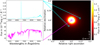Fig. E.1 Simulated scene of the PDS70 system, with the PDS70 star and the PDS70 b and c protoplanets. Top-left: Spectrum of the protoplanets. Bottom-left: Spectrum of the star. They are both degraded by the LSF of the instrument as well as multiplied by a telluric absorption spectrum modeling the effect of the Earth atmosphere. Right: Spectrally integrated image of all the monochromatic images. Stellar and planetary fluxes are spread by the FSF of the instrument resulting in the masking of the planets because of their very low contrast compared to the star. The random noise is negligible compared with the stellar nuisance.

Fig. E.1 sums up the simulated scene, with the planetary and stellar spectra (including LSF spreads), as well as the spectrally integrated image of the three objects (including FSF spreads).

Appendix F ROC curve construction process

Fig. F.1 General ROC curve construction diagram. The first step is the injection of fake planets into real data cubes, at different separations and contrasts. The second step is the recovery of the planetary information from these data cubes using the two stellar halo subtraction methods. The third step is the determination of the probabilities of false alarm and detection following the variation of the planet detection validation threshold. The ROC curve depends directly on these last two variables.

Appendix G Noise statistics

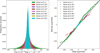Fig. G.1 Normalized histograms and quantile-quantile plots of post-subtraction residual noise (from the 821 spectral channels of the median cube of the post-subtraction residuals of PDS70 images indicated in App. C, with our proposed method following the parameters indicated in Tab. 1). Each monochromatic image is separated into concentric rings (Andres 1994) grouped by 3 to distinguish distributions by separation at the center. Due to stellar residuals and possibly photon noise, the noise standard deviation is greater in the center, as shown in the figure on the left, and its distribution deviates from a Gaussian distribution, as shown in the figure on the right. On the contrary, as the separation increases, the standard deviation decreases and the distribution approaches a Gaussian distribution.

All Tables

All Figures

	Fig. 1 Toy model with rectangular line and flat neighboring continuum. companion emission spectrum. Moreover, being non-linear and non-parametric, it prevents regularization and further extensions. Alternatively, spline-based models for complex halos/speckles thus have also emerged (Agrawal et al. 2023; Ruffio et al. 2023).
In the text

	Fig. 2 Signal processing steps leading to post-subtraction planetary spaxel estimates. (a) Data spaxel ratio with regard to the reference spectrum. (b) Low-pass filtering with Savitzky-Golay filter. (c) Stellar spaxel estimation with overfitting. (d) Planetary spaxel estimation with self-subtraction.
In the text

Fig. 3 Subtraction results at the position of a planet with the SGF method. Left: Overlapping simulation (ground truth) and estimation of the stellar spaxel. There is no emission line in this simulation. Middle: The green spaxel is the estimation of the planetary spaxel, while the cyan one is the associated ground truth. The self-subtraction problem is clearly visible in this situation. Right: The reason for the self-subtraction is evidenced. This is the deformation estimation, in light pink, overfitting the planetary line component of the data to stellar spectrum estimation ratio, in purple. Yet, this overfitting is relatively greater than the planetary and stellar continuum-to-line ratios are different. The real deformation is in dark pink.

In the text

	Fig. 4 Same as Fig. 3, but with a small stellar line (total flux of 5 × 10−13 erg s−1 cm−2 Å−1 in the 6560.3-6565.3 Å band).
In the text

	Fig. 5 Same as Fig. 4, but with a brighter stellar line (total flux of 5 × 10−12 erg s−1 cm−2 Å−1 in the 6560.3-6565.3 Å band).
In the text

	Fig. 6 MSE decomposition at planet position at Hα line wavelength, following Eq. (B.5). The MSE (solid green line) is the sum of the noise overfitting error (dashed yellow line), planets overfitting error (dashdot-ted turquoise line), and star underfitting error (dotted orangy line).
In the text

Fig. 7 Maps of the polynomial coefficients of estimation of the stellar spaxels of real data of observation of the PDS70 system. The color scale is saturated at the 25% and 75% quartiles and centered on 0 by extension in the negative or in the positive (except for the degree of 0 coefficient as corresponding to the total flux). For each spaxel, before estimating the coefficients, each modulation by the base polynomials is L2 normalized (after subtraction of the average, except for the degree of 0, responsible for the total flux). Various spatial components of the PSF are identifiable thanks to the orthogonality of the polynomial basis used. Notably, the degree of 0 and 1 coefficient maps reveal the diffraction spikes in addition to the AO radius, the degree of 2 and 3 coefficient maps reveal other related patterns as well as the heart of the Airy disk, and the degree of 4 and more coefficient maps reveal the secondary rings of the Airy disk (with their outward displacement as the degree of the polynomial increases).

In the text

Fig. 8 Energy share curves of the estimated polynomial coefficients for each of the degrees (except that of degree of 0 as accounting for the total flux and not for the variations) of the basis of decomposition. Before estimating each of the coefficients (except that of degree of 0), the modulations by the base polynomials are, firstly, subtracted from their average, secondly, L2 normalized. For each degree, the energy share is calculated as the median over the field of view of the squared coefficients, divided by the sum of all the median squared coefficients (except that of degree of 0). This was done for PDS70, HTLup, and YSES1 data cubes, each time for individual exposure. This shows that the degree of 4 polynomial coefficients are the last useful ones. Above, the energy of the high-degree coefficients converges towards a minimum where it is mainly fitting noise. It can be seen here that this minimum is reached for the degree of 5 for each of the 23 observations data, indicating that this choice may well generalize.

In the text

	Fig. 9 Spatio-spectral match filtering of the median PDS70 data cube, after stellar halo subtraction by the SGF (left) and LPM (right) methods. A Gaussian is chosen for the spectral model to search for Hα line signal. The corresponding pre-subtraction monochromatic images are chosen for the spatial model to search for spatial PSF patterns.
In the text

	Fig. 10 5-σ contrast curve of both the SGF and LPM methods with 50% detection in solid line as well as 25% and 75% delimiting colored areas. Planets PDS70 b and c are also placed at their contrast and separation. Both are detected by both methods.
In the text

Fig. 11 Bundle of ROC curves, for both halo subtraction methods, and for various fake planet injections separations; a zoom for FAP between 0 and 10−2 is included. The random classifier, which validates or invalidates detections with the same probability of 0.5 is shown as a dotted diagonal line for comparison. AUC stands for area under the curve; by definition, the AUC of the random classifier is equal to 0.5. Contrast curves are located on ROC curves at DP = 0.5 (and 0.25 and 0.75 to built error margins as in Fig. 10 for example) and FAP = 2.87 × 10−7 (corresponding to a 5-σ confidence interval). Data is lacking to produce an accurate curve, especially around FAP = 2.87 × 10−7, but this still shows that, within the 1-σ margin of error, the two stellar halo subtraction methods have relatively equivalent overall robustness as well.

In the text

Fig. 12 HTLup B spectrum estimates by the SGF (in blue) and LPM (in orange) methods. The Hα, Hβ, and [OI] lines as well as the CaII infrared triplet are detected by the SGF method. Absorptions of TiO and Na are revealed by the LPM method in addition, thanks to its greater preservation of the continuum. On the contrary, it reveals the absence of any VO absorptions, suggesting that the star should be a late-M type. Further improvements of the LPM method are planned to improve the continuum recovery and its quantification (see Sect. 4.2) so that it would be indeed usable for physical interpretations. Yet, a more complex study is beyond the scope of this paper, which is primarily focused on the Hα line (or, similarly, any other emission line).

In the text

Fig. 13 YSES1 b spectrum estimates, by the SGF (in blue) and LPM (in orange) methods. Left: zoom in on 821 channels around the Hα line. The self-subtraction caused by the SGF method as well as its correction by the proposed LPM method are visible. Two HeI lines are also revealed. Right: zoom in on 821 channels around the CaII infrared triplet. The self-subtraction around the lines is less visible here, because both the lines are weaker and the continuum is (likely) stronger at these wavelengths (yet, in turn, the heights of the lines are theoretically further underestimated); the mask used by the LPM method during this estimation process was adapted to cover the full triplet. A noticeable Na absorption is also revealed.

In the text

Fig. 14 Zoom in on 51 channels around the Hα (left) and Hβ (right) lines of the YSES1 b spectrum estimates, from stellar halo subtraction, both with the SGF (in blue) and LPM (in orange) methods. The horizontal dots indicate the zero-flux level, i.e., the theoretical flux lower bound. Colored areas delimit the 1-σ confidence intervals with regard to noise. Dotted Gaussians are fitted to the lines to estimate their main parameters (presented in the legend, with confidence intervals derived from Gaussian fits to the lower and upper bounds of those of the spectrum estimates).

In the text

	Fig. A.1 Spatio-spectral simulation of a star observation. On the right, three monochromatic images are shown at wavelengths λ1, λ1841, λ3681 to highlight the spatial spread variation with wavelength. On the left, three spaxels are shown at three different separations to highlight the spectrum deformation caused by this spatial spread variation.
In the text

Fig. A.2 General principle of the SGF stellar halo subtraction method presented in Haffert et al. (2019). Each planetary spaxel (in green) is estimated by subtraction from the data (in black) of an estimate of the stellar spaxel (in red). This latter is estimated by entrywise product of the stellar spectrum estimate (in orange) by the deformation coefficient estimate (in pink). This estimate is made by low-pass filtering of the stellar spectrum estimate to data spaxel ratio (in purple).

In the text

Fig. A.3 General principle of the LPM stellar halo subtraction method we propose. Each planetary spaxel (in green) is estimated by subtraction from the data (in black) of an estimate of the stellar spaxel (in red). This latter is estimated by polynomial modulation (in pink) of the stellar spectrum estimate (in orange). In practice, this is done by multiplication of the data spaxel by the orthogonal projection matrix onto the column space of the design matrix of the polynomial modulation (in brown).

In the text

	Fig. B.1 Simple peak model sampled in wavelengths and deformations.
In the text

Fig. D.1 Fake planet recovery by both stellar halo subtraction methods (SGF on the left and LPM on the right) after injection in YSES1 b observation cubes. The cyan spaxel is the one of the simulated planet injected in the cubes. The green spaxel is the mean of its estimations by stellar halo subtraction along the 9 cubes. The light green area covers this mean more or less the standard deviation computed along the 9 cubes at each wavelength. The fake planets were injected at separations of 0.44” (first line), 0.85” (second line), 1.69” (third line), and 2.10” (fourth line). The horizontal dots delimit the 100%, 50%, 10% and 0% of the height of the simulated line (normalized to 100). The vertical dots delimit the line wavelengths from the continuum wavelengths used for MSE calculations.

In the text

Fig. E.1 Simulated scene of the PDS70 system, with the PDS70 star and the PDS70 b and c protoplanets. Top-left: Spectrum of the protoplanets. Bottom-left: Spectrum of the star. They are both degraded by the LSF of the instrument as well as multiplied by a telluric absorption spectrum modeling the effect of the Earth atmosphere. Right: Spectrally integrated image of all the monochromatic images. Stellar and planetary fluxes are spread by the FSF of the instrument resulting in the masking of the planets because of their very low contrast compared to the star. The random noise is negligible compared with the stellar nuisance.

In the text

Fig. F.1 General ROC curve construction diagram. The first step is the injection of fake planets into real data cubes, at different separations and contrasts. The second step is the recovery of the planetary information from these data cubes using the two stellar halo subtraction methods. The third step is the determination of the probabilities of false alarm and detection following the variation of the planet detection validation threshold. The ROC curve depends directly on these last two variables.

In the text

Fig. G.1 Normalized histograms and quantile-quantile plots of post-subtraction residual noise (from the 821 spectral channels of the median cube of the post-subtraction residuals of PDS70 images indicated in App. C, with our proposed method following the parameters indicated in Tab. 1). Each monochromatic image is separated into concentric rings (Andres 1994) grouped by 3 to distinguish distributions by separation at the center. Due to stellar residuals and possibly photon noise, the noise standard deviation is greater in the center, as shown in the figure on the left, and its distribution deviates from a Gaussian distribution, as shown in the figure on the right. On the contrary, as the separation increases, the standard deviation decreases and the distribution approaches a Gaussian distribution.

In the text

References

- Agrawal, S., Ruffio, J.-B., Konopacky, Q. M., et al. 2023, ApJ, 166, 15 [Google Scholar]
- Alarcón, F., Bergin, E. A., & Cugno, G. 2024, ApJ, 966, 225 [Google Scholar]
- Allard, F., Homeier, D., & Freytag, B. 2011, in Astronomical Society of the Pacific Conference Series, 448, 16th Cambridge Workshop on Cool Stars, Stellar Systems, and the Sun, 91 [Google Scholar]
- Allard, F., Homeier, D., & Freytag, B. 2012, Philos. Trans. Roy. Soc. Lond. Ser. A, 370, 2765 [NASA ADS] [Google Scholar]
- Andres, E. 1994, Comput. Graph., 18, 695 [Google Scholar]
- Aoyama, Y., & Ikoma, M. 2019, ApJ, 885, L29 [NASA ADS] [CrossRef] [Google Scholar]
- Aoyama, Y., Marleau, G.-D., Mordasini, C., & Ikoma, M. 2020, arXiv e-prints [arXiv:2011.06608] [Google Scholar]
- Aoyama, Y., Marleau, G.-D., & Hashimoto, J. 2024, AJ, 168, 155 [Google Scholar]
- Arsenault, R., Madec, P. Y., Hubin, N., et al. 2008, SPIE Conf. Ser., 7015, 701524 [NASA ADS] [Google Scholar]
- Bacon, R., Accardo, M., Adjali, L., et al. 2010, in Ground-based and Airborne Instrumentation for Astronomy III, 7735, International Society for Optics and Photonics (SPIE), 773508 [Google Scholar]
- Barber, M. G., Thao, P. C., Mann, A. W., et al. 2024, ApJ, 973, L30 [Google Scholar]
- Batygin, K. 2018, AJ, 155, 178 [NASA ADS] [CrossRef] [Google Scholar]
- Betti, S. K., Follette, K. B., Ward-Duong, K., et al. 2022, ApJ, 935, L18 [NASA ADS] [CrossRef] [Google Scholar]
- Betti, S. K., Follette, K. B., Ward-Duong, K., et al. 2023, AJ, 166, 262 [Google Scholar]
- Beuzit, J.-L., Vigan, A., Mouillet, D., et al. 2019, A&A, 631, A155 [NASA ADS] [CrossRef] [EDP Sciences] [Google Scholar]
- Biddle, L. I., Bowler, B. P., Zhou, Y., Franson, K., & Zhang, Z. 2024, AJ, 167, 172 [NASA ADS] [CrossRef] [Google Scholar]
- Bohn, A. J., Kenworthy, M. A., Ginski, C., et al. 2020a, MNRAS, 492, 431 [Google Scholar]
- Bohn, A. J., Kenworthy, M. A., Ginski, C., et al. 2020b, ApJ, 898, L16 [Google Scholar]
- Bouma, L. G., Hartman, J. D., Brahm, R., et al. 2020, AJ, 160, 239 [Google Scholar]
- Chaushev, A., Sallum, S., Lozi, J., et al. 2024, AJ, 168, 70 [Google Scholar]
- Chauvin, G., Lagrange, A.-M., Zuckerman, B., et al. 2005, A&A, 438, L29 [NASA ADS] [CrossRef] [EDP Sciences] [Google Scholar]
- Cugno, G., Quanz, S. P., Hunziker, S., et al. 2019, A&A, 622, A156 [NASA ADS] [CrossRef] [EDP Sciences] [Google Scholar]
- Cugno, G., Patapis, P., Stolker, T., et al. 2021, A&A, 653, A12 [NASA ADS] [CrossRef] [EDP Sciences] [Google Scholar]
- Cumming, A., Helled, R., & Venturini, J. 2018, MNRAS, 477, 4817 [Google Scholar]
- Currie, T., Lawson, K., Schneider, G., et al. 2022, Nat. Astron., 6, 751 [NASA ADS] [CrossRef] [Google Scholar]
- De Rosa, R. J., Nielsen, E. L., Wahhaj, Z., et al. 2023, A&A, 672, A94 [NASA ADS] [CrossRef] [EDP Sciences] [Google Scholar]
- Demars, D., Bonnefoy, M., Dougados, C., et al. 2023, A&A, 676, A123 [NASA ADS] [CrossRef] [EDP Sciences] [Google Scholar]
- Eriksson, S. C., Asensio Torres, R., Janson, M., et al. 2020, A&A, 638, L6 [NASA ADS] [CrossRef] [EDP Sciences] [Google Scholar]
- Follette, K. B., Close, L. M., Males, J. R., et al. 2023, AJ, 165, 225 [NASA ADS] [CrossRef] [Google Scholar]
- Guyon, O., Martinache, F., Garrel, V., et al. 2010, SPIE Conf. Ser., 7736, 773624 [Google Scholar]
- Haffert, S., Bohn, A., de Boer, J., et al. 2019, Nat. Astron., 3, 749 [Google Scholar]
- Hashimoto, J., Aoyama, Y., Konishi, M., et al. 2020, AJ, 159, 222 [Google Scholar]
- Heller, R., & Pudritz, R. 2015, ApJ, 806, 181 [NASA ADS] [CrossRef] [Google Scholar]
- Helstrom, C. W. 1994, Elements of Signal Detection and Estimation (USA: Prentice-Hall, Inc.) [Google Scholar]
- Hoch, K., Rowland, M., Petrus, S., et al. 2025, Bull. AAS, 57 [Google Scholar]
- Hoeijmakers, H. J., Schwarz, H., Snellen, I. A. G., et al. 2018, A&A, 617, A144 [NASA ADS] [CrossRef] [EDP Sciences] [Google Scholar]
- Huélamo, N., Chauvin, G., Mendigutía, I., et al. 2022, A&A, 668, A138 [NASA ADS] [CrossRef] [EDP Sciences] [Google Scholar]
- Jorquera, S., Bonnefoy, M., Pérez, L. M., et al. 2024, ApJ, 976, 42 [Google Scholar]
- Julo, R., Chatelain, F., Bonnefoy, M., et al. 2024, in 32nd European Signal Processing Conference (EUSIPCO) [Google Scholar]
- Kay, S. M. 1997, Fundamentals of Statistical Signal Processing: Estimation Theory (Prentice Hall) [Google Scholar]
- Keppler, M., Benisty, M., Müller, A., et al. 2018, A&A, 617, A44 [NASA ADS] [CrossRef] [EDP Sciences] [Google Scholar]
- Lagrange, A.-M., Bonnefoy, M., Chauvin, G., et al. 2010, Science, 329, 57 [Google Scholar]
- Lagrange, A. M., Meunier, N., Rubini, P., et al. 2019, Nat. Astron., 3, 1135 [NASA ADS] [CrossRef] [Google Scholar]
- Macintosh, B., Graham, J. R., Ingraham, P., et al. 2014, PNAS, 111, 12661 [NASA ADS] [CrossRef] [Google Scholar]
- Mann, A. W., Newton, E. R., Rizzuto, A. C., et al. 2016, AJ, 152 [Google Scholar]
- Marleau, G.-D., Aoyama, Y., Kuiper, R., et al. 2022, A&A, 657, A38 [NASA ADS] [CrossRef] [EDP Sciences] [Google Scholar]
- Marley, M. S., Fortney, J. J., Hubickyj, O., Bodenheimer, P., & Lissauer, J. J. 2007, ApJ, 655, 541 [Google Scholar]
- Marois, C., Doyon, R., Racine, R., et al. 2005, JRASC, 99, 130 [NASA ADS] [Google Scholar]
- Marois, C., Macintosh, B., Barman, T., et al. 2008, Science, 322, 1348 [Google Scholar]
- Moehler, S., Modigliani, A., Freudling, W., et al. 2014, A&A, 568, A9 [NASA ADS] [CrossRef] [EDP Sciences] [Google Scholar]
- Mordasini, C., Marleau, G.-D., & Mollière, P. 2017, A&A, 608, A72 [NASA ADS] [CrossRef] [EDP Sciences] [Google Scholar]
- Müller, A., Keppler, M., Henning, T., et al. 2018, A&A, 617, L2 [Google Scholar]
- Petrus, S., Bonnefoy, M., Chauvin, G., et al. 2021, A&A, 648, A59 [EDP Sciences] [Google Scholar]
- Pierens, A., & Raymond, S. 2016, MNRAS, 462, 4130 [NASA ADS] [CrossRef] [Google Scholar]
- Plavchan, P., Barclay, T., Gagné, J., et al. 2020, Nature, 582, 497 [Google Scholar]
- Réfrégier, P., Fade, J., & Roche, M. 2007, Opt. Lett., 32, 739 [Google Scholar]
- Ringqvist, S. C., Viswanath, G., Aoyama, Y., et al. 2023, A&A, 669, L12 [NASA ADS] [CrossRef] [EDP Sciences] [Google Scholar]
- Ruffio, J.-B., Horstman, K., Mawet, D., et al. 2023, ApJ, 165, 113 [Google Scholar]
- Sallum, S., Follette, K., Eisner, J., et al. 2015, Nature, 527, 342 [Google Scholar]
- Seber, G., & Lee, A. 2012, Linear Regression Analysis, Wiley Series in Probability and Statistics (Wiley) [Google Scholar]
- Ströbele, S., La Penna, P., Arsenault, R., et al. 2012, SPIE Conf. Ser., 8447, 844737 [Google Scholar]
- Szulágyi, J., & Ercolano, B. 2020, ApJ, 902, 126 [CrossRef] [Google Scholar]
- Thanathibodee, T., Calvet, N., Bae, J., Muzerolle, J., & Hernández, R. F. 2019, ApJ, 885, 94 [NASA ADS] [CrossRef] [Google Scholar]
- Uyama, T., Tanigawa, T., Hashimoto, J., et al. 2017, AJ, 154, 90 [NASA ADS] [CrossRef] [Google Scholar]
- Uyama, T., Norris, B., Jovanovic, N., et al. 2020, J. Astron. Telesc. Instrum. Syst., 6, 045004 [Google Scholar]
- Uyama, T., Xie, C., Aoyama, Y., et al. 2021, AJ, 162, Art. No. 214 [NASA ADS] [CrossRef] [Google Scholar]
- Wagner, K., Follette, K. B., Close, L. M., et al. 2018, AJ, 863, L8 [Google Scholar]
- Wang, J., Vigan, A., Lacour, S., et al. 2021, AJ, 161, 148 [NASA ADS] [CrossRef] [Google Scholar]
- Weilbacher, P. M., Palsa, R., Streicher, O., et al. 2020, A&A, 641, A28 [NASA ADS] [CrossRef] [EDP Sciences] [Google Scholar]
- Xie, C., Haffert, S. Y., de Boer, J., et al. 2020, A&A, 644, A149 [EDP Sciences] [Google Scholar]
- Zhang, Y., Snellen, I. A., Bohn, A. J., et al. 2021, Nature, 595, 370 [NASA ADS] [CrossRef] [Google Scholar]
- Zhou, Y., Bowler, B. P., Wagner, K. R., et al. 2021, AJ, 161, 244 [NASA ADS] [CrossRef] [Google Scholar]
- Zurlo, A., Cugno, G., Montesinos, M., et al. 2020, A&A, 633, A119 [NASA ADS] [CrossRef] [EDP Sciences] [Google Scholar]
The set of the ℓ first integers is denoted as ![Mathematical equation: $[\ell]=\{1,\ldots,\ell\}$](/articles/aa/full_html/2025/11/aa53231-24/aa53231-24-eq129.png)
The set of the ∂ +1 first integers including 0 is denoted as [[∂]]