| Issue |
A&A
Volume 703, November 2025
|
|
|---|---|---|
| Article Number | A201 | |
| Number of page(s) | 23 | |
| Section | Planets, planetary systems, and small bodies | |
| DOI | https://doi.org/10.1051/0004-6361/202553968 | |
| Published online | 20 November 2025 | |
TOI-283 b: A transiting mini-Neptune in a 17.6-day orbit discovered with TESS and ESPRESSO
1
Instituto de Astrofísica de Canarias (IAC),
E-38205
La Laguna, Tenerife,
Spain
2
Departamento de Astrofísica, Universidad de La Laguna (ULL),
38206
La Laguna, Tenerife,
Spain
3
Observatoire Astronomique de l’Université de Genève,
Chemin Pegasi 51b,
1290
Versoix,
Switzerland
4
Lund Observatory, Division of Astrophysics, Department of Physics, Lund University,
Box 118,
22100
Lund,
Sweden
5
Instituto de Astrofísica de Andalucía (IAA-CSIC), Glorieta de la Astronomía s/n,
18008
Granada,
Spain
6
Instituto de Astrofísica e Ciências do Espaço, Universidade do Porto, CAUP, Rua das Estrelas,
4150-762
Porto,
Portugal
7
Departamento de Física e Astronomia, Faculdade de Ciências, Universidade do Porto, Rua do Campo Alegre,
4169-007
Porto,
Portugal
8
Centro de Astrobiología, CSIC-INTA, Camino Bajo del Castillo s/n,
28692
Villanueva de la Cañada, Madrid,
Spain
9
Physics Institute of University of Bern,
Gesellschafts strasse 6,
3012
Bern,
Switzerland
10
SOAR Telescope/NSF NOIRLab,
Casilla 603,
La Serena,
Chile
11
SETI Institute, Mountain View, CA 94043 USA/NASA Ames Research Center,
Moffett Field,
CA
94035,
USA
12
NASA Exoplanet Science Institute, Caltech/IPAC,
Mail Code 100-22, 1200 E. California Blvd.,
Pasadena,
CA
91125,
USA
13
Center for Astrophysics | Harvard & Smithsonian,
60 Garden Street,
Cambridge,
MA
02138,
USA
14
George Mason University,
4400 University Drive,
Fairfax,
VA
22030,
USA
15
INAF – Osservatorio Astronomico di Trieste,
Via Tiepolo 11,
34143
Trieste,
Italy
16
NASA Ames Research Center,
Moffett Field,
CA
94035,
USA
17
Gemini Observatory/NSF’s NOIRLab,
670 A’ohoku Place,
Hilo,
HI
96720,
USA
18
Department of Physics and Astronomy, The University of North Carolina at Chapel Hill,
Chapel Hill,
NC
27599-3255,
USA
19
Bay Area Environmental Research Institute,
Moffett Field,
CA
94035,
USA
20
European Southern Observatory,
Av. Alonso de Cordova, 3107, Vitacura,
Santiago de Chile,
Chile
21
Centro de Astrofísica da Universidade do Porto, Rua das Estrelas,
4150-762
Porto,
Portugal
22
INAF – Osservatorio Astronomico di Palermo,
Piazza del Parlamento 1,
90134
Palermo,
Italy
23
Instituto de Astrofísica e Ciências do Espaço, Faculdade de Ciências da Universidade de Lisboa, Campo Grande,
1749-016,
Lisboa,
Portugal
24
Consejo Superior de Investigaciones Científicas (CSIC),
28006
Madrid,
Spain
25
Department of Physics and Kavli Institute for Astrophysics and Space Research, Massachusetts Institute of Technology,
Cambridge,
MA
02139,
USA
26
Department of Earth, Atmospheric and Planetary Sciences, Massachusetts Institute of Technology,
Cambridge,
MA
02139,
USA
27
Department of Aeronautics and Astronautics, MIT,
77 Massachusetts Avenue,
Cambridge,
MA
02139,
USA
28
INAF – Osservatorio Astrofisico di Torino, Strada Osservatorio,
20 10025
Pino Torinese (TO),
Italy
29
Department of Astrophysical Sciences, Princeton University,
Princeton,
NJ
08544,
USA
30
Department of Physics, Engineering and Astronomy, Stephen F. Austin State University,
1936 North St,
Nacogdoches,
TX
75962,
USA
★ Corresponding author: This email address is being protected from spambots. You need JavaScript enabled to view it.
Received:
30
January
2025
Accepted:
14
September
2025
Abstract
Context. Super-Earths and mini-Neptunes are missing from our Solar System, yet they appear to be the most abundant planetary types in our Galaxy. A detailed characterization of key planets within this population is important for understanding the formation mechanisms of rocky and gas giant planets and the diversity of planetary interior structures.
Aims. In 2019, NASA’s TESS satellite found a transiting planet candidate in a 17.6-day orbit around the star TOI-283. We started radial velocity (RV) follow-up observations with ESPRESSO to obtain a mass measurement. Mass and radius are measurements critical for planetary classification and internal composition modeling.
Methods. We used ESPRESSO spectra to derive the stellar parameters of the planet candidate host star TOI-283. We then performed a joint analysis of the photometric and RV data of this star, using Gaussian processes to model the systematic noise present in both datasets.
Results. We find that the host is a bright K-type star (d = 82.4 pc, Teff = 5213 ± 70 K, V = 10.4 mag) with a mass and radius of M⋆ = 0.80 ± 0.01 M⊙ and R⋆ = 0.85 ± 0.03 R⊙. The planet has an orbital period of P = 17.617 days, a size of Rp = 2.34 ± 0.09 R⊕, and a mass of Mp = 6.54 ± 2.04 M⊕. With an equilibrium temperature of ~600 K and a bulk density of ρp = 2.81 ± 0.93 g cm−3, this planet is positioned in the mass-radius diagram where planetary models predict H2O- and H/He-rich envelopes. The ESPRESSO RV data also reveal a long-term trend that is probably related to the star’s activity cycle. Further RV observations are required to confirm whether this signal originates from stellar activity or another planetary body in the system.
Key words: techniques: photometric / techniques: radial velocities / planets and satellites: detection / planets and satellites: individual: TOI-283b / stars: individual: TOI-283
© The Authors 2025
 Open Access article, published by EDP Sciences, under the terms of the Creative Commons Attribution License (https://creativecommons.org/licenses/by/4.0), which permits unrestricted use, distribution, and reproduction in any medium, provided the original work is properly cited.
This article is published in open access under the Subscribe to Open model. This email address is being protected from spambots. You need JavaScript enabled to view it. to support open access publication.
1 Introduction
Ongoing observational efforts, such as those from space telescopes like CoRoT (Baglin et al. 2006), Kepler (Borucki et al. 2010), and TESS (Transiting Exoplanet Survey Satellite, Ricker et al. 2015), have led to the discovery of many transiting exoplanets, allowing for comprehensive statistical population analysis. One of the main results of these population studies is the fact that small exoplanets exhibit a bimodal distribution of radii, characterized by two distinct populations with peaks at Rp ~ 1.3 R⊕ (super-Earths) and Rp ~ 2.4 R⊕ (sub-Neptunes), and separated by a gap referred to as the radius valley (Fulton et al. 2017). Various explanations for this phenomenon focus on mechanisms of atmospheric mass loss, such as photoevaporation driven by the host star (Owen & Wu 2017; Jin & Mordasini 2018) or the internal heating of the planet (Ginzburg et al. 2018). Models based on photoevaporation suggest that super-Earth and sub-Neptunian planets share a rocky composition, and their different radii result from whether they retain a primordial hydrogen/helium atmosphere (H/He envelope). In contrast, if these planets had an icy internal composition, the radius valley would manifest at larger planetary radii (Owen & Wu 2017; Rogers & Owen 2021). Another possible explanation for the origin of the radius valley is that both populations form in different regions of the disk, with super-Earths forming in drier environments (within the water-ice line of the disk) and sub-Neptunes forming beyond the water-ice line and having more water-rich compositions (e.g., Venturini et al. 2020; Burn et al. 2024). Some observational evidence suggests that, at least for M-dwarf hosts, the radius valley may be a consequence of internal composition rather than an indicator of atmospheric mass loss (Luque & Pallé 2022).
In terms of radii, sub-Neptunes have sizes ranging from about 1.5 to 4 R⊕. Sub-Neptunian planets are among the most common types of planet in our Galaxy (Borucki et al. 2011; Fulton et al. 2018), and have been a focus of interest because they represent a transition in planetary characteristics (Fulton et al. 2018; Christiansen et al. 2023). The presence and composition of the atmosphere play a crucial role in determining the overall properties of sub-Neptune planets. Some may have thick atmospheres, possibly composed of hydrogen and helium, similar to gas giants. However, their bulk composition may be a mixture of rocks and volatiles such as water, methane, and ammonia (Zeng et al. 2016, 2019). Nevertheless, sub-Neptunes can be found at various distances from their host stars, and their orbital characteristics vary widely. There is a limited sample of sub-Neptunes that have relatively long periods (P > 15 days) and low stellar irradiances (S < 30 S⊕) and are situated around stars bright enough to allow for atmospheric studies with current instrumentation (V < 12 mag). According to the PlanetS catalog1 (Otegi et al. 2020; Parc et al. 2024), there are only 16 planets that fulfill these characteristics; hence, any addition to this population will have an impact on the study of long-period sub-Neptunes.
The TESS mission is conducting a comprehensive survey of the entire sky to detect transiting planets. Since its launch in mid-2018, TESS has released over 7000 candidate planets, known as TESS objects of interest (TOIs)2. The vast majority of these TOIs require ground-based follow-up observations to confirm their planetary nature, in particular radial velocity (RV) measurements to determine planetary masses. Exploiting the synergies between TESS and ESPRESSO (Pepe et al. 2021), an echelle spectrograph mounted on the VLT in Chile has already led to the discovery and characterization of several small transiting planets around different types of stars (Sozzetti et al. 2021; Palle et al. 2021; Lillo-Box et al. 2021; Demangeon et al. 2021; Bourrier et al. 2022; Barros et al. 2022; Lavie et al. 2023; Damasso et al. 2023).
Here we use ESPRESSO observations to determine the mass of a transiting candidate around TOI-283, which was part of the guaranteed time observations (GTO) sample designed to cover the parameter space of small planets in and around the radius valley. The planet candidate was validated using a statistical approach in Giacalone et al. (2021), in which TOI-283 b was found to have a false positive probability (FPP) of FFP = 0.05 and a nearby false positive probability (NFPP) of NFPP = 1.76 × 10⁻³. According to the Giacalone et al. (2021) validation criteria, this puts this candidate on the edge of their “likely planet” category (FFP < 0.5 and NFPP < 10−3). In addition, Lester et al. (2021) obtained high-angular-resolution imaging observations of 517 host stars of TESS exoplanet candidates using the ’Alopeke and Zorro speckle cameras at Gemini North and South. For TOI-283, they found the star to be single and obtained 5σ Δmag contrast limits at 0.2″ and 1.0″ in the blue filter (562 nm) of 4.61 and 4.97 magnitudes, respectively. In the red filter (832 nm) the values were 5.52 and 7.51 magnitudes. These ground-based validations triggered the start of ESPRESSO observations for mass determination.
The paper is organized as follows. In Sections 2 and 3 we describe the space- and ground-based observations used in this study. Section 4 describes our method of obtaining the stellar parameters of TOI-283 from high-resolution spectra. In Section 5 we present our analysis and results. Finally, in Section 6 we present a discussion of the planet, and in Section 7 we present our conclusions.
2 Space-based observations
2.1 TESS photometry
The planet candidate around TOI-283 was discovered by TESS. The star has a TESS Input Catalog (Stassun et al. 2018) number of TIC 382626661. Due to its near polar declination (δ ~ −65°), TESS observes this target almost continuously for nearly 6 months when the satellite is collecting data from the southern hemisphere.
The analysis and processing of TESS data is performed by the TESS Science Processing Operations Center (SPOC, Jenkins et al. 2016) at the NASA Ames Research Center. The TESS simple aperture photometry (SAP, Morris et al. 2020) light curves are analyzed with a reduction process that begins with the removal of systematic effects using the Presearch Data Conditioning (PDC) pipeline module (Smith et al. 2012; Stumpe et al. 2012, 2014), then a search for transit-like signals is performed using a wavelet-based adaptive, noise-compensating matched filter (Jenkins 2002; Jenkins et al. 2010, 2020). Finally a transit model that includes the effect of limb darkening (Li et al. 2019) is fit to the data. To rule out some false positive scenarios, some validation tests are applied to the time series (Twicken et al. 2018), including the difference image centroid test, which constrains the location of the host star to within 1.7 ± 2.7″ of the transit source in the analysis of sectors 1–69. This result constrains any background source to 1/3 of a pixel at 3σ and complements high-resolution imaging, since the difference image centroid test is sensitive to sources within the stamp, which typically subtends 3.85′ on each side (11 × 11 pixels). The TESS Science Office (TSO) at the Massachusetts Institute of Technology (MIT) evaluates the target reports, and if the candidate passes the validation tests, it is assigned a TOI number. The TSO announced the detection of a transiting planet candidate around TIC 382626661 on 7 May 2019, and assigned the TOI number TOI 283.01. The detected transit event has a period of P ~ 17.6 days and a depth of 722 parts per million (ppm).
To study the transit events of the planet candidate orbiting TOI-283, we used the TESS PDCSAP photometry, covering a total of 36 sectors. Table 1 summarizes the 2-minute cadence TESS data analyzed in this work. The TESS observations span a baseline of 2449 days, with the flux standard deviation per sector ranging from 810 to 926 ppm. Figure A.1 presents the TESS light curves for each sector.
We note that the TESS pixel scale is ~21″, and photometric apertures typically extend to about 1′, which generally results in multiple stars blending into the TESS photometric aperture. Therefore, we used the TESS contamination tool TESS-cont3 (Castro-González et al. 2024) to quantify the flux fraction within the SPOC aperture coming from TOI-283 and nearby sources, and to evaluate whether the observed transit signal could have originated from one of the contaminant stars. We constructed the point response functions (PRFs)4 of the 224 nearby Gaia DR2 sources (Gaia Collaboration 2018) around TOI-283 in a radius of 200″, and the total flux contributions across the TPFs were calculated. In Figure A.2, we summarize the TESS-cont output for Sector 1. We find that 99.5% of the flux comes from TOI-283, indicating a very low degree of contamination. As a sanity check, we also ran TESS-cont based on the DR3 catalog (Gaia Collaboration 2023) and reached the same conclusion. The five most contaminating stars are TIC 382627415 (Star 1), TIC 382626679 (Star 2), TIC 382626664 (Star 3), TIC 382626686 (Star 4), and TIC 382627418 (Star 5), all of which (except Star 3) are outside the SPOC aperture (see Figure A.2). We used the TESS-cont DILUTION function to calculate the necessary eclipse depths to generate the observed 722 ppm transit feature, and found eclipses of 71% (Star 1), 102% (Star 2), 123% (Star 3), 126% (Star 4), and 140% (Star 5). Therefore, we conclude that only Star 1 (TIC 382627415) could have produced the observed transit signal, although it would have to present extremely deep (~70%) eclipses.
Figure A.3 presents the periodogram analysis of the SAP photometry, aimed at constraining the stellar rotation period. A more detailed discussion is provided in Sect. 5.2.
TOI-283 TESS observations with 2-minute cadence used in this work.
2.2 Gaia assessment
We used Gaia DR3 (Gaia Collaboration 2023) to identify potential wide companions associated with TOI-283. Typically, these stars are already cataloged in the TESS Input Catalog, and their influence on the derived transit parameters has been taken into account in the TESS light curves. We searched the Gaia DR3 catalog for common proper motion companions of TOI-283 within a radius of 1° and applied a parallax constraint, selecting stars with parallaxes within 10% of that of TOI-283. The query returned only TOI-283, indicating that it does not share motion and distance with any other star within one degree, according to the magnitude depth probed by Gaia.
Gaia’s astrometric data provide additional insights into the possible presence of nearby stellar companions that may have gone undetected by both Gaia and high-resolution imaging techniques. The Gaia renormalized unit weight error (RUWE) acts as an indicator similar to a reduced χ2, with values of around ≲1.4 indicating that the astrometric solution is consistent with that of a single star. On the other hand, RUWE values of ≳1.4 indicate an excess of astrometric noise, which may suggest the existence of an undetected companion (e.g., Ziegler et al. 2020). TOI-283, with a RUWE of 1.1, supports this single-star interpretation, suggesting that there are no hidden companions contributing additional astrometric noise.
3 Ground-based observations
3.1 LCO photometric follow-up
To attempt to determine the true source of the TESS detection, we acquired ground-based time-series follow-up photometry of the field around TOI-283 as part of the TESS Followup Observing Program (TFOP; Collins 2019)5. We used the TESS Transit Finder, which is a customized version of the Tapir software package (Jensen 2013), to schedule our transit observations.
We observed a partial transit window of TOI-283.01 in Sloan r′ band on UTC 26 January 2019 from the Las Cumbres Observatory Global Telescope (LCOGT; Brown et al. 2013) 1 m network node at the Cerro Tololo Inter-American Observatory in Chile (CTIO). The 1 m telescope is equipped with a 4096 × 4096 SINISTRO camera that has an image scale of 0.389″ per pixel, resulting in a 26′ × 26′ field of view and the images were calibrated by the standard LCOGT BANZAI pipeline (McCully et al. 2018), and differential photometric data were extracted using AstroImageJ (Collins et al. 2017). We used circular photometric apertures of 6.2" that excluded all of the flux from the nearest known neighbor in the Gaia DR3 catalog (Gaia DR3 5275527777289351040, Gaia Collaboration 2023) that is 41.4″ east of TOI-283. An on-time ~775 ppm ingress was detected on-target (see Figs. B.1 and B.2). Additionally, we checked for possible nearby eclipsing binaries (NEBs) that could be contaminating the TESS photometric aperture and causing the TESS detection. To account for possible contamination from the wings of neighboring star PSFs, we searched for NEBs out to 2.5′ from TOI-283. If fully blended in the SPOC aperture, a neighboring star that is fainter than the target star by 7.9 magnitudes in TESS-band could produce the SPOC-reported flux deficit at mid-transit (assuming a 100% eclipse). To account for possible TESS magnitude uncertainties and possible delta-magnitude differences between TESS-band and Sloan r′, we included an additional threshold of 0.5 mag for fainter objects (down to TESS-band magnitude 17.5). We calculated the root mean square (RMS) of each of the 32 nearby star light curves (binned in 10-minute bins) that meet our search criteria and find that the values are smaller by at least a factor of 5 compared to the required NEB depth in each respective star. We then visually inspected each neighboring star’s light curve to ensure no obvious eclipse-like signal. Our analysis ruled out an NEB blend as the cause of the SPOC pipeline TOI-283.01 detection in the TESS data. All light curve data are available on the EXOFOP-TESS website6.
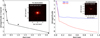 |
Fig. 1 High-resolution images of TOI-283. Left panel: SOAR/HRCam observation of TOI-283 taken on 18 February 2019. No nearby stars were detected within 3″. Inset: thumbnail image of TOI-283. Right panel: Gemini/Zorro high-resolution image of TOI-283 taken on 7 April 2024. TOI-283 is a single star to a contrast limit of 7 mag at 832 nm. Inset: 1.2″ × 1.2″ thumbnail image of TOI-283. |
3.2 High-resolution imaging
As part of our validation process, we observed TOI-283 using high-resolution imaging to place some constraints on the presence of nearby star-bound sources and/or faint background stars not detected by the seeing limited photometric observations. These sources may introduce some unaccounted flux contamination that could affect the TESS photometry, resulting in an underestimated planetary radius, or be the source of astrophysical false positives, such as background eclipsing binaries.
3.2.1 SOAR/HRCam
We searched for stellar companions to TOI-283 with speckle imaging on the 4.1 m Southern Astrophysical Research (SOAR) telescope (Tokovinin 2018) on 18 February 2019, observing in the Cousins I-band, a similar visible bandpass to TESS. This observation was sensitive with 5-sigma detection to a 5.4-magnitude fainter star at an angular distance of 1 arcsec from the target. More details of the observations within the SOAR TESS survey are available in Ziegler et al. (2020). The 5σ detection sensitivity and speckle autocorrelation functions from the observations are shown in Figure 1. No nearby stars were detected within 3″ of TOI-283 in the SOAR observations.
3.2.2 Gemini/Zorro
We observed TOI-283 on two nights (16 March 2020 and 7 April 2023) with the Zorro speckle imager (Scott et al. 2021) on the 8.1 m Gemini South telescope. This instrument contains a dichroic that diverts the input beam from the telescope to two electron-multiplying CCD imagers that operate simultaneously in different bandpasses. For our observations, we used filters centered on 562 nm and 832 nm. For the 2020 observation, 5000 frames, each with an exposure time of 60 milliseconds, were obtained in both filters, while for the 2023 observation, 6000 frames were obtained using the same filters. After observing TOI-283, we observed a nearby point source and reduced the data using techniques described by Howell et al. (2011) and Horch et al. (2011).
Figure 1 presents the results of the observations taken on 7 April 2023. No stellar companions were detected with Zorro between 1.2″ and 0.02″ (the inner limit at 562 nm). The observations have typical 5σ limits of 7 mag at 832 nm and 4.8 mag at a separation between 0.1″ and 1.2″ (equivalent to projected separations of 8–99 AU adopting a distance d = 83 pc), although the detection limits become increasingly shallow inside of 0.1″.
3.3 ESPRESSO high-resolution spectroscopy
We obtained high-resolution spectroscopic observations of TOI-283 with the ESPRESSO spectrograph (Pepe et al. 2014, 2021) installed at the 8.2-m Very Large Telescope (VLT) at Paranal Observatory, Chile. During the observing campaign, we collected a total of 95 measurements, from which we selected a subset to be used in the final fit. Previous works based on ESPRESSO data have shown that instrumental effects can affect the RV measurements. These effects can be traced using telemetry data from the spectrograph (see, for example, Suárez Mascareño et al. 2023, 2024). As selection criteria, we retained only those measurements for which the atmospheric dispersion corrector (ADC) operated without technical issues and the temperature of the instrument’s optical elements remained within 5σ of the median value across the entire dataset. According to these criteria, out of a total of 95 measurements, 11 exhibited ADC-related issues, while none showed temperature-related anomalies. In this work, we analyze a total of 84 high-resolution spectra acquired between 9 February 2019 and 12 February 2022, spanning a time baseline of 1172 days. The data were reduced with the data reduction software (DRS) v.3.0.07. The DRS obtains RV measurements by performing a Gaussian fit to the cross-correlation function (CCF) of the spectrum, which is generated using a binary mask derived from a stellar template (Fellgett 1955; Baranne et al. 1996; Pepe et al. 2000). The RV measurements exhibit a standard deviation of 7.4 m s−1, while the median RV uncertainty is 0.53 m s−1 with a standard deviation of 0.11 m s−1.
The DRS also provides several stellar activity index values calculated from the CCF, including the full width at half-maximum (FWHM) of the CCF, the bisector inverse slope (BIS) derived from the CCF, and the contrast (CONT) of the CCF (Zechmeister & Kürster 2009). In addition to the CCF related values, the DRS also delivers some line activity indices such as the Mount Wilson chromospheric S index computed from the Ca II H & K lines (λλ396.8 nm, 393.3 nm; Vaughan et al. 1978), Na I doublet (λλ589.0 nm, 589.6 nm), and Hα (λ656.2 nm). Table C.1, available at the CDS, presents the RV measurements and activity indices used in this work. Figure D.1 shows the RV measurements versus the activity index values, after subtracting the median from each dataset (E18 and E19) separately, along with the corresponding Pearson correlation coefficient (r). No strong correlation (i.e., |r| > 0.7) was found between the radial velocities and activity measurements.
During the period in which the RVs were collected, the ESPRESSO spectrograph underwent an intervention in June-July 2019 to replace the fiber link, which improved the efficiency of the instrument by 50% (Pepe et al. 2021) and introduced an offset into the measurements. To account for the potential offset caused by the intervention, we considered two datasets in our modeling: the observations before the intervention (E18) and the data after the intervention (E19) (see Section 5.4). Figure 2 shows the observations of the ESPRESSO RV time series.
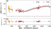 |
Fig. 2 TOI-283 b RV measurements taken with ESPRESSO. Panel a: RV time series and best-fitting model. The best-fitting model was computed using the median values of the posterior distribution of the fit parameters; the shaded area represents the 1σ uncertainty limits of the best-fitting model. Panel b: residuals of the fit after subtracting the single-planet Keplerian model. The uncertainties shown here include the RV jitter values (added in quadrature) for each set. |
4 Stellar properties
The general stellar properties of TOI-283 are presented in Table 2. The stellar atmospheric parameters (Teff, log g, microturbulence, [Fe/H]) were derived using ARES+MOOG, following the same methodology described in Santos et al. (2013); Sousa (2014); Sousa et al. (2021). The ARES code8 (Sousa et al. 2007, 2015) was used to consistently measure the equivalent widths (EWs) of selected iron lines based on the linelist presented in Sousa et al. (2008). This was done on a combined ESPRESSO spectrum of TOI-283. We used a minimization process to find the ionization and excitation equilibrium and converge to the best set of spectroscopic parameters. This process makes use of a grid of Kurucz model atmospheres (Kurucz 1993) and the radiative transfer code MOOG (Sneden 1973). In the end, we found the converged parameters that are listed in Table 2. The trigonometric surface gravity was also derived using Gaia DR3 data following the same methodology as described in Sousa et al. (2021).
The age, mass, and radius were inferred using the Bayesian code PARAM9 (da Silva et al. 2006; Rodrigues et al. 2014, 2017). The code follows a grid-based approach, whereby a well-sampled grid of stellar evolutionary tracks is matched to the observed quantities Teff, [Fe/H], and luminosity. Although the first two inputs were taken from this study, the luminosity was computed by converting the bolometric magnitude. Specifically, it was calculated from the observed magnitudes B and V (Høg et al. 2000), G (Gaia Collaboration 2021), J, H, and Ks (Skrutskie et al. 2006), corrected by the corresponding bolometric correction and for the distance. All bolometric corrections were estimated using the online tool YBC10 (PARSEC Bolometric Correction; Chen et al. 2019) with the input quantities Teff, [Fe/H], and log g). The distance is instead calculated from the inverse of the parallax (Gaia EDR3, Gaia Collaboration 2021). The final luminosity (L = 0.456 ± 0.016 L⊙) was calculated as the weighted average of all the luminosities derived from the photometric bands considered. The grid of stellar evolutionary tracks is from MESA (Paxton et al. 2011, 2013, 2015, 2018, 2019), computed with the physics described in Moedas et al. (2022), grid D1, and with a helium enrichment law of ΔY/ΔZ = 1.23 (from solar calibration) and an extended mass range of M = [0.7 − 1.8] M⊙. The final age, mass, and radius are listed in Table 2.
Using the activity indices described in Sect. 3.3, we measured a median S index of 0.191 ± 0.045; this translates to a log10(R′HK) of −4.92 ± 0.23 using the calibration of Noyes et al. (1984)11. The rotation period of the star was derived from the time series of the activity indices; the methodology is described in Sect. 5.2.
Stellar parameters of TOI-283.
5 Analysis and results
5.1 TESS light curve analysis
To obtain initial estimates of the period and epoch of the transit event, we conducted an independent analysis of 32 of the 36 available TESS sectors. This subset was selected in order to reduce computational costs, as processing the full dataset is resource-intensive. We began by removing long-term stellar or instrumental trends from the PDCSAP light curves using a Python implementation of the Savitzky–Golay filter (Savitzky & Golay 1964). For each TESS sector, the light curve was normalized by dividing it by a smoothed version of itself, computed with a 48-hour time window. To search for transit events, we used the Transit Least Squares algorithm (TLS, Hippke & Heller 2019)12. The dataset analyzed by TLS contained approximately 510 700 data points spanning a baseline of ~1880 days. Within a search range of 0.6 to 940.6 days, TLS detected a periodic transit-like signal with a period of P = 17.61731 ± 0.00184 days and a false alarm probability (FAP) of 8 × 10⁻⁵, consistent with the period reported by TESS.
Figure 3 shows the signal detection efficiency (SDE) as a function of period (top panel) and the phase-folded TESS light curve at the period with the maximum SDE. This result confirms that our reduced-data analysis successfully recovers the known transiting signal. Furthermore, no additional significant periodic signals were found, suggesting the absence of a second transiting planet in the system. These results are in agreement with the more detailed analysis presented in Section 5.6.
5.2 Stellar rotation
We analyzed the ESPRESSO activity indices time series to look for periodic signals that could be caused by the star’s rotation. To model the time series of the FWHM, BIS, CONT, S index, Na, Hα, and Ca indices, we used a combination of a third-degree polynomial to model any long-term trend present in the data and a periodic term using Gaussian processes (GP; e.g., Rasmussen & Williams 2010; Gibson et al. 2012). Each individual curve was modeled independently using a time-dependent function described by
![Mathematical equation: $\[A(t)=a+b t+c t^2+d t^3,\]$](/articles/aa/full_html/2025/11/aa53968-25/aa53968-25-eq3.png) (1)
(1)
where a is the zero point, and b, c, and d are the linear, quadratic, and cubic terms of the third-degree polynomial, respectively. To model the systematic noise present in the data, we employed a GP function incorporating a periodic term, specifically the periodic kernel described in Foreman-Mackey et al. (2017):
![Mathematical equation: $\[k_{i j ~\mathrm{P}}(t)=\frac{B}{2+C} \exp ^{-\left|t_i-t_j\right| / L}\left[\cos \left(\frac{2 \pi\left|t_i-t_j\right|}{P_{\text {rot }}}\right)+(1+C)\right],\]$](/articles/aa/full_html/2025/11/aa53968-25/aa53968-25-eq4.png) (2)
(2)
where |ti − tj| is the difference between two epochs or observations, Prot is the period of the variation, and the constants B, C, and L are all positive and greater than 0. In addition to the parameters that describe the long-term trend and the GP hyperparameters, we included a jitter term to estimate the white noise present in each time series.
We estimated the values of the constants of the third-degree polynomial (a, b, c, and d), the GP kernel (B, C, L, and P), and the jitter terms using a Bayesian Markov chain Monte Carlo (MCMC) procedure. The priors used for fitting each parameter are presented in Table 3. The fitting procedure started with the optimization of a log posterior function using PyDE13. Once the PyDE converged to a solution, we used this solution as a starting point and ran emcee (Foreman-Mackey et al. 2013) for 25 000 iterations using 70 chains (with a thin value of 50). For the fit parameters, we computed the percentiles of the posterior distribution as our final values (median) and 1σ uncertainty range.
Figure 4 shows the distribution of the fit rotation period (Prot) derived from each activity index, while Table 4 summarizes the final rotation period estimates and their associated uncertainties. Of all the activity indicators, only FWHM exhibits a well-defined peak in its posterior distribution, yielding Prot = ![Mathematical equation: $\[30.0_{-4.1}^{+5.8}\]$](/articles/aa/full_html/2025/11/aa53968-25/aa53968-25-eq12.png) days. Other indices, such as BIS and Hα, also show peaks near 30 days, though with larger uncertainties. The remaining activity indicators display broader posterior distributions without significant peaks. The rotation period derived from FWHM is consistent with the expected value of Prot = 28 ± 12 days predicted by the activity-rotation relationship of Suárez Mascareño et al. (2015).
days. Other indices, such as BIS and Hα, also show peaks near 30 days, though with larger uncertainties. The remaining activity indicators display broader posterior distributions without significant peaks. The rotation period derived from FWHM is consistent with the expected value of Prot = 28 ± 12 days predicted by the activity-rotation relationship of Suárez Mascareño et al. (2015).
In addition, we analyzed the TESS SAP photometry and searched for long-term photometric archival data that could confirm the rotation period found by our analysis of stellar activity indices. The generalized Lomb-Scargle (GLS, Lomb 1976; Scargle 1982; Zechmeister & Kürster 2009) periodogram of the TESS SAP data (see Fig. A.3) shows that the most significant power peak is around 33 days. This value is consistent with the rotation period found in our analysis, although they are close to the total baseline of a TESS single-sector observation, which is ~27 days, with the spacecraft sending data to Earth and stopping observations every ~13.5 days. Thus, it is possible that the signals detected in the periodogram of the TESS data could be associated with systematics introduced by the orbit of the satellite.
Searching for archival data, we found two TOI-283 time series taken by the All-Sky Automated Survey for Supernovae (ASAS-SN, Shappee et al. 2014). The ASAS-SN Sky Patrol portal14 provided light curves in the V and g bands with a large number of measurements and baselines greater than ~1600 days, but the data show a large scatter and the GLS periodograms of the light curves do not show a significant peak around ~30 days for both bands.
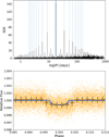 |
Fig. 3 TLS analysis of TESS light curves. Top panel: signal detection efficiency (SDE) versus period. The peak with the maximum SDE corresponds to P = 17.61731 ± 0.00184 days. Bottom panel: TESS light curve folded to the maximum SDE period. The blue line corresponds to the TLS transit model. |
Priors for the parameters used to fit the activity indices.
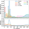 |
Fig. 4 Stellar rotation from activity indices. Top panel: histograms of the posterior distribution of the fit rotation period for the ESPRESSO activity indices. Bottom panel: kernel density estimation of the posterior distributions. |
Derived Prot values from the activity indices.
5.3 Radial velocity and activity indices frequency analysis
To search for the planetary signal in our ESPRESSO data, we computed the GLS periodogram for the RV measurements and activity indices. To generate the GLS periodograms for each variable, we used the Python implementation of Zechmeister & Kürster (2009)15. Figure 5 shows the GLS periodograms, with the orbital period of TOI-283 b marked with a vertical red line. The periodograms were computed using the RV and activity index values after subtracting the median of each dataset, separately for the pre- (E18) and post- (E19) intervention epochs. The FAP levels shown in the figure were calculated using Eq. (24) from Zechmeister & Kürster (2009).
Despite the relatively large number of observations and the long time baseline covered by the ESPRESSO data, the RV periodogram does not show a significant peak at the expected orbital period of the TOI-283 b transit events. As is shown in Fig. 2, the RV data may have a long-term trend that could hinder the detection of the transiting planet candidate in the periodogram. As a test, we fit the RV dataset using different approaches to model the presence of the candidate and the long-term trend. We tested four models: 1) a single Keplerian with no trend, 2) a single Keplerian plus a linear trend, 3) a single Keplerian plus a quadratic trend, and 4) a two Keplerian model. The planet-induced RV variation was modeled as a Keplerian assuming a circular orbit, and we used normal priors for the period and central time of the transiting candidate based on TESS estimates. The fitting procedure was similar to that described in Sect. 5.2, in which we optimized a posterior function and then applied an MCMC procedure to obtain the posterior probability distributions of the fit parameters. Depending on the complexity of the model we had between seven and ten free parameters and ran the MCMC for 15 000 iterations using 80 chains. To evaluate the goodness of fit, we computed the Bayesian information criterion (BIC) metric (Schwarz 1978) for each model using the best-fit parameters. The BIC metric is defined as
![Mathematical equation: $\[\mathrm{BIC}=k ~\ln (n)-2 ~\ln (\hat{L}),\]$](/articles/aa/full_html/2025/11/aa53968-25/aa53968-25-eq13.png) (3)
(3)
where ![Mathematical equation: $\[\hat{L}\]$](/articles/aa/full_html/2025/11/aa53968-25/aa53968-25-eq14.png) is the maximized likelihood, n is the number of data points, and k is the number of fit parameters. In this framework, models with lower BIC values are preferred. In our case, the model with the lowest BIC value was model 4, i.e., the two-planet model.
is the maximized likelihood, n is the number of data points, and k is the number of fit parameters. In this framework, models with lower BIC values are preferred. In our case, the model with the lowest BIC value was model 4, i.e., the two-planet model.
To search for the planetary signal, we fit the long-term variability seen in the RV time series with a second Keplerian function. The second panel from the top in Fig. 5 shows the GLS periodogram of the RV measurements after fitting and removing this long-term trend. The periodogram shows a broad series of discrete peaks around ~8.6 days and ~17.4 days, slightly below the 1% FAP level. While this latter peak periodicity does not match that of the transiting planet, the series of peaks is broad enough to include it.
Similarly, we analyzed the GLS periodograms of several activity indicators derived from the ESPRESSO data. As is shown in Fig. 5, none of these indices exhibit significant periodicities (even at a false positive alarm level of 10%) in the short-period regime (P < 100 days). However, some indicators display peaks around 200–300 days; for example, the FWHM, S index, Hα, and Ca. Additionally, several activity indices (e.g., FWHM, S index, Hα, and Ca) show signs of long-term variability on timescales of ~1000 days; however, these signals are less significant than the peak observed in the RV periodogram.
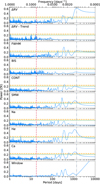 |
Fig. 5 GLS periodograms of the ESPRESSO RVs, activity indices, and the observational window function. The RV and activity index values were median-subtracted for each dataset before (E18) and after (E19) the June–July 2019 intervention. Horizontal lines indicate the FAP levels at 10% (dash-dotted green line) and 1% (dashed orange line). The vertical dotted red line marks the orbital period of TOI-283 b (P = 17.61745 days), while the vertical dash-dotted gray line indicates the period of the long-term signal (P = 1356 days; see Sect. 5.4). |
5.4 Joint fit of TESS and ESPRESSO data
We decided to omit the LCOGT ground-based transit observation from the global fit because the full transit could not be observed and, in addition, the entire event was covered by TESS Sector 7. However, we would like to point out that the LCOGT data provided a transit detection consistent with the TESS results (see Appendix B). We performed a joint fit of the available data (TESS light curves and ESPRESSO RVs) to obtain the candidate orbital and physical properties. We decided to include the entire TESS time series in the fit, with no binning of the observations. We used a Bayesian MCMC approach to fit the data, as is described in Section 5.2 and in Murgas et al. (2023). The transit events were modeled using PyTransit16 (Parviainen 2015). We adopted a quadratic limb darkening (LD) law, during the fit the LD coefficients were compared to the predicted values computed with LDTK17 (Parviainen & Aigrain 2015) using a likelihood function. The predicted LDTK LD values were calculated using the derived stellar parameters presented in Table 2. The ESPRESSO RV measurements were modeled using RadVel18 (Fulton et al. 2018).
Although instrumental effects are removed from the TESS light curves by the PDC algorithm, it is common practice to model the presence of photometric variability and residual systematics with GPs. For the TESS time series, we adopted the commonly used Matérn 3/2 kernel:
![Mathematical equation: $\[k_{i j}=c_k^2\left(1+\frac{\sqrt{3}\left|t_i-t_j\right|}{\tau_k}\right) \exp \left(-\frac{\sqrt{3}\left|t_i-t_j\right|}{\tau_k}\right),\]$](/articles/aa/full_html/2025/11/aa53968-25/aa53968-25-eq15.png) (4)
(4)
where |ti − tj| is the time between epochs in the series, and the hyperparameters, ck and τk, were allowed to be free, with k indicating the different light curves analyzed here.
The use of GPs is also applied to the RV measurements to model any velocity variation induced by the stellar activity of the star. We decided to use the RadVel quasi-periodic (QP) kernel described by
![Mathematical equation: $\[k_{i j ~\mathrm{RV}}=\eta_1^2 \exp \left(\frac{-\left|t_i-t_j\right|^2}{\eta_2^2}-\frac{1}{2 \eta_4^2} \sin ^2\left(\frac{\pi\left|t_i-t_j\right|}{\eta_3}\right)\right),\]$](/articles/aa/full_html/2025/11/aa53968-25/aa53968-25-eq16.png) (5)
(5)
where ti − tj is the time between the epochs in the series, and the hyperparameters, ηi (with i ∈ [1, 4]), were set free. For the period of the kernel (i.e., η3), we used normal priors centered around the stellar rotation period derived from the activity indices (see Sect. 5.2).
To model both time series, we used as free parameters the planet-to-star radius ratio (Rp/R⋆), the LD coefficients (q1, q2 following Kipping 2013), the central time of the transit (Tc), the planetary orbital period (P), the stellar density (ρ⋆), the transit impact parameter (b), and the RV semi-amplitude (K). The longterm trend present in the RVs was modeled using a Keplerian function with its epoch, orbital period, and RV semi-amplitude set as free parameters (see Sect. 5.3). Because we split our RV measurements into two epochs, each subset had its own velocity offset (γ) and RV jitter (σRV jitter). We considered two orbital models: one with a circular orbit (eccentricity fixed at e = 0) and one with an eccentric orbit. For the eccentric model, we used the parameterization ![Mathematical equation: $\[\sqrt{e} ~\cos (\omega)\]$](/articles/aa/full_html/2025/11/aa53968-25/aa53968-25-eq17.png) and
and ![Mathematical equation: $\[\sqrt{e} ~\sin (\omega)\]$](/articles/aa/full_html/2025/11/aa53968-25/aa53968-25-eq18.png) , where ω is the argument of the periastron. Considering the orbital parameters and the GP coefficients for each TESS sector and the RV time series, we had a total of 91 and 93 free parameters for the circular and eccentric models, respectively.
, where ω is the argument of the periastron. Considering the orbital parameters and the GP coefficients for each TESS sector and the RV time series, we had a total of 91 and 93 free parameters for the circular and eccentric models, respectively.
We adopted uniform priors for all parameters except the stellar density, for which we used a normal prior based on the mass and radius values derived from our stellar parameters. Since the transit was detected by TSO and confirmed by our independent analysis presented in Sect. 5.1, we applied more restrictive uniform priors for Tc and P, spanning a range of ±0.4 days around the predicted values. For the TESS GPs, we set a uniform prior in logarithmic space for the timescale hyperparameter (τk), ranging from one hour to half the length of a TESS sector, i.e., 13 days.
The fitting procedure is the same as the one described in Sect. 5.2. We optimized a posterior probability function using the differential evolution routine PyDE. The results of the global optimization procedure were used as a starting point of an MCMC procedure using emcee. We ran emcee using 360 chains for 15 000 iterations as a burn-in phase, and the main MCMC phase was run for 50 000 iterations, while keeping the parameter values of every 100th iteration to reduce autocorrelation. The final values of the fit parameters were computed using the median and 1σ limits of the posterior distributions of the parameters. The prior ranges and the final parameter values with their respective uncertainties are presented in Table 5. The results for the GP hyperparameters are presented in Table E.1.
To determine whether the circular or eccentric model provided a better fit to our data, we compared the difference between the BIC values for the circular and eccentric models. We find a difference of ΔBIC = BICEcc − BICCirc = 28, which means that the circular model is a better fit to our data. It is also worth noting that our eccentric model also finds an orbit solution with a low eccentricity value of e = ![Mathematical equation: $\[0.11_{-0.07}^{+0.11}\]$](/articles/aa/full_html/2025/11/aa53968-25/aa53968-25-eq19.png) , which could be considered consistent with a circular orbit according to the criterion of Lucy & Sweeney (1971). Given the results of the BIC comparison, we adopted the results of the circular orbit fit as our final values for the remainder of the paper.
, which could be considered consistent with a circular orbit according to the criterion of Lucy & Sweeney (1971). Given the results of the BIC comparison, we adopted the results of the circular orbit fit as our final values for the remainder of the paper.
Figure 2 shows the RV time series including the results for the best-fit circular orbit model, Figure 6 shows the final light curve fit to the TESS data and the radial velocities phase-folded to the planet’s orbital period. The RV residuals RMSs are 6.5 m s−1 for the pre-intervention data (E18) and 3.1 m s−1 for the post-intervention measurements (E19); these values were calculated including the fit RV jitter value (added in quadrature) for each set. The relatively large scatter of the residuals could be explained by stellar activity, although no strong correlations between the RVs and the activity indices were found (see Fig. D.1). Figure E.1 shows the posterior distributions for the fit transit and orbital parameters of TOI-283 b.
Figure 7 presents the phase-folded fit to the long-term RV trend. Our Keplerian model fit finds a period of P = ![Mathematical equation: $\[1356_{-179}^{+498}\]$](/articles/aa/full_html/2025/11/aa53968-25/aa53968-25-eq20.png) days and a RV semi-amplitude of K =
days and a RV semi-amplitude of K = ![Mathematical equation: $\[9.4_{-1.6}^{+2.3}\]$](/articles/aa/full_html/2025/11/aa53968-25/aa53968-25-eq21.png) m s−1. If the signal originated from an additional companion in the system, its minimum mass would be Mp sin i =
m s−1. If the signal originated from an additional companion in the system, its minimum mass would be Mp sin i = ![Mathematical equation: $\[0.44_{-0.08}^{+0.12}\]$](/articles/aa/full_html/2025/11/aa53968-25/aa53968-25-eq22.png) MJup, placing it within the planetary regime. However, a compelling alternative explanation is that the long-term trend arises from stellar activity. The GLS periodogram of the activity indicators shown in Fig. 5 reveals significant power at periods around 300–400 days in the FWHM, S index, Hα, and Ca indices. In particular, many of these indices also show peaks above the 1% FAP threshold near the period derived for the long-term RV signal. This alignment strengthens the interpretation that stellar activity may be responsible for the observed trend. Moreover, our RV time span of ~1170 days only marginally covers a single orbit of the proposed companion, complicating any robust planetary interpretation. Additional long-term RV monitoring will be essential to determine whether the trend detected in the ESPRESSO data is indeed caused by a planetary companion or is instead stellar in origin.
MJup, placing it within the planetary regime. However, a compelling alternative explanation is that the long-term trend arises from stellar activity. The GLS periodogram of the activity indicators shown in Fig. 5 reveals significant power at periods around 300–400 days in the FWHM, S index, Hα, and Ca indices. In particular, many of these indices also show peaks above the 1% FAP threshold near the period derived for the long-term RV signal. This alignment strengthens the interpretation that stellar activity may be responsible for the observed trend. Moreover, our RV time span of ~1170 days only marginally covers a single orbit of the proposed companion, complicating any robust planetary interpretation. Additional long-term RV monitoring will be essential to determine whether the trend detected in the ESPRESSO data is indeed caused by a planetary companion or is instead stellar in origin.
In addition to the results presented above, we explored alternative joint fitting strategies by varying the GP treatment of the RV data. These tests were conducted to determine whether it was possible to reduce the level of RV jitter. Specifically, we tested: (i) a fit without including GPs; (ii) a fit with a non-periodic GP kernel (squared exponential); and (iii) a fit including a third Keplerian signal with orbital periods ranging from 0.5 to 15 days and the same QP kernel that was described previously. Across all these tests, the RV jitter values remain consistent, likely because the GP parameters, particularly those describing the exponential timescales, are only weakly constrained. Crucially, the inferred orbital parameters of the transiting planet are unchanged within uncertainties in all cases, demonstrating that the planet’s properties are robustly estimated despite the relatively high levels of RV jitter.
5.5 Transit timing variations
We checked the presence of measurable transit timing variations (TTVs) using TESS photometric data. We utilized PyTTV to fit the transits, treating each central transit time as a free parameter following the method described in Korth et al. (2023). Our search for TTVs involved jointly fitting the TESS photometry of all sectors with PyTTV. The results showed no significant deviations in the transit centers from the linear ephemeris. The TTVs are illustrated in Figure 8.
5.6 Planet searches and detection limits from TESS photometry
We analyzed the TESS 120 s cadence data in the search for hints of potential planetary candidates that remained unnoticed by the SPOC and Quick-Look Pipeline (QLP) pipelines. To this end, we used the SHERLOCK package (Pozuelos et al. 2020; Demory et al. 2020) by combining all available sectors exploring the orbital periods from 1 to 30 d, using ten detrended scenarios corresponding to window sizes ranging from 0.2 to 1.2 d. We refer the reader to Pozuelos et al. (2023) and Dévora-Pajares et al. (2024) for further details about different search strategies.
In the first run, we found a strong signal corresponding to TOI-283 b, which allowed us to independently confirm the detectability of this candidate. In the subsequent runs, SHERLOCK found other weaker signals, all attributable to noise or spurious detections, and hence we did not find any other signal hinting at extra transiting planets in the orbital periods explored.
We then conducted injection and retrieval experiments to establish detection limits. In this context, we used the MATRIX package (Dévora-Pajares & Pozuelos 2022), which produces a set of synthetic planets by integrating various orbital periods, planetary radii, and orbital phases that were inserted into the dataset (see, e.g., Delrez et al. 2022). Due to the vast number of sectors available, this experiment was computationally costly, generating an extremely dense grid of scenarios. Instead, our strategy explored some illustrative combinations of radii, periods, and phases, following Van Grootel et al. (2021). In particular, we used planetary sizes of 1,2, and 3 R⊕, with the orbital periods of 1, 5, 10, 15, 20, 25, and 30 d. Then, each pair of radius-period was evaluated in five different orbital phases. Hence, in total, we explored 105 scenarios. We found that Earth-size planets are 100% recovered when residing in short orbital periods (<10 d), allowing us to rule out the presence of any transiting planet in close-in orbits. However, for orbital periods equal to or larger than 15 d, the recovery of these small planets rapidly decreases to 0%, making them invisible in the data. In contrast, larger planets (2 and 3 R⊕) were easily recovered for the full set of periods explored, with recovery rates larger than 85%, allowing us to conclude that they are likely not present in the system.
Prior functions, and fit and derived parameters of TOI-283 b.
6 Discussion
From our analysis, we determined that TOI-283 b has a radius of Rp = 2.34 ± 0.09 R⊕, a mass of Mp = 6.54 ± 2.04 M⊕, and an orbital period of 17.61 days. The planet orbits its star with a separation of a = 0.123 ± 0.004 au. Assuming a Bond albedo of 0, this leads to an equilibrium temperature of Teq = 661 ± 9 K, while we derive a stellar insolation of Sp = 30.4 ± 2.5 S⊕. Figure 9 places TOI-283 b in a mass-radius diagram of known transiting planets found in the TEPCat19 catalog (Southworth 2011). For illustration purposes, we also include the composition models from Zeng et al. (2016, 2019) with the closest temperature to TOI-283 b (700 K). TOI-283 b occupies a densely populated area of the diagram, where several bulk compositions are plausible, including the presence of significant H/He-rich atmospheres and water-rich planets.
Fulton et al. (2017) and Fulton & Petigura (2018) show that the radii of small planets in short-period orbits (P < 100 days) have a bimodal distribution, with a gap at Rp ~ 1.8 R⊕ separating smaller super-Earths (Rp ~ 1.3 R⊕) from larger sub-Neptunes (Rp ~ 2.4 R⊕). With a planetary radius of Rp = 2.34 ± 0.09 R⊕, this planet is closer to the sub-Neptune population than to the accepted super-Earth regime. Figure 10 shows the period-radius diagram for known transiting planets around K-type stars (4000 K < Teff < 5300 K). We only show planets with radii smaller than 4 R⊕. From the figure is clear that TOI-283 b is above the gap measured by Van Eylen et al. (2018) and the gap position derived by Venturini et al. (2024). Our derived planetary radius is consistent with the majority of the population of sub-Neptunes around K stars.
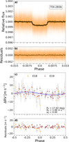 |
Fig. 6 TESS and ESPRESSO phase-folded data of TOI-283 b. Panel a: TOI-283 b phase-folded TESS light curve after subtracting the photometric variations from the time series. The best-fit transit model is shown in black. The circles are TESS binned observations. Panel b: residuals of the transit fit. Panel c: ESPRESSO phase-folded RV measurements and best fit (blue line) after subtracting the quadratic trend and red-noise component. Panel d: residuals of the RV fit. |
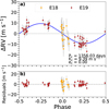 |
Fig. 7 ESPRESSO phase-folded RV time series of the long-term RV trend of TOI-283 (panel a) and the residuals of the fit (panel b). |
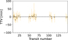 |
Fig. 8 TOI-283 b TTVs from TESS. No significant TTVs are detected in a time baseline of ~2449 days. |
6.1 Planet composition
To better constrain the properties of TOI-283 b, we compared it to the synthetic exoplanet population presented by Venturini et al. (2024)20. In their work, Venturini et al. (2024) model planet formation around stars with masses of 0.1, 0.4, 0.7, 1.0, 1.3, and 1.5 M⊙ using a pebble-accretion formation framework (see also Venturini et al. 2020). Their simulations assume the formation of a single planetary embryo per disk and include planetary migration processes. Following the dispersal of the protoplanetary disk, the models track the planets’ thermal evolution, including cooling and photoevaporation, up to an age of 2 Gyr. Most of the resulting synthetic planets have orbital periods of ~11–18 days. In the left panel of Fig. 11, we present the mass-radius diagram for synthetic planets formed around a 0.7 M⊙ star. TOI-283 b is located in a region populated by planets with water mass fractions exceeding 0.3, suggesting that TOI-283 b may be predominantly water-rich. However, this interpretation must be treated with caution, as the synthetic population models are limited to 2 Gyr. As our stellar age estimates suggest that the TOI-283 system is much older, evolutionary processes such as prolonged atmospheric loss may have significantly altered the planet’s composition beyond the time span considered in these simulations.
In the right panel of Fig. 11, we present a mass-density diagram with the density normalized by the Earth-like composition model from Zeng et al. (2016, 2019). The simulations are able to reproduce the distinct density populations found in M dwarfs by Luque & Pallé (2022). In this case there is a noticeable lack of planets with normalized densities between ρ/ρ⊕,S ~ 0.6–0.8 in agreement with the limit proposed by Luque & Pallé (2022) of ρ/ρ⊕,S ~ 0.65. As with the mass-radius diagram, TOI-283 b’s position places it in the water-rich composition and away from the rocky planet normalized density region. This could indicate that TOI-283 b is a mini-Neptune with a significant amount of water, but Venturini et al. (2024) point out that for planets with Teq > 400 K, as is the case for TOI-283 b with Teq ≈ 660 K, the water layer is in the form of water vapor and not a liquid ocean. This has the effect of increasing the radius of the planet compared to the radii of condensed water worlds.
We used ExoMDN21 (Baumeister & Tosi 2023) to investigate the interior structure of TOI-283 b. ExoMDN is an inference model for planetary interiors based on a mixture density network (MDN) trained on 5.6 million synthetic planet models computed with the TATOOINE code (Baumeister et al. 2020; MacKenzie et al. 2023). The TATOOINE interior models assume compositions consisting of an iron core, a silicate mantle, a water and high-pressure ice layer, and an H/He atmosphere. The training set planets have masses below 25 M⊕ and equilibrium temperatures in the range of 100–1000 K. To produce the ExoMDN interior models, we used as input parameters the mass, radius, and equilibrium temperature of TOI-283 b. In Figure 12 we show the ExoMDN predicted thickness and mass fraction of the interior layers of TOI-283 b. The models predict that the planet consists of an interior structure comprising a ![Mathematical equation: $\[31_{-17}^{+14}\]$](/articles/aa/full_html/2025/11/aa53968-25/aa53968-25-eq51.png) % core, a
% core, a ![Mathematical equation: $\[22_{-20}^{+28}\]$](/articles/aa/full_html/2025/11/aa53968-25/aa53968-25-eq52.png) % mantle, a
% mantle, a ![Mathematical equation: $\[31_{-23}^{+23}\]$](/articles/aa/full_html/2025/11/aa53968-25/aa53968-25-eq53.png) % water layer, and a
% water layer, and a ![Mathematical equation: $\[12_{-10}^{+20}\]$](/articles/aa/full_html/2025/11/aa53968-25/aa53968-25-eq54.png) % gas envelope, where all percentages refer to the respective thicknesses relative to the planetary radius. In terms of mass fraction, TOI-283 b could be dominated by a water envelope with
% gas envelope, where all percentages refer to the respective thicknesses relative to the planetary radius. In terms of mass fraction, TOI-283 b could be dominated by a water envelope with ![Mathematical equation: $\[40_{-32}^{+35}\]$](/articles/aa/full_html/2025/11/aa53968-25/aa53968-25-eq55.png) % of its mass budget occupied by this molecule. This implies that TOI-283 b could be a water-rich planet, in agreement with the composition models shown in Figure 9 and the synthetic population planets of Venturini et al. (2024).
% of its mass budget occupied by this molecule. This implies that TOI-283 b could be a water-rich planet, in agreement with the composition models shown in Figure 9 and the synthetic population planets of Venturini et al. (2024).
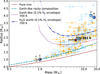 |
Fig. 9 Mass-radius diagram for TOI-283 b (red star) and known transiting planets with mass determinations with a precision better than 30% (parameters taken from the TEPCat database; Southworth 2011). Planets orbiting K-type stars (4000 ≤ Teff ≤ 5300 K) are marked with orange circles. The lines in the mass-radius diagram represent the composition models of Zeng et al. (2016, 2019) for planets with pure iron cores (100% Fe, brown line), Earth-like rocky compositions (32.5% Fe plus 67.5% MgSiO3, dashed green line), Earth-like compositions with a 0.1% H2 envelope (dotted purple line), and a water world with a 0.1% H2 gas envelope (dash-dotted blue line). We show some Solar System planets for reference (Venus, Earth, Uranus, and Neptune). |
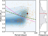 |
Fig. 10 Period-radius diagram for small planets (Rp < 4 R⊕) around K-type stars (4000 K < Teff < 5300 K). The shaded blue area represents a Gaussian kernel density estimation of the points. The position of TOI-283 b is marked by the red star. The dashed olive line shows the position of the radius gap from Van Eylen et al. (2018), while the dotted pink line shows the position of the gap from Venturini et al. (2024). The data were taken from the NASA Exoplanet Archive (https://exoplanetarchive.ipac.caltech.edu/). |
6.2 Atmospheric characterization
To evaluate the potential for atmospheric characterization of TOI-283 b, we calculated the transmission spectroscopy metric (TSM; Kempton et al. 2018), which is proportional to the expected signal-to-noise ratio based on the strength of spectral features. We retrieved a TSM value of 35, which is below the recommended threshold value of 90 for prioritizing planets in the parameter space of TOI-283 b. For completeness the emission spectroscopy metric (ESM) is 1.8, very low, as is expected for a small warm planet. In Figure 13, we plot the TSM value against the J magnitude of the host star, from all known small (Rp < 4 R⊕) planets with radius measurements, including TOI-283 b. This means that transmission spectroscopy with JWST is possible but challenging.
Although JWST observations can be challenging, if this space-based telescope were able to probe the atmosphere of TOI-283 b through transmission spectroscopy, the resulting molecular detections could offer valuable insights into its interior structure and water content. Planets with radii between 1 and 2.6 R⊕, masses between 1 and 10 M⊕, and H2-rich atmospheres containing significant amounts of water in the form of oceans – the so-called Hycean planets (Madhusudhan et al. 2021) – may exhibit distinctive atmospheric signatures. Several studies suggest that Hycean atmospheres can show enhancements in CO2, H2O, and/or CH4, depletion of NH3 due to dissolution in a liquid-water ocean, and enhanced CH3OH abundances (e.g., Hu et al. 2021; Tsai et al. 2021; Madhusudhan et al. 2023; Holmberg & Madhusudhan 2024). The detection (or non-detection) of these species could help differentiate between a water-rich world and one with an Earth-like composition. An additional caveat for TOI-283 b is its high equilibrium temperature (Teq ~ 660 K), which suggests that any water present is likely to be predominantly in the gas phase rather than in liquid form (see previous section). Therefore, predictions developed for Hycean planets near the habitable zone may not be fully applicable to TOI-283 b.
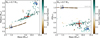 |
Fig. 11 Comparison of TOI-283 b to synthetic planets with short orbital periods (P < 100 days) and an age of 2 Gyr around a 0.7 M⊙ star from the simulations of Venturini et al. (2024). The position of TOI-283 b is marked by the orange star. The planets are marked by dots with the color indicating the fraction of water. Left panel: mass–radius diagram. Right panel: mass–density diagram (density normalized by an Earth-like composition). |
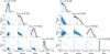 |
Fig. 12 ExoMDN interior modeling results. Left: predicted thickness of the interior layers of TOI-283 b. Right: predicted mass fraction of the interior layers of TOI-283 b. |
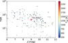 |
Fig. 13 Transmission spectroscopy metric (TSM) versus J band apparent magnitude of known transiting planets with radii of Rp < 4 R⊕. |
7 Conclusions
We report the discovery of TOI-283 b, a sub-Neptunian planet orbiting a K star with an orbital period of 17.6 days. The planet candidate was first detected by NASA’s TESS mission; ground-based observations confirmed that the star has no detectable stellar companions and that the transits occur on the star TOI-283. High-precision RV measurements made with the VLT’s ESPRESSO instrument enabled the mass of the planet candidate to be determined.
We have obtained the stellar parameters of the planet’s host star by analyzing a combined high-resolution ESPRESSO stellar spectrum. Our analysis indicates that TOI-283 has an effective temperature of Teff = 5213 ± 70 K, an iron abundance of [Fe/H] = −0.09 ± 0.05 dex, and a derived stellar mass and radius of M⋆ = 0.80 ± 0.01 M⊙ and R⋆ = 0.85 ± 0.03 R⊙, respectively. From the stellar activity indicators derived from the spectroscopic observations, we estimate a stellar rotation period of about 30 days, with the FWHM indicator having the smallest uncertainty at Prot = ![Mathematical equation: $\[30.0_{-4.1}^{+5.8}\]$](/articles/aa/full_html/2025/11/aa53968-25/aa53968-25-eq56.png) days.
days.
To determine the main orbital parameters of the planet, we jointly fit the light curves of TESS (36 sectors) and 84 RV measurements taken with the ESPRESSO spectrograph. The TESS and ESPRESSO datasets were fit simultaneously using an MCMC procedure, with both time series taking into account the contribution of red noise sources modeled by Gaussian processes. From our best-fit model, we measured an orbital period of P = 17.61745 ± 0.00002 days and derived a planetary radius of Rp = 2.34 ± 0.09 R⊕ and a mass of Mp = 6.54 ± 2.04 M⊕. These values allow us to classify TOI-283 b as a mini-Neptune. The position in the mass-radius diagram of this planet and theoretical compositional models indicate that this planet has a significant contribution from light elements and is consistent with an extended H/He-rich atmosphere and/or significant water content. Given the possibility that TOI-283 b is a water-rich planet, atmospheric characterization with JWST could offer valuable insights into the presence of water in its atmosphere.
The data and model selection criteria indicate the presence of a long-term trend in the RV time series. During the fitting procedure, we modeled this signal with a second Keplerian component. For this long-term trend, we derived a period of P = ![Mathematical equation: $\[1356_{-179}^{+498}\]$](/articles/aa/full_html/2025/11/aa53968-25/aa53968-25-eq57.png) days and a RV semi-amplitude of K =
days and a RV semi-amplitude of K = ![Mathematical equation: $\[9.4_{-1.6}^{+2.3}\]$](/articles/aa/full_html/2025/11/aa53968-25/aa53968-25-eq58.png) m s−1. The GLS periodograms of the stellar activity indices show that several indicators exhibit peaks above the 1% FAP threshold at periods compatible with that of the long-term RV signal, suggesting that the trend could be driven by a stellar activity cycle. Conversely, if the signal originated from an additional companion in the system, the object would have a minimum mass of Mp sin i =
m s−1. The GLS periodograms of the stellar activity indices show that several indicators exhibit peaks above the 1% FAP threshold at periods compatible with that of the long-term RV signal, suggesting that the trend could be driven by a stellar activity cycle. Conversely, if the signal originated from an additional companion in the system, the object would have a minimum mass of Mp sin i = ![Mathematical equation: $\[0.44_{-0.08}^{+0.12}\]$](/articles/aa/full_html/2025/11/aa53968-25/aa53968-25-eq59.png) MJup, placing it within the planetary regime. Further RV observations are required to determine whether this signal is of planetary origin or induced by stellar variability.
MJup, placing it within the planetary regime. Further RV observations are required to determine whether this signal is of planetary origin or induced by stellar variability.
Data availability
Table C.1 is available at the CDS via https://cdsarc.cds.unistra.fr/viz-bin/cat/J/A+A/703/A201.
Acknowledgements
Based on observations collected at the European Organisation for Astronomical Research in the Southern Hemisphere under ESO programme 1102.C-0744. This paper includes data collected by the TESS mission, which are publicly available from the Mikulski Archive for Space Telescopes (MAST). Funding for the TESS mission is provided by NASA’s Science Mission Directorate. Resources supporting this work were provided by the NASA High-End Computing (HEC) Program through the NASA Advanced Supercomputing (NAS) Division at Ames Research Center for the production of the SPOC data products. We acknowledge the use of public TESS data from pipelines at the TESS Science Office and at the TESS Science Processing Operations Center. This research has made use of the Exoplanet Follow-up Observation Program website, which is operated by the California Institute of Technology, under contract with the National Aeronautics and Space Administration under the Exoplanet Exploration Program. This research has made use of the Exoplanet Follow-up Observation Program (ExoFOP; DOI: 10.26134/ExoFOP5) website, which is operated by the California Institute of Technology, under contract with the National Aeronautics and Space Administration under the Exoplanet Exploration Program. This work makes use of observations from the LCOGT network. Part of the LCOGT telescope time was granted by NOIRLab through the Mid-Scale Innovations Program (MSIP). MSIP is funded by NSF. Based in part on observations obtained at the Southern Astrophysical Research (SOAR) telescope, which is a joint project of the Ministério da Ciência, Tecnologia e Inovações (MCTI/LNA) do Brasil, the US National Science Foundation’s NOIRLab, the University of North Carolina at Chapel Hill (UNC), and Michigan State University (MSU). Some of the observations in the paper made use of the High-Resolution Imaging instrument Zorro. Zorro was funded by the NASA Exoplanet Exploration Program and built at the NASA Ames Research Center by Steve B. Howell, Nic Scott, Elliott P. Horch, and Emmett Quigley. Data were reduced using a software pipeline originally written by Elliott Horch and Mark Everett. Zorro was mounted on the Gemini South telescope of the international Gemini Observatory, a program of NSF NOIRLab, which is managed by the Association of Universities for Research in Astronomy (AURA) under a cooperative agreement with the U.S. National Science Foundation on behalf of the Gemini partnership: the U.S. National Science Foundation (United States), National Research Council (Canada), Agencia Nacional de Investigación y Desarrollo (Chile), Ministerio de Ciencia, Tecnología e Innovación (Argentina), Ministério da Ciência, Tecnologia, Inovações e Comunicações (Brazil), and Korea Astronomy and Space Science Institute (Republic of Korea). This work has made use of data from the European Space Agency (ESA) mission Gaia (https://www.cosmos.esa.int/gaia), processed by the Gaia Data Processing and Analysis Consortium (DPAC, https://www.cosmos.esa.int/web/gaia/dpac/consortium). Funding for the DPAC has been provided by national institutions, in particular the institutions participating in the Gaia Multilateral Agreement. We thank the Swiss National Science Foundation (SNSF) and the Geneva University for their continuous support to our planet low-mass companion search programmes. This work has been carried out within the framework of the National Centre of Competence in Research PlanetS supported by the Swiss National Science Foundation. The authors acknowledge support from the Swiss NCCR PlanetS and the Swiss National Science Foundation. This work has been carried out within the framework of the NCCR PlanetS supported by the Swiss National Science Foundation under grants 51NF40182901 and 51NF40205606. F.M. acknowledges financial support from the Agencia Estatal de Investigación del Ministerio de Ciencia, Innovación y Universidades (MCIU/AEI) through grant PID2023-152906NA-I00. J.K. acknowledges support from the Swedish Research Council (Project Grant 2022-04043) and of the Swiss National Science Foundation under grant number TMSGI2_211697. F.J.P. acknowledges financial support from the Severo Ochoa grant CEX2021-001131-S funded by MCIN/AEI/10.13039/501100011033 and Ministerio de Ciencia e Innovación through the project PID2022-137241NB-C43. A.C.-G. is funded by the Spanish Ministry of Science through MCIN/AEI/10.13039/501100011033 grant PID2019-107061GB-C61. K.A.C. and C.N.W. acknowledge support from the TESS mission via subaward s3449 from MIT. The INAF authors acknowledge financial support of the Italian Ministry of Education, University, and Research with PRIN 201278X4FL and the “Progetti Premiali” funding scheme. X.D. acknowledges the support from the European Research Council (ERC) under the European Union’s Horizon 2020 research and innovation programme (grant agreement SCORE No 851555) and from the Swiss National Science Foundation under the grant SPECTRE (No 200021_215200). This work of CJM was financed by Portuguese funds through FCT (Fundação para a Ciência e a Tecnologia) in the framework of the project 2022.04048.PTDC (Phi in the Sky, DOI 10.54499/2022.04048.PTDC). CJM also acknowledges FCT and POCH/FSE (EC) support through Investigador FCT Contract 2021.01214.CEECIND/CP1658/CT0001 (DOI 10.54499/2021.01214.CEECIND/CP1658/CT0001). Co-funded by the European Union (ERC, FIERCE, 101052347). Views and opinions expressed are however those of the author(s) only and do not necessarily reflect those of the European Union or the European Research Council. Neither the European Union nor the granting authority can be held responsible for them. This work was supported by FCT – Fundação para a Ciência e a Tecnologia through national funds and by FEDER through COMPETE2020 – Programa Operacional Competitividade e Internacionalização by these grants: UIDB/04434/2020; UIDP/04434/2020. J.I.G.H., A.S.M., C.A.P., and R.R. acknowledge financial support from the Spanish Ministry of Science, Innovation and Universities (MICIU) projects PID2020-117493GB-I00 and PID2023-149982NB-I00.
References
- Baglin, A., Auvergne, M., Boisnard, L., et al. 2006, in 36th COSPAR Scientific Assembly, 36, 3749 [Google Scholar]
- Bailer-Jones, C. A. L., Rybizki, J., Fouesneau, M., Demleitner, M., & Andrae, R. 2021, AJ, 161, 147 [Google Scholar]
- Baranne, A., Queloz, D., Mayor, M., et al. 1996, A&AS, 119, 373 [NASA ADS] [CrossRef] [EDP Sciences] [Google Scholar]
- Barros, S. C. C., Demangeon, O. D. S., Alibert, Y., et al. 2022, A&A, 665, A154 [NASA ADS] [CrossRef] [EDP Sciences] [Google Scholar]
- Baumeister, P., & Tosi, N. 2023, A&A, 676, A106 [NASA ADS] [CrossRef] [EDP Sciences] [Google Scholar]
- Baumeister, P., Padovan, S., Tosi, N., et al. 2020, ApJ, 889, 42 [Google Scholar]
- Borucki, W. J., Koch, D., Basri, G., et al. 2010, Science, 327, 977 [Google Scholar]
- Borucki, W. J., Koch, D. G., Basri, G., et al. 2011, ApJ, 736, 19 [Google Scholar]
- Bourrier, V., Zapatero Osorio, M. R., Allart, R., et al. 2022, A&A, 663, A160 [NASA ADS] [CrossRef] [EDP Sciences] [Google Scholar]
- Brown, T. M., Baliber, N., Bianco, F. B., et al. 2013, PASP, 125, 1031 [Google Scholar]
- Burn, R., Mordasini, C., Mishra, L., et al. 2024, Nat. Astron., 8, 463 [Google Scholar]
- Castro-González, A., Lillo-Box, J., Armstrong, D. J., et al. 2024, A&A, 691, A233 [NASA ADS] [CrossRef] [EDP Sciences] [Google Scholar]
- Chen, Y., Girardi, L., Fu, X., et al. 2019, A&A, 632, A105 [EDP Sciences] [Google Scholar]
- Christiansen, J. L., Zink, J. K., Hardegree-Ullman, K. K., et al. 2023, AJ, 166, 248 [NASA ADS] [CrossRef] [Google Scholar]
- Collins, K. 2019, in American Astronomical Society Meeting Abstracts, 233, 140.05 [NASA ADS] [Google Scholar]
- Collins, K. A., Kielkopf, J. F., Stassun, K. G., & Hessman, F. V. 2017, AJ, 153, 77 [Google Scholar]
- Cutri, R. M., Wright, E. L., Conrow, T., et al. 2021, VizieR Online Data Catalog: II/328 [Google Scholar]
- da Silva, L., Girardi, L., Pasquini, L., et al. 2006, A&A, 458, 609 [NASA ADS] [CrossRef] [EDP Sciences] [Google Scholar]
- Damasso, M., Rodrigues, J., Castro-González, A., et al. 2023, A&A, 679, A33 [NASA ADS] [CrossRef] [EDP Sciences] [Google Scholar]
- Delrez, L., Murray, C. A., Pozuelos, F. J., et al. 2022, A&A, 667, A59 [NASA ADS] [CrossRef] [EDP Sciences] [Google Scholar]
- Demangeon, O. D. S., Zapatero Osorio, M. R., Alibert, Y., et al. 2021, A&A, 653, A41 [NASA ADS] [CrossRef] [EDP Sciences] [Google Scholar]
- Demory, B. O., Pozuelos, F. J., Gómez Maqueo Chew, Y., et al. 2020, A&A, 642, A49 [NASA ADS] [CrossRef] [EDP Sciences] [Google Scholar]
- Dévora-Pajares, M., & Pozuelos, F. J. 2022, MATRIX: Multi-phAse Transits Recovery from Injected eXoplanets [Google Scholar]
- Dévora-Pajares, M., Pozuelos, F. J., Thuillier, A., et al. 2024, MNRAS, 532, 4752 [CrossRef] [Google Scholar]
- Fellgett, P. 1955, Optica Acta, 2, 9 [NASA ADS] [CrossRef] [Google Scholar]
- Foreman-Mackey, D., Hogg, D. W., Lang, D., & Goodman, J. 2013, PASP, 125, 306 [Google Scholar]
- Foreman-Mackey, D., Agol, E., Ambikasaran, S., & Angus, R. 2017, AJ, 154, 220 [Google Scholar]
- Fulton, B. J., & Petigura, E. A. 2018, AJ, 156, 264 [Google Scholar]
- Fulton, B. J., Petigura, E. A., Howard, A. W., et al. 2017, AJ, 154, 109 [Google Scholar]
- Fulton, B. J., Petigura, E. A., Blunt, S., & Sinukoff, E. 2018, PASP, 130, 044504 [Google Scholar]
- Gaia Collaboration (Brown, A. G. A., et al.) 2018, A&A, 616, A1 [NASA ADS] [CrossRef] [EDP Sciences] [Google Scholar]
- Gaia Collaboration (Brown, A. G. A., et al.) 2021, A&A, 649, A1 [NASA ADS] [CrossRef] [EDP Sciences] [Google Scholar]
- Gaia Collaboration (Vallenari, A., et al.) 2023, A&A, 674, A1 [NASA ADS] [CrossRef] [EDP Sciences] [Google Scholar]
- Giacalone, S., Dressing, C. D., Jensen, E. L. N., et al. 2021, AJ, 161, 24 [Google Scholar]
- Gibson, N. P., Aigrain, S., Roberts, S., et al. 2012, MNRAS, 419, 2683 [NASA ADS] [CrossRef] [Google Scholar]
- Ginzburg, S., Schlichting, H. E., & Sari, R. 2018, MNRAS, 476, 759 [Google Scholar]
- Hippke, M., & Heller, R. 2019, A&A, 623, A39 [NASA ADS] [CrossRef] [EDP Sciences] [Google Scholar]
- Høg, E., Fabricius, C., Makarov, V. V., et al. 2000, A&A, 355, L27 [Google Scholar]
- Holmberg, M., & Madhusudhan, N. 2024, A&A, 683, L2 [NASA ADS] [CrossRef] [EDP Sciences] [Google Scholar]
- Horch, E. P., Gomez, S. C., Sherry, W. H., et al. 2011, AJ, 141, 45 [Google Scholar]
- Howell, S. B., Everett, M. E., Sherry, W., Horch, E., & Ciardi, D. R. 2011, AJ, 142, 19 [Google Scholar]
- Hu, R., Damiano, M., Scheucher, M., et al. 2021, ApJ, 921, L8 [NASA ADS] [CrossRef] [Google Scholar]
- Jenkins, J. M. 2002, ApJ, 575, 493 [Google Scholar]
- Jenkins, J. M., Chandrasekaran, H., McCauliff, S. D., et al. 2010, SPIE Conf. Ser., 7740, 77400D [Google Scholar]
- Jenkins, J. M., Twicken, J. D., McCauliff, S., et al. 2016, SPIE Conf. Ser.,. 9913, 99133E [Google Scholar]
- Jenkins, J. M., Tenenbaum, P., Seader, S., et al. 2020, Kepler Data Processing Handbook: Transiting Planet Search, Kepler Science Document KSCI-19081-003 [Google Scholar]
- Jensen, E. 2013, Tapir: A web interface for transit/eclipse observability, Astrophysics Source Code Library [record ascl:1306.007] [Google Scholar]
- Jin, S., & Mordasini, C. 2018, ApJ, 853, 163 [Google Scholar]
- Kempton, E. M. R., Bean, J. L., Louie, D. R., et al. 2018, PASP, 130, 114401 [Google Scholar]
- Kipping, D. M. 2013, MNRAS, 435, 2152 [Google Scholar]
- Korth, J., Gandolfi, D., Šubjak, J., et al. 2023, A&A, 675, A115 [NASA ADS] [CrossRef] [EDP Sciences] [Google Scholar]
- Kurucz, R. L. 1993, SYNTHE spectrum synthesis programs and line data [Google Scholar]
- Lavie, B., Bouchy, F., Lovis, C., et al. 2023, A&A, 673, A69 [NASA ADS] [CrossRef] [EDP Sciences] [Google Scholar]
- Lester, K. V., Matson, R. A., Howell, S. B., et al. 2021, AJ, 162, 75 [NASA ADS] [CrossRef] [Google Scholar]
- Li, J., Tenenbaum, P., Twicken, J. D., et al. 2019, PASP, 131, 024506 [NASA ADS] [CrossRef] [Google Scholar]
- Lillo-Box, J., Faria, J. P., Suárez Mascareño, A., et al. 2021, A&A, 654, A60 [NASA ADS] [CrossRef] [EDP Sciences] [Google Scholar]
- Lomb, N. R. 1976, Ap&SS, 39, 447 [Google Scholar]
- Lucy, L. B., & Sweeney, M. A. 1971, AJ, 76, 544 [NASA ADS] [CrossRef] [Google Scholar]
- Luque, R., & Pallé, E. 2022, Science, 377, 1211 [NASA ADS] [CrossRef] [Google Scholar]
- MacKenzie, J., Grenfell, J. L., Baumeister, P., et al. 2023, A&A, 671, A65 [NASA ADS] [CrossRef] [EDP Sciences] [Google Scholar]
- Madhusudhan, N., Piette, A. A. A., & Constantinou, S. 2021, ApJ, 918, 1 [NASA ADS] [CrossRef] [Google Scholar]
- Madhusudhan, N., Sarkar, S., Constantinou, S., et al. 2023, ApJ, 956, L13 [NASA ADS] [CrossRef] [Google Scholar]
- McCully, C., Volgenau, N. H., Harbeck, D.-R., et al. 2018, SPIE Conf. Ser., 10707, 107070K [Google Scholar]
- Moedas, N., Deal, M., Bossini, D., & Campilho, B. 2022, A&A, 666, A43 [NASA ADS] [CrossRef] [EDP Sciences] [Google Scholar]
- Morris, R. L., Twicken, J. D., Smith, J. C., et al. 2020, Kepler Data Processing Handbook: Photometric Analysis, Kepler Science Document KSCI-19081-003 [Google Scholar]
- Murgas, F., Castro-González, A., Pallé, E., et al. 2023, A&A, 677, A182 [NASA ADS] [CrossRef] [EDP Sciences] [Google Scholar]
- Noyes, R. W., Hartmann, L. W., Baliunas, S. L., Duncan, D. K., & Vaughan, A. H. 1984, ApJ, 279, 763 [Google Scholar]
- Otegi, J. F., Bouchy, F., & Helled, R. 2020, A&A, 634, A43 [NASA ADS] [CrossRef] [EDP Sciences] [Google Scholar]
- Owen, J. E., & Wu, Y. 2017, ApJ, 847, 29 [Google Scholar]
- Palle, E., Luque, R., Zapatero Osorio, M. R., et al. 2021, A&A, 650, A55 [EDP Sciences] [Google Scholar]
- Parc, L., Bouchy, F., Venturini, J., Dorn, C., & Helled, R. 2024, A&A, 688, A59 [NASA ADS] [CrossRef] [EDP Sciences] [Google Scholar]
- Parviainen, H. 2015, MNRAS, 450, 3233 [Google Scholar]
- Parviainen, H., & Aigrain, S. 2015, MNRAS, 453, 3821 [Google Scholar]
- Paxton, B., Bildsten, L., Dotter, A., & et al. 2011, ApJS, 192, 3 [Google Scholar]
- Paxton, B., Cantiello, M., Arras, P., et al. 2013, ApJS, 208, 4 [Google Scholar]
- Paxton, B., Marchant, P., Schwab, J., et al. 2015, ApJS, 220, 15 [Google Scholar]
- Paxton, B., Schwab, J., Bauer, E. B., et al. 2018, ApJS, 234, 34 [NASA ADS] [CrossRef] [Google Scholar]
- Paxton, B., Smolec, R., Schwab, J., et al. 2019, ApJS, 243, 10 [Google Scholar]
- Pepe, F., Mayor, M., Delabre, B., et al. 2000, SPIE Conf. Ser., 4008, 582 [NASA ADS] [Google Scholar]
- Pepe, F., Molaro, P., Cristiani, S., et al. 2014, Astron. Nachr., 335, 8 [Google Scholar]
- Pepe, F., Cristiani, S., Rebolo, R., et al. 2021, A&A, 645, A96 [NASA ADS] [CrossRef] [EDP Sciences] [Google Scholar]
- Pozuelos, F. J., Suárez, J. C., de Elía, G. C., et al. 2020, A&A, 641, A23 [NASA ADS] [CrossRef] [EDP Sciences] [Google Scholar]
- Pozuelos, F. J., Timmermans, M., Rackham, B. V., et al. 2023, A&A, 672, A70 [NASA ADS] [CrossRef] [EDP Sciences] [Google Scholar]
- Rasmussen, C., & Williams, C. 2010, The MIT Press, 122, 935 [Google Scholar]
- Ricker, G. R., Winn, J. N., Vanderspek, R., et al. 2015, J. Astron. Telesc. Instrum. Syst., 1, 014003 [Google Scholar]
- Rodrigues, T. S., Girardi, L., Miglio, A., et al. 2014, MNRAS, 445, 2758 [Google Scholar]
- Rodrigues, T. S., Bossini, D., Miglio, A., et al. 2017, MNRAS, 467, 1433 [NASA ADS] [Google Scholar]
- Rogers, J. G., & Owen, J. E. 2021, MNRAS, 503, 1526 [NASA ADS] [CrossRef] [Google Scholar]
- Santos, N. C., Sousa, S. G., Mortier, A., et al. 2013, A&A, 556, A150 [NASA ADS] [CrossRef] [EDP Sciences] [Google Scholar]
- Savitzky, A., & Golay, M. J. E. 1964, Analyt. Chem., 36, 1627 [NASA ADS] [CrossRef] [Google Scholar]
- Scargle, J. D. 1982, ApJ, 263, 835 [Google Scholar]
- Schwarz, G. 1978, Ann. Statist., 6, 461 [Google Scholar]
- Scott, N. J., Howell, S. B., Gnilka, C. L., et al. 2021, Front. Astron. Space Sci., 8, 138 [NASA ADS] [CrossRef] [Google Scholar]
- Shappee, B. J., Prieto, J. L., Grupe, D., et al. 2014, ApJ, 788, 48 [Google Scholar]
- Skrutskie, M. F., Cutri, R. M., Stiening, R., et al. 2006, AJ, 131, 1163 [NASA ADS] [CrossRef] [Google Scholar]
- Smith, J. C., Stumpe, M. C., Van Cleve, J. E., et al. 2012, PASP, 124, 1000 [Google Scholar]
- Sneden, C. A. 1973, PhD thesis, The University of Texas at Austin [Google Scholar]
- Sousa, S. G. 2014 arXiv e-prints [arXiv:1407.5817] [Google Scholar]
- Sousa, S. G., Santos, N. C., Israelian, G., Mayor, M., & Monteiro, M. J. P. F. G. 2007, A&A, 469, 783 [NASA ADS] [CrossRef] [EDP Sciences] [Google Scholar]
- Sousa, S. G., Santos, N. C., Mayor, M., et al. 2008, A&A, 487, 373 [NASA ADS] [CrossRef] [EDP Sciences] [Google Scholar]
- Sousa, S. G., Santos, N. C., Adibekyan, V., Delgado-Mena, E., & Israelian, G. 2015, A&A, 577, A67 [NASA ADS] [CrossRef] [EDP Sciences] [Google Scholar]
- Sousa, S. G., Adibekyan, V., Delgado-Mena, E., et al. 2021, A&A, 656, A53 [NASA ADS] [CrossRef] [EDP Sciences] [Google Scholar]
- Southworth, J. 2011, MNRAS, 417, 2166 [Google Scholar]
- Sozzetti, A., Damasso, M., Bonomo, A. S., et al. 2021, A&A, 648, A75 [NASA ADS] [CrossRef] [EDP Sciences] [Google Scholar]
- Stassun, K. G., Oelkers, R. J., Pepper, J., et al. 2018, AJ, 156, 102 [Google Scholar]
- Stumpe, M. C., Smith, J. C., Van Cleve, J. E., et al. 2012, PASP, 124, 985 [Google Scholar]
- Stumpe, M. C., Smith, J. C., Catanzarite, J. H., et al. 2014, PASP, 126, 100 [Google Scholar]
- Suárez Mascareño, A., Rebolo, R., González Hernández, J. I., & Esposito, M. 2015, MNRAS, 452, 2745 [Google Scholar]
- Suárez Mascareño, A., González-Álvarez, E., Zapatero Osorio, M. R., et al. 2023, A&A, 670, A5 [NASA ADS] [CrossRef] [EDP Sciences] [Google Scholar]
- Suárez Mascareño, A., Passegger, V. M., González Hernández, J. I., et al. 2024, A&A, 685, A56 [NASA ADS] [CrossRef] [EDP Sciences] [Google Scholar]
- Tokovinin, A. 2018, PASP, 130, 035002 [Google Scholar]
- Tsai, S.-M., Innes, H., Lichtenberg, T., et al. 2021, ApJ, 922, L27 [NASA ADS] [CrossRef] [Google Scholar]
- Twicken, J. D., Catanzarite, J. H., Clarke, B. D., et al. 2018, PASP, 130, 064502 [Google Scholar]
- Van Eylen, V., Agentoft, C., Lundkvist, M. S., et al. 2018, MNRAS, 479, 4786 [Google Scholar]
- Van Grootel, V., Pozuelos, F. J., Thuillier, A., et al. 2021, A&A, 650, A205 [NASA ADS] [CrossRef] [EDP Sciences] [Google Scholar]
- Vaughan, A. H., Preston, G. W., & Wilson, O. C. 1978, PASP, 90, 267 [Google Scholar]
- Venturini, J., Guilera, O. M., Haldemann, J., Ronco, M. P., & Mordasini, C. 2020, A&A, 643, L1 [NASA ADS] [CrossRef] [EDP Sciences] [Google Scholar]
- Venturini, J., Ronco, M. P., Guilera, O. M., et al. 2024, A&A, 686, L9 [NASA ADS] [CrossRef] [EDP Sciences] [Google Scholar]
- Zacharias, N., Finch, C. T., Girard, T. M., et al. 2013, AJ, 145, 44 [Google Scholar]
- Zechmeister, M., & Kürster, M. 2009, A&A, 496, 577 [CrossRef] [EDP Sciences] [Google Scholar]
- Zeng, L., Sasselov, D. D., & Jacobsen, S. B. 2016, ApJ, 819, 127 [Google Scholar]
- Zeng, L., Jacobsen, S. B., Sasselov, D. D., et al. 2019, PNAS, 116, 9723 [Google Scholar]
- Ziegler, C., Tokovinin, A., Briceño, C., et al. 2020, AJ, 159, 19 [Google Scholar]
Available at: https://dace.unige.ch
Available at https://github.com/castro-gzlz/TESS-cont
The PRFs of each Sector, Camera, and CCD were accessed at https://archive.stsci.edu/missions/tess/models/prf_fitsfiles/start_s0004/
The latest version, ARES v2, can be downloaded from https://github.com/sousasag/ARES
Appendix A TESS data
Figure A.1 shows the TESS time series and the best fit model from our joint fit analysis (see Sect. 5.4). Figure A.3 shows the GLS periodogram of the TESS SAP photometry. Figure A.2 presents the results of the contamination analysis using TESS.
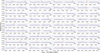 |
Fig. A.1 TOI-283 b TESS light curves analyzed in this work. The black line shows our best model fit. The vertical red lines represent the individual transit events of TOI 283b. |
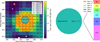 |
Fig. A.2 Nearby sources contributing to the TESS photometry TOI-283. Left: TPF-shaped heatmap with the pixel-by-pixel flux fraction from TOI-283 in S1. The red grid is the SPOC aperture. The white disks represent all the Gaia sources, and the five sources that most contribute to the aperture flux are highlighted in different colours. Disk areas scale with the emitted fluxes. Right: Flux contributions to the SPOC aperture. ‘Other’ refers to the total contamination from nearby Gaia DR2 sources that contribute less than Star 5. |
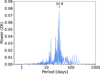 |
Fig. A.3 GLS periodogram of the TESS SAP photometry for the 36 sectors analyzed in this paper. The highest power peak is at a period of ~33 days. |
Appendix B LCOGT transit
Here we describe our fitting process for the LCOGT transit light curve taken on 26 January 2019. For the fit we used a detrended light curve provided by EXOFOP, where the time series was detrended using the FWHM as a proxy for seeing changes during the observations. Similar to our joint fit analysis (see Sect. 5.4), we set as free parameters the planet-to-star radius ratio (Rp/R⋆), the LD coefficients (q1, q2), the central time of the transit (Tc), the planetary orbital period (P), the stellar density (ρ⋆), the transit impact parameter (b), a photometric jitter term to model the white noise component (σphot), and the two GP coefficients of the Matérn 3/2 kernel. Because we had a partial transit, we decided to fit the data using normal priors on Tc, P, and ρ⋆. These priors were derived from the results of a transit fit using only TESS data. After optimizing a posterior probability function with PyDE, we used emcee to sample the posterior with 50 chains and ran an MCMC for 25 000 iterations. The best-fit parameter values and uncertainties were computed from the percentiles of the posterior distributions. Figure B.1 shows the data and the best-fitting model, with our approach we find a planet-to-star radius ratio of Rp/R⋆ = 0.025 ± 0.003 in agreement with TESS measurements (see Fig. B.2). Since this transit event was covered by TESS observations from Sector 7, we decided to omit this dataset from the joint fit.
Appendix C Radial velocity data
In Table C.1 we present the ESPRESSO RV measurements and activity indicators. Table C.1 is only available in electronic form at the CDS via anonymous ftp to cdsarc.u-strasbg.fr (130.79.128.5) or via https://cdsweb.u-strasbg.fr/cgi-bin/qcat?J/A+A/.
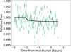 |
Fig. B.1 LCOGT transit observation taken on January 26, 2019. The data were collected with the 1 m telescope at CTIO using a Sloan r′ filter. The black line shows the best-fit model. |
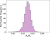 |
Fig. B.2 Posterior distribution of the planet-to-star radius ratio (Rp/R⋆) for the LCOGT transit observation. |
Appendix D Radial velocities and activity indicators
Figure D.1 shows the RV measurements versus the activity indices, after subtracting the median from each dataset (E18 and E19) separately, along with the Pearson product-moment correlation coefficient r between these quantities.
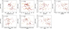 |
Fig. D.1 ESPRESSO RV measurements versus activity indices. In each panel, the Pearson product-moment correlation coefficient r is shown. The RVs and activity indices were median-subtracted separately for the pre- (E18) and post- (E19) intervention datasets. E18 data are shown as orange circles, and E19 data as red squares. |
Appendix E Joint fit of TESS and ESPRESSO data – results
Table E.1 shows the prior ranges and values of the GP hyperparameters for the circular and eccentric orbit fits. Figure E.1 shows the posterior parameter distributions of the joint fit, with the GP parameters for the transit and RV fits intentionally omitted for clarity.
The GP parameters, priors, and fit values for the joint fit.
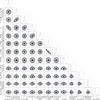 |
Fig. E.1 Corner plot of the posterior distributions of the fit transit and orbital parameters of TOI-283 b. The parameters used to model the systematic effects using GPs have been intentionally left out for ease of viewing. The blue lines mark the median of the distribution. For plotting purposes, the distributions for the central time of the transit and the orbital period have been shifted by Toff = 2459549.0 days and Poff = 17.6174 days, respectively. |
All Tables
All Figures
|
Fig. 1 High-resolution images of TOI-283. Left panel: SOAR/HRCam observation of TOI-283 taken on 18 February 2019. No nearby stars were detected within 3″. Inset: thumbnail image of TOI-283. Right panel: Gemini/Zorro high-resolution image of TOI-283 taken on 7 April 2024. TOI-283 is a single star to a contrast limit of 7 mag at 832 nm. Inset: 1.2″ × 1.2″ thumbnail image of TOI-283. |
| In the text | |
|
Fig. 2 TOI-283 b RV measurements taken with ESPRESSO. Panel a: RV time series and best-fitting model. The best-fitting model was computed using the median values of the posterior distribution of the fit parameters; the shaded area represents the 1σ uncertainty limits of the best-fitting model. Panel b: residuals of the fit after subtracting the single-planet Keplerian model. The uncertainties shown here include the RV jitter values (added in quadrature) for each set. |
| In the text | |
|
Fig. 3 TLS analysis of TESS light curves. Top panel: signal detection efficiency (SDE) versus period. The peak with the maximum SDE corresponds to P = 17.61731 ± 0.00184 days. Bottom panel: TESS light curve folded to the maximum SDE period. The blue line corresponds to the TLS transit model. |
| In the text | |
|
Fig. 4 Stellar rotation from activity indices. Top panel: histograms of the posterior distribution of the fit rotation period for the ESPRESSO activity indices. Bottom panel: kernel density estimation of the posterior distributions. |
| In the text | |
|
Fig. 5 GLS periodograms of the ESPRESSO RVs, activity indices, and the observational window function. The RV and activity index values were median-subtracted for each dataset before (E18) and after (E19) the June–July 2019 intervention. Horizontal lines indicate the FAP levels at 10% (dash-dotted green line) and 1% (dashed orange line). The vertical dotted red line marks the orbital period of TOI-283 b (P = 17.61745 days), while the vertical dash-dotted gray line indicates the period of the long-term signal (P = 1356 days; see Sect. 5.4). |
| In the text | |
|
Fig. 6 TESS and ESPRESSO phase-folded data of TOI-283 b. Panel a: TOI-283 b phase-folded TESS light curve after subtracting the photometric variations from the time series. The best-fit transit model is shown in black. The circles are TESS binned observations. Panel b: residuals of the transit fit. Panel c: ESPRESSO phase-folded RV measurements and best fit (blue line) after subtracting the quadratic trend and red-noise component. Panel d: residuals of the RV fit. |
| In the text | |
|
Fig. 7 ESPRESSO phase-folded RV time series of the long-term RV trend of TOI-283 (panel a) and the residuals of the fit (panel b). |
| In the text | |
|
Fig. 8 TOI-283 b TTVs from TESS. No significant TTVs are detected in a time baseline of ~2449 days. |
| In the text | |
|
Fig. 9 Mass-radius diagram for TOI-283 b (red star) and known transiting planets with mass determinations with a precision better than 30% (parameters taken from the TEPCat database; Southworth 2011). Planets orbiting K-type stars (4000 ≤ Teff ≤ 5300 K) are marked with orange circles. The lines in the mass-radius diagram represent the composition models of Zeng et al. (2016, 2019) for planets with pure iron cores (100% Fe, brown line), Earth-like rocky compositions (32.5% Fe plus 67.5% MgSiO3, dashed green line), Earth-like compositions with a 0.1% H2 envelope (dotted purple line), and a water world with a 0.1% H2 gas envelope (dash-dotted blue line). We show some Solar System planets for reference (Venus, Earth, Uranus, and Neptune). |
| In the text | |
|
Fig. 10 Period-radius diagram for small planets (Rp < 4 R⊕) around K-type stars (4000 K < Teff < 5300 K). The shaded blue area represents a Gaussian kernel density estimation of the points. The position of TOI-283 b is marked by the red star. The dashed olive line shows the position of the radius gap from Van Eylen et al. (2018), while the dotted pink line shows the position of the gap from Venturini et al. (2024). The data were taken from the NASA Exoplanet Archive (https://exoplanetarchive.ipac.caltech.edu/). |
| In the text | |
|
Fig. 11 Comparison of TOI-283 b to synthetic planets with short orbital periods (P < 100 days) and an age of 2 Gyr around a 0.7 M⊙ star from the simulations of Venturini et al. (2024). The position of TOI-283 b is marked by the orange star. The planets are marked by dots with the color indicating the fraction of water. Left panel: mass–radius diagram. Right panel: mass–density diagram (density normalized by an Earth-like composition). |
| In the text | |
|
Fig. 12 ExoMDN interior modeling results. Left: predicted thickness of the interior layers of TOI-283 b. Right: predicted mass fraction of the interior layers of TOI-283 b. |
| In the text | |
|
Fig. 13 Transmission spectroscopy metric (TSM) versus J band apparent magnitude of known transiting planets with radii of Rp < 4 R⊕. |
| In the text | |
|
Fig. A.1 TOI-283 b TESS light curves analyzed in this work. The black line shows our best model fit. The vertical red lines represent the individual transit events of TOI 283b. |
| In the text | |
|
Fig. A.2 Nearby sources contributing to the TESS photometry TOI-283. Left: TPF-shaped heatmap with the pixel-by-pixel flux fraction from TOI-283 in S1. The red grid is the SPOC aperture. The white disks represent all the Gaia sources, and the five sources that most contribute to the aperture flux are highlighted in different colours. Disk areas scale with the emitted fluxes. Right: Flux contributions to the SPOC aperture. ‘Other’ refers to the total contamination from nearby Gaia DR2 sources that contribute less than Star 5. |
| In the text | |
|
Fig. A.3 GLS periodogram of the TESS SAP photometry for the 36 sectors analyzed in this paper. The highest power peak is at a period of ~33 days. |
| In the text | |
|
Fig. B.1 LCOGT transit observation taken on January 26, 2019. The data were collected with the 1 m telescope at CTIO using a Sloan r′ filter. The black line shows the best-fit model. |
| In the text | |
|
Fig. B.2 Posterior distribution of the planet-to-star radius ratio (Rp/R⋆) for the LCOGT transit observation. |
| In the text | |
|
Fig. D.1 ESPRESSO RV measurements versus activity indices. In each panel, the Pearson product-moment correlation coefficient r is shown. The RVs and activity indices were median-subtracted separately for the pre- (E18) and post- (E19) intervention datasets. E18 data are shown as orange circles, and E19 data as red squares. |
| In the text | |
|
Fig. E.1 Corner plot of the posterior distributions of the fit transit and orbital parameters of TOI-283 b. The parameters used to model the systematic effects using GPs have been intentionally left out for ease of viewing. The blue lines mark the median of the distribution. For plotting purposes, the distributions for the central time of the transit and the orbital period have been shifted by Toff = 2459549.0 days and Poff = 17.6174 days, respectively. |
| In the text | |
Current usage metrics show cumulative count of Article Views (full-text article views including HTML views, PDF and ePub downloads, according to the available data) and Abstracts Views on Vision4Press platform.
Data correspond to usage on the plateform after 2015. The current usage metrics is available 48-96 hours after online publication and is updated daily on week days.
Initial download of the metrics may take a while.