| Issue |
A&A
Volume 703, November 2025
|
|
|---|---|---|
| Article Number | A70 | |
| Number of page(s) | 16 | |
| Section | Planets, planetary systems, and small bodies | |
| DOI | https://doi.org/10.1051/0004-6361/202554282 | |
| Published online | 07 November 2025 | |
Panchromatic characterization of the Y0 brown dwarf WISEP J173835.52+273258.9 using JWST/MIRI
1
STAR Institute, Université de Liège,
Allée du Six Août 19c,
4000
Liège,
Belgium
2
Montefiore Institute, Université de Liège,
10 Allée de la Découverte,
4000
Liège,
Belgium
3
Max-Planck-Institut für Astronomie (MPIA),
Königstuhl 17,
69117
Heidelberg,
Germany
4
ETH Zürich, Institute for Particle Physics and Astrophysics,
Wolfgang-Pauli-Strasse 27,
8093
Zürich,
Switzerland
5
Université Paris-Saclay, Université Paris Cité, CEA, CNRS, AIM,
91191
Gif-sur-Yvette,
France
6
Department of Astrophysics/IMAPP, Radboud University,
PO Box 9010,
6500
GL Nijmegen,
The Netherlands
7
HFML - FELIX, Radboud University,
PO box 9010,
6500
GL Nijmegen,
The Netherlands
8
SRON Netherlands Institute for Space Research,
Niels Bohrweg 4,
2333
CA Leiden,
The Netherlands
9
Department of Astrophysics, University of Vienna,
Türkenschanzstrasse 17,
1180
Vienna,
Austria
10
Institute of Astronomy, KU Leuven,
Celestijnenlaan 200D,
3001
Leuven,
Belgium
11
Centro de Astrobiología (CAB), CSIC-INTA,
ESAC Campus, Camino Bajo del Castillo s/n, 28692 Villanueva de la Cañada,
Madrid,
Spain
12
School of Physics & Astronomy, Space Park Leicester, University of Leicester,
92 Corporation Road,
Leicester
LE4 5SP,
UK
13
Université Paris-Saclay, UVSQ, CNRS, CEA, Maison de la Simulation,
91191
Gif-sur-Yvette,
France
14
Department of Astrophysics, American Museum of Natural History,
New York,
NY
10024,
USA
★ Corresponding author.
Received:
26
February
2025
Accepted:
8
September
2025
Abstract
Context. Cold brown dwarf atmospheres provide a good training ground for the analysis of atmospheres of temperate giant planets. WISEP J173835.52+273258.9 (WISE 1738) is an isolated cold brown dwarf and a Y0 spectral standard with a temperature between 350-400 K, lying at the boundary of the T-Y transition. Although its atmosphere has been extensively studied in the near-infrared, its bulk physical parameters and atmospheric chemistry and dynamics are not well understood.
Aims. Using a Mid-Infrared Instrument (MIRI) medium-resolution spectrum (5-18 μm), combined with near-infrared spectra (0.982.2 μm) from Hubble Space Telescope’s (HST) Wide Field Camera 3 (WFC3) and Gemini Observatory’s Near-Infrared Spectrograph (GNIRS), we aim to accurately characterize the atmospheric chemistry and bulk physical parameters of WISE 1738.
Methods. We perform a combined atmospheric retrieval on the MIRI, GNIRS, and WFC3 spectra using a machine learning algorithm called Neural Posterior Estimation (NPE) assuming a cloud-free model implemented using petitRADTRANS. We demonstrate how this combined retrieval approach ensures robust constraints on the abundances of major atmospheric species, the pressure-temperature (P-T) profile, bulk C/O, and metallicity [M/H], along with bulk physical properties such as effective temperature, radius, surface gravity, mass, and luminosity. We estimate 1D and 2D marginal posterior distributions for the constrained parameters and evaluate our results using several qualitative and quantitative Bayesian diagnostics, including Local Classifier 2-Sample Test (L-C2ST), coverage, and posterior predictive checks.
Results. The combined atmospheric retrieval confirms previous constraints on H2O, CH4, NH3, and for the first time provides constraints on CO, CO2, and 15NH3. It also gives better constraints on the physical parameters and the P-T profile while also revealing potential biases in characterizing objects using data from limited wavelength ranges. The retrievals further suggest the presence of disequilibrium chemistry, as evidenced by the constrained abundances of CO and CO2, which are otherwise expected to be depleted and hence not visible beyond the near-infrared wavelengths under equilibrium conditions. We estimate the physical parameters of the object as follows: an effective temperature of 402−9+12 K, surface gravity (log g) of 4.43−0.34+0.26 cm s−2, mass of 13−7+11 MJup, radius of 1.14−0.03+0.03 RJup, and a bolometric luminosity of −6.52−0.04+0.05 log L/L⊙. Based on these values, the evolutionary models suggest an age between 1 and 4 Gyr, which is consistent with a high rotation rate of 6 h of the brown dwarf. We further obtain an upper bound on the 15NH3 abundance, enabling a 3σ lower bound calculation of the 14N/15N ratio = 275, unable to interpret the formation pathway as core collapse. Additionally, we calculate a C/O ratio of 1.35−0.31+0.39 and a metallicity of 0.34−0.11+0.12 without considering any oxygen sequestration effects.
Key words: instrumentation: spectrographs / methods: observational / planets and satellites: atmospheres / stars: atmospheres / brown dwarfs
© The Authors 2025
 Open Access article, published by EDP Sciences, under the terms of the Creative Commons Attribution License (https://creativecommons.org/licenses/by/4.0), which permits unrestricted use, distribution, and reproduction in any medium, provided the original work is properly cited.
This article is published in open access under the Subscribe to Open model. This email address is being protected from spambots. You need JavaScript enabled to view it. to support open access publication.
1 Introduction
Brown dwarfs serve as a bridge between planetary and stellar objects, making them essential for understanding planetary atmospheres and formation mechanisms. Specifically, late T and Y dwarfs, the coldest and least luminous brown dwarfs, provide opportunities to study sub-stellar atmospheres akin to those of temperate to cold gas giants, without the complication of the need for high-contrast imaging in the presence of a bright host star. Their atmospheres are suspected to be mostly cloud-free (Kühnle et al. 2025; Barrado et al. 2023) and dominated by strong H2O and CH4 absorption while also showing prominent NH3 features in their spectrum with decreasing effective temperature.
Among over 20 confirmed Y dwarfs (Kirkpatrick et al. 2019), WISEP J173835.52+273258.9 (henceforth WISE 1738) was one of the first ultra-cool dwarfs identified using the Wide-field Infrared Survey Explorer (WISE; Kirkpatrick et al. 2011). Its discovery was announced by Cushing et al. (2011), with a spectrum obtained using the infrared channel of the WFC3 (Kimble et al. 2008) on board the HST at a resolution of approximately 130. With a calculated temperature of approximately 400 K, it lies at the boundary between T and Y dwarfs. The steep flux drop in the blue wing of the H-band, associated with NH3 absorption at 1.49 μm, led to its classification as a Y0 spectral standard (Cushing et al. 2011). Since then, it has been extensively studied in the near-infrared. Early atmospheric characterization was performed by comparing the data to self-consistent radiative-convective-thermochemical equilibrium models (e.g., Allard et al. 1996; Marley et al. 1996; Tsuji et al. 1996; Burrows et al. 2001). An early spectral fit conducted by Schneider et al. (2015) using cloud-free and chloride, sulfide, and water cloud models from Saumon et al. (2012); Morley et al. (2012, 2014) on HST/WFC3 data did not achieve satisfactory agreement between models and observations. The discrepancies were attributed to the assumption of equilibrium chemistry, which can significantly affect estimates of effective temperature, surface gravity, and cloud properties (Phillips et al. 2020; Mukherjee et al. 2024).
Subsequent higher-resolution (λ/Δλ ≈ 2800) near-infrared spectra from instrument GNIRS (Elias et al. 2006a) at the Gemini Observatory highlighted the critical role of disequilibrium chemistry (Leggett et al. 2015, 2016b, 2017) based on model comparisons with Saumon et al. (2012); Tremblin et al. (2015); Morley et al. (2012, 2014). Additionally, light curve variability (approximately 3%) observed in the Spitzer 4.5 μm band, corresponding to a rotation period of 6.0 ± 0.1 h, was attributed to patchy KCl and Na2S clouds (Leggett et al. 2016a). However, cloud-free models generally still fit better for this source. Specifically, models with Teff between 400 K and 425 K, vertical mixing with eddy diffusion coefficient Kzz = 106 cm s−2 and log g = 4.0, with solar and super-solar metallicity ([m/H] = +0.2) (Leggett et al. 2016b).
While grid models describe planetary atmospheres using a few fundamental parameters, such as effective temperature and surface gravity, they generally rely on assumptions to predict thermal structures and to determine molecular abundances. In contrast, atmospheric retrieval methods, first applied to exoplanet studies by Madhusudhan & Seager (2009), invert observed spectra to directly infer temperature structures and molecular abundances with minimal prior assumptions, thus describing the atmosphere with more parameters. While this flexibility can sometimes lead to nonphysical results, retrievals provide unique insights into complex atmospheric processes that grid models cannot fully capture. In short, there is a fundamental trade-off between the physical self-consistency of grid models and the empirical flexibility of free retrievals.
Zalesky et al. (2019) conducted free retrievals on the HST spectrum of WISE 1738 and used abundances from the retrievals to compare with grids to make inferences about disequilibrium chemistry. The retrieved P-T profile was consistent with radiative-convective equilibrium and suggested a cloud-free atmosphere, even though the P-T profile intersected Na2S and KCl condensation curves within the photosphere and showed water condensates at higher altitudes. However, the retrieved parameters were inconsistent with evolutionary models, indicating unusually high surface gravity and mass.
In this study, we investigate the atmosphere of the Y0 spectral standard WISE 1738 using, for the first time, a mid-infrared spectrum obtained with JWST’s MIRI instrument, alongside near-infrared data from HST/WFC3 and Gemini/GNIRS. The mid-infrared region probes higher altitudes in the atmosphere compared to the previously studied near-infrared region, offering a new perspective on the atmosphere. This allows us to place improved constraints on bulk physical properties such as surface gravity, radius, mass, and luminosity, while also revealing the potential prevalence of disequilibrium chemistry due to a more robust understanding of its chemical composition. The paper is organized as follows: Section 2 describes the data processing for the three datasets. In Section 3, we describe the model used for the retrieval. In Section 4, we perform a combined retrieval on the datasets (HST/WFC3, Gemini/GNIRS, and MIRI/JWST) using a simulation-based inference algorithm. Section 5 presents the retrieval results, which are further analyzed and discussed in Section 6. Finally, Section 7 provides concluding remarks.
2 Data processing
2.1 JWST/MIRI reduction
The MIRI instrument on board the JWST (Wright et al. 2015, 2023) includes the Medium Resolution Spectrometer (MRS, Wright et al. 2023), which provides medium-resolution spectroscopy over the mid-infrared wavelength range of approximately 5 to 28 μm (Argyriou et al. 2023). The presented MRS data are part of the Guaranteed Time Observation (GTO) program “MIRI Spectroscopic Observations of Brown Dwarfs” under the observation ID: 1278 led by Pierre-Olivier Lagage. The MIRI/MRS data of WISE 1738 were obtained on July 18th, 2023, at 17:44:58 Coordinated Universal Time (UTC). The observation ran in the FASTR1 read-out pattern and the two-point dither pattern with four exposures, with one integration per exposure, and 110 groups per integration. The time between each frame was 2.78 s as well as the time between groups, resulting in a total exposure time of 610.5 s. During the mid-time of the exposure, the telescope pointed at RA 17h 38m 24s and Dec +27° 30′ 0″.
The data were downloaded from the Mikulski Archive for Space Telescopes1 and processed through the pipeline. The pipeline (Bushouse et al. 2023) consisted of multiple stages, where the first stage included the ramp fitting to calibrate the raw data to flux units. The second stage assigned a world coordinate system, applied a flat field, stray-light, fringe, and photometric correction. After this step, the background was removed by subtracting the two dithers from each other (for details, see Barrado et al. 2023). The last stage converted the detector data set to a 3D cube using the ‘drizzle’ weighting algorithm after assigning a coordinate system to it and running an outlier detection to flag remaining bad pixels. In the end, the spectrum was extracted by centering an aperture at the source with a radius of one full width at half maximum (FWHM) of the point spread function (PSF) of the object. An additional one-dimensional fringe correction in the extraction function was performed to reduce additional fringing effects. The data reduction was done using the JWST pipeline version 1.12.5, Calibration Reference Data System (or CRDS) version 11.17.10 and context file version jwst_1149.pmap.
The output MIRI spectrum was obtained from channels 1A to 3C, ranging between 4.9 μm and 17.9 μm. Each channel was re-binned to the petitRADTRANS wavelength spacing of λ/Δλ = 1000. Accounting for the overlaps at the edges of each channel by averaging over the repeated wavelengths, and stitching them all together, resulted in the final vector used for retrievals. The spectrum is shown in Fig. 1 in black. Visual inspection already suggests the unambiguous presence of molecules such as CO, H2O, CH4, NH3, and CO2 as indicated in the figure.
2.2 HST/WFC3 spectrum
The near-infrared spectrum for WISE 1738 was obtained from the data observed on the infrared channel of the WFC3 (Kimble et al. 2008) on-board the HST, as a part of its Cycle 18 program (GO-12330, PI: J.D. Kirkpatrick) in 2011. Further details on how it was acquired can be found from the discovery paper by Cushing et al. (2011). The HST spectrum covers a wavelength range of 1.07-1.70 μm at a resolving power of approximately 130. The spectrum was obtained from Figure 8 of Schneider et al. (2015).
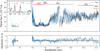 |
Fig. 1 Combined observation spectrum of WISE 1738 from instruments HST/WFC3, Gemini/GNIRS, and MIRI/JWST (scaled to a distance of 9.9 pc). Top : WFC3 (J and H bands, red), GNIRS (Y, J, H and K bands, black), and MIRI (black) observations xobs, overlaid with the simulated noiseless spectrum f(θ) associated with the most probable parameters from the posterior. Bottom : residuals of the sample normalized by the inflated standard deviation of the noise distribution for each spectral channel. |
2.3 Gemini/GNIRS spectrum
A higher-resolution near infrared spectrum for WISE 1738 was also obtained from the data obtained by the Gemini North telescope using the GNIRS, at a resolving power of approximately 2800, via the program GN-2014A-Q-64 (Elias et al. 2006b). Further information on this can be found in the work by Leggett et al. (2016b). The spectrum covers a wavelength range of 0.993-1.087 μm, 1.191-1.305 μm, 1.589-1.631 μm and 1.985-2.175 μm, i.e., spanning the Y, J, H, and K bands. For the retrievals in this work, this spectrum is re-binned down to a resolution λ/Δλ = 1000 to match the default resolution of petitRADTRANS.
3 Atmospheric radiative transfer model
The atmospheric forward model f used in this study was implemented using petitRADTRANS (version 2.6.3) along with a noise model to account for the measurement noise. petitRADTRANS (Mollière et al. 2019) is a one-dimensional radiative transfer model that is used to calculate the emission and transmission spectra for exoplanets with cloudy and cloud-free atmospheres. This model simulates a single atmospheric column consisting of multiple distinct pressure layers, with temperatures determined by a freely parameterized thermal profile. The layers include various opacity sources dispersed throughout the column, and are incorporated into the radiative transfer equations. Here we adopted this setup to model a cloud-free atmosphere. This is because, although Line et al. (2017) found an alkali depletion trend consistent with the theoretical trend of Na2S and KCl condensation curves intersecting with the thermal profile, previous studies on late-T (Line et al. 2017) and early Y dwarfs (Zalesky et al. 2019) have found no strong evidence for the presence of optically thick Na2S and KCl clouds. This is contrary to expectations for cooler brown dwarfs (Kirkpatrick 2005). Further, so far Y dwarfs have been well characterized without the need for water or ammonia clouds (Kühnle et al. 2025; Barrado et al. 2023; Zalesky et al. 2019).
The cloud-free model was parameterized using 26 parameters, denoted as θ. The P- T profile was calculated on a pressure grid containing various levels between 10−6 and 1000 bar. Within this grid, 10 nodes were equidistantly defined in log-space. The temperature at the bottom-most node was set as a free parameter Tbottom, such that it can take any value uniformly distributed between 100 to 9000 K. The temperature at each upper node was calculated as a parameterized fraction uniformly distributed between 0.2-1.0 of the temperature at the node immediately below it. These 9 node fractions were defined as Tnodes[i-ix]. Once the temperatures at all the nodes were calculated, the entire profile was constructed by quadratically interpolating between them.
The primary absorber species typical in Y-dwarf atmospheres with an effective temperature (Teff) of approximately 400 K - such as CH4, H2O, H2S, CO2, CO, and NH3 - were considered (see Figure 5 in Leggett et al. 2015), along with the isotopolog 15NH3 (Barrado et al. 2023). Our model additionally incorporated HCN and PH3 (Visscher et al. 2006; Zahnle & Marley 2014) and TiO and VO, the latter two of which are notably present in higher temperature brown dwarfs, such as late-type M dwarfs (Kirkpatrick et al. 1999). Sources of continuum opacity such as H2-H2 and He-H2 collision-induced absorption bands were also considered. The logarithm (of base 10) of the abundance of each opacity species, expressed as mass fractions, was treated as a free parameter.
Brown dwarf atmospheres are expected to exhibit significant turbulence, affecting species such as CH4, CO, CO2, N2, and NH3 (-e.g., Noll et al. 1997; Saumon et al. 2000; Golimowski et al. 2004; Leggett et al. 2007; Visscher & Moses 2011; Zahnle & Marley 2014). Further, Mukherjee et al. (2022) suggest (log) mixing values between 6-7 for brown dwarfs between 400-500 K. Consequently, we assumed the considered abundances remain constant throughout the pressure column, with values (in log 10 units) uniformly distributed between −10 and 0. We note that recent studies such as Rowland et al. (2023) have demonstrated that this approach may oversimplify atmospheric complexities, potentially leading to inaccurate retrievals of gravity, metallicity, and C/O ratios, irrespective of the parameterization of the P-T profile. This could be incorporated into future retrievals that utilize broad wavelength ranges enabled by combined approaches.
The spectra were calculated with the radiative transfer routines implemented in petitRADTRANS. The planet mass Mp and radius Rp were also considered to be free parameters and used to calculate the emission flux. Measurement noise e was added to the generated flux f(θ) such that the simulator output is given as x = f (θ) + ε, where ε is drawn from a Gaussian noise distribution  defined uniquely for each instrument. Here, ε ∈ RL represents a vector containing random noise instances in each wavelength bin, where L is the combined spectral length of the WFC3+GNIRS+MIRI observations. To account for the random instrument effects and the missing forward model physics, an additional scaling factor, b, was added to inflate the standard deviation on the noise measured for each instrument such that the total error s is given by
  (Line et al. 2015). The free parameters bw, bg and bm pertaining to instruments WFC3, GNIRS, and MIRI instruments, respectively, were set to take values uniformly distributed in the range of [−17, −11), [−17, −11) and [−15, −7). These parameter ranges scale the maximum standard deviations of their respective instruments by factors of 1.35, 1.1, and 33 times, respectively. A lower prior range chosen for the WFC3 and GNIRS than for the MIRI b factors was motivated empirically based on our previous retrievals on this source that consistently prefer an insignificant increase in the noise scaling over the near-infrared range, potentially due to relatively robust and well-understood (preliminary) error bars on these older instruments. The prior distribution chosen in the case of a cloud-free model was a 26-dimensional multivariate uniform distribution p(θ) with physically motivated ranges for each parameter listed in Table 1.
4 Atmospheric retrieval
We performed the atmospheric retrieval using a simulationbased inference algorithm called neural posterior estimation (NPE, Vasist et al. 2023). In NPE, a neural network-based model called a conditional normalizing flow is trained to estimate the Bayesian posterior distribution p(θ|x) over the model parameters θ given the observation x (see Vasist et al. (2023) for further details on the setup). The training phase included sampling from the prior distribution p(θ) over the model parameters and passing it through an atmospheric simulator p(x|θ) (forward model + noise model) in order to generate noisy spectral simulations. These simulations were compressed in an embedding network, to avoid overfitting by memorization, and were used to train the normalizing flow to generate a conditional probability distribution pφ(θ|x). During inference, the trained normalizing flow conditioned on an observation xobs was used to obtain an approximation of the posterior distribution.
The training set consisted of approximately 3.7 million pairs of parameters and spectra (θ, f (θ)), providing around 1.8 value points per dimension if one were to use a regular 26-dimensional grid. The sample pairs in this training set were split into 90%, 9%, and 1% for training, validation, and testing respectively. The training set included combined simulations of the near-infrared and the mid-infrared wavelengths.
For the training set, atmospheric models between the wavelength ranges of 0.98-2.2 μm in the near-infrared and 4.9-18 μm in the mid-infrared were first simulated to match the default wavelength spacing of λ/Δλ = 1000 in petitRADTRANS. Simulated GNIRS and MIRI spectra kept this default spacing for their respective wavelengths. However, the simulated spectrum for WFC3 wavelengths was convolved to the WFC3 spectral resolution and re-binned to a spacing of 130. To generate the GNIRS component of the training set, the NIR spectrum was masked to match the re-binned GNIRS observations. Similarly, the mid-infrared spectrum was generated to match the MIRI observations. WFC3 and GNIRS have some overlapping coverage in the near-infrared region, although they have different wavelength spacings. All three component spectra were combined to generate the training set. The simulations took around 3200 CPU hours.
During training, random noise realizations were added on-the-fly to the simulated spectra in the training set, to obtain simulated observations x = f (θ) + e. These joint pairs of noisy simulations and their corresponding model parameters were input into the normalizing flow. In each forward pass, the posterior log-density log pφ(θ|x) was computed, where φ is the set of weights of the neural flow network, and the loss function  on φ was minimized over the whole training set (θ, x) (Papamakarios et al. 2021). Hyper-parameter tuning was performed by conducting 128 parallel runs, each with a configuration randomly chosen from a uniform grid (see Appendix A) over all the hyper-parameters. The run leading to lower validation loss and/or more stable training across all atmospheric models was preferred. Each hyper-parameter run took around 24 hours. The time taken to train the posterior estimator pφ(θ|x) was approximately 5.8 hours. Sampling 20469 times from the normalizing flow (i.e., the posterior estimate) took approximately 1 minute on average. Therefore, the total time required to perform a single retrieval, including the overhead cost of dataset generation, hyper-parameter tuning, and training, was approximately 30 hours. The technical details of the architecture of the normalizing flow, hyper-parameter tuning, and the training procedure are provided in Appendix B.
Prior distribution for the 26 model parameters.
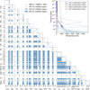 |
Fig. 2 Cloud-free retrieval results using neural posterior estimation on the WISE 1738 spectra. The corner plot shows the full 1D and 2D marginal posterior distributions obtained for the WISE 1738 observations xobs, WFC3+GNIRS+MIRI spectra. The top right figure shows the posterior distribution of the P-T profile. The profile also has the emission contribution function overlaid on top, in shades of white highlighting visibility. The equilibrium state water ice, ammonia, metal chloride and sulfide condensation curves are plotted along the profile in blue, purple, red, and green, respectively for solar metallicity [M/H] and C/O ratio. |
5 Retrieval results
The results of the NPE retrievals on the combined WFC3+GNIRS+MIRI spectral observations xobs of WISE 1738 are presented in the form of 1D and 2D marginal posterior distributions in Fig. 2. These were approximated by extensively sampling from the estimated joint posterior distribution by means of forward passes through the trained normalizing flow. These samples were then used to construct the 68.3%, 95.5%, and 99.7% credible regions of the P-T profile. Along with the constrained parameters, we also show the plot of the derived (i.e., not retrieved) posterior distributions of the 14NH3/15NH3 ratio and log g. The figure also includes the posterior distribution of the P-T profile, shown in the inset. The emission contribution function is overlaid on top of the P-T profile in dashed lines, brightly highlighting the regions of the atmosphere that are probed by the observations. It also includes the equilibrium state water ice, ammonia, metal chloride, and sulfide condensation curves (Lodders & Fegley 2006) in blue, purple, red, and green, respectively. From the plot, it can be seen that the profile is narrower in regions outside the contribution function, and this is due to a more confident prior predictive distribution over those regions, due to the prior’s enforcement of smoother profiles across its space on each temperature node. Further, it can be seen that the water condensation curve intersects with the P-T profile above the upper limit of the probed photosphere, and the metal chloride and sulfide clouds intersect it within the near-infrared photosphere below.
We obtained clear constraints on the abundances of H2O, CO2, CO, CH4, and NH3. All the constrained abundance values are documented in Table 2. We identified upper bounds on 15NH3, PH3, H2S, HCN, TiO, and VO with their 3σ limits −5.68, −5.31, −2.50, −6.15, −6.08, and −8.00 respectively, implying a non-robust detection (Line et al. 2015, 2017). The 3σ limits were computed as the 99.85% upper percentile corresponding to a symmetric 99.7% interval. We also observed that the 14NH3/15NH3 ratio was not well constrained and gave a 3σ lower bound of 275. All the retrieved and computed physical parameters are documented in Table 3. The most probable sample from the posterior, and its normalized residuals which are normalized to the inflated standard deviation are displayed in Fig. 1.
We found that the noise scaling factors (or b factors) were barely constrained for the WFC3 and GNIRS spectra. This implies that the retrieval favors no specific values of noise scaling for the two spectra, within the chosen prior range, and suggests that any random effects are well accounted for within the uncertainties of other parameters without requiring additional noise adjustments. The drop in marginal values from −12 to −11 was a real effect that persisted even when using a broader prior range. Consequently, with the b factors for WFC3 and GNIRS having an upper bound at −12, it reinforces the robustness of these measurements. However, for MIRI, the error estimates were scaled with a b factor found to be around −9. This scaling factor implies that the uncertainty is approximately 4 times higher in the largest error bar compared to the measured value. A detailed evaluation of the estimated posterior, including both qualitative and quantitative assessments such as coverage, posterior predictive distribution, and the L-C2ST test, is presented in Appendix B.
Retrieved atmospheric (log) abundances as volume mixing ratios.
Summary of previous model fits/retrievals attempting to characterize WISE 1738.
6 Discussion
6.1 Combined retrieval vs near-infrared retrievals
Previous studies, such as those by Cushing et al. (2011); Schneider et al. (2015); Zalesky et al. (2019), used WFC3 data to investigate the atmosphere of WISE 1738 while Leggett et al. (2016a, 2017) used the GNIRS data for their analysis. We combined these near-infrared datasets with mid-infrared observations for the first time. The combined retrieval of the WFC3, GNIRS, and MIRI spectra provides a more comprehensive view of the atmosphere by effectively expanding the range of probed pressure levels. This fills gaps even within the near-infrared wavelength range by considering data at different resolutions/observational conditions. The advantage of combining datasets is demonstrated through a comparative study, where we perform single retrievals on WFC3, GNIRS, and MIRI data separately, as well as a combined retrieval on WFC3, GNIRS, and MIRI data. The results of this comparison are shown in Fig. 3.
The comparison revealed that the abundances of CO, CO2, and 15NH3 are more tightly constrained in the combined retrievals than in those based solely on the near-infrared range. This is discussed in more detail in the following subsections. Additionally, although not significant, we saw a similarly slight improvement in the confidence of constraints on the remaining abundances, suggesting that these features are strong in all datasets and hence easier to constrain. Similarly, the constraints on the P-T profile also improved, with the near-infrared region providing tighter constraints on the deeper atmospheric layers, while the mid-infrared region contributed to tighter constraints in the upper layers. Although we found values of the major opacity species such as H2O, CH4, and NH3 to agree with the constraints from Zalesky et al. (2019), their corresponding uncertainties were difficult to compare due to differences in their setups. However, the retrieved posterior validation tests can be found in Appendix B. Furthermore, we did not include alkalis in our final combined retrievals since we found that the MIRI only retrievals do not offer a bound on them, hence offering no added information about their contents from Zalesky et al. (2019) who obtain a 3σ upper bound at −5.2. The most significant improvement, however, was in the constraints on mass, radius, and surface gravity.
The free retrievals conducted exclusively on the near-infrared spectrum, both in our study and in the work by Zalesky et al. (2019), resulted in higher estimates for mass (40 MJ) and surface gravity (5.5 cm s−2), along with a lower estimate for radius (0.7 RJ). In contrast, the combined retrievals resulted in lower masses and gravities and larger radii that aligned better with the predictions from the evolutionary models (discussed more in Sect. 6.3). To explain this difference, we produced consistency plots across the entire wavelength range (see Figs. B.2, B.3 and B.4 in Appendix B), which revealed that in each case, while retrievals remained consistent within the originally retrieved spectral region, they failed to predict consistent spectra in the extended (not retrieved) regions. This was in contrast with the consistency plot obtained for the combined retrieval in Fig. B.1 which exhibited consistency across the extended wavelength range. The enhanced consistency obtained in the latter case demonstrates how biased our characterizations can become when data coverage is limited. It also suggests that when focusing on narrow wavelength regions, multiple competing hypotheses can fit the spectral shape. Therefore, the MIRI spectrum provides critical additional information, enabling improved constraints on these physical parameters. These findings highlight the necessity of incorporating broader datasets to achieve accurate characterizations of brown dwarfs.
Interestingly in the combined retrievals, while the normalized residuals of the consistency plot in Fig. B.1 are found to be centered around the horizontal black line at zero within the 1-10 μm wavelength range, we observed a slight offset above the zero line in the 10-16 μm range. This offset was not observed in retrievals performed exclusively on each individual dataset as shown in the Figs. B.2, B.3 and B.4. Although not significant, this suggests a challenge in reconciling the near-infrared and MIRI spectra, which may stem from either systematic noise effects that are not accounted for in the data calibration, or the absence of a more comprehensive forward model that accounts not only for bulk chemical processes but also for localized chemistry. One such instance is the deep atmospheric dynamics driven by fingering convection under dis-equilibrium chemistry, which can cause compositional gradients to impact the different regions of the spectrum differently, as discussed by Tremblin et al. (2015). Local effects become increasingly important while analyzing such long spectral wavelength ranges that provide deeper insights into larger parts of the atmosphere. Alternatively, the slight discrepancy could arise from an unknown process not accounted for in the forward models, such as a missing opacity source deeper in the atmosphere (Morley et al. 2018; Beiler et al. 2024).
To this effect, we performed tests including water and patchy metal chloride and sulfide clouds. However, while the latter were not constrained, even though from photometric measurements they were suspected to cause the 5% and 30% variability seen in the near-infrared region (Leggett et al. 2015), the water clouds were broadly constrained but were not only not statistically preferred over the cloud-free retrievals, but they also did not account for this difference. However, the lack of constraints on the patchy metal sulfide and chloride clouds, and their condensation curves suggests that they could be formed above the near-infrared photosphere where we do not probe. Additionally, the discrepancy could also be the models attempting to adjust for variations in the temperature continuum slopes.
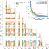 |
Fig. 3 Comparing individual and combined spectral retrievals of WISE 1738 across different wavelength regions. The corner plot shows 1D and 2D marginal posterior distributions obtained for the WFC3, GNIRS, and MIRI spectrum along with the combined WFC3+GNIRS+MIRI spectra. The top right figure illustrates the posterior distribution of the P – T profile of the combined retrieval, while also highlighting the 99.7% credible intervals of the three independent retrievals. |
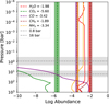 |
Fig. 4 Comparing chemical equilibrium abundances with retrieved values. The plot compares equilibrium chemistry abundance for molecules used in the retrievals (shown in dashed lines, including 1σ uncertainties as colored bars), setup within an atmosphere with C/O = 1.35 and [M/H] = 0.34 (in solid lines), calculated using the retrieved most probable P-T profile. The molecular abundances are in units of mass fractions. The plot includes key opacity-contributing species: H2O (red), CO2 (green), CO (purple), CH4 (brown), and NH3 (orange). The gray regions are the estimated 1σ of the emission contribution functions for the MIRI probed photosphere (at the top) and the near-infrared probed photosphere (at the bottom). |
6.2 Disequilibrium chemistry
Elemental abundances in sub-stellar objects are key to understanding their evolutionary history, as they govern atmospheric opacity and cooling rates (Burrows et al. 2001). These abundance patterns suggest either star-like formation by gravitational collapse or planet-like formation through gravitational instability, situating the sub-stellar brown dwarfs in the gap between higher-mass stars and lower-mass planets. Unlike stars, which directly reveal atomic abundances, the cooler atmospheres of brown dwarfs exhibit molecular abundances that can be used to determine elemental compositions. Additionally, molecular abundances not only reflect the atmospheric chemistry but also the dynamics at play within these atmospheres. In some instances, these molecular abundances are sensitive to equilibrium condensate rainout and vertical disequilibrium mixing (Burrows et al. 2001; Sharp & Burrows 2007). In Fig. 4, we show a comparison between the retrieved molecular abundances, expressed as mass mixing ratios, for the key opacity-contributing species H2O, CO2, CO, CH4, and NH3, and the easyCHEM chemical equilibrium calculations for an atmosphere with a composition identical to the retrieval of WISE 1738, having a C/O = 1.35 and [M/H] = 0.34, tabulated in petitRADTRANS (see, Mollière et al. 2017; Lei & Mollière 2025), in order to gain insights into the atmospheric dynamics of WISE 1738.
The retrievals constrained the abundances for CO and CO2, even though their chemical equilibrium abundances were expected to be depleted at pressures lower than 1 bar. The fact that these species could be constrained to values higher than that expected for chemical equilibrium, using data from a higher photospheric region (illuminated by the MIRI spectrum), while remaining unconstrained in the near-infrared retrievals (unexpected under chemical equilibrium), provides clear evidence of disequilibrium mixing. This is explored in detail by Beiler et al. (2024), who investigated the over-abundance of CO2 in brown dwarf atmospheres and suggested vertical mixing as a reason for this enhancement, despite an expectation to be quenched. These significant deviations suggest that additional processes, such as vertical mixing or chemical kinetics, need to be incorporated to fully explain the observed abundances with self-consistent models.
In contrast, while the retrieved opacity of CH4 aligned well with equilibrium values consistent with previous studies (Burrows & Sharp 1999; Sharp & Burrows 2007), H2O was retrieved to have a higher value. However, the retrieved abundance of NH3 was lower than its equilibrium value in the MIRI probed photosphere, which was likely depleted due to quenching (Zahnle & Marley 2014), but was consistent with the near-infrared probed photosphere lower in the atmosphere. Consistency with equilibrium abundance we found in CH4 confirms a constant abundance profile for the molecule within the dis-equilibrium state of the atmosphere.
Additionally, we calculated a ratio of 14NH3/15NH3 which has recently been proposed as a new tracer for formation history (Barrado et al. 2023). Our measurement, which was non-robustly constrained with a 3σ lower bound value of 275, largely overlapped with the range found for WISE 1828 ( ) and the solar system. However, it also included much lower estimates, aligning more closely with the estimate of 332-49 for WISE 0855 reported by Kühnle et al. (2025) and the ISM. Such broad values failed to identify core collapse as the formation pathway expected for brown dwarfs, as opposed to core accretion of exoplanets. Additional measurements of other isotopologs in the atmosphere of WISE 1738 could help determine their reliability as a diagnostic for tracing formation history.
6.3 Evolution of WISE 1738
We estimated the effective temperature of WISE 1738. This calculation relied on the bolometric fluxes over a broad wavelength range of 0.8 to 50 μm, derived from the retrieved posterior. Assuming a distance of 7.34 pc (Martin et al. 2018) and the retrieved radius posterior, the effective temperature was determined to be  K, which is in agreement with previous estimates in Table 3. Additionally, the log g was calculated using the retrieved values for mass and radius, yielding a result of
  .
.
The evolutionary models presented by Saumon & Marley (2008) and Marley et al. (2021) suggest that a brown dwarf with an effective temperature of approximately 400 K and a log g between 4.1 and 4.7 cm s−2 would have a mass in the range of 6-20 MJ, a radius between 0.97 and 1.1 RJ, with a bolometric luminosity log L/L⊙ between −6 and −7. The retrieved mass of  , a radius of 1.14RJ, and bolometric luminosity of
  align reasonably well with these theoretical predictions, supporting consistency between observed and modeled parameters. Further, we estimated an age spanning 1-4 Gyr using the evolutionary model from Marley et al. (2021), which is consistent with the rotation period of 6 hours measured for WISE 1738 (Leggett et al. 2016a), as brown dwarfs are expected to spin faster as they age (Bouvier et al. 2014).
6.4 C/O and metallicty
We determined the carbon-to-oxygen (C/O) ratio to be  and metallicity [M/H] to be
  , under the considered atmospheric model, assuming no oxygen sequestration in the atmosphere. However, the derived atmospheric abundances may not reflect the true chemical composition of the atmosphere because some chemical elements can be used up in cloud particles and/or are removed from the atmosphere due to rainout. Atmospheric oxygen is typically depleted by 20-30% relative to intrinsic values due to sequestration in condensates, with the extent of depletion depending on the intrinsic metallicity and C/O ratio (Line et al. 2015). This process increases the atmospheric C/O ratio while reducing the overall atmospheric metallicity, as oxygen is a dominant metal. We considered this by specifically accounting for enstatite and forsterite condensation (Fegley & Lodders 1994) by adjusting the abundances of oxygenbearing molecules by a factor of 1.3, following the approach in Zalesky et al. (2019). This adjustment was equivalent to the removal of 3.28 oxygen atoms for every silicon atom (Burrows & Sharp 1999). Incorporating this sequestration, we recalculated the C/O ratio and metallicity [M/H] as
  and
and  , respectively. These values lie within 2σ and 4σ of solar values, respectively.
Such super-solar C/O ratios and metallicity have been observed in late T-dwarfs, as reported by Line et al. (2017); Zalesky et al. (2019). This ratio also aligns with the upper range of the local FGK population, which extends to a C/O ratio and metallicity up to values 1.4 and 0.6, respectively (Zalesky et al. 2019; Hinkel et al. 2014).
Brown dwarfs are thought to form via gravitational collapse that should result in near-solar C/O ratios and metallicity. However, if it is formed around a star and ejected, this could change. It is interesting to note that Pascucci et al. (2013) and more recently Tabone et al. (2023); Arabhavi et al. (2024), find the inner disk to be carbon-rich with molecules such as C2H2, HCN, C6H6, CO2, HC3N, C2H6, C3H4, C4H2, and CH4 dominating the disk with little traces of H2O (Arabhavi et al. 2025), suggesting that such values could be an artifact of formation. However, further understanding of oxygen sequestration processes and formation scenarios is necessary to explain such a high C/O ratio and metallicity.
6.5 Comparison with grid models
We compared the retrieved P-T profile posterior of WISE 1738 to the closest 1D self-consistent atmospheric models in terms of bulk properties such as effective temperature, surface gravity, and metallicity. For this comparison, we used models from grids by Lacy & Burrows (2023) and the Sonora Elf Owl (Mukherjee et al. 2024). We chose these models since they embody disequilibrium chemistry and clouds suited for WISE 1738’s expected temperature range.
These two sets of grids were modeled with radiative-convective equilibrium, and equilibrium chemistry or vertical mixing-induced disequilibrium chemistry in Y dwarf atmospheres used here. Lacy & Burrows (2023) uses coolTLUSTY Burrows et al. (2008); Hubeny & Lanz (1995); Sudarsky et al. (2005) to generate models spanning various ranges of effective temperatures, metallicities and surface gravities2. Additionally, Sonora Elf Owl spans sub-solar to super-solar atmospheric Carbon-to-Oxygen ratios and vertical eddy diffusion coefficients and uses PICASO (Batalha et al. 2019; Mukherjee et al. 2023) to generate the models3. Both of these models include both (water ice) cloudy and clear cases.
6 models from Lacy & Burrows (2023) were chosen for comparison. These included both clear and cloudy atmospheres with equilibrium and dis-equilibrium chemistry. In each case, the models had a log g of 4.5, Teff of 400 K and a metallicity of 0.316. Additionally, the cloudy models used, included two types of tapering of cloud opacity along the height of the atmosphere (see Equation (2) of Lacy & Burrows (2023)). These are denoted by the naming convention AEE and E which represent weak and strong tapering factors with values 2 and 6 respectively. In each case, the model cloud particle size used was 10 μm. These models are labeled as AEE10 and E10 respectively. For models with vertical mixing, a mixing coefficient, log kzz, of value 6 was used. Similarly, 5 Sonora Elf models were chosen for comparison. These included log g of 4.5, Teff of 400 K and a metallicity of 0.5, along with various values of the mixing coefficient, log kzz, between 2 and 9.
These grid comparisons are plotted in Figure 5. Firstly, we found more variation between grids than within each grid, which speaks about the impact of the differing treatment of the physical processes solved in each case. Further, we found that Sonora Elf Owl models are compatible with the posterior distribution of WISE 1738, while the Lacy models are not for all variations of configurations chosen.
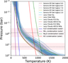 |
Fig. 5 Comparison of the P-T posterior of WISE 1738 with the nearest possible grid model (in terms of Teff, log g, composition, etc) from Lacy & Burrows (2023) and Sonora Elf Owl (Mukherjee et al. 2024), for several clear and cloudy, and equilibrium and dis-equilibrium conditions. The pink regions are the estimated 1σ of the emission contribution functions for the MIRI probed photosphere (at the top) and the near-infrared probed photosphere (at the bottom). The equilibrium state water ice, ammonia, metal chloride and sulfide condensation curves are plotted along the profile in blue, purple, red, and green respectively for solar metallicity and C/O ratio. |
7 Conclusion
Y dwarfs are among the coldest and least luminous brown dwarfs, offering unique opportunities to explore the thermal, chemical, and evolutionary properties of cool sub-stellar objects. Their predominantly cloud-free atmospheres and spectra shaped by strong water vapor, methane, and ammonia absorption, provide a large spectral dynamic range crucial for probing their pressure-temperature (P-T) profiles (e.g., Marley et al. 1996; Line et al. 2015). These objects serve as ideal laboratories for studying key atmospheric species such as H2O, CH4, CO, and NH3 along with its isotopolog 15NH3, which dominate the carbon and oxygen chemistry. This enables a precise determination of metallicity and carbon-to-oxygen (C/O) ratios, which are keys to link atmospheric compositions to evolutionary models.
While previous retrievals have primarily focused on nearinfrared wavelengths, the inclusion of mid-infrared data from the Mid-Infrared Instrument of the James-Webb Space Telescope allowed us to probe higher in these atmospheres, offering improved constraints on physical parameters like surface gravity, radius, mass, luminosity, and unveiling dis-equilibrium chemistry by more accurately constraining chemical abundances. In this study, we built a comprehensive understanding of the Y dwarf WISE 1738 by retrieving its P-T profile, chemical abundances (including an isotolpolog), comparing these findings to evolutionary models, and setting the stage for future investigations into complex atmospheric processes and cloud formation.
We performed atmospheric retrievals using neural posterior estimation on the combined spectral data from WFC3+GNIRS+MIRI observations. To estimate their posterior distribution, we trained a normalizing flow based on the amortized variational inference algorithm, using the atmospheric emission models generated with the simulator petitRADTRANS. By combining retrievals over an extended wavelength range, we demonstrated a reduction in uncertainty in the retrieved P-T profile and in some molecular abundances, compared to individual retrievals from each observation. We also caution against potential biases in spectral characterization that may arise from using narrower wavelength ranges, highlighting improved consistency between the estimated posterior and the observations when combined spectral data is used instead of individual spectral retrievals. This confirms trends that we have seen in short-wavelength retrievals.
Additionally, we constrained the bulk physical properties of WISE 1738 including mass, radius, surface gravity, and luminosity, with higher accuracy, in agreement with theoretical predictions from evolutionary models. We also estimated the object’s age to be between 1 and 4 Gyr, which is consistent with the fast rotation period of 6 hrs. However, reconciling the nearinfrared and mid-infrared regions proved challenging, suggesting the presence of uncalibrated systematic noise or an unknown process such as local chemistry, a missing opacity source, or intrinsic variability that is not yet accounted for.
In addition to the major opacity species such as CH4, and H2O, we also estimated the abundances of CO2, CO, and the depleted NH3, for the first time on this object. These results provided evidence of disequilibrium chemistry in WISE 1738’s atmosphere due to vertical mixing, as they could not be constrained by the near-infrared data alone, and equilibrium chemistry predicts their depletion below the near-infrared photosphere. This result adds to the evidence of vertical mixing in brown dwarf atmospheres.
We performed grid comparisons with the NPE retrieval. We compared the P-T profile NPE posterior of WISE 1738 with several clear and cloudy, equilibrium and disequilibrium grid models. We found that the choice of grid greatly affects the resulting P-T profiles. Further, we found that the Sonora Elf Owl grid is consistent with the retrieval, whereas the Lacy grid is not, irrespective of the type of atmosphere chosen.
Acknowledgements
This project has received funding from the European Research Council (ERC) under the European Union’s Horizon 2020 research and innovation program (grant agreements No. 819155), and from the Wallonia-Brussels Federation (grant for Concerted Research Actions). Computational resources have been provided by the Consortium des Équipements de Calcul Intensif (CÉCI), funded by the Fonds de la Recherche Scientifique de Belgique (F.R.S.-FNRS) under Grant No. 2.5020.11 and by the Walloon Region. JPP acknowledges financial support from the UK Science and Technology Facilities Council, and the UK Space Agency; along with the Spain Ministry of Science, Innovation/State Agency of Research MCIN/AEI/10.13039/501100011033, Grant No. PID2023-150468NB-I00.
Data availability
The MIRI spectrum in Fig. 1 is available at the CDS via https://cdsarc.cds.unistra.fr/viz-bin/cat/J/A+A/703/A70
Appendix A Technical details on NPE
In this work, the normalizing flow is defined as a neural autoregressive flow (NAF, Huang et al. 2018) implemented in the lampe package4. It takes the model parameters and the “context” as inputs. Here, the context includes either spectral simulations from the training set or the observation spectrum, depending on whether one is in the training or the inference phase. The flow outputs an estimate of the posterior distribution pφ(θ|x). The NAF is composed of several transformations parameterized by a neural network. Each transformation network is defined by a monotonic multilayer perceptron (MLP) and a signal network that conditions the MLP. The signal network is an autoregressive conditional function over the model parameters, taking these parameters and the context as input and giving a signal vector that conditions the MLP as the output. The NAF is parameterized by three transformations, each defined by an MLP with five hidden layers of size 512. These MLPs are conditioned on a signal output of length 16, and use Exponential Linear Unit (ELU) activation functions (Clevert et al. 2015).
Before the context is input into the NAF to condition the transformations, it is compressed using an “embedding” network. This network embeds the spectrum such that important features are extracted instead of memorizing the training set, thus preventing overfitting. The embedding network is implemented as a ResidualMLP (or ResMLP), one for each region of the spectrum. The ResidualMLP networks consist of several linear blocks that decrease in size (He et al. 2016). The MIRI embedding network contains 10 residual blocks with dimensions 2 × 512 + 3 × 256 + 5 × 128, whereas the WFC3+GNIRS embedding network contains 15 residual blocks with dimensions 3 × 512 + 5 × 256 + 7 × 128, which are used to compress the length of the input features from (129+305)+1298, to a vector of feature length 8+64. Each of these embedding networks use ELU as their activation functions. The loss function NPEloss is used to optimize the training.
During training, the optimization of the normalizing flow is carried out through a variant of stochastic gradient descent, namely AdamW (Loshchilov & Hutter 2019). The initial learning rate used for training is 10−3, which is halved every time the average loss over the validation set does not improve for 32 continuous epochs, until it hits the value 10−8. This prevents overfitting (Zhang et al. 2023). A weight decay of 10−2 is used for the training. The normalizing flow is trained for a total of 100 epochs, during which 1700 random batches of 1024 and 256 pairs each of (θ, f (θ)) are used from the training sets. The architectural hyper-parameters are adjusted on the validation data.
To arrive at the above architectures, we performed extensive hyper-parameter tuning on the flow, embedding network parameters, and the loss function. For robustness, the twelve best configurations out of the 128 were chosen to perform all the retrievals conducted in this paper. The results from the best model among them are presented here. However, the variation in the results observed between these architectures is minimal. For the flow, we explored different numbers of transforms and hidden layer dimensions in the range of [3,5] and [256,512], respectively. For the embedding network, we tried different numbers of layers in the ResMLP in the range of [10,15] for each instrument, along with different embedding outputs in the range of [4,16] for the WFC3+GNIRS spectra. We explored both the regular NPEloss and the BalancedNPEloss functions to penalize the overconfident posteriors (Delaunoy et al. 2023). We explored different values for the initial learning rate and minimum learning rate in the range of [10−5,10−3] and [10−8,10−5] respectively, and weight decay in the range of [10−2,0]. We analyzed the impact of different schedulers such as ReduceLROnPlateau and CosineAnnealingLR available in PyTorch, which allow dynamic learning rate reduction based on the validation loss, with patience rates between [8,32]. We tried batch sizes between [28,211] and the number of epochs between [27,210].
Similar to Vasist et al. (2023), amongst all the parameters that we tuned, the parameter weight decay between [0,10−2] had the most significant impact on the training. We think this is because of the high variance of the input dataset, where some spectra are six orders of magnitude brighter than the rest. This leads to the skewing of the weights to very high values, which is compensated by weight decay to improve training performance. For more details, we refer to the source code of the experiments5.
Appendix B Diagnostics
The posterior density estimator, trained on simulated data, is subjected to three diagnostic tests to evaluate its validity: the qualitative consistency plot, the coverage test, and the quantitative L-C2ST.
Appendix B.1 Consistency plot
A qualitative test to evaluate the consistency of the approximated posterior with the observation is by comparing the posterior predictive distribution p(x′|x) (Vasist et al. 2023) with it. This represents a distribution of the possible future observations x′, given the current observation x and the model parameters θ. It is calculated as  where p(x′|θ) is the likelihood of the new data given the model parameters, and p(θ|x) is the estimated posterior distribution. The posterior predictive distribution is obtained by sampling parameters from the posterior θ ~ pφ(θ|xobs), and then computing their spectra f(θ) + ε using the simulator (which includes noise). One evaluates the quality of the fit by visually comparing the consistency of the posterior predictive distribution with the observation.
The cloud-free posterior predictive distribution for the WFC3+GNIRS+MIRI spectra is displayed in Fig. B.1. The results indicate that the posterior predictive distribution is well constrained, with the xobs centered well within the noise limit in most wavelengths with a small spread. We also plot the residuals normalized by the inflated error bars across all wavelengths.
Similarly, in Figs. B.2 and B.3, we compare the posterior predictive distributions for the independent posteriors obtained from separate retrievals on the MIRI and GNIRS spectra, each extended to the wavelength range covered by the WFC3+GNIRS+MIRI spectra. The inconsistencies observed in spectral regions not included in the original retrieval highlight potential biases in characterization when data availability is limited.
Appendix B.2 Coverage
Coverage is the probability of the true value of the model parameters appearing in a credible region of the estimated posterior distribution. It evaluates the consistency of the approximated posterior to assess whether it is under or over dispersed on average.
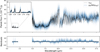 |
Fig. B.1 Top. WFC3+GNIRS+MIRI consistency plot. The posterior predictive distribution |

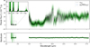 |
Fig. B.2 Top. MIRI consistency plot. Posterior predictive distribution |

The coverage test is conducted by performing numerous retrievals on several simulated noisy spectra from the test set, and comparing their corresponding approximate posterior distributions with their nominal model parameter values. Based on the work by Hermans et al. (2020), the expected coverage probability of the 1 − α highest posterior density regions derived from the estimated posteriors pφ(θ|x) is defined as
![Mathematical equation: \mathbb{E}_{p(\theta,x)}\left[1\left(\theta \in \Theta_{p_\phi(\theta|x)}(1 - \alpha)\right)\right],](/articles/aa/full_html/2025/11/aa54282-25/aa54282-25-eq56.png) (B.1)
(B.1)
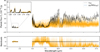 |
Fig. B.3 Top. GNIRS consistency plot. Posterior predictive distribution |

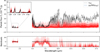 |
Fig. B.4 Top. WFC3 consistency plot. Posterior predictive distribution |

where, 1(∙) is the indicator function, and the function Θpφ(θ|x)(1 − α) yields the 1 − α highest posterior density region of pφ(θ∣x). This is calculated as the percentage of times the nominal parameter values θtest from the test set fall within a specified highest density region (1 − α) of the corresponding estimated posterior pφ(θtest|xtest), where xtest = f(θtest) + ε. The computed coverage probability is plotted along credibility levels ranging between [0,1] on the x axis.
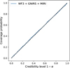 |
Fig. B.5 Coverage plots for cloud-free model posterior estimator. This plot suggests that the estimator is well calibrated. |
Figure B.5 plots the coverage probabilities for our NPE retrieval. Ideally if the posteriors are well calibrated, then θtest should be contained in the 1 − α highest posterior density regions of the approximate posteriors pφ(θtest|xtest) exactly (1 − α)% of the time. If the coverage probability is smaller than the credibility level 1 − α, then this indicates that the posterior estimator is overconfident. On the other hand, if the coverage probability is larger than the credibility level 1 − α, then this indicates that the posterior approximations are conservative. Here, we see that for the retrieval, the coverage plot almost aligns with the ideal case scenario (the dashed diagonal line). The probabilities align closely with a diagonal straight line, indicating well-calibrated posterior approximations.
Given that this test requires several posterior estimations performed on the test set, it cannot be applied to non-amortized techniques; however it is straightforward in NPE. Here amortization is the ability to train the network once over one atmospheric model, and use it to perform retrievals over many observations almost quasi-instantaneously without having to start from scratch, which is a feature of NPE (and some other SBI algorithms).
Appendix B.3 Local classifier two-sample test
Since coverage is a global validation method, it serves as a necessary but not sufficient condition for a valid inference algorithm. A coverage check that fails indicates that the inference is invalid, while passing coverage checks does not guarantee that the posterior estimation is accurate. This is because coverage deals with cumulative probability and does not account for local inconsistencies. This limitation motivates the use of a local validation procedure called the local classifier two-sample test (L-C2ST, Linhart et al. 2024). L-C2ST allows for the local evaluation of a posterior estimator at any given observation. In case of an inconsistency, L-C2ST is also able to graphically show how to improve the estimator.
The test involves training a classifier to distinguish between samples drawn from the true joint distribution p(θ, x) (class 0) and those drawn from the estimated posterior q(θ | x)p(x) (class 1). For a normalizing flow, this translates to learning to differentiate samples from N(0,Im)p(x) (class 0) and  (class 1). The classifier is trained under the null hypothesis, which asserts that the two distributions are indistinguishable. Formally, the null hypothesis under the normalizing flow (NF) is expressed as:

where, xobs is any observation over which one is evaluating the quality of the retrieval.
The classifier is also trained once on the observed data where the training set retains the relationship between variables to account for real-world variability. Finally, the classifier is evaluated on a single observation xobs based on metrics that rely on the L-C2ST statistic. The statistic is the mean squared error (MSE) between 0.5 and the predicted probabilities from the classifier of being in class 0 over the dataset (θobs, xobs).
The first metric is the p-value, which is the proportion of the times the L-C2ST statistic under the null hypothesis is greater than the L-C2ST statistic at the observation xobs. This is computed as the empirical mean over statistics obtained from several trials under the null hypothesis:

where, LC2ST(xobs) is the L-C2ST statistic at the observation xobs,  are the statistics under the null hypothesis, and I(∙) is the indicator function. The distribution under the null hypothesis is called the T-distribution. If the posterior estimate is not close to the true posterior, the classifier will identify a significant difference between the two classes, resulting in higher values of the statistic and hence very small p-values. If this value is less than the assumed significance level, it indicates that the null hypothesis does not hold.
The binary classifier is implemented as an ensemble of 15 Multi-layer Perceptrons (MLP) from scikit-learn. The classifier is initialized with two hidden layers, each having a number of neurons equal to 10 times the number of input features (ndim = 26). The ReLU activation function is used in the hidden layers, and the Adam optimizer is employed to adjust the model’s weights. The training process runs for a maximum of 100 iterations. The classifier is trained on 50k samples from the training set. When trained, the classifier uses back-propagation to minimize the binary cross-entropy loss function, adapting its weights to improve predictions of one of two possible outcomes (-e.g., 0 or 1) based on the input data.
We calculate the p-values for: the estimated posterior for WISE 1738’s spectrum (Observation 3), the most probable simulated observation (Observation 1), and a random sample from the prior (Observation 2). This is illustrated in Fig. B.6. In each case, the T-distribution shown in Fig. B.7 indicates a p-value well within the rejection threshold of 0.05, suggesting that the null hypothesis cannot be rejected. This implies that the estimated posterior for these observations is close to the true posterior.
Next, we present the pp-plots for these observations (see Fig. B.8). The pp-plot, a variation of the coverage plot, helps assess the overall trend of bias or the potential over- or underconfidence of the estimated posterior. For the estimated posterior of WISE 1738’s spectrum and observation 3, the red curve is entirely within the gray confidence region, suggesting that it is neither significantly over-dispersed nor under-dispersed. However, there is a slight rightward bias (a small deviation from the dashed vertical line), indicating that some estimated parameters may be slightly higher than the nominal value. In contrast, Observation 1 shows less bias and is valid.
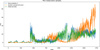 |
Fig. B.6 The three observations for which we evaluate the estimated posterior. |
 |
Fig. B.7 T distribution plot. The p-values are computed as the proportion of the times the L-C2ST statistic under the null hypothesis is greater than the L-C2ST statistic at the observation xobs. |
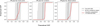 |
Fig. B.8 pp-plot. Cumulative distribution function (CDF) for the three posterior estimates. |
References
- Allard, F., Hauschildt, P. H., Baraffe, I., & Chabrier, G. 1996, ApJ, 465, L123 [NASA ADS] [CrossRef] [Google Scholar]
- Arabhavi, A. M., Kamp, I., Henning, T., et al. 2024, Science, 384, 1086 [NASA ADS] [CrossRef] [Google Scholar]
- Arabhavi, A. M., Kamp, I., Henning, Th., et al. 2025, A&A, 699, A194 [NASA ADS] [CrossRef] [EDP Sciences] [Google Scholar]
- Argyriou, I., Glasse, A., Law, D. R., et al. 2023, A&A, 675, A111 [NASA ADS] [CrossRef] [EDP Sciences] [Google Scholar]
- Barrado, D., Mollière, P., Patapis, P., et al. 2023, Nature, 624, 263 [NASA ADS] [CrossRef] [Google Scholar]
- Batalha, N. E., Marley, M. S., Lewis, N. K., & Fortney, J. J. 2019, ApJ, 878, 70 [NASA ADS] [CrossRef] [Google Scholar]
- Beichman, C., Gelino, C. R., Kirkpatrick, J. D., et al. 2014, ApJ, 783, 68 [NASA ADS] [CrossRef] [Google Scholar]
- Beiler, S. A., Mukherjee, S., Cushing, M. C., et al. 2024, ApJ, 973, 60 [Google Scholar]
- Bouvier, J., Matt, S. P., Mohanty, S., et al. 2014, in Protostars and Planets VI, eds. H. Beuther, R. S. Klessen, C. P. Dullemond, & T. Henning, 433 [Google Scholar]
- Burrows, A., & Sharp, C. M. 1999, ApJ, 512, 843 [NASA ADS] [CrossRef] [Google Scholar]
- Burrows, A., Hubbard, W. B., Lunine, J. I., & Liebert, J. 2001, Rev. Mod. Phys., 73, 719 [Google Scholar]
- Burrows, A., Ibgui, L., & Hubeny, I. 2008, ApJ, 682, 1277 [NASA ADS] [CrossRef] [Google Scholar]
- Bushouse, H., Eisenhamer, J., Dencheva, N., et al. 2023, JWST Calibration Pipeline [Google Scholar]
- Clevert, D.-A., Unterthiner, T., & Hochreiter, S. 2015, arXiv e-prints [arXiv:1511.87289] [Google Scholar]
- Cushing, M. C., Kirkpatrick, J. D., Gelino, C. R., et al. 2011, ApJ, 743, 50 [Google Scholar]
- Delaunoy, A., Miller, B. K., Forré, P., Weniger, C., & Louppe, G. 2023, in Fifth Symposium on Advances in Approximate Bayesian Inference [Google Scholar]
- Elias, J. H., Joyce, R. R., Liang, M., et al. 2006a, in Ground-based and Airborne Instrumentation for Astronomy, 6269, eds. I. S. McLean, & M. Iye, International Society for Optics and Photonics (SPIE), 62694C [Google Scholar]
- Elias, J. H., Rodgers, B., Joyce, R. R., et al. 2006b, in Ground-based and Airborne Instrumentation for Astronomy, 6269, SPIE, 374 [Google Scholar]
- Fegley, Jr., B., & Lodders, K. 1994, Icarus, 110, 117 [NASA ADS] [CrossRef] [Google Scholar]
- Golimowski, D. A., Leggett, S. K., Marley, M. S., et al. 2004, AJ, 127, 3516 [Google Scholar]
- He, K., Zhang, X., Ren, S., & Sun, J. 2016, in Proceedings of the IEEE Conference on Computer Vision and Pattern Recognition, 770 [Google Scholar]
- Hermans, J., Begy, V., & Louppe, G. 2020, in International Conference on Machine Learning, PMLR, 4239 [Google Scholar]
- Hinkel, N. R., Timmes, F. X., Young, P. A., Pagano, M. D., & Turnbull, M. C. 2014, AJ, 148, 54 [NASA ADS] [CrossRef] [Google Scholar]
- Huang, C.-W., Krueger, D., Lacoste, A., & Courville, A. 2018, in International Conference on Machine Learning, PMLR, 2078 [Google Scholar]
- Hubeny, I., & Lanz, T. 1995, ApJ, 439, 875 [Google Scholar]
- Kimble, R. A., MacKenty, J. W., O’Connell, R. W., & Townsend, J. A. 2008, in Space Telescopes and Instrumentation 2008: Optical, Infrared, and Millimeter, 7010, eds. J. M. Oschmann, Jr., M. W. M. de Graauw, & H. A. MacEwen, International Society for Optics and Photonics (SPIE), 70101E [Google Scholar]
- Kirkpatrick, J. D. 2005, Annu. Rev. Astron. Astrophys., 43, 195 [Google Scholar]
- Kirkpatrick, J. D., Reid, I. N., Liebert, J., et al. 1999, ApJ, 519, 802 [NASA ADS] [CrossRef] [Google Scholar]
- Kirkpatrick, J. D., Cushing, M. C., Gelino, C. R., et al. 2011, ApJS, 197, 19 [NASA ADS] [CrossRef] [Google Scholar]
- Kirkpatrick, J. D., Martin, E. C., Smart, R. L., et al. 2019, ApJS, 240, 19 [NASA ADS] [CrossRef] [Google Scholar]
- Kühnle, H., Patapis, P., Mollière, P., et al. 2025, A&A, 695, A224 [NASA ADS] [CrossRef] [EDP Sciences] [Google Scholar]
- Lacy, B., & Burrows, A. 2023, ApJ, 950, 8 [NASA ADS] [CrossRef] [Google Scholar]
- Leggett, S. K., Saumon, D., Marley, M. S., et al. 2007, ApJ, 655, 1079 [NASA ADS] [CrossRef] [Google Scholar]
- Leggett, S., Morley, C. V., Marley, M., & Saumon, D. 2015, ApJ, 799, 37 [NASA ADS] [CrossRef] [Google Scholar]
- Leggett, S., Cushing, M. C., Hardegree-Ullman, K. K., et al. 2016a, ApJ, 830, 141 [NASA ADS] [CrossRef] [Google Scholar]
- Leggett, S. K., Tremblin, P., Saumon, D., et al. 2016b, ApJ, 824, 2 [Google Scholar]
- Leggett, S., Tremblin, P., Esplin, T., Luhman, K., & Morley, C. V. 2017, ApJ, 842, 118 [NASA ADS] [CrossRef] [Google Scholar]
- Lei, E., & Mollière, P. 2025, easyCHEM: Chemical abundances in exoplanet atmospheres calculator, Astrophysics Source Code Library [record ascl:2506.010] [Google Scholar]
- Line, M. R., Teske, J., Burningham, B., Fortney, J. J., & Marley, M. S. 2015, ApJ, 807, 183 [NASA ADS] [CrossRef] [Google Scholar]
- Line, M. R., Marley, M. S., Liu, M. C., et al. 2017, ApJ, 848, 83 [NASA ADS] [CrossRef] [Google Scholar]
- Linhart, J., Gramfort, A., & Rodrigues, P. 2024, Adv. Neural Inf. Process. Syst., 36 [Google Scholar]
- Lodders, K., & Fegley, Jr., B. 2006, in Astrophysics Update 2, ed. J. W. Mason (Springer), 1 [Google Scholar]
- Loshchilov, I., & Hutter, F. 2019, in International Conference on Learning Representations [Google Scholar]
- Madhusudhan, N., & Seager, S. 2009, ApJ, 707, 24 [NASA ADS] [CrossRef] [Google Scholar]
- Marley, M. S., Saumon, D., Guillot, T., et al. 1996, Science, 272, 1919 [NASA ADS] [CrossRef] [Google Scholar]
- Marley, M. S., Saumon, D., Visscher, C., et al. 2021, ApJ, 920, 85 [NASA ADS] [CrossRef] [Google Scholar]
- Martin, E. C., Kirkpatrick, J. D., Beichman, C. A., et al. 2018, ApJ, 867, 109 [Google Scholar]
- Mollière, P., van Boekel, R., Bouwman, J., et al. 2017, A&A, 600, A10 [Google Scholar]
- Mollière, P., Wardenier, J., van Boekel, R., et al. 2019, A&A, 627, A67 [NASA ADS] [CrossRef] [EDP Sciences] [Google Scholar]
- Morley, C. V., Fortney, J. J., Marley, M. S., et al. 2012, ApJ, 756, 172 [NASA ADS] [CrossRef] [Google Scholar]
- Morley, C. V., Marley, M. S., Fortney, J. J., et al. 2014, ApJ, 787, 78 [Google Scholar]
- Morley, C. V., Skemer, A. J., Allers, K. N., et al. 2018, ApJ, 858, 97 [Google Scholar]
- Mukherjee, S., Fortney, J. J., Batalha, N. E., et al. 2022, ApJ, 938, 107 [NASA ADS] [CrossRef] [Google Scholar]
- Mukherjee, S., Batalha, N. E., Fortney, J. J., & Marley, M. S. 2023, ApJ, 942, 71 [NASA ADS] [CrossRef] [Google Scholar]
- Mukherjee, S., Fortney, J. J., Morley, C. V., et al. 2024, ApJ, 963, 73 [NASA ADS] [CrossRef] [Google Scholar]
- Noll, K. S., Geballe, T. R., & Marley, M. S. 1997, ApJ, 489, L87 [NASA ADS] [CrossRef] [Google Scholar]
- Papamakarios, G., Nalisnick, E. T., Rezende, D. J., Mohamed, S., & Lakshminarayanan, B. 2021, J. Mach. Learn. Res., 22, 1 [Google Scholar]
- Pascucci, I., Herczeg, G., Carr, J. S., & Bruderer, S. 2013, ApJ, 779, 178 [NASA ADS] [CrossRef] [Google Scholar]
- Phillips, M. W., Tremblin, P., Baraffe, I., et al. 2020, A&A, 637, A38 [NASA ADS] [CrossRef] [EDP Sciences] [Google Scholar]
- Rowland, M. J., Morley, C. V., & Line, M. R. 2023, ApJ, 947, 6 [NASA ADS] [CrossRef] [Google Scholar]
- Saumon, D., & Marley, M. S. 2008, ApJ, 689, 1327 [Google Scholar]
- Saumon, D., Geballe, T. R., Leggett, S. K., et al. 2000, ApJ, 541, 374 [NASA ADS] [CrossRef] [Google Scholar]
- Saumon, D., Marley, M. S., Abel, M., Frommhold, L., & Freedman, R. S. 2012, ApJ, 750, 74 [Google Scholar]
- Schneider, A. C., Cushing, M. C., Kirkpatrick, J. D., et al. 2015, ApJ, 804, 92 [Google Scholar]
- Sharp, C. M., & Burrows, A. 2007, ApJS, 168, 140 [NASA ADS] [CrossRef] [Google Scholar]
- Sudarsky, D., Burrows, A., Hubeny, I., & Li, A. 2005, ApJ, 627, 520 [NASA ADS] [CrossRef] [Google Scholar]
- Tabone, B., Bettoni, G., van Dishoeck, E. F., et al. 2023, Nature, 7, 805 [Google Scholar]
- Tremblin, P., Amundsen, D. S., Mourier, P., et al. 2015, ApJ, 804, L17 [CrossRef] [Google Scholar]
- Tsuji, T., Ohnaka, K., Aoki, W., & Nakajima, T. 1996, A&A, 308, L29 [NASA ADS] [Google Scholar]
- Vasist, M., Rozet, F., Absil, O., et al. 2023, A&A, 672, A147 [NASA ADS] [CrossRef] [EDP Sciences] [Google Scholar]
- Visscher, C., & Moses, J. I. 2011, ApJ, 738, 72 [NASA ADS] [CrossRef] [Google Scholar]
- Visscher, C., Lodders, K., & Bruce Fegley, J. 2006, ApJ, 648, 1181 [NASA ADS] [CrossRef] [Google Scholar]
- Wright, G. S., Wright, D., Goodson, G. B., et al. 2015, PASP, 127, 595 [NASA ADS] [CrossRef] [Google Scholar]
- Wright, G. S., Rieke, G. H., Glasse, A., et al. 2023, PASP, 135, 048003 [NASA ADS] [CrossRef] [Google Scholar]
- Zahnle, K. J., & Marley, M. S. 2014, ApJ, 797, 41 [CrossRef] [Google Scholar]
- Zalesky, J. A., Line, M. R., Schneider, A. C., & Patience, J. 2019, ApJ, 877, 24 [Google Scholar]
- Zhang, A., Lipton, Z. C., Li, M., & Smola, A. J. 2023, Dive into Deep Learning (Cambridge University Press), https://D2L.ai [Google Scholar]
MAST, DOI: 10.17909/vzcg-p593
All Tables
All Figures
|
Fig. 1 Combined observation spectrum of WISE 1738 from instruments HST/WFC3, Gemini/GNIRS, and MIRI/JWST (scaled to a distance of 9.9 pc). Top : WFC3 (J and H bands, red), GNIRS (Y, J, H and K bands, black), and MIRI (black) observations xobs, overlaid with the simulated noiseless spectrum f(θ) associated with the most probable parameters from the posterior. Bottom : residuals of the sample normalized by the inflated standard deviation of the noise distribution for each spectral channel. |
| In the text | |
|
Fig. 2 Cloud-free retrieval results using neural posterior estimation on the WISE 1738 spectra. The corner plot shows the full 1D and 2D marginal posterior distributions obtained for the WISE 1738 observations xobs, WFC3+GNIRS+MIRI spectra. The top right figure shows the posterior distribution of the P-T profile. The profile also has the emission contribution function overlaid on top, in shades of white highlighting visibility. The equilibrium state water ice, ammonia, metal chloride and sulfide condensation curves are plotted along the profile in blue, purple, red, and green, respectively for solar metallicity [M/H] and C/O ratio. |
| In the text | |
|
Fig. 3 Comparing individual and combined spectral retrievals of WISE 1738 across different wavelength regions. The corner plot shows 1D and 2D marginal posterior distributions obtained for the WFC3, GNIRS, and MIRI spectrum along with the combined WFC3+GNIRS+MIRI spectra. The top right figure illustrates the posterior distribution of the P – T profile of the combined retrieval, while also highlighting the 99.7% credible intervals of the three independent retrievals. |
| In the text | |
|
Fig. 4 Comparing chemical equilibrium abundances with retrieved values. The plot compares equilibrium chemistry abundance for molecules used in the retrievals (shown in dashed lines, including 1σ uncertainties as colored bars), setup within an atmosphere with C/O = 1.35 and [M/H] = 0.34 (in solid lines), calculated using the retrieved most probable P-T profile. The molecular abundances are in units of mass fractions. The plot includes key opacity-contributing species: H2O (red), CO2 (green), CO (purple), CH4 (brown), and NH3 (orange). The gray regions are the estimated 1σ of the emission contribution functions for the MIRI probed photosphere (at the top) and the near-infrared probed photosphere (at the bottom). |
| In the text | |
|
Fig. 5 Comparison of the P-T posterior of WISE 1738 with the nearest possible grid model (in terms of Teff, log g, composition, etc) from Lacy & Burrows (2023) and Sonora Elf Owl (Mukherjee et al. 2024), for several clear and cloudy, and equilibrium and dis-equilibrium conditions. The pink regions are the estimated 1σ of the emission contribution functions for the MIRI probed photosphere (at the top) and the near-infrared probed photosphere (at the bottom). The equilibrium state water ice, ammonia, metal chloride and sulfide condensation curves are plotted along the profile in blue, purple, red, and green respectively for solar metallicity and C/O ratio. |
| In the text | |
|
Fig. B.1 Top. WFC3+GNIRS+MIRI consistency plot. The posterior predictive distribution |
| In the text | |
|
Fig. B.2 Top. MIRI consistency plot. Posterior predictive distribution |
| In the text | |
|
Fig. B.3 Top. GNIRS consistency plot. Posterior predictive distribution |
| In the text | |
|
Fig. B.4 Top. WFC3 consistency plot. Posterior predictive distribution |
| In the text | |
|
Fig. B.5 Coverage plots for cloud-free model posterior estimator. This plot suggests that the estimator is well calibrated. |
| In the text | |
|
Fig. B.6 The three observations for which we evaluate the estimated posterior. |
| In the text | |
|
Fig. B.7 T distribution plot. The p-values are computed as the proportion of the times the L-C2ST statistic under the null hypothesis is greater than the L-C2ST statistic at the observation xobs. |
| In the text | |
|
Fig. B.8 pp-plot. Cumulative distribution function (CDF) for the three posterior estimates. |
| In the text | |
Current usage metrics show cumulative count of Article Views (full-text article views including HTML views, PDF and ePub downloads, according to the available data) and Abstracts Views on Vision4Press platform.
Data correspond to usage on the plateform after 2015. The current usage metrics is available 48-96 hours after online publication and is updated daily on week days.
Initial download of the metrics may take a while.