| Issue |
A&A
Volume 703, November 2025
|
|
|---|---|---|
| Article Number | A295 | |
| Number of page(s) | 19 | |
| Section | Extragalactic astronomy | |
| DOI | https://doi.org/10.1051/0004-6361/202554841 | |
| Published online | 26 November 2025 | |
Gas-rich dwarf galaxy multiples in the Apertif H I survey
1
ASTRON, the Netherlands Institute for Radio Astronomy, Oude Hoogeveenseweg 4, 7991 PD Dwingeloo, The Netherlands
2
Kapteyn Astronomical Institute, University of Groningen, PO Box 800 9700 AV Groningen, The Netherlands
3
Department of Space, Earth and Environment, Chalmers University of Technology, Onsala Space Observatory, 43992 Onsala, Sweden
4
INAF – Padova Astronomical Observatory, Vicolo dell’Osservatorio 5, I-35122 Padova, Italy
5
School of Physical Sciences and Nanotechnology, Yachay Tech University, Hacienda San José S/N, 100119 Urcuquí, Ecuador
6
Instituto de Astrofísica de Andalucía (CSIC), Glorieta de la Astronomía s/n, 18008 Granada, Spain
7
Department of Physics, Virginia Polytechnic and State University, Blacksburg, VA 24061-0435, USA
⋆ Corresponding author: This email address is being protected from spambots. You need JavaScript enabled to view it.
Received:
28
March
2025
Accepted:
5
September
2025
Abstract
Context. Dwarf-dwarf galaxy encounters are a key aspect of galaxy evolution as they can ignite or temporarily suppress star formation in dwarfs and can lead to dwarf mergers. However, the frequency and impact of dwarf encounters remain poorly constrained due to limitations in spectroscopic studies, such as surface-brightness incompleteness in optical studies and poor spatial resolution in single-dish neutral hydrogen (H I) surveys.
Aims. We aim to quantify the frequency of isolated gas-rich dwarf galaxy multiples using the untargeted, interferometric Apertif H I survey and study the impact of the interaction on star formation rates of galaxies as a function of the on-sky separation.
Methods. Our parent dwarf sample consists of 2481 gas-rich galaxies with stellar masses in the range ∼106 < M⋆/M⊙ ≲ 5 × 10⁹, for which we identified close companions based on projected separation (rp) and systemic velocity difference (|ΔVsys|). We explored both constant thresholds for rp and |ΔVsys| corresponding to 150 kpc and 150 km s−1 on all galaxies in our sample as well as mass-dependent thresholds based on a stellar-to-halo mass relation.
Results. We find the average number of companions per dwarf in our sample to be 13% (20%) when considering mass-dependent (constant) thresholds. We find that the frequency (∼11.6%) of dwarf companions in the stellar mass regime of 2 × 10⁸ < M⋆/M⊙ < 5 × 10⁹ is three times higher than previously determined from optical spectroscopic studies, highlighting the power of H I for finding dwarf multiples. Furthermore, we find evidence for an increase in star formation rates (SFRs) of close dwarf galaxy pairs of galaxies with similar stellar masses.
Key words: galaxies: dwarf / galaxies: groups: general / galaxies: interactions / galaxies: star formation / galaxies: statistics
© The Authors 2025
 Open Access article, published by EDP Sciences, under the terms of the Creative Commons Attribution License (https://creativecommons.org/licenses/by/4.0), which permits unrestricted use, distribution, and reproduction in any medium, provided the original work is properly cited.
This article is published in open access under the Subscribe to Open model. This email address is being protected from spambots. You need JavaScript enabled to view it. to support open access publication.
1. Introduction
Galaxy interactions play a crucial role in galaxy evolution, for example, by enhancing star formation (e.g., Li et al. 2008; Ellison et al. 2008), tidally disturbing the morphologies of galaxies, and redistributing their gas reservoirs (e.g., Barnes & Hernquist 1992; Schweizer 2000; Holincheck et al. 2016). Furthermore, they can lead to mergers, which are thought to also trigger active galactic nuclei (AGN) (e.g., Satyapal et al. 2014; Goulding et al. 2018; Gao et al. 2020; La Marca et al. 2024; Eróstegui et al. 2025), and to be the main drivers of morphological transformations from disks to spheroidal systems (e.g., Martin et al. 2018). However, even nondisruptive flyby events can significantly impact the properties of galaxies and affect their later secular evolution (e.g., Moore et al. 1996; Martin et al. 2021; Kumar et al. 2021). Hence, determining the frequency of such galaxy encounters and their impact on galaxies across all mass scales provides a direct constraint on galaxy evolution models.
Most observational and theoretical studies have been focused on massive galaxies, studying both the pair fractions (e.g., Yee & Ellingson 1995; Kartaltepe et al. 2007; Duncan et al. 2019) and the impact of interactions on galaxy properties (e.g., Sol Alonso et al. 2006; Ellison et al. 2008; Dillamore et al. 2022). However, due to the shallow potential wells of dwarf galaxies (galaxies with stellar masses M⋆ < 5 × 10⁹ M⊙), interactions likely play an even greater role in their evolutionary pathway as these galaxies are more easily disturbed and take longer to return to equilibrium (e.g., Martin et al. 2021). Yet, dwarf-dwarf encounters remain poorly constrained both in their frequency and influence on galaxy properties. Previous studies have already hinted at a difference in the impact that galaxy interactions have on dwarf galaxies when compared to high-mass galaxies, indicating that interactions can both enhance and temporarily suppress star formation rates (SFRs) of dwarf galaxies (Stierwalt et al. 2015; Kado-Fong et al. 2024; Huang et al. 2025), while only enhancement has been observed in higher-mass systems (e.g., Sol Alonso et al. 2006; Huang et al. 2025). In fact, Huang et al. (2025) suggest that the SFR suppression and enhancement in dwarfs in gas-rich pairs (including both dwarf-dwarf and dwarf–high-mass pairs) depends on the proximity of interacting galaxies, pointing toward a distinctly dominant mechanism in interacting dwarf galaxies, which is likely linked to high gas-fractions and shallow potential wells of dwarfs when compared to high-mass galaxies.
Previous studies on the frequency of dwarf galaxy encounters are primarily based on optical spectroscopic studies with large sky coverage. Using data from the Sloan Digital Sky Survey (SDSS), Sales et al. (2013) investigated how the average number of satellite galaxies varies with the stellar mass of the host. For dwarf host masses (M⋆ ≲ 1010 M⊙), they find that the average number of satellites becomes independent of the host mass and is on the order of a few percent for stellar mass ratios above 1/10. Similarly, Besla et al. (2018) (hereafter B18) studied the frequency of dwarf galaxy multiples found in the SDSS catalog, reporting that ∼4% of dwarfs have a close companion within the stellar mass range of (2 × 10⁸ − 5 × 10⁹) M⊙. By comparing to the Illustris-1 cosmological simulation (Vogelsberger et al. 2014; Nelson et al. 2015), they predict this fraction to increase up to ∼6% in future surveys with improved completeness at these masses. Generally, the frequency of dwarf encounters seems extremely rare, that is, on the order of a few percent.
However, optical spectroscopic studies are inherently limited by fiber collisions (Strauss et al. 2002), which limit the detection of close galaxy pairs, and surface brightness, which preferentially exclude diffuse, low-surface-brightness dwarfs (e.g., Blanton et al. 2005). Galaxy interactions can also significantly change morphologies of dwarf galaxies and potentially lower their surface brightness (e.g., Bennet et al. 2018; Torrealba et al. 2019). On the other hand, by enhancing the SFR, interactions can also increase a dwarf’s surface brightness. Depending on the relative contribution of these two effects in a dwarf-dwarf interaction, optical selection could potentially be biased for or against the detection of the interacting pair when compared to single dwarfs. Hence, due to technical limitations and the aforementioned biases, it is hard to robustly constrain the true number of dwarf galaxy encounters using current optical spectroscopic surveys.
Neutral hydrogen (H I) observations provide an alternative method for finding dwarf galaxies. Dwarfs in the field (isolated from high-mass galaxies) tend to be gas-rich with increasing gas fractions toward lower stellar masses (e.g., Geha et al. 2006; Huang et al. 2012; Catinella et al. 2018). In fact, H I is often the dominant baryonic component of these systems, making H I observations an extremely useful tool for finding dwarf galaxies. The Arecibo Legacy Fast ALFA (ALFALFA) H I survey (Giovanelli et al. 2005), a single dish untargeted H I survey conducted with the Arecibo telescope, has already shown how effective H I observations can be in identifying galaxies missed by optical catalogs (e.g., Cannon et al. 2015; Janowiecki et al. 2015; Leisman et al. 2017). Hence, H I surveys can provide a field dwarf galaxy sample that spans the whole range of dwarf diversity, independently of their stellar content.
Previous large-scale untargeted H I surveys (e.g., HIPASS, Meyer et al. 2004; ALFALFA, Giovanelli et al. 2005; Haynes et al. 2018) relied on single-dish telescopes, which lacked the spatial resolution needed to resolve individual dwarf galaxies in close pairs (e.g., 3.5′ for Arecibo, corresponding to ∼70 kpc at a distance of 70 Mpc; Giovanelli et al. 2005). The recent onset of interferometric, untargeted H I surveys (e.g., Apertif, Adams et al. 2022; MIGHTEE, Jarvis et al. 2017; and WALLABY, Koribalski et al. 2020) are now enabling us to both detect and resolve dwarf galaxy multiples as well as isolated dwarfs, making these surveys an extremely powerful tool for constraining the true frequency of dwarf-dwarf encounters in observations.
In this work we used ∼42% of the total spatial coverage and ∼33% of the total spectral coverage of the Apertif H I survey (Adams et al. 2022; Hess et al., in preparation) to constrain the frequency of dwarf encounters and explore the properties of paired galaxies. Our parent sample contains 2481 gas-rich candidate dwarf galaxies within the stellar mass range of ∼106 − 5 × 10⁹ M⊙. We identified pairs and multiples using projected separation and the difference in their systemic velocities, and compared our findings with previous work based on optical spectroscopy. Furthermore, we explored the SFR dependence on the projected separation of paired dwarfs and made comparisons with previous work on gas-rich paired galaxies.
The paper is structured as follows: In Section 2 we describe the Apertif H I survey and the measurements of properties of Apertif detections. Section 3 describes the selection of the parent dwarf sample and gives an overview of its properties. In Section 4 we present our methodology for identifying dwarf multiples and the isolation criteria. In Section 5 we report the frequency of dwarf multiples found in Apertif and explore the effects of interactions on the star formation activity of paired dwarfs. In Section 6 we compare the frequency of dwarf multiples with an optical study by B18, and the SFRs of paired dwarfs with previous study by Huang et al. (2025). Finally, in Section 7 we draw our conclusions.
2. Data
2.1. Apertif H I data
Apertif (van Cappellen et al. 2022) is a phased-array feed receiver system designed for the Westerbork Synthesis Radio Telescope (WSRT). It increased the field of view of the telescope up to 8 deg2 by producing 40 instantaneous compound beams on the sky. This made WSRT (together with Apertif) a great instrument for conducting a wide area survey across the northern sky.
The Apertif imaging survey (Adams et al. 2022) observed selected areas of the sky with declination above 25°. Each Apertif observation is 11.5 hours, with simultaneous execution of neutral hydrogen (H I) spectral line, continuum and polarization imaging. The H I cubes are produced over the topocentric frequency range 1292.5–1429.3 MHz (Adams et al. 2022) and have spatial resolution of 15″ × 15″/sin δ. The Apertif imaging surveys are split into two tiers: the Apertif Wide-area Extragalactic Survey (AWES) that covers ∼2200 deg2 of the sky with one or two observations per field; and the Medium-Deep Survey (MDS) that targets specific areas of the sky with ∼130 deg2 of coverage and up to 12 observations per field (see Adams et al. 2022).
Spectral line cubes for Apertif data were split into four subsets in spectral dimension for easier data handling. In this work, we focus on a subset, which covers line-of-sight velocities from 424 to 10 170 km s−1 (cube 2; see Adams et al. 2022 for a full description of the cube properties). These cubes were the initial targets for source finding as they provide the maximal number of detections by optimizing sensitivity over the velocity channel width of 7.7 km s−1 (Hess et al., in preparation). We used a subset of this data that covers ∼42% of Apertif spatial footprint, as the source finding on the remaining footprint is still ongoing.
2.2. Apertif H I processing
The H I post-processing workflow is publicly available1 and will be described in a future paper. Here, we provide a brief overview.
Within the Apertif imaging survey footprint, observations of individual fields were co-added with channel-based weights (when multiple observations were available), and the 40 compound beams within individual fields were mosaicked. This ensured the best possible S/N per field and fairly uniform sensitivity within individual fields, thereby maximizing the probability of detecting low H I mass sources. However, the obtained sensitivity varies on larger scales (≳2°; larger than the size of an individual field) due to differing numbers of observations per field and instrumental effects (e.g., continuum subtraction) within the Apertif cubes themselves. As a result of the former, mosaicking of neighboring fields has also not yet been optimized for spectral line source finding. On average, the rms noise level around detected sources corresponds to  mJy beam−1.
Spectral line source finding (see Section 2.3) was performed on the mosaicked data. The candidate sources were vetted to remove continuum artifacts and sidelobes from bright H I sources before cleaning. Cleaning was then performed in the image plane, on a per-compound beam basis, using the Apercal (Adebahr et al. 2022) implementation of Miriad’s clean and restor tasks (Sault et al. 2011). After cleaning, the cleaned compound beams were re-mosaicked, and the mask was applied to the cleaned mosaic to produce advanced data products using the SoFiA Image Pipeline (SIP)2 (Hess et al. 2024).
2.3. The H I source finding
The H I source finding on Apertif cubes (Hess et al., in preparation) was conducted on individual Apertif fields using the SoFiA-2 source finder3 (Serra et al. 2015; Westmeier et al. 2021). SoFiA-2 was run using three spatial kernels with full width at half maximum (FWHM) of: 0, 3, and 6 pixels (corresponding to spatial resolutions of 15″, 23.4″, and 39″); and three boxcar spectral kernels of sizes: 0, 3, and 7 channels (corresponding to spectral resolutions of 7.7 km s−1, 23.2 km s−1, and 54.1 km s−1; Hess et al., in preparation). The mask of each candidate detection was then constructed from pixels that have S/N > 3.8 (threshold obtained by the optimization of true vs. false positive detections) in one or more combinations of spatial and spectral smoothing kernels. The mask was constructed for both positive and negative candidates, whose properties were afterward compared and used to correct for false positives. We used a reliability threshold of 0.65 for this comparison to improve the completeness. Candidates that passed the test and subsequent vetting (see Sect. 2.2) were then cleaned. After cleaning and mosaicking, the pipeline used SIP to produce inspection plots containing a Pan-STARRS 1 image (Chambers et al. 2016) overlaid with H I contours, a total H I intensity map, an S/N map, a velocity map, a position-velocity (PV) slice, and a global spectral profile. These inspection plots were made at the original and 40″ resolution for each source, and both were visually inspected before a source was included in the final source list.
2.4. Distance and H I masses of detected sources
We calculated line-of-sight velocity-based distances using the linear density field model of Valade et al. (2024) provided by the Extragalactic Distance Database (EDD) (Tully et al. 2009; Kourkchi et al. 2020). This model is calibrated on the Cosmicflows-4 (CF4) database of galactic distances (Tully et al. 2023), a compendium of redshift-independent distance measurements for ∼56 000 nearby (D ≲ 500 Mpc) galaxies. We adopted the error estimation procedure from Haubner et al. (2025), corresponding to roughly 12% error on average for the Apertif source list. Flow model-based distances for Apertif detections differ from Hubble distances (assuming H0 = 75 km s−1 Mpc−1, which is compatible with the CF4 measurements) by 7% on average, and up to 31%.
We estimated H I masses of each detection using the following relation (e.g., Kennicutt & Evans 2012):
 (1)
(1)
where FH I is the total H I flux, and D the distance to the galaxy. We assumed a 15% error on FH I coming from the calibration of the flux scale, primary beam correction and mosaicking of Apertif compound beams (Kutkin et al. 2022).
2.5. Stellar properties of Apertif detections
Stellar masses (M⋆) and SFRs of galaxies associated with our H I detections were determined following the approach of Leroy et al. (2019), based on a combination of near-infrared (NIR), mid-infrared (MIR), near-ultraviolet (NUV), and far-ultraviolet (FUV) photometry measurements. As in Marasco et al. (2023, hereafter, M23), we focused on archival, publicly available images from the Wide-field Infrared Survey Explorer (WISE; Wright et al. 2010) in bands W1 (3.4 μm) and W4 (22 μm), from the IRAC 3.6 μm and MIPS 24 μm camera on board the Spitzer Space Telescope (Werner et al. 2004), and from the Galaxy Evolution Explorer (GALEX;Martin et al. 2005) for both UV bands. We briefly summarize our procedure below, and redirect the reader to Section 2 and Appendix A of M23 for further details.
Counterpart identification was done galaxy by galaxy by visual inspection of the moment-0 H I maps overlaid on top of the UV images. For systems that are too faint in UV or that are not covered by the GALEX footprint, we looked for non point-like objects in W1 (or in the IRAC 3.6 μm band, if available) that have a counterpart in W4. We stress that, for low-mass or distant galaxies, the counterpart identification is particularly problematic and the chance of selecting a foreground star is not zero. We dealt with this issue a posteriori by cross-matching the Apertif source list with the stellar catalog from the Gaia DR3 (Vallenari 2023), and by visually inspecting all detections whose photometric centroid is closer than the FWHM of W1 (6.1″) from a Gaia detection. With this, we excluded 138 out of 413 inspected cases. In addition, we visually inspected all the remaining detections for which the measured half-light radius is smaller than 3″ (half of the FWHM of the W1 point spread function) and excluded 23 more detections (out of the 58 inspected cases). Thus, 161 detections (out of 471 visually inspected cases) were flagged as having unreliable stellar measurements in the Apertif source list of 3943 detections. These measurements were not taken into account in the final construction of the parent dwarf galaxy sample (see Sect. 3).
Photometry for the identified sources was done on sky-subtracted images after the automatic removal of contamination from point-like sources such as foreground stars and high-redshift background galaxies. With respect to the original procedure from M23, several steps were automated following approaches from previous software packages; specifically, the determination of the inclination and position angles following SExtractor (Bertin & Arnouts 1996) and the cleaning of the sky region following MORPHOT (Fasano et al. 2012). In short, the “cleaned” image was obtained by comparing the original image to its version rotated by 180°, identifying the pixels for which the residual between the two images is larger than three times the root-mean-square intensity in the surrounding region of the rotated image, and replacing these pixels values with those from the rotated image. Full details on these improvements are provided in Appendix A of Marasco et al. (2025). Additionally, we developed an interactive tool to manually mask bright, extended objects surrounding the target. This tool was applied to the vast majority of images, especially in the W1 band, to minimize the contamination from surrounding systems. Photometric measurements were then extracted as cumulative light profiles. We note that our photometric analysis did not systematically ensure the flattening of the cumulative light profile had been reached. However, we later tested the flattening of the profiles of galaxies that entered our final sample, proving the flattening had indeed been reached for the vast majority of galaxies.
The M⋆ and SFR derivations from Leroy et al. (2019) were calibrated against the results of population synthesis modeling of the GALEX-SDSS-WISE Legacy Catalogue by Salim et al. (2016, 2018). In short, UV, and MIR data were used to determine the SFR of a galaxy; this was employed as a color-correction term for the M⋆-to-LNIR ratio (NIR refers to IRAC 3.6 μm if available, or W1 otherwise), which in turn was used to infer M⋆. Typical values for our sources correspond to mass-to-light ratios in the NIR band of  . Although the procedure of Leroy et al. (2019) makes use of IR data from the WISE W1 and W4 bands alone, we preferred to use the higher quality Spitzer images from IRAC and MIPS whenever possible. We verified that, in this way, the scatter in the SFR–M⋆ plane is reduced. We only used photometric measurements with integrated S/N ratio larger than 3. Uncertainties on stellar masses were obtained from the quadratic sum of the photometric error (defined as in Equation (A.1) of Marasco et al. 2025) and the error on the galaxy distance.
2.6. Merged, double, and split detections
The Apertif source list used in this work (corresponding to ∼42% of spatial and ∼33% of spectral coverage of Apertif) contains 3943 sources. However, this does not correspond to the true number of H I sources in this footprint due to the presence of merged, double, and split detections, as explained below.
During the source finding, emission from two (or more) galaxies can be mistakenly selected as a single H I source if they are close-by on sky and in line-of-sight velocity space. We refer to these cases as merged detections. The conditions under which merging occurs depend on the geometry of individual systems. As mentioned in Sect. 2.3, multiple resolution kernels were used when running SoFiA on Apertif data (from 15″ to 39″ spatially and from 7.7 km s−1 to 54.1 km s−1 spectrally) to search for detections. Once the source masks are constructed using all combinations of spatial and spectral kernels, two separate sources can still be merged into one if their masks are within 2 pixels (12″) and 3 channels (23.2 km s−1) of each other.
On the other hand, as the source finding was run on individual Apertif fields whose footprints overlap, the source list contained several detections of the same source. We call these occurrences double detections. In addition, emission from one source can be split into two detections for low signal-to-noise sources when there is a flagged channel at velocities corresponding to the galaxy emission, or in cases of massive and highly inclined galaxies where the approaching and receding sides get separated due to low S/N in the central channels (for more details, see Hess et al., in preparation). The double and split detections can together create multiple detections of the same source.
With the caveats described above, we note that the Apertif source list is not representative of the true number of galaxies detected in Apertif. Therefore, for a statistical study such as this, we first had to clean the source list (find and correct for merged, double, and split detections) at dwarf scales, thereby constructing the final dwarf galaxy sample.
3. Apertif dwarf galaxy sample
We selected dwarf galaxy candidates from the Apertif source list by applying the upper stellar mass limit of 5 × 10⁹ M⊙. We also included higher stellar mass galaxies for which 5 × 10⁹ M⊙ is within the 1σ error of the stellar mass measurement. This selection led to our initial sample of 2795 sources. However, as mentioned in Sect. 2.6, H I detections in the Apertif source list do not always correspond to the emission from one galaxy. Hence, in order to constrain the final number of detected dwarf galaxies, we needed to correct for merged and multiple detections, which we describe in the following section. The main steps of the procedure are illustrated in Fig. 1.
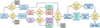 |
Fig. 1. Selection of dwarf galaxy samples from Apertif. The flowchart denotes most relevant steps in our selection procedure beginning from the Apertif source list to the dwarf galaxy samples used in this work. Boxes with bold text denote final samples used in our analysis. |
3.1. Correction for merged and multiple detections
To identify merged detections, we made use of Zooniverse4, by constructing a private project with all 2795 dwarf candidate sources in our initial sample. We used optical images from the PanSTARRS-1 photometric survey, infrared images from WISE, and ultraviolet images from GALEX, all overlaid with H I contours to visually classify each detection as corresponding to one or multiple galaxies. In some cases, we additionally inspected SIP outputs for Apertif H I detections to confirm our classification. With this, we identified 82 merged detections. For a subset of 11, the H I is poorly resolved, has low S/N, or both, making it unclear whether there are indeed multiple optical galaxies associated with the H I or if it is a happenstance alignment of multiple optical galaxies at different distances. For two of these cases, the multiple was confirmed by optical redshifts of candidate galaxies obtained from the NASA/IPAC Extragalactic Database5 (NED), while for the other nine cases there were no optical redshift measurements available for the confirmation. These nine cases are classified as “unclear” merged detections; see Appendix A for more information on these cases. In the rest of the paper, we treat them as merged detections, noting that the results do not change significantly by excluding these sources from the sample. For each merged detection, we used the same methodology described in Sect. 2.5 to measure stellar properties of companion galaxies. As for detections of single sources, we adopted individual galaxies in our sample only if their stellar properties could be reliably measured (e.g., no strong contamination by foreground stars). We applied this criterion independently on the companion and the original (previously measured) galaxy.
We searched for multiple detections of the same source based on the coordinates of the photometric measurements. We visually inspected all detections that have photometric measurements closer than 35″ on the sky. This relatively large radius was chosen because differences in the H I detections (especially split detections that can be spatially offset on the sky) could lead to the selection of different optical counterparts. Increasing this radius to 45″ (∼3 Apertif beams) did not provide any new multiple detection candidates. We then also checked for consistent recessional velocities between the duplicate detection candidates. In the end, 229 (out of 230) sources were confirmed to have been detected multiple times. For each multiple detection, we then chose one measurement of stellar and H I components of corresponding galaxies by visually inspecting H I total intensity maps and positions of available stellar measurements. For split detections, we summed the H I flux of the two detections in order to estimate the true H I mass of the galaxy.
After correcting for merged detections, multiple detections, and galaxies whose stellar measurement was compromised by a nearby star or a background galaxy (see Sect. 2.5), we end up with 2481 dwarf candidate galaxies, which we refer to as the parent dwarf galaxy sample (Fig. 1). The H I properties (systemic velocity and the H I mass) of galaxies in merged detections were measured by manually splitting the data cube (spatially) and extracting the spectrum of each galaxy individually. If galaxies in the merged detection were not spatially resolved in H I (25 merged detections, from which 48 galaxies entered the parent dwarf sample), we simply divided the total H I mass of the merged detection by the number of galaxies corresponding to that detection and assigned them the same Vsys corresponding to the merged detection.
3.2. Baryonic and dark matter halo masses
For each galaxy in our parent dwarf galaxy sample, we calculated its baryonic mass using:
 (2)
(2)
where a factor of 1.33 corrects for the contribution of helium to the gas mass of galaxies. We neglected the contribution of molecular gas in the calculation of Mb as molecular gas mass in low-mass galaxies has been shown to be significantly smaller than H I and stellar masses (around 10% of either) (see, e.g., Leroy et al. 2009; Bothwell et al. 2014; Accurso et al. 2017; Ponomareva et al. 2018; Catinella et al. 2018).
We assigned dark matter halo masses to galaxies in our parent sample using the stellar-to-halo mass relation (SHMR) from the semiempirical dwarf galaxy formation model DarkLight (Kim et al. 2024) applied to the dark-matter-only simulation of the void volume from the Engineering Dwarfs at Galaxy formation’s Edge (EDGE) project. The model is tailored to accurately predict dwarf galaxy properties down to the lowest masses by incorporating the relation between the SFR and dark matter halo properties pre- and post-reionization. Its application to the void volume provides us with a perfect relation for our H I selected (hence, naturally more isolated) sample of dwarf galaxies. The SHMR relation is
 (3)
(3)
where M200 is the virial mass of the dark matter halo, defined as the mass within R200, the radius within which the mean dark matter density is equal to 200 times the critical density of the Universe. We did not take into account the scatter of the relation as our goal is to trace the mass dependent effects in the selection of dwarf multiples (see Sect. 4), for which introducing the scatter would bring inconsistencies into our analysis (e.g., galaxies of the same stellar mass having different thresholds in projected separation and systemic velocity difference for companion assignment).
3.3. Properties of the parent dwarf galaxy sample
We show the distributions of stellar and H I masses of our parent dwarf sample in the left panel of Fig. 2. As mentioned at the beginning of the section, the sample includes galaxies with M⋆ measurement within 1σ level of our high mass limit of 5 × 10⁹ M⊙. Both distributions peak at masses around 109 M⊙ and steeply fall toward higher and lower masses. We are able to detect dwarfs down to stellar masses of 106 M⊙, but are biased toward high gas fraction as seen from the excess of stellar mass counts compared to the H I mass counts at the lower masses. This is a natural consequence of our H I-based selection. A similar excess of stellar mass counts (compared to the H I-mass ones) is seen also at the highest masses in our sample, which is a consequence of the anticorrelation of gas fraction and stellar mass of H I bearing galaxies (e.g., Huang et al. 2012). These trends in gas fraction are also seen in the right panel of Fig. 2 showing the systemic velocity (as a proxy for distance) dependence on the stellar mass of our sample. As expected, the lowest stellar mass galaxies are preferentially detected nearby and are more gas-rich. However, for stellar masses around 108 M⊙ and above, we are able to sample the whole available redshift range of our data. The robust quantification of completeness of our sample, however, is beyond the scope of this work.
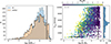 |
Fig. 2. Properties of the parent dwarf galaxy sample. Left: histograms of H I (blue) and stellar (orange) masses of the sample. The vertical line denotes the dwarf stellar mass limit of 5 × 10⁹ M⊙. Right: systemic velocity vs. stellar mass of dwarfs in the sample, color-coded by the gas fraction. We show typical stellar mass error in the upper left corner. The vertical line is the same as in the left plot. On the right, we plot the histogram along the Vsys axis of our sample. |
The histogram of Vsys is shown in the right panel of Fig. 2. While the distribution is uniform in the majority of our redshift range, there is a peak around systemic velocities of 5000 km s−1. This is a signature of the Perseus-Pisces filament within our footprint. In Sect. 4.2, we apply a strict isolation criterion to create a subsample of isolated galaxies, in which the overdensity at 5000 km s−1 completely disappears. We then present the properties (Sect. 4.2) and pair frequency (Sect. 5.1) of both our full sample and the highly isolated subsample.
4. Analysis
4.1. Selection of companions
To study the frequency of dwarf encounters, we aimed at finding dwarfs that are in close proximity to each other, i.e., that have one or more companions. We applied the following procedure to all realizations of our drawn dwarf galaxy sample (see below). A dwarf is assigned a companion if their projected distance (rp) and systemic velocity difference is less than a chosen threshold. We assigned companions to each galaxy individually, meaning that a lower mass dwarf can be assigned a companion of a higher mass (stellar and/or H I). Companions were assigned by a two-step approach, as described in the following.
In the first step, we used constant thresholds in rp and |ΔVsys| for all galaxies in the sample. As we aim to compare the abundance of close-by dwarfs found through our H I versus optical selection, we adopted the same criteria for the selection of pairs as in B18, corresponding to 150 kpc and 150 km s−1 in rp and |ΔVsys|, respectively. These thresholds were chosen by B18 to correspond to the virial radius and the escape velocity at that radius of the most massive galaxies in their mock catalog (M200 ∼ 4 × 10¹¹ M⊙) based on the hydrodynamical cosmological Illustris-1 simulation (Vogelsberger et al. 2014; Nelson et al. 2015). Hence, these thresholds served as an upper limit to the true physical thresholds for lower mass galaxies in the sample.
We applied these thresholds to each dwarf, treating all others in the sample as potential companions. The number of assigned companions varies for each dwarf and may differ from the count assigned to its companions, as illustrated in Fig. 3. An exception was made for dwarfs close to the spectral edges of Apertif cubes, that is, with Vsys < 424 + 150 = 574 km s−1 or Vsys > 10 170 − 150 = 10 020 km s−1; these were considered as companions to other dwarfs but were not assigned their own companions to avoid underestimating the number of companions due to cube limits. This constraint was not applied to spatial edges of Apertif fields, as fields within our spatial coverage are not necessarily contiguous, thereby leaving us with a complicated sky coverage. In addition, the sensitivity within our spatial footprint is generally highly nonuniform even within individual fields (see Sect. 2.1). A detailed assessment of these sensitivity variations is beyond the scope of this paper and will be addressed in a future study. For this work, not addressing these limitations can potentially only lead to a small suppression in the number of paired galaxies.
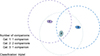 |
Fig. 3. Sketch of the classification of multiples. For simplicity, we show a case where all galaxies have the same stellar mass. The three galaxies are denoted with numbers one to three, and the selection criteria (both spatial and spectral) for companions are visualized as dashed (for galaxies 1 and 3) and dotted circles (for galaxy 2), centered at each galaxy. In this case, the number of companions is one for both galaxy 1 and 3, and two for galaxy 2. We classify this system as a triplet. |
In the second step, we aimed at making a more physical selection by scaling the thresholds in rp and |ΔVsys| with respect to the halo masses of the paired dwarfs found in the first step. We chose the new thresholds based on the dark matter halo masses obtained from the SHMR from the DarkLight model (Kim et al. 2024), and by applying the same physical definition as in the first step (virial radius and the escape velocity at that radius)6. We applied these thresholds by going through the list of galaxies who had one or more companions assigned in the first step and revisited the assignment of each companion again using the new scaled threshold. In each comparison between the reference galaxy and its initially assigned companion, the new scaled thresholds were calculated using the stellar mass of the more massive galaxy of the two.
Both these procedures were implemented on a series of 500 stochastic realizations of our dwarf galaxy sample, each derived by randomly drawing stellar masses assuming Gaussian error-bars in logarithmic space, and then filtering out galaxies with M⋆ < 5 × 10⁹ M⊙. Hence, for consistency, the halo mass used for the assignment of scaled thresholds was based on the drawn stellar mass of the galaxy in each realization. All the statistical quantities presented, along with their uncertainties, were determined using the mean values and the standard deviations between all 500 realizations. We refer to these realizations as the drawn dwarf galaxy sample (see Fig. 1), keeping in mind that the stellar mass of any one galaxy can change between realizations.
We report the number of pairs, triplets, and quadruplets found in our drawn dwarf galaxy sample in Table 1. Multiples (pairs, triplets, and quadruplets) were classified as sketched in Fig. 3, where galaxies were taken to be part of the same multiple if they are sharing a common companion. Taking the mass-scaled (constant) thresholds, the fraction of galaxies in a multiple of n galaxies (fn = n Nn/Ntot) is around 10% (12%) for pairs (n = 2, Nn = Npair), 2% (4%) for triplets (n = 3, Nn = Ntrip), and 0.1% (0.3%) for quadruplets (n = 4, Nn = Nquad).
Total number of multiples in the drawn dwarf galaxy sample
4.2. Isolation criteria
To ensure a consistent comparison with the previous optical study by B18, as well as to test the impact of the Perseus-Pisces filament on our results (see Sect. 3), we adopted the isolation criteria from B18, which ensure the dwarf galaxy is isolated from any massive galaxy (M⋆ > 5 × 10⁹ M⊙). The dwarf was not considered isolated if there was a massive galaxy satisfying both of the following criteria:
-
(a)
|ΔVsys|< 1000 km s−1, where |ΔVsys| is the absolute difference in systemic velocities between the massive galaxy and the dwarf;
-
(b)
tidal index Θ > −11.5, defined in Karachentsev et al. (2013) as:
![Mathematical equation: $$ \begin{aligned} \Theta = \log \left( \frac{M_{\star }^\mathrm{massive} [10^{11}\,M_\odot ]}{r_{\rm p}^3[\text{ Mpc}^3]} \right) - 10.97, \end{aligned} $$](/articles/aa/full_html/2025/11/aa54841-25/aa54841-25-eq6.gif) (4)
(4)where
 is the stellar mass of the massive galaxy, and rp is the projected separation between the massive galaxy and the dwarf.
Criteria a) is based on the findings of Patton et al. (2000) who showed that the |ΔVsys| distribution of galaxies in The Second Southern Sky Redshift Survey (da Costa et al. 1998) becomes indistinguishable from a random distribution at |ΔVsys|> 1000 km s−1. On the other hand, criteria b) is based on findings from Geha et al. (2012), which showed that the fraction of quenched dwarf galaxies drops to zero for projected distances greater than 1.5 Mpc from a luminous galaxy with K-band magnitudes below MK < −23 (corresponding to  ). This further corresponds to the tidal index of −11.5. Hence, these arguably stringent isolation criteria ensure dwarfs are well beyond the virial radius of any massive galaxy.
We applied the above criteria for each dwarf from the parent dwarf galaxy sample, which includes galaxies whose M⋆ measurement is compatible at the 1σ level with our higher mass limit of 5 × 10⁹ M⊙ (see Sect. 3). We first applied the above criteria, taking detections of massive galaxies (ones outside the parent dwarf sample) from the Apertif source list. This left us with 1244 candidate isolated dwarfs. We further proceeded to query NED within rp < 2 Mpc and |ΔVsys|< 1000 km s−1 around each of the remaining dwarfs, in order to find massive galaxies that might have been missed in Apertif (e.g., ones with low gas fractions) or that fall outside the Apertif footprint. During this process, we estimated stellar masses of NED galaxies using the W1 22.0″ radius aperture magnitude, and applying equation 2 from Wen et al. (2013). This left us with 735 isolated dwarf galaxy candidates (i.e., the parent isolated sample in Fig. 1). We note that by using a fixed aperture magnitude, we potentially underestimated stellar masses of high mass galaxies from NED (22″ corresponds to 7.5 kpc at our median distance of 70 Mpc). Taking the Milky Way (M⋆ = 5 × 10¹⁰ M⊙; e.g., Licquia & Newman 2016; McGaugh 2016) as an example, approximately 80% of its mass7 is enclosed within 7.5 kpc. This underestimates the projected separation required for isolation at 1.1 Mpc, instead of 1.2 Mpc. This small difference could result in the misclassification of a galaxy as isolated. It is, however, worth noting that most of the observed volume (V) is, and hence most of the massive galaxies are, beyond the median distance (V ∝ r3) where the effect is smaller. Furthermore, stellar distributions of gas-poor early-type galaxies are likely more concentrated than an exponential disk, making the effect milder than presented in the Milky Way example. Taking this into consideration together with the extreme strictness of the isolation criterion, we believe our approximate calculation of the stellar mass of high mass galaxies is sufficient to create a well-isolated dwarf galaxy sample. Finally, within each realization of the drawn dwarf galaxy sample, we further apply the isolation criteria for every dwarf with drawn M⋆ < 5 × 10⁹ M⊙, with regards to the ones whose drawn stellar mass exceeds this stellar mass limit. The final number of isolated dwarfs per realization is around ∼649 (i.e., the drawn isolated sample in Fig. 1).
In Fig. 4, we show the M⋆MH I relation and the M⋆–SFR relation of our isolated versus non-isolated galaxies in the parent dwarf sample. Generally, both relations show very good consistency between the two samples. The only systematic offset between the two populations is seen at the highest masses in the M⋆–MH I relation, with isolated galaxies being systematically more gas-rich. This is expected as higher-mass dwarfs can retain their gas content in closer proximity to high-mass galaxies, thereby remaining easily detectable in H I. However, we see no offset in the SFRs between the two populations, implying that the impact of the environment only influenced the non-starforming gas reservoir (e.g., at the galaxies’ outskirts, by gas stripping). The apparent larger H I masses for non-isolated dwarfs at very low masses is not statistically significant due to the low number of objects (≤8 per bin in either sample). Hence, while there are signatures of environmental impacts on the highest mass galaxies in our parent dwarf sample, it is unlikely that we have strong contamination from dwarfs in direct close-by interactions with a high-mass galaxy, meaning that our total sample is still mostly dominated by reasonably well-isolated dwarfs.
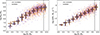 |
Fig. 4. Comparison of galaxy properties between the isolated and non-isolated subsamples of our parent dwarf sample. Left: M⋆–MH I relation. Isolated galaxies are plotted as purple squares, and non-isolated as orange circles. The error bars represent the median values and percentile errors, with the isolated sample shown as full purple lines, and non-isolated as dashed orange lines. The vertical black line denotes the stellar mass limit of 5 × 10⁹ M⊙. Right: M⋆–SFR relation. The markings are the same as in the left panel. |
Interestingly, the number of multiples found in the isolated drawn galaxy sample does not deviate significantly from the number of multiples in our total drawn sample, as seen from Table 1. The absolute fractional difference in the number of galaxies in multiples (|fntotal − fnisolated|) for mass-scaled (constant) thresholds are 1.1% (1.3%) for pairs, 0.7% (0.8%) for triplets, and 0.1% (0.2%) for quadruplets.
5. Results
5.1. Frequency of dwarf galaxy multiples
In this section, we investigate how the average number of dwarf galaxy companions depends on the stellar mass of the dwarf, or in other words, how many companions a dwarf of a specific stellar mass is expected to have on average. We show our results in terms of the mean number of companions per galaxy per stellar mass bin (Nc, m; Patton et al. 2000, B18), calculated by summing the number of companions (of any stellar mass) of all dwarfs corresponding to the stellar mass bin, and by dividing by the total number of dwarfs in that mass bin.
In Fig. 5, we compare our results obtained by applying constant thresholds for projected distance and systemic velocity difference for the selection of companions (from the first step in our analysis, see Sect. 4.1), and the ones obtained after applying the mass-scaled thresholds on our total drawn dwarf galaxy sample (without applied isolation). In both cases the mean number of companions rises as we go down toward lower stellar masses, with the rise being significantly milder with the use of the mass-scaled thresholds. This difference corresponds to potential non-physical associations present when using constant thresholds (scaled to the highest stellar masses in the sample) for companion selection of lower mass dwarfs. This trend is also found in simulations, for example, Huško et al. (2022) and Chamberlain et al. (2024). Hence, using mass-scaled thresholds is necessary to systematically constrain the fractions of dwarf companions in Apertif, and we use them in the rest of the paper, unless stated otherwise.
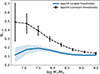 |
Fig. 5. Mean number of companions (of any stellar mass) per dwarf galaxy in the logarithmic stellar mass bin, normalized by the number of dwarfs in the same mass bin. Values represent the mean between different realizations of the sample in each mass bin. The black line represents results obtained using constant thresholds in projected distance and systemic velocity difference (150 kpc and 150 km s−1, respectively) for selection of companions, while the blue line represents results obtained using the mass-scaled thresholds (see Sect. 4.1). Both lines represent results for the total drawn dwarf galaxy sample. Shaded regions and error bars represent 1σ errors. |
In the mass-scaled case, the slight increase in the mean number of companions toward lower stellar masses is still expected due to our stellar mass cut on the sample. At the highest masses in our sample, we are, for example, only counting half of the major pairs these galaxies are a part of, the ones in which they are preferentially the hosts (most massive in the pair / multiple). Similarly, at the lowest masses, we are only counting pairs in which the reference galaxy is a satellite (not the most massive in the multiple), contributing to the slight turndown in the number of companions. Finally, for dwarfs in the middle of our mass range, we are counting both cases, when they are either the host or the satellite. Despite these expectations, this trend is mild in our sample, as the mean number of companions with scaled thresholds is consistent with a constant value within 2σ. The exact shape of the trend, however, inherently depends on the slope of the adopted SHMR (Eq. (3)), which is used to define the mass-scaled thresholds. Shallower SHMRs would give a slightly stronger increase in the mean number of companions toward lower stellar masses. In summary, by adopting the DarkLight SHMR, we find that the mean number of companions per dwarf (taking the whole mass range) is (12.8 ± 0.4)% in our sample.
The comparison of results for our total drawn sample and our isolated drawn sample is shown in Fig. 6, where we show binnings both in stellar and baryonic masses. In this plot, we use the median and the percentile errors in each stellar (left panel) and baryonic (right panel) mass bin due to low number statistics in the lowest mass bins. We plot two cases for the isolated sample because some multiples (∼10, depending on the realization) would be split after applying the criteria (i.e., one galaxy passed the isolation criteria while the other has not). Given that the multiples are chosen to be close-by and our isolation criteria are strict, we prefer to either include or exclude the whole multiple when counting. Hence, we show a case with all galaxies within a split multiple corresponding to our upper limit (purple) and a case with none of the galaxies in a split multiple corresponding to our lower limit (pink). The mean number of companions in both cases is fully consistent with the result from the total drawn sample, but seems to show a steeper increase toward lower stellar (and baryonic) masses at higher mass bins (even though still consistent with a constant distribution at 2σ). This might indicate an influence of the large-scale structure on the groupings of dwarf galaxies. However, the general consistency of the isolated and full sample shows us that the impact (if real) on our sample is minor, which is consistent with our H I-based selection that is already biased toward isolated galaxies.
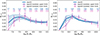 |
Fig. 6. Mean number of companions (of any stellar and/or baryonic mass) per dwarf in logarithmic stellar (left) or baryonic (right) mass bins, normalized by the number of dwarfs per bin. Values represent the median between different realizations of the sample in each mass bin. All lines are obtained using mass-scaled thresholds (see Sect. 4.1): the blue line represents the total drawn dwarf galaxy sample, the dashed purple line the isolated drawn sample including split multiples (upper limit), and the dotted pink line the isolated drawn sample excluding split multiples (lower limit). Shaded regions and error bars indicate 1σ uncertainties. The number of galaxies in each bin is shown at the top, with font colors and order matching the corresponding lines in the legend. |
5.2. Star formation rate of paired galaxies
As shown in previous studies (e.g., Kado-Fong et al. 2024; Huang et al. 2025), close galaxy encounters can enhance and suppress star formation in dwarf galaxies. Different mechanisms have been proposed for the SFR enhancement in gas-rich high- and low-mass galaxies (Huang et al. 2025). To explore if such trends are present in our sample, we selected pairs of dwarfs identified in at least one realization of our total drawn galaxy sample using constant thresholds (from the first step of our analysis, see Sect. 4.1). We used these looser thresholds to obtain better statistics, noting that they are relatively strict compared to previously used ones in similar studies (e.g., 250 kpc and 500 km s−1 used in Huang et al. 2025). The total number of pairs obtained is 147. We considered only galaxies in pairs and not higher multiples for easier interpretation. In this section, we use the original stellar mass measurement (corresponding to the parent galaxy sample) instead of the drawn value.
For each galaxy in a pair, we assigned a control sample of five or more unpaired dwarfs (ones with no companion in any realization) that have both stellar and H I masses within 0.1 dex of the paired dwarfs. In the 47 cases for which fewer than five single dwarfs satisfied the criteria, we excluded the paired dwarf from the analysis. Following the approach of Huang et al. (2025), we defined the SFR offset (Δlog SFR) as the difference between the SFR of the paired dwarf and the median of the SFRs of its control sample. The error on this median was obtained by bootstrapping SFRs of the control sample. Furthermore, to estimate the significance of any possible offsets, we randomly selected around 250 unpaired galaxies and repeated the above procedure in which we assigned them their own control sample and calculate their Δlog SFR. We then used the 1σ and 2σ scatter of the unpaired dwarfs for our comparison to paired dwarfs.
Fig. 7 shows the Δlog SFR with respect to the projected distance of individual galaxies in pairs, scaled by the virial radius of the pair. As in Huang et al. (2025), this virial radius is calculated using the halo mass of the pair, which we estimated by summing the halo masses (see Sect. 3.2) of individual galaxies. We distinguished the primary and secondary galaxies as the more and less massive (in stellar mass) members of the pair, respectively, and separated our sample into high and low stellar mass ratio ( ) pairs based on the threshold of 1/3. In the low (SMR < 1/3) SMR case, we calculated running means for primary and secondary galaxies separately, while for the high (SMR > 1/3) SMR case we did not make this distinction as galaxies within a pair are comparable in mass. We calculated the running means in the SMR > 1/3 case using the kernel size of 10, corresponding to the mean span in
  (in the running mean calculation) of 0.07 for scaled separations below 0.3, 0.19 between 0.3 and 0.6, and 0.13 between 0.6 and 0.9. To roughly match the same mean rp/
 span and similar statistical significance in the SMR < 1/3 case, we used the kernel size of 8, corresponding to the mean span of 0.16 and 0.20 for primaries and secondaries, respectively. Errors on the running mean were obtained by bootstrapping the Δlog SFR offsets of paired galaxies and taking the mean and the standard deviation of the running mean between 104 realizations.
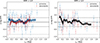 |
Fig. 7. Difference in the SFRs of paired galaxies with respect to the unpaired control sample vs. the pair separation scaled by the virial radius of the pair. Left: pairs with stellar mass ratios below 1/3. Primaries correspond to the more massive galaxy in a pair and are denoted by blue squares, while secondaries (the less massive in a pair) are denoted by red circles. Blue and red lines correspond to the running means for primaries and secondaries, respectively, with 1σ errors on the means denoted as shaded regions. Horizontal dashed and dotted black lines denote the 1σ and 2σ scatter of unpaired galaxies. Right: pairs with stellar mass ratios above 1/3. The notation is the same as in the left panel, except that the running mean (black line) is calculated by taking primary and secondary galaxies together. |
In both high and low SMR cases, the scatter of paired galaxies (both primaries and secondaries) is comparable to the scatter of unpaired dwarfs at all scaled separations. However, for high SMRs and at scaled separations below 0.2, a few paired dwarfs exhibit SFR enhancements above the 2σ scatter of unpaired galaxies, up to around 1 dex compared to their unpaired control samples. There is also a systematic increase in the running mean at these separations, reaching 0.33 dex above the mean of the unpaired dwarfs (zero enhancement). At larger separations, the density of the points decreases, so the observed trend is less well constrained. It is, however, clear that we do not see any significant SFR suppression at any scaled separation in this case.
For low SMRs, we see no significant trend between primary and secondary galaxies with respect to the scaled separation, but there is a hint of the SFR enhancement of primaries and SFR suppression of secondaries at the lowest separations (below 0.2). However, primaries do seem to show a systematic SFR enhancement at almost all separations (∼0.09 dex, on average).
6. Discussion
6.1. Frequency of pairs in optical versus our H I sample
We compare the mean number of companions in our sample to results from B18, who studied the number of dwarf multiples found in SDSS spectroscopic data within a stellar mass range of 2 × 10⁸ < M⋆/M⊙ < 5 × 10⁹. They used constant thresholds in their selection of companions, exactly corresponding to the first step in our selection (Sect. 4.1), and applied the same isolation criteria that we employ in our sample (Sect. 4.2). They imposed an additional criterion in their selection of companions, namely that the projected radius between pairs is rp > 55″ to avoid incompleteness due to fiber collisions. In the following comparison, we cut our drawn dwarf galaxy samples to the same stellar mass range to ensure a consistent comparison and explore cases with and without applying the additional criterion on rp.
The comparison between B18 and our results can be seen in Fig. 8, where in the left panel we do not apply the additional criterion on the projected radius (rp > 55″), and in the right panel we do. For each of these cases, we show results with and without applying the isolation criteria to our sample (Sect. 4.2). We include the latter case in the comparison with B18 as our full sample contains a comparative number of galaxies in the sample as in B18 (∼1660 in our Apertif sample, and ∼1910 in SDSS) and is likely still dominated by field galaxies (see Sect. 4.2), thereby making for a more statistically consistent comparison. For the case with applied isolation, we take the lower limit where we exclude pairs even if only one dwarf did not pass the isolation criteria (see Sect. 5.1).
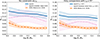 |
Fig. 8. Comparison of the mean number of companions per dwarf between the Apertif and the SDSS samples. Left: case with no constraint on the projected radius between companions in Apertif. The blue line represents the result for the total drawn galaxy sample; the dotted pink represents the results from the isolated drawn sample by taking the lower limit (see Sect. 5.1); and the dashed orange line represents results from B18. Shaded regions represent 1σ errors. Right: same as in the left panel, but excluding all companions in Apertif for which rp < 55″. |
Overall, in all these comparisons, our Apertif (H I selected) sample returns a higher mean number of companions per dwarf galaxy. In the case without applying the additional selection criteria (left panel), the full Apertif sample is remarkably higher in all mass bins. This remains true even when the isolation criteria is applied to the sample, although the reduced number of galaxies in the Apertif sample (∼443 galaxies) means it becomes consistent within 2σ. When considering the additional criteria to avoid close companions (rp > 55″; right panel) and applying the same isolation criteria, the two samples become formally consistent, although our values are still systematically higher across most of the mass range. However, this is limited by the small number of galaxies remaining in the Apertif sample leading to large uncertainties. In comparison, when taking our full sample, the mean number of companions is (11.6 ± 0.5)%, consistently higher than in B18, and also remains higher than their predicted value of 6% for a stellar mass complete survey.
A possible explanation for the offset between our H I selected sample and the B18 sample could be the additional galaxy population we are probing. Optical spectroscopic studies are biased against detecting low-surface-brightness galaxies, while in H I we are able to easily detect all gas-rich dwarfs independently of their stellar content and obtain the redshift information at the same time. Hence, cases in which the interaction disturbs the morphology of an interacting dwarf (potentially lowering its surface brightness) might be missed in optical surveys, thereby leading to a lower fraction of multiples.
Our result suggests that H I surveys are able to find three times higher percentage of multiples than optical surveys. Further studies with larger samples are needed to robustly constrain how different selections impact the retrieved number of multiples and how significant the offset we are finding truly is. It is, however, clear that H I surveys allow the identification of closer pairs by not suffering from fiber collisions and thus provide a crucial window for quantifying the actual number of dwarf galaxy multiples in the field as well as studying the closest part of their interactions. These results can be directly compared to the clustering of galaxies in the low mass regime of current state-of-the-art simulations, thereby constraining the structure formation in current models, the implementation of sub-grid physics (especially during dwarf-dwarf interactions), and, hence, galaxy evolution at small scales. Finally, as H I surveys are naturally unbiased by the stellar content, the impact that the interaction has on the dwarf (e.g., lowering the surface brightness due to tidal effects or enhancing the surface brightness by enhancing the SFR) will not impact the selection of the dwarf, making the estimate of pair fractions more robust than in the optical.
6.2. Properties of H I selected dwarf pairs
A recent work by Huang et al. (2025) studied how close encounters of gas-rich galaxies influence their SFRs. They selected galaxy pairs from the WALLABY H I survey, using thresholds in projected radius and velocity difference of 250 kpc and 500 km s−1, respectively. They also excluded higher-order multiples by requiring that neither galaxy in a pair has another companion within 250 kpc and 500 km s−1, and ensured that none of the pairs are located within known galaxy groups to guarantee isolation. Their sample spans the stellar mass range of 107.6–1011.2 M⊙. For each paired galaxy, they have made a control sample by matching in stellar and H I masses, and redshift, from a control pool of galaxies that have no imposed constraints (including no isolation constraint).
They separated their sample into low- and high-mass galaxies based on the stellar mass limit of 109 M⊙ but allow their low-mass galaxies to be paired with high-mass ones. For their low-mass galaxy sample, the SFRs initially decrease below  with maximum SFR suppression of ∼0.22 dex (at 1.4σ significance) at scaled separations of 0.6. Only at separations
  , they find a steep SFR enhancement of magnitude ∼0.22 dex. As seen in Sect. 5.2, the high SMR pairs in our sample show the SFR enhancement at separations
  , but no clear indication of systematic SFR suppression. This holds true even if we apply the upper stellar mass limit of 109 M⊙, as in Huang et al. (2025). However, in the low SMR pairs we do find a tentative SFR suppression for secondaries at separations below 0.2, indicating that the large difference in mass might be needed in order to suppress the star formation in the lower mass galaxy. We note that, differently from Huang et al. (2025), we do not include dwarf-high mass galaxy interactions in our analysis. Hence, such interactions can potentially have a much stronger influence on the star-formation activity of dwarf galaxies in their work, thereby inducing stronger and potentially traceable trends.
6.3. Impact of merged detections
As described in Sect. 3.1, the parent dwarf galaxy sample contains dwarf galaxies that were detected as part of a merged H I detection (155 out of 2481 galaxies in the sample). It is possible that some merged detections include emission from dwarf galaxies that would have been missed as an independent H I detection due to being individually too faint (i.e., close to or below the detection limit). If true, this would possibly bias our results toward a higher mean number of companions per dwarf.
As a first estimate of the impact of potential biases merged detections could have on our sample, we plot the distribution of H I fluxes of galaxies in our parent dwarf sample in Fig. 9, distinguishing between those detected individually and those found in merged detections. If there were no biases in our sample, we would expect these two distributions to have the same shape. While the distributions are indeed similar in shape, there seems to be a small tail toward lower fluxes for the case of merged detections. This indicates that some galaxies in our sample would possibly not be detected as an individual source. To estimate the impact of this on our results, we exclude all galaxies (corresponding to either single or merged detections) in the lowest five flux bins and rerun our analysis. The result is shown as a dotted gray line in Fig. 10. The result is completely consistent with our original run, with only a 1% offset (on average) toward a lower mean number of companions.
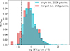 |
Fig. 9. Flux distributions for galaxies found in merged detections (red) vs. separate detections (cyan) in our parent dwarf galaxy sample. Histograms are normalized to the number of galaxies in each sample (reported in the legend). The vertical dashed black line denotes the flux limit of 0.187 Jy km s−1 below which there is an excess of galaxies detected in merged detections. |
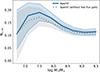 |
Fig. 10. Mean number of companions (of any stellar mass) per dwarf in the logarithmic stellar mass bin, normalized by the number of dwarfs in the same mass bin. Values represent the median between different realizations of the sample in each mass bin. The blue line represents results for the total drawn dwarf galaxy sample, and the dotted gray line represents the results obtained by excluding all sources below the 0.187 Jy km s−1 threshold in the H I flux. Shaded regions represent 1σ errors. |
Hence, the true number of companions is most likely close to our original result. The robust quantification of any potential biases in our sample (e.g., by repeating the source finding procedure with mock sources) is, however, beyond the scope of this work.
7. Conclusions
In this work, we presented for the first time the frequency of dwarf galaxy multiples found in an interferometric, untargeted H I survey. Our parent dwarf galaxy sample is based on detections from the Apertif H I survey and spans the stellar mass range between ∼106 M⊙ and ∼5 × 10⁹ M⊙ (including higher mass galaxies within 1σ of this threshold), containing 2481 candidate dwarf galaxies. We searched for paired galaxies by imposing thresholds in the projected radius and the difference in systemic velocity using two approaches. Firstly, we applied the constant thresholds corresponding to rp < 150 kpc and |ΔVsys|< 150 km s−1 for all galaxies independently of their stellar mass, in analogy to the previous work based on optical spectroscopy by B18. In the second step, we applied mass-scaled thresholds based on the SHMR from Kim et al. (2024) and corresponding to the virial radius and the escape velocity at that radius. We applied a strict isolation criterion to our sample to ensure consistent comparison with previous studies. Finally, we studied the SFR enhancement in pairs identified in our first step (using constant thresholds) with respect to the projected separation of the pair scaled by its virial radius. We summarize our findings in the following:
-
We find that the mean number of companions per dwarf is ∼12.8% in our H I selected dwarfs sample (Fig. 5). This is the first quantification of the fraction of dwarf galaxy multiples in an untargeted H I survey.
-
We do not find large differences between the total H I-detected dwarf galaxy sample and a highly isolated subsample in either global galaxy properties or the mean number of companions per dwarf (Figs. 4 and 6). This indicates that an H I-selected dwarf galaxy sample is already well isolated, in line with previous studies from the literature.
-
We are able to detect a fraction of dwarf galaxy pairs in the Apertif H I survey that is three times higher than that found in the SDSS optical spectroscopic survey (Fig. 8). This illustrates the power of H I for finding dwarf pairs, especially close pairs where fiber collisions are a strong limitation for existing optical spectroscopic surveys.
-
Pairs of galaxies with comparable stellar masses (stellar mass ratios between 1/3 - 1) in Apertif show SFR enhancement at projected separations ≲0.2
 on the order of ∼0.33 dex. We also find a hint of SFR suppression of less massive galaxies in pairs with larger mass difference (stellar mass ratios below 1/3), indicating that a significant difference in mass is needed for the suppression of the SFR in dwarf galaxies.
This study exemplifies the power of untargeted, interferometric H I surveys in robustly constraining the true frequency of dwarf galaxy multiples in observations. The frequency of galaxy encounters, together with studying the influence of such encounters on galaxy properties, is crucial for disentangling a galaxy’s secular evolution from its environment. Hence, our results could serve as a direct test of galaxy evolution models by comparison with current state-of-the-art simulations, both in the frequency of dwarf multiples and the properties of interacting galaxies.
Data availability
The parent dwarf galaxy sample used in this work is available at the CDS via https://cdsarc.cds.unistra.fr/viz-bin/cat/J/A+A/703/A295
This corresponds to 144 kpc and 153 km s−1 for stellar masses of 5 × 10⁹ M⊙ when taking the SHMR from DarkLight. The 3 km s−1 increase in the spectral threshold, compared to the initial constant thresholds, is smaller than half the channel width of Apertif and hence would not make a significant difference in our results.
Assuming an exponential stellar disk with the scale length of 2.5 kpc.
Acknowledgments
We thank the anonymous referee for valuable comments that improved this manuscript. KMH, JG, and SSE acknowledge financial support from the grant CEX2021-001131-S funded by MCIN/AEI/ 10.13039/501100011033 from the coordination of the participation in SKA-SPAIN funded by the Ministry of Science and Innovation (MCIN); and from grant PID2021-123930OB-C21 funded by MCIN/AEI/ 10.13039/501100011033 by “ERDF A way of making Europe” and by the “European Union”. Authors KMH, BŠ, JG, SSE acknowledge the Spanish Prototype of an SRC (SPSRC) service and support funded by the Ministerio de Ciencia, Innovación y Universidades (MICIU), by the Junta de Andalucía, by the European Regional Development Funds (ERDF) and by the European Union NextGenerationEU/PRTR. The SPSRC acknowledges financial support from the Agencia Estatal de Investigación (AEI) through the “Center of Excellence Severo Ochoa” award to the Instituto de Astrofísica de Andalucía (IAA-CSIC) (SEV-2017-0709) and from the grant CEX2021-001131-S funded by MICIU/AEI/ 10.13039/501100011033. KMH and JMvdH acknowledge funding from the ERC under the European Union’s Seventh Framework Programme (FP/2007–2013)/ERC Grant Agreement No. 291531 (‘HIStoryNU’). This work has received funding from the European Research Council (ERC) under the Horizon Europe research and innovation programme (Acronym: FLOWS, Grant number: 101096087). This work makes use of data from the Apertif system installed at the Westerbork Synthesis Radio Telescope owned by ASTRON. ASTRON, the Netherlands Institute for Radio Astronomy, is an institute of the Dutch Research Council (“De Nederlandse Organisatie voor Wetenschappelijk Onderzoek”, NWO). This publication uses data generated via the Zooniverse.org platform, development of which is funded by generous support, including a Global Impact Award from Google, and by a grant from the Alfred P. Sloan Foundation. This work made use of Astropy: (http://www.astropy.org) a community-developed core Python package and an ecosystem of tools and resources for astronomy (Astropy Collaboration 2013, 2018, 2022). This research has made use of the NASA/IPAC Extragalactic Database (NED), which is operated by the Jet Propulsion Laboratory, California Institute of Technology, under contract with the National Aeronautics and Space Administration. This publication makes use of data products from the Wide-field Infrared Survey Explorer, which is a joint project of the University of California, Los Angeles, and the Jet Propulsion Laboratory/California Institute of Technology, funded by the National Aeronautics and Space Administration. This work is based in part on observations made with the Spitzer Space Telescope, which was operated by the Jet Propulsion Laboratory, California Institute of Technology under a contract with NASA. GALEX is a NASA Small Explorer, launched in 2003 April, operated for NASA by the California Institute of Technology under NASA contract NAS5-98034. The Pan-STARRS1 Surveys (PS1) have been made possible through contributions of the Institute for Astronomy, the University of Hawaii, the Pan-STARRS Project Office, the Max-Planck Society and its participating institutes, the Max Planck Institute for Astronomy, Heidelberg and the Max Planck Institute for Extraterrestrial Physics, Garching, The Johns Hopkins University, Durham University, the University of Edinburgh, Queen’s University Belfast, the Harvard-Smithsonian Center for Astrophysics, the Las Cumbres Observatory Global Telescope Network Incorporated, the National Central University of Taiwan, the Space Telescope Science Institute, the National Aeronautics and Space Administration under Grant No. NNX08AR22G issued through the Planetary Science Division of the NASA Science Mission Directorate, the National Science Foundation under Grant No. AST-1238877, the University of Maryland, and Eotvos Lorand University (ELTE). The flowchart in this paper was created using the Miro online collaborative whiteboard platform (www.miro.com).
References
- Accurso, G., Saintonge, A., Catinella, B., et al. 2017, MNRAS, 470, 4750 [NASA ADS] [Google Scholar]
- Adams, E. A. K., Adebahr, B., de Blok, W. J. G., et al. 2022, A&A, 667, A38 [NASA ADS] [CrossRef] [EDP Sciences] [Google Scholar]
- Adebahr, B., Schulz, R., Dijkema, T. J., et al. 2022, Astron. Comput., 38, 100514 [NASA ADS] [CrossRef] [Google Scholar]
- Astropy Collaboration (Robitaille, T. P., et al.) 2013, A&A, 558, A33 [NASA ADS] [CrossRef] [EDP Sciences] [Google Scholar]
- Astropy Collaboration (Price-Whelan, A. M., et al.) 2018, AJ, 156, 123 [Google Scholar]
- Astropy Collaboration (Price-Whelan, A. M., et al.) 2022, ApJ, 935, 167 [NASA ADS] [CrossRef] [Google Scholar]
- Barnes, J. E., & Hernquist, L. 1992, ARA&A, 30, 705 [Google Scholar]
- Bennet, P., Sand, D. J., Zaritsky, D., et al. 2018, ApJ, 866, L11 [NASA ADS] [CrossRef] [Google Scholar]
- Bertin, E., & Arnouts, S. 1996, A&AS, 117, 393 [NASA ADS] [CrossRef] [EDP Sciences] [Google Scholar]
- Besla, G., Patton, D. R., Stierwalt, S., et al. 2018, MNRAS, 480, 3376 [NASA ADS] [CrossRef] [Google Scholar]
- Blanton, M. R., Lupton, R. H., Schlegel, D. J., et al. 2005, ApJ, 631, 208 [Google Scholar]
- Bothwell, M. S., Wagg, J., Cicone, C., et al. 2014, MNRAS, 445, 2599 [NASA ADS] [CrossRef] [Google Scholar]
- Cannon, J. M., Martinkus, C. P., Leisman, L., et al. 2015, AJ, 149, 72 [NASA ADS] [CrossRef] [Google Scholar]
- Catinella, B., Saintonge, A., Janowiecki, S., et al. 2018, MNRAS, 476, 875 [NASA ADS] [CrossRef] [Google Scholar]
- Chamberlain, K., Besla, G., Patel, E., et al. 2024, ApJ, 962, 162 [NASA ADS] [CrossRef] [Google Scholar]
- Chambers, K. C., Magnier, E. A., Metcalfe, N., et al. 2016, ArXiv e-prints [arXiv:1612.05560] [Google Scholar]
- da Costa, L. N., Willmer, C. N. A., Pellegrini, P. S., et al. 1998, AJ, 116, 1 [Google Scholar]
- Dillamore, A. M., Belokurov, V., Font, A. S., & McCarthy, I. G. 2022, MNRAS, 513, 1867 [NASA ADS] [CrossRef] [Google Scholar]
- Duncan, K., Conselice, C. J., Mundy, C., et al. 2019, ApJ, 876, 110 [NASA ADS] [CrossRef] [Google Scholar]
- Ellison, S. L., Patton, D. R., Simard, L., & McConnachie, A. W. 2008, AJ, 135, 1877 [NASA ADS] [CrossRef] [Google Scholar]
- Eróstegui, A., Mezcua, M., Siudek, M., Domínguez Sánchez, H., & Rodríguez Morales, V. 2025, A&A, 699, A330 [NASA ADS] [CrossRef] [EDP Sciences] [Google Scholar]
- Fasano, G., Vanzella, E., Dressler, A., et al. 2012, MNRAS, 420, 926 [Google Scholar]
- Vallenari, A. 2023, A&A, 674, A1 [Google Scholar]
- Gao, F., Wang, L., Pearson, W. J., et al. 2020, A&A, 637, A94 [NASA ADS] [CrossRef] [EDP Sciences] [Google Scholar]
- Geha, M., Blanton, M. R., Masjedi, M., & West, A. A. 2006, ApJ, 653, 240 [NASA ADS] [CrossRef] [Google Scholar]
- Geha, M., Blanton, M. R., Yan, R., & Tinker, J. L. 2012, ApJ, 757, 85 [Google Scholar]
- Giovanelli, R., Haynes, M. P., Kent, B. R., et al. 2005, AJ, 130, 2598 [Google Scholar]
- Goulding, A. D., Greene, J. E., Bezanson, R., et al. 2018, PASJ, 70, S37 [NASA ADS] [CrossRef] [Google Scholar]
- Haubner, K., Lelli, F., Di Teodoro, E., et al. 2025, A&A, 696, A185 [NASA ADS] [CrossRef] [EDP Sciences] [Google Scholar]
- Haynes, M. P., Giovanelli, R., Kent, B. R., et al. 2018, ApJ, 861, 49 [Google Scholar]
- Hess, K. M., Paoloserra, Boschman, L., Shen, A., & Julia, H. 2024, https://doi.org/10.5281/zenodo.14016958 [Google Scholar]
- Holincheck, A. J., Wallin, J. F., Borne, K., et al. 2016, MNRAS, 459, 720 [NASA ADS] [CrossRef] [Google Scholar]
- Huang, Q., Wang, J., Lin, X., et al. 2025, ApJ, 980, 157 [Google Scholar]
- Huang, S., Haynes, M. P., Giovanelli, R., & Brinchmann, J. 2012, ApJ, 756, 113 [Google Scholar]
- Huško, F., Lacey, C. G., & Baugh, C. M. 2022, MNRAS, 509, 5918 [Google Scholar]
- Janowiecki, S., Leisman, L., Józsa, G., et al. 2015, ApJ, 801, 96 [NASA ADS] [CrossRef] [Google Scholar]
- Jarvis, M. J., Taylor, A. R., Agudo, I., et al. 2017, The MeerKAT International GHz Tiered Extragalactic Exploration (MIGHTEE) Survey [Google Scholar]
- Kado-Fong, E., Robinson, A., Nyland, K., et al. 2024, ApJ, 963, 37 [NASA ADS] [CrossRef] [Google Scholar]
- Karachentsev, I. D., Makarov, D. I., & Kaisina, E. I. 2013, AJ, 145, 101 [Google Scholar]
- Kartaltepe, J. S., Sanders, D. B., Scoville, N. Z., et al. 2007, ApJS, 172, 320 [NASA ADS] [CrossRef] [Google Scholar]
- Kennicutt, R. C., & Evans, N. J. 2012, ARA&A, 50, 531 [NASA ADS] [CrossRef] [Google Scholar]
- Kim, S. Y., Read, J. I., Rey, M. P., et al. 2024, ArXiv e-prints [arXiv:2408.15214] [Google Scholar]
- Koribalski, B. S., Staveley-Smith, L., Westmeier, T., et al. 2020, Ap&SS, 365, 118 [Google Scholar]
- Kourkchi, E., Courtois, H. M., Graziani, R., et al. 2020, AJ, 159, 67 [NASA ADS] [CrossRef] [Google Scholar]
- Kumar, A., Das, M., & Kataria, S. K. 2021, MNRAS, 506, 98 [NASA ADS] [CrossRef] [Google Scholar]
- Kutkin, A. M., Oosterloo, T. A., Morganti, R., et al. 2022, A&A, 667, A39 [NASA ADS] [CrossRef] [EDP Sciences] [Google Scholar]
- La Marca, A., Margalef-Bentabol, B., Wang, L., et al. 2024, A&A, 690, A326 [NASA ADS] [CrossRef] [EDP Sciences] [Google Scholar]
- Leisman, L., Haynes, M. P., Janowiecki, S., et al. 2017, ApJ, 842, 133 [NASA ADS] [CrossRef] [Google Scholar]
- Leroy, A. K., Walter, F., Bigiel, F., et al. 2009, AJ, 137, 4670 [Google Scholar]
- Leroy, A. K., Sandstrom, K. M., Lang, D., et al. 2019, ApJS, 244, 24 [Google Scholar]
- Li, C., Kauffmann, G., Heckman, T. M., Jing, Y. P., & White, S. D. M. 2008, MNRAS, 385, 1903 [NASA ADS] [CrossRef] [Google Scholar]
- Licquia, T. C., & Newman, J. A. 2016, ApJ, 831, 71 [CrossRef] [Google Scholar]
- Marasco, A., Belfiore, F., Cresci, G., et al. 2023, A&A, 670, A92 [NASA ADS] [CrossRef] [EDP Sciences] [Google Scholar]
- Marasco, A., Fall, S. M., Di Teodoro, E. M., & Mancera Piña, P. E. 2025, A&A, 695, L23 [NASA ADS] [CrossRef] [EDP Sciences] [Google Scholar]
- Martin, D. C., Fanson, J., Schiminovich, D., et al. 2005, ApJ, 619, L1 [Google Scholar]
- Martin, G., Kaviraj, S., Devriendt, J. E. G., Dubois, Y., & Pichon, C. 2018, MNRAS, 480, 2266 [Google Scholar]
- Martin, G., Jackson, R. A., Kaviraj, S., et al. 2021, MNRAS, 500, 4937 [Google Scholar]
- McGaugh, S. S. 2016, ApJ, 816, 42 [Google Scholar]
- Meyer, M. J., Zwaan, M. A., Webster, R. L., et al. 2004, MNRAS, 350, 1195 [Google Scholar]
- Moore, B., Katz, N., Lake, G., Dressler, A., & Oemler, A. 1996, Nature, 379, 613 [Google Scholar]
- Nelson, D., Pillepich, A., Genel, S., et al. 2015, Astron. Comput., 13, 12 [Google Scholar]
- Patton, D. R., Carlberg, R. G., Marzke, R. O., et al. 2000, ApJ, 536, 153 [NASA ADS] [CrossRef] [Google Scholar]
- Ponomareva, A. A., Verheijen, M. A. W., Papastergis, E., Bosma, A., & Peletier, R. F. 2018, MNRAS, 474, 4366 [Google Scholar]
- Sales, L. V., Wang, W., White, S. D. M., & Navarro, J. F. 2013, MNRAS, 428, 573 [NASA ADS] [CrossRef] [Google Scholar]
- Salim, S., Lee, J. C., Janowiecki, S., et al. 2016, ApJS, 227, 2 [NASA ADS] [CrossRef] [Google Scholar]
- Salim, S., Boquien, M., & Lee, J. C. 2018, ApJ, 859, 11 [Google Scholar]
- Satyapal, S., Ellison, S. L., McAlpine, W., et al. 2014, MNRAS, 441, 1297 [Google Scholar]
- Sault, R. J., Teuben, P., & Wright, M. C. H. 2011, Astrophysics Source Code Library [record ascl:1106.007] [Google Scholar]
- Schweizer, F. 2000, Astronomy, physics and chemistry of H+3, 358 (), 2063 [Google Scholar]
- Serra, P., Westmeier, T., Giese, N., et al. 2015, MNRAS, 448, 1922 [Google Scholar]
- Sol Alonso, M., Lambas, D. G., Tissera, P., & Coldwell, G. 2006, MNRAS, 367, 1029 [Google Scholar]
- Stierwalt, S., Besla, G., Patton, D., et al. 2015, ApJ, 805, 2 [NASA ADS] [CrossRef] [Google Scholar]
- Strauss, M. A., Weinberg, D. H., Lupton, R. H., et al. 2002, AJ, 124, 1810 [Google Scholar]
- Torrealba, G., Belokurov, V., Koposov, S. E., et al. 2019, MNRAS, 488, 2743 [NASA ADS] [CrossRef] [Google Scholar]
- Tully, R. B., Rizzi, L., Shaya, E. J., et al. 2009, AJ, 138, 323 [NASA ADS] [CrossRef] [Google Scholar]
- Tully, R. B., Kourkchi, E., Courtois, H. M., et al. 2023, ApJ, 944, 94 [NASA ADS] [CrossRef] [Google Scholar]
- Valade, A., Libeskind, N. I., Pomarède, D., et al. 2024, Nat. Astron., 8, 1610 [Google Scholar]
- van Cappellen, W. A., Oosterloo, T. A., Verheijen, M. A. W., et al. 2022, A&A, 658, A146 [NASA ADS] [CrossRef] [EDP Sciences] [Google Scholar]
- Vogelsberger, M., Genel, S., Springel, V., et al. 2014, Nature, 509, 177 [Google Scholar]
- Wen, X.-Q., Wu, H., Zhu, Y.-N., et al. 2013, MNRAS, 433, 2946 [NASA ADS] [CrossRef] [Google Scholar]
- Werner, M. W., Roellig, T. L., Low, F. J., et al. 2004, ApJS, 154, 1 [NASA ADS] [CrossRef] [Google Scholar]
- Westmeier, T., Kitaeff, S., Pallot, D., et al. 2021, MNRAS, 506, 3962 [NASA ADS] [CrossRef] [Google Scholar]
- Wright, E. L., Eisenhardt, P. R. M., Mainzer, A. K., et al. 2010, AJ, 140, 1868 [Google Scholar]
- Yee, H. K. C., & Ellingson, E. 1995, ApJ, 445, 37 [NASA ADS] [CrossRef] [Google Scholar]
Appendix A: Clear and unclear merged H I detections
In Fig. A.1, we show an example of a clear merged detection, where the two galaxies have clear optical counterparts and have distinct H I emission. However, in some cases it was less clear if the H I detection corresponded to the emission of one or more galaxies. We show these cases in Figs. A.2 - A.10, and list them in Table A.1. In the following, we give a short description for each detection.
AHCJ120231.7+614724. As seen in Fig. A.2, there are two optical counterparts inside the S/N > 3 H I emission (left and middle panels). However, the emission is not resolved enough to clearly say if the H I emission from the northeast galaxy is indeed detected or not. However, the velocity field in the right panel tentatively suggests different kinematics at the two locations.
AHCJ123353.2+393735. The detection is shown in Fig. A.3. As in the example above, there are two optical counterparts in this detection, but the H I emission cannot be distinguished between the two galaxies due to their close projected distances. However, there is a clear increase in S/N at the position of the northeast galaxy (middle panel) accompanied by a local increase in velocity (right panel).
AHCJ131401.5+552253. The detection is shown in Fig. A.4, where two optical counterparts are well inside the high S/N H I emission (left and middle panels). As in the cases above, the emission is not sufficiently resolved to clearly determine whether both or only one of the galaxies is detected. However, the fact that the kinematic axis of the velocity field is misaligned with the morphological axis of the H I detection indicates a potential detection of both galaxies.
AHCJ222934.9+511016. The detection is shown in Fig. A.5. The reasoning is the same as the detection above; there are two likely optical counterparts contained within the high S/N H I emission but not enough spatial resolution to distinguish if both optical galaxies are detected or not. Again, the velocity field offers additional evidence for a merged detection with anomalous velocity emission in the southwest extension where one of the two optical galaxies is located.
AHCJ235942.6+342048. The detection is shown in Fig. A.6. As in the case of AHCJ123353.22+393735.3, there are two optical counterparts within the high S/N H I emission accompanied by the distortion of the velocity field at the same location (northwest part of the S/N > 5 emission). The lower S/N < 4 emission in the northwest part of the detection is not considered to be coincident with a galaxy.
AHCJ120107.6+544859. The detection is shown in Fig. A.7. As before, we see two clear optical counterparts to this emission, but the S/N of the H I emission is too low and the resolution is insufficient to securely claim the detection of both galaxies.
AHCJ232356.9+481659. The detection is shown in Fig. A.8. As in the previous galaxy, the S/N of the detection is low and the resolution is too insufficient to robustly claim detection of both optical galaxies.
AHCJ024158.7+410448. The detection is shown in Fig. A.9. This time, the two optical counterparts are spatially distinct, but the detection of the northeast galaxy is unclear due to the low S/N of the detection combined with the very small optical counterpart, which could instead be a background galaxy coincident with a noise peak.
AHCJ143904.6+380854. The detection is shown in Fig. A.10. As in the case above, there is the main H I emission at the center with a clear optical counterpart, and another distinct small H I emission peak (single pixel with S/N > 4) to the southwest. Due to the perfect spatial coincidence with a small optical counterpart, the southwest peak might indeed be an H I detection, but the relatively low S/N of the detection combined with the very small spatial extent of detection, make it highly probable the counterpart is a background galaxy that happens to be coincident with a noise peak.
Unclear merged detections.
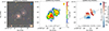 |
Fig. A.1. AHCJ140812.8+354433 as an example of a clear merged detection with two distinct optical counterparts within a well-resolved H I detection. Left: PanSTARRS1 color image overlaid with H I contours. Middle: S/N map of the H I detection. Right: Velocity field of the H I detection. All panels are obtained from the output of SIP. |
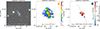 |
Fig. A.2. AHCJ120231.7+614724. Unclear merged detection with two distinct optical counterparts within a poorly resolved (with respect to the projected distance of optical counterparts) H I detection. Panels are the same as in Fig. A.1. |
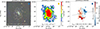 |
Fig. A.3. AHCJ123353.2+393735. Unclear merged detection with two distinct optical counterparts within a poorly resolved (with respect to the projected distance of optical counterparts) H I detection. Panels are the same as in Fig. A.1. |
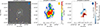 |
Fig. A.4. AHCJ131401.5+552253. Unclear merged detection with two distinct optical counterparts within a poorly resolved (with respect to the projected distance of optical counterparts) H I detection. Panels are the same as in Fig. A.1. |
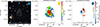 |
Fig. A.5. AHCJ222934.9+511016. Unclear merged detection with two distinct optical counterparts within a poorly resolved (with respect to the projected distance of optical counterparts) H I detection. Panels are the same as in Fig. A.1. |
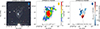 |
Fig. A.6. AHCJ235942.6+342048. Unclear merged detection with two distinct optical counterparts within a poorly resolved (with respect to the projected distance of optical counterparts) H I detection. Panels are the same as in Fig. A.1. |
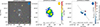 |
Fig. A.7. AHCJ120107.6+544859. Unclear merged detection with two distinct optical counterparts within a low S/N and poorly resolved (with respect to the projected distance of optical counterparts) H I detection. Panels are the same as in Fig. A.1. |
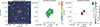 |
Fig. A.8. AHCJ232356.9+481659. Unclear merged detection with two distinct optical counterparts within a low S/N and poorly resolved (with respect to the projected distance of optical counterparts) H I detection. Panels are the same as in Fig. A.1. |
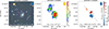 |
Fig. A.9. AHCJ024158.7+410448. Unclear merged detection with one clear optical counterpart and another (small) potential counterpart (in the northeast) within a low S/N H I detection. Panels are the same as in Fig. A.1. |
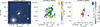 |
Fig. A.10. AHCJ143904.6+380854. Unclear merged detection with one clear optical counterpart and another (small) potential counterpart (in the southwest) within a low S/N H I detection. Panels are the same as in Fig. A.1. |
All Tables
All Figures
|
Fig. 1. Selection of dwarf galaxy samples from Apertif. The flowchart denotes most relevant steps in our selection procedure beginning from the Apertif source list to the dwarf galaxy samples used in this work. Boxes with bold text denote final samples used in our analysis. |
| In the text | |
|
Fig. 2. Properties of the parent dwarf galaxy sample. Left: histograms of H I (blue) and stellar (orange) masses of the sample. The vertical line denotes the dwarf stellar mass limit of 5 × 10⁹ M⊙. Right: systemic velocity vs. stellar mass of dwarfs in the sample, color-coded by the gas fraction. We show typical stellar mass error in the upper left corner. The vertical line is the same as in the left plot. On the right, we plot the histogram along the Vsys axis of our sample. |
| In the text | |
|
Fig. 3. Sketch of the classification of multiples. For simplicity, we show a case where all galaxies have the same stellar mass. The three galaxies are denoted with numbers one to three, and the selection criteria (both spatial and spectral) for companions are visualized as dashed (for galaxies 1 and 3) and dotted circles (for galaxy 2), centered at each galaxy. In this case, the number of companions is one for both galaxy 1 and 3, and two for galaxy 2. We classify this system as a triplet. |
| In the text | |
|
Fig. 4. Comparison of galaxy properties between the isolated and non-isolated subsamples of our parent dwarf sample. Left: M⋆–MH I relation. Isolated galaxies are plotted as purple squares, and non-isolated as orange circles. The error bars represent the median values and percentile errors, with the isolated sample shown as full purple lines, and non-isolated as dashed orange lines. The vertical black line denotes the stellar mass limit of 5 × 10⁹ M⊙. Right: M⋆–SFR relation. The markings are the same as in the left panel. |
| In the text | |
|
Fig. 5. Mean number of companions (of any stellar mass) per dwarf galaxy in the logarithmic stellar mass bin, normalized by the number of dwarfs in the same mass bin. Values represent the mean between different realizations of the sample in each mass bin. The black line represents results obtained using constant thresholds in projected distance and systemic velocity difference (150 kpc and 150 km s−1, respectively) for selection of companions, while the blue line represents results obtained using the mass-scaled thresholds (see Sect. 4.1). Both lines represent results for the total drawn dwarf galaxy sample. Shaded regions and error bars represent 1σ errors. |
| In the text | |
|
Fig. 6. Mean number of companions (of any stellar and/or baryonic mass) per dwarf in logarithmic stellar (left) or baryonic (right) mass bins, normalized by the number of dwarfs per bin. Values represent the median between different realizations of the sample in each mass bin. All lines are obtained using mass-scaled thresholds (see Sect. 4.1): the blue line represents the total drawn dwarf galaxy sample, the dashed purple line the isolated drawn sample including split multiples (upper limit), and the dotted pink line the isolated drawn sample excluding split multiples (lower limit). Shaded regions and error bars indicate 1σ uncertainties. The number of galaxies in each bin is shown at the top, with font colors and order matching the corresponding lines in the legend. |
| In the text | |
|
Fig. 7. Difference in the SFRs of paired galaxies with respect to the unpaired control sample vs. the pair separation scaled by the virial radius of the pair. Left: pairs with stellar mass ratios below 1/3. Primaries correspond to the more massive galaxy in a pair and are denoted by blue squares, while secondaries (the less massive in a pair) are denoted by red circles. Blue and red lines correspond to the running means for primaries and secondaries, respectively, with 1σ errors on the means denoted as shaded regions. Horizontal dashed and dotted black lines denote the 1σ and 2σ scatter of unpaired galaxies. Right: pairs with stellar mass ratios above 1/3. The notation is the same as in the left panel, except that the running mean (black line) is calculated by taking primary and secondary galaxies together. |
| In the text | |
|
Fig. 8. Comparison of the mean number of companions per dwarf between the Apertif and the SDSS samples. Left: case with no constraint on the projected radius between companions in Apertif. The blue line represents the result for the total drawn galaxy sample; the dotted pink represents the results from the isolated drawn sample by taking the lower limit (see Sect. 5.1); and the dashed orange line represents results from B18. Shaded regions represent 1σ errors. Right: same as in the left panel, but excluding all companions in Apertif for which rp < 55″. |
| In the text | |
|
Fig. 9. Flux distributions for galaxies found in merged detections (red) vs. separate detections (cyan) in our parent dwarf galaxy sample. Histograms are normalized to the number of galaxies in each sample (reported in the legend). The vertical dashed black line denotes the flux limit of 0.187 Jy km s−1 below which there is an excess of galaxies detected in merged detections. |
| In the text | |
|
Fig. 10. Mean number of companions (of any stellar mass) per dwarf in the logarithmic stellar mass bin, normalized by the number of dwarfs in the same mass bin. Values represent the median between different realizations of the sample in each mass bin. The blue line represents results for the total drawn dwarf galaxy sample, and the dotted gray line represents the results obtained by excluding all sources below the 0.187 Jy km s−1 threshold in the H I flux. Shaded regions represent 1σ errors. |
| In the text | |
|
Fig. A.1. AHCJ140812.8+354433 as an example of a clear merged detection with two distinct optical counterparts within a well-resolved H I detection. Left: PanSTARRS1 color image overlaid with H I contours. Middle: S/N map of the H I detection. Right: Velocity field of the H I detection. All panels are obtained from the output of SIP. |
| In the text | |
|
Fig. A.2. AHCJ120231.7+614724. Unclear merged detection with two distinct optical counterparts within a poorly resolved (with respect to the projected distance of optical counterparts) H I detection. Panels are the same as in Fig. A.1. |
| In the text | |
|
Fig. A.3. AHCJ123353.2+393735. Unclear merged detection with two distinct optical counterparts within a poorly resolved (with respect to the projected distance of optical counterparts) H I detection. Panels are the same as in Fig. A.1. |
| In the text | |
|
Fig. A.4. AHCJ131401.5+552253. Unclear merged detection with two distinct optical counterparts within a poorly resolved (with respect to the projected distance of optical counterparts) H I detection. Panels are the same as in Fig. A.1. |
| In the text | |
|
Fig. A.5. AHCJ222934.9+511016. Unclear merged detection with two distinct optical counterparts within a poorly resolved (with respect to the projected distance of optical counterparts) H I detection. Panels are the same as in Fig. A.1. |
| In the text | |
|
Fig. A.6. AHCJ235942.6+342048. Unclear merged detection with two distinct optical counterparts within a poorly resolved (with respect to the projected distance of optical counterparts) H I detection. Panels are the same as in Fig. A.1. |
| In the text | |
|
Fig. A.7. AHCJ120107.6+544859. Unclear merged detection with two distinct optical counterparts within a low S/N and poorly resolved (with respect to the projected distance of optical counterparts) H I detection. Panels are the same as in Fig. A.1. |
| In the text | |
|
Fig. A.8. AHCJ232356.9+481659. Unclear merged detection with two distinct optical counterparts within a low S/N and poorly resolved (with respect to the projected distance of optical counterparts) H I detection. Panels are the same as in Fig. A.1. |
| In the text | |
|
Fig. A.9. AHCJ024158.7+410448. Unclear merged detection with one clear optical counterpart and another (small) potential counterpart (in the northeast) within a low S/N H I detection. Panels are the same as in Fig. A.1. |
| In the text | |
|
Fig. A.10. AHCJ143904.6+380854. Unclear merged detection with one clear optical counterpart and another (small) potential counterpart (in the southwest) within a low S/N H I detection. Panels are the same as in Fig. A.1. |
| In the text | |
Current usage metrics show cumulative count of Article Views (full-text article views including HTML views, PDF and ePub downloads, according to the available data) and Abstracts Views on Vision4Press platform.
Data correspond to usage on the plateform after 2015. The current usage metrics is available 48-96 hours after online publication and is updated daily on week days.
Initial download of the metrics may take a while.