| Issue |
A&A
Volume 703, November 2025
|
|
|---|---|---|
| Article Number | A158 | |
| Number of page(s) | 37 | |
| Section | Cosmology (including clusters of galaxies) | |
| DOI | https://doi.org/10.1051/0004-6361/202554908 | |
| Published online | 28 November 2025 | |
KiDS-Legacy: Cosmological constraints from cosmic shear with the complete Kilo-Degree Survey⋆
1
Ruhr University Bochum, Faculty of Physics and Astronomy, Astronomical Institute (AIRUB), German Centre for Cosmological Lensing, 44780 Bochum, Germany
2
School of Mathematics, Statistics and Physics, Newcastle University, Herschel Building, NE1 7RU Newcastle-upon-Tyne, UK
3
Center for Theoretical Physics, Polish Academy of Sciences, al. Lotników 32/46, 02-668 Warsaw, Poland
4
Institute for Astronomy, University of Edinburgh, Blackford Hill, Edinburgh EH9 3HJ, UK
5
Leiden Observatory, Leiden University, P.O. Box 9513 2300 RA, Leiden, The Netherlands
6
Department of Physics and Astronomy, University College London, Gower Street, London WC1E 6BT, UK
7
Argelander-Institut für Astronomie, Universität Bonn, Auf dem Hügel 71, D-53121 Bonn, Germany
8
Institute for Computational Cosmology, Ogden Centre for Fundament Physics – West, Department of Physics, Durham University, South Road, Durham DH1 3LE, UK
9
Centre for Extragalactic Astronomy, Ogden Centre for Fundament Physics – West, Department of Physics, Durham University, South Road, Durham DH1 3LE, UK
10
Waterloo Centre for Astrophysics, University of Waterloo, Waterloo, ON N2L 3G1, Canada
11
Department of Physics and Astronomy, University of Waterloo, Waterloo, ON N2L 3G1, Canada
12
Institute for Theoretical Physics, Utrecht University, Princetonplein 5, 3584CC Utrecht, The Netherlands
13
Kapteyn Astronomical Institute, University of Groningen, PO Box 800 9700 AV, Groningen, The Netherlands
14
Institut de Física d’Altes Energies (IFAE), The Barcelona Institute of Science and Technology, Campus UAB, 08193 Bellaterra (Barcelona), Spain
15
School of Mathematics, Statistics and Physics, Newcastle University, Herschel Building, NE1 7RU Newcastle-upon-Tyne, UK
16
Centro de Investigaciones Energéticas, Medioambientales y Tecnológicas (CIEMAT), Av. Complutense 40, E-28040 Madrid, Spain
17
Institute of Cosmology & Gravitation, Dennis Sciama Building, University of Portsmouth, Portsmouth PO1 3FX, United Kingdom
18
Dipartimento di Fisica e Astronomia “Augusto Righi” – Alma Mater Studiorum Università di Bologna, Via Piero Gobetti 93/2, 40129 Bologna, Italy
19
INAF-Osservatorio di Astrofisica e Scienza dello Spazio di Bologna, Via Piero Gobetti 93/3, 40129 Bologna, Italy
20
Universität Innsbruck, Institut für Astro- und Teilchenphysik, Technikerstr. 25/8, 6020 Innsbruck, Austria
21
The Oskar Klein Centre, Department of Physics, Stockholm University, AlbaNova University Centre, SE-106 91 Stockholm, Sweden
22
Imperial Centre for Inference and Cosmology (ICIC), Blackett Laboratory, Imperial College London, Prince Consort Road, London SW7 2AZ, UK
23
Department of Physics, University of Oxford, Denys Wilkinson Building, Keble Road, Oxford OX1 3RH, UK
24
Donostia International Physics Center, Manuel Lardizabal Ibilbidea, 4, 20018 Donostia, Gipuzkoa, Spain
25
Zentrum für Astronomie, Universitatät Heidelberg, Philosophenweg 12, D-69120 Heidelberg, Germany; Institute for Theoretical Physics, Philosophenweg 16, D-69120 Heidelberg, Germany
26
Istituto Nazionale di Fisica Nucleare (INFN) – Sezione di Bologna, viale Berti Pichat 6/2, I-40127 Bologna, Italy
27
Department of Physics “E. Pancini” University of Naples Federico II C.U. di Monte Sant’Angelo Via Cintia, 21 ed. 6, 80126 Naples, Italy
28
INAF – Osservatorio Astronomico di Padova, via dell’Osservatorio 5, 35122 Padova, Italy
29
Institute for Particle Physics and Astrophysics, ETH Zürich, Wolfgang-Pauli-Strasse 27, 8093 Zürich, Switzerland
⋆⋆ Corresponding author: This email address is being protected from spambots. You need JavaScript enabled to view it.
Received:
31
March
2025
Accepted:
31
July
2025
Abstract
We present cosmic shear constraints from the completed Kilo-Degree Survey (KiDS), where the cosmological parameter S8 ≡ σ8√Ωm/0.3 = 0.81+0.016−0.021 is found to be in agreement (0.73σ) with results from the Planck Legacy cosmic microwave background experiment. The final KiDS footprint spans 1347 square degrees of deep nine-band imaging across the optical and near-infrared (NIR), along with an extra 23-square degrees of KiDS-like calibration observations of deep spectroscopic surveys. Improvements in our redshift distribution estimation methodology, combined with our enhanced calibration data and multi-band image simulations, allowed us to extend our lensed sample out to a photometric redshift of zB ≤ 2.0. Compared to previous KiDS analyses, the increased survey area and redshift depth results in a ∼32% improvement in constraining power in terms of Σ8 ≡ σ8(Ωm/0.3)α = 0.821+0.014−0.016, where α = 0.58 has been optimised to match the revised degeneracy direction of σ8 and Ωm for our current survey at higher redshift. We adopted a new physically motivated intrinsic alignment (IA) model that jointly depends on the galaxy sample’s halo mass and spectral type distributions, and which is informed by previous direct alignment measurements. We also marginalised over our uncertainty on the impact of baryon feedback on the non-linear matter power spectrum. Compared to previous KiDS analyses, we conclude that the increase seen in S8 primarily results from our improved redshift distribution estimation and calibration, as well as a new survey area and improved image reduction. Our companion paper presents a full suite of internal and external consistency tests (including joint constraints with other datasets), finding the KiDS-Legacy dataset to be the most internally robust sample produced by KiDS to date.
Key words: cosmology: observations / galaxies: photometry / gravitational lensing: weak / surveys
We dedicate this article to the memory of Nick Kaiser. He turned weak lensing into a powerful and practical cosmology probe, inspiring us to conceive the Kilo-Degree Survey. The KiDS project has relied greatly on his brilliant and wide-ranging foundational work.
© The Authors 2025
 Open Access article, published by EDP Sciences, under the terms of the Creative Commons Attribution License (https://creativecommons.org/licenses/by/4.0), which permits unrestricted use, distribution, and reproduction in any medium, provided the original work is properly cited.
This article is published in open access under the Subscribe to Open model. This email address is being protected from spambots. You need JavaScript enabled to view it. to support open access publication.
1. Introduction
Our current understanding of the large-scale structure (LSS) of the Universe, obtained over the last three decades thanks to increasingly sophisticated astronomical observations, can be regarded as one of the great successes of modern scientific inquiry. Detailed observations of the LSS probe fundamental physics, since the structures we observe were formed by an interplay of physical effects. These primarily include the self-gravity of matter, cosmic expansion, astrophysical feedback processes, and the repulsive effect of the cosmological constant or dark energy.
When it comes to understanding the growth and evolution of LSS, the cosmological stage is set by observations of the cosmic microwave background (CMB) that reveal the structure of dark and baryonic matter at early times. Together with other probes, including big-bang nucleosynthesis (BBN) and baryon-acoustic oscillations (BAOs), the CMB has been used to establish and tightly constrain the so-called standard model of cosmology, ΛCDM. It is a strikingly simple model based on only a handful of numerical parameters (Planck Collaboration VI 2020; Qu et al. 2024; Ge et al. 2025) and characterised, in particular, by two components that are at the origin of its name: a cosmological constant (Λ, which dominates the energy landscape at late times) and a cold dark matter (CDM) component that is dominant over baryonic matter by a factor of roughly five. Observations of the CMB constrain the parameters of this model at high redshift (z ∼ 1100), when the Universe was approximately 370 thousand years old. However, the model can be subsequently used to predict the properties of the LSS at late times (z ≲ 2; an extrapolation over more than 10 billion years), which can then be tested with low-redshift probes of cosmic structures.
Of the low-redshift probes, the relative prevalence of CDM poses a problem for those that rely on luminous tracers, such as galaxy clustering measurements. Modelling and constraining the relationship between luminous and dark matter (DM), also known as galaxy bias, constitutes one of the major systematic challenges of such measurements. In contrast, observations of the weak gravitational lensing effect of the LSS are intrinsically sensitive to all matter (dark or otherwise), eliminating the systematic uncertainty of galaxy bias. This unique feature has turned such ‘cosmic shear’ experiments into a major cosmological probe that is just entering its golden age. Indeed, it is the combination of cosmic shear with galaxy clustering – and their cross-correlation called galaxy-galaxy lensing (GGL) – that will potentially yield the most precise test of the standard model.
Over the past decade, the comparison between observations of low-z LSS and their CMB-based predictions has revealed a tension in the  parameter. Therefore, it has been the focus of extensive study. All contemporary cosmic shear measurements to date, except one, have yielded values of S8 that are lower than CMB predictions, indicating a universe with less structure and/or matter. The significance of these measurements varies, but there is a clear tendency towards lower values in the cosmic shear results of the past decade. Only the Deep Lens Survey (DLS; Jee et al. 2016) has reported a value that is higher than that of Planck, and even then only slightly. In contrast, lower values have been reported by the Canada-France-Hawaii Telescope Lensing Survey (CFHTLenS; Heymans et al. 2013), as well as from previous results from the ongoing ‘stage-III’ surveys by the Kilo-Degree Survey (KiDS; Asgari et al. 2021; Li et al. 2023a), the Dark Energy Survey (DES; Amon et al. 2022; Secco et al. 2022), the Hyper-Suprime Camera survey (HSC; Li et al. 2023b; Dalal et al. 2023), and a joint analysis by Dark Energy Survey and Kilo-Degree Survey Collaboration (2023). Other low-z LSS probes typically also share this trend but again with a varying level of significance (see Abdalla et al. 2022, for an overview).
Cosmic shear probes relatively low redshifts, and relatively small scales compared to other probes of LSS (see e.g. Figure 1 of Broxterman & Kuijken 2024, for a graphical summary). This makes cosmic shear somewhat more sensitive than other low-z probes to non-linear structure formation and astrophysical effects: the latter mainly involve feedback processes driven by supernovae and active galactic nuclei, collectively referred to below as baryonic feedback. It has therefore been suggested that inaccuracies in the modelling of non-linear scales might be the reason for the tension in S8, rather than a more fundamental cosmological cause (Yoon et al. 2019; Yoon & Jee 2021; Amon & Efstathiou 2022; Preston et al. 2023).
A definitive answer to the reality of the S8 tension is within reach. Currently, three stage-III surveys have finished their observations and are preparing their final analyses; one of which we present here. The next generation of surveys, called stage-IV, are just beginning, represented by the ESA Euclid mission (Euclid Collaboration: Mellier et al. 2025), the Legacy Survey of Space and Time (LSST) conducted with the Vera C. Rubin Observatory (Ivezić et al. 2019), the NASA Roman Space Telescope (Spergel et al. 2015), and the Chinese Space Station Optical Survey (Gong et al. 2019). We note that Euclid is expected to yield first cosmologically relevant results in 2026. These stage-IV surveys will soon provide datasets capable of measuring the growth of structure at low z with unprecedented precision.
New facilities and new instruments invariably bring along new challenges owing to, for instance, the novelty of their hardware. Comparatively, the final (usually called ‘legacy’) releases of a survey typically represent the culmination of years or decades of analysis, understanding, and refinement regarding their survey and the associated data. As such, the final releases of stage-III surveys will provide a crucial insight and reference for subsequent lensing studies of LSS with stage-IV surveys.
Here, we present the cosmic shear analysis of the completed Kilo-Degree Survey (KiDS) based on the fifth and final data release (KiDS-DR5; Wright et al. 2024), dubbed KiDS-Legacy. With extensive wavelength coverage enabled by its unique pairing with its near-infrared (NIR) sister survey VIKING (VISTA Kilo-Degree Infrared Galaxy Survey) and with its superb image quality in the r-band, KiDS is the stage-III survey that is arguably most suited to simultaneously leverage high-redshift galaxies and accurately calibrate their redshift distributions. Over the past decade, KiDS has been pushing to increasingly high redshifts, while continuously improving the redshift calibration, shear measurements, shear calibration through image simulations, and methodology to accurately extract cosmological constraints from the imaging data.
This paper represents the culmination of these efforts, providing the most robust and precise analysis of KiDS to date. Our dataset is the largest analysed by KiDS thus far (Sect. 3.1), utilising the most extensive spectroscopic redshift compilation prepared for any cosmic shear analysis (Sect. 3.2), and has been calibrated using the most sophisticated simulations produced for this purpose (Sect. 3.4). Improvements in methodology (Sect. 2) have allowed us to access the highest redshifts (with the most tomographic bins) studied for cosmic shear to date (Sect. 3.4). An efficient workflow for this study was enabled by the new COSMOPIPE analysis framework, which we have also made publicly available. We present null tests of our dataset in Sect. 4. The cosmological results are presented in Sect. 5, discussed in Sect. 6, and summarised in Sect. 7. Additionally, we include supplementary information regarding our power spectrum emulation (Appendix A), on the definition of parameters for our fiducial intrinsic alignment model (Appendix B), construction of band power spectra (Appendix C), covariance validation (Appendix D), Bn-mode exploration (Appendix E), correlation function cosmological analyses (Appendix F), detailed posterior analyses (Appendix G), tables of cosmological constraints (Appendix H), and details of changes made to the analysis and manuscript post-unblinding (Appendix I). Finally, this paper has been released alongside two companion papers: the work of Stölzner et al. (2025) presents an extensive analysis of internal and external consistency tests of the KiDS-Legacy dataset (including joint constraints with other datasets) and the work of Wright et al. (2025) describes the various redshift distribution and bias estimation developments made for KiDS-Legacy.
2. Modelling and theoretical framework
The main cosmic shear observable is the ellipticity correlation between pairs of galaxies. The signal depends on the two-point statistics of the shear and galaxy intrinsic alignment fields, which both trace the matter distribution and therefore depend on cosmological information. For our predictions and sampling, we used COSMOSIS, a modular cosmology pipeline described in Zuntz et al. (2015). We included a number of new and/or modified modules in our analysis, including a COSMOPOWER emulator for non-linear power spectra (Appendix A) and new intrinsic alignment models (Sect. 2.4). In this section, we start with the derivation of cosmic shear power spectra from matter power spectra and then detail our choices of intrinsic alignment models. Next, we introduce our observable two-point statistics, briefly discussing their measurement and prediction methodology. We end this section with a brief review of our analytical covariance modelling.
2.1. Shear power spectrum
Our two-point statistic predictions are calculated from shear (cross-)power spectra of galaxy samples i and j,  , where G stands for ‘gravitational’, which distinguishes these power spectra from intrinsic alignment contributions to the two-point signal. Shear power spectra are given by Limber-approximated projections (Kaiser 1992; LoVerde & Afshordi 2008; Kilbinger et al. 2017) taking the form
 (1)
(1)
where Pm, nl is the non-linear matter power spectrum and fK(χ) is the comoving angular diameter distance. Although the integral in Eq. (1) technically runs over the entire line of sight to the horizon, χhor, in practice, the weak lensing kernel,  , limits the integral to the comoving distance of the furthest galaxy in our sample, expressed as
 (2)
(2)
where  is the distribution of comoving distances of galaxies in source sample, i; in practice, we express this in terms of redshift, namely, N(z) dz = nS(χ) dχ. Here, Ωm is the total matter density parameter today, H0 is the Hubble constant, c is the speed of light, and a(χ) is the scale factor normalised to unity today.
2.2. Matter power spectrum
In our cosmic shear analysis, we remained mostly sensitive to Fourier scales 0.1 h/Mpc ≲ k ≲ 1 h/Mpc, with a weighting of scales that depends on the two-point statistic (see Sect. 2.5). These scales are well within the (quasi-) non-linear regime and therefore require an accurate non-linear power spectrum model for their predictions. Currently, there are multiple approaches that can produce non-linear matter power spectra, with varying levels of accuracy, for this range of scales. Here, we followed the most popular approach for cosmic shear analyses, using a method inspired by the halo model and calibrated against simulations. Specifically, we used the Boltzmann solver CAMB (Lewis et al. 2000; Howlett et al. 2012) to estimate the linear matter power spectrum and the augmented halo model ‘HMCODE2020’ (Mead et al. 2021) to derive its non-linear evolution.
HMCODE2020 has a similar level of accuracy as popular emulators trained directly on N-body simulations (2.5%; see e.g. Knabenhans et al. 2023; Aricò et al. 2021) and is twice as accurate as HALOFIT from Takahashi et al. (2012), which has been used in a number of previous cosmic shear analyses (see e.g. Amon et al. 2022; Hikage et al. 2019). Dark Energy Survey and Kilo-Degree Survey Collaboration (2023) presented a comparison of HMCODE2020 and HALOFIT with EUCLIDEMULATORV2, showing that HMCODE2020 produces unbiased results when analysing mock data created with EUCLIDEMULATORV2; meanwhile HALOFIT tends to overestimate power for lower values of S8, resulting in an underestimated S8 value. Similarly, an earlier version of HMCODE, HMCODE2015 (Mead 2015), which was used in previous KiDS analyses, is ∼30% less accurate than HMCODE2020. This can subsequently produce small differences between cosmological constraints estimated using the two codes: Tröster et al. (2021) demonstrated that the most important difference between these versions of HMCODE is in their treatment of baryon feedback, which results in a slightly higher S8 using HMCODE2020. Lastly, we note that the parameter values at which HMCODE was fitted to simulations are somewhat more constrained than our chosen priors for h2Ωm(see Mead et al. 2021, and Table 3). However, given that the fitting functions of HMCODE are based on physically motivated parameters, we did not anticipate any significant issues just beyond this range. Furthermore, we note that our analysis remained unaffected by this choice.
2.3. Baryonic feedback
The primary features of the matter power spectrum can be determined by assuming all matter is in the form of (pressureless) CDM, with modifications due to processes involving baryonic matter. At large scales (0.05 h/Mpc ≲ k ≲ 0.5 h/Mpc), BAOs produce oscillations in the power spectrum. Over a wide range of intermediate scales (0.1 h/Mpc ≲ k ≲ 10 h/Mpc), power is suppressed through feedback processes from active galactic nuclei (AGN), reaching a maximum suppression at around k ∼ 5 h/Mpc. At even smaller scales (k ≳ 10 h/Mpc), star formation processes lead to a sharp increase in power (see e.g. Semboloni et al. 2011).
To model baryonic feedback processes, HMCODE2020 performs a modification to the concentration-mass relation of the halo profiles as a function of their gas fraction; this, in turn, depends on the strength of the AGN feedback (parametrised by log(TAGN) ∈ [7.1,8.3]). This feedback model is then calibrated against a suite of hydrodynamical simulations from BAHAMAS (McCarthy et al. 2017), which had been generated using a wide range of effective feedback amplitudes and cosmological models. Recently, Schaye et al. (2023, FLAMINGO) presented a new suite of hydrodynamical simulations, including emulators for generating power spectra (Schaller et al. 2025), as a mechanism for modelling baryonic effects. Moving beyond hydrodynamical simulations, Salcido et al. (2023, SP(k)) presented alternative phenomenological models for the same purpose, while Schneider & Teyssier (2015), Aricò et al. (2020) presented perturbative models that act directly on the outputs of dark-matter only simulations and can be empirically calibrated (Grandis et al. 2024; Schneider et al. 2022). We did not utilise these models for our cosmological analyses here, as these models were published over the course of the analysis of KiDS-Legacy or were not (at time of writing) implemented within our COSMOSIS sampling framework. However, we note that a reanalysis of our data with these models is a natural and straightforward project that will be undertaken in a future publication.
2.4. Intrinsic alignments
The intrinsic alignment (IA) of galaxies is correlated with the observed ellipticities of galaxy images, making them indistinguishable from the cosmic shear effect we wish to probe for cosmological parameter estimation. In the limit of small shears and IA, the two-point statistics of galaxy ellipticities are given by
 (3)
(3)
where  is the cosmic shear signal given by Eq. (1). Analogous Limber equations can be derived for IA contributions, which are typically grouped into two categories. First, intrinsic-intrinsic (II) correlations represent the correlated alignment of galaxies that are tidally aligned by the same ambient LSS:
 (4)
(4)
Second, shear-intrinsic (GI) correlations are driven by the mutual gravitational effects of LSS on (i) galaxies within the structures, and (ii) the lensed images of background sources that these structures produce (Hirata & Seljak 2004):
 (5)
(5)
with  . In Eqs. (4) and (5) the power spectra PII, X and PδI, X are given by the chosen IA model. We note that the IA contributions feature a more compact kernel along the line of sight than the lensing kernel in Eq. (1), and hence the Limber approximation is poorer for these signals. However, this effect is not significant for our analysis, as the overall IA contributions to the total signal is small, making up only around 10 percent of the signal in our analysis. Additionally, we are only probing scales ℓ ≳ 50, where the Limber approximation is sufficient even for more compact kernels (Leonard et al. 2023).
Since IA are caused by the local matter environment, they have a different redshift scaling than lensing, which however is insufficient to isolate the cosmological signal without substantial information loss (Joachimi et al. 2008). Therefore, cosmic shear analyses opt for physically motivated IA models that are inferred jointly with the cosmology (see Lamman et al. 2024, for a review of the field). Guided by this, we implement four IA models in KiDS-Legacy: a widely used baseline with a single overall amplitude parameter (NLA, Sect. 2.4.1), two minimal extensions of NLA with either an additional redshift (NLA-z, Sect. 2.4.2) or scale dependence (via our restricted TATT model, NLA-k; Sect. 2.4.3), and a version of NLA that explicitly incorporates the well-established trends of IA with galaxy type and host halo mass (NLA-M, Sect. 2.4.4). The latter model is the fiducial model chosen for our cosmological analyses.
2.4.1. The non-linear linear alignment (NLA) model
The so-called NLA model (Bridle & King 2007) assumes that the intrinsic ellipticity of a galaxy depends linearly on its surrounding tidal quadrupole (Catelan et al. 2001). Moreover, it is commonly assumed that it is the tidal field at some early time during the formation of the galaxy that sets the amplitude of alignment (Hirata & Seljak 2004). This leads to the following expressions for the IA power spectra,
 (6)
(6)
where C1ρcr ≈ 0.0134 is a constant and D(z) is the linear growth factor normalised to unity at z = 0. The model is empirically extended to non-linear scales by employing the full, non-linear matter power spectrum Pm, nl, encapsulating a mixture of non-linear gravitational effects as well as alignment processes on the scales of dark matter halos (cf. Schneider & Bridle 2010). The model has a single free parameter, namely, the global, dimensionless amplitude AIA, which necessitates the assumption that there are no coherent trends in how galaxy ellipticities respond to their local tidal field within the survey’s galaxy population. Since AIA is well-constrained by tomographic cosmic shear data, we chose a wide top-hat prior for AIA to ensure its posterior is data-driven. All previous KiDS cosmic shear analyses have used the NLA model as their default and, to date, there has been no evidence that this simple prescription is insufficient in representing current-generation datasets (e.g. Dark Energy Survey and Kilo-Degree Survey Collaboration 2023).
2.4.2. Additional redshift dependence (NLA-z)
There is currently no observational evidence of redshift evolution in the amplitude of IA (Joachimi et al. 2011; Fortuna et al. 2021a), but the statistical uncertainties on measurements underpinning this statement are still large, especially when extrapolated to the redshift range of cosmic shear samples. Moreover, AIA could also acquire an effective redshift scaling; for example, due to a combination of a luminosity dependence and Malmquist bias. Hence, we tested whether the data prefer AIA to evolve over the tomographic bins. Since individual IA amplitudes per tomographic bin are poorly constrained (see the detailed analysis in Samuroff et al. 2019), we chose an extended model that is linear in terms of the scale factor,
![Mathematical equation: $$ \begin{aligned} P_{\delta \mathrm{I, zdep}}^{(i)}(k,z)&= - \left( A_{\rm IA} + B_{\rm IA} \left[ \frac{\langle a \rangle ^{(i)}}{a_{\rm piv}} -1 \right] \right) \frac{C_1 \rho _{\rm cr}\, \Omega _{\rm m}}{D (z)}\; P_{\rm m, nl}(k,z)\;, \\ \nonumber P_{\rm II, zdep}^{(ij)}(k,z)&= \left( A_{\rm IA} + B_{\rm IA} \left[ \frac{\langle a \rangle ^{(i)}}{a_{\rm piv}} -1 \right] \right)\\ \nonumber&\times \left( A_{\rm IA} + B_{\rm IA} \left[ \frac{\langle a \rangle ^{(j)}}{a_{\rm piv}} -1 \right] \right) \left( \frac{C_1 \rho _{\rm cr}\, \Omega _{\rm m}}{D (z)} \right)^2 P_{\rm m, nl}(k,z)\;, \end{aligned} $$](/articles/aa/full_html/2025/11/aa54908-25/aa54908-25-eq15.gif) (7)
(7)
where ⟨a⟩(i) is the average scale factor in tomographic bin i, evaluated using the estimated N(z). The parameter AIA thus is the IA amplitude at apiv ≈ 0.769, which corresponds to the commonly chosen pivot of z = 0.3 for IA studies (Joachimi et al. 2011). We set the prior range of the second parameter, BIA, by fitting our linear amplitude dependence to the compilation of KiDS and SDSS measurements studied in Fortuna et al. (2021a, see their Figure 10). Increasing the resulting constraint by 50 %, to account for the limited coverage of these calibration samples and for potential additional implicit redshift dependencies, we obtain a Gaussian prior on BIA with mean −3.7 and standard deviation 4.3. For direct comparisons between amplitudes estimated between this model and others, we define
 (8)
(8)
where  denotes the best-fitted (i.e. maximum a posteriori) value of each parameter.
2.4.3. Restricted TATT model (NLA-k)
By design, the angular scale dependence of the NLA model is identical to that of the matter power spectrum projected over the redshift distribution of the sample. A natural way to extend this is to consider next-to-linear alignment effects, specifically: (i) a density weighting (Hirata & Seljak 2004), accounting for the fact that alignments are only measured at local over-densities of the matter distribution where galaxies reside; and (ii) quadratic alignments as expected for tidal torquing effects (Crittenden et al. 2001; Catelan et al. 2001).
These contributions are subsumed into the tidal alignment, tidal torquing (TATT) model (Blazek et al. 2019), each with a free amplitude parameter. As can be seen from Figure 1 of Blazek et al. (2019), the density-weighting and quadratic terms have very similar dependence on physical scale. Owing to the scale-mixing of angular statistics, cosmic shear measurements poorly distinguish small and localised scale differences, which leads to pronounced degeneracies among the four TATT parameters (e.g. Samuroff et al. 2019). To avoid these, we implement the full TATT model within the analysis pipeline, but fix all but one of the free parameters that govern the non-linear terms. We treat this model as a more general modification to NLA, to capture potential deviations in scale from the model. We chose to keep the density weighting amplitude term free, thereby adding a single additional free parameter, but note that this choice is fairly inconsequential: given the aforementioned similarity between the scale dependence of the terms, implementing only the density weighting or only the quadratic term would produce a similar end product. The NLA-k model is then expressed as
![Mathematical equation: $$ \begin{aligned} \begin{aligned} P_{\delta \mathrm{I, scaledep}}(k,z)&= P_{\delta \mathrm{I, NLA}}(k,z)\\&\quad \!\!\!\!+ A_{\rm IA}\; b_{\rm src}\; \frac{C_1 \rho _{\rm cr}\, \Omega _{\rm m}}{D (z)}\; \left[ A_{0|0E}(k,z) + C_{0|0E}(k,z) \right]\;, \\ P_{\rm II, scaledep}(k,z)&= P_{\rm II, NLA}(k,z) \\&\quad \!\!\!\! + A_{\rm IA}^2 b_{\rm src}^2 \left( \frac{C_1 \rho _{\rm cr}\, \Omega _{\rm m}}{D (z)} \right)^2 A_{0\mathrm E|0\mathrm E}(k,z) \\&\quad \!\!\!\!+ 2\, A_{\rm IA}^2 b_{\rm src} \left( \frac{C_1 \rho _{\rm cr}\, \Omega _{\rm m}}{D (z)} \right)^2 \left[ A_{0|0\mathrm E}(k,z) + C_{0|0\mathrm E}(k,z) \right]\,, \end{aligned} \end{aligned} $$](/articles/aa/full_html/2025/11/aa54908-25/aa54908-25-eq18.gif) (9)
(9)
where the expressions for A0|0E, C0|0E, and A0E|0E are given in Blazek et al. (2019). We consider these terms in the Limber approximation where only transverse modes contribute, and assume that their redshift evolution is inherited from the linear matter power spectrum. In the original density-weighting term, the free parameter bsrc can be interpreted as an effective galaxy bias of the weak lensing source sample, albeit on fairly non-linear scales. For our model, we chose a top-hat prior in the range [ − 0.5, 1.5] to ensure it encompasses NLA (bsrc = 0) and reasonable values expected for the (unknown) source galaxy bias (bsrc ∼ 1). For comparisons between the alignment amplitude estimated with this model and others, we report the alignment amplitude of the NLA component of the model from Eq. (9), namely,
 (10)
(10)
2.4.4. Galaxy-type and mass-dependent model (NLA-M)
Two trends in IA strength are firmly established observationally: (i) a dichotomy between late- and early-type galaxies where only the latter have yielded significant detections on cosmological scales (Samuroff et al. 2023; Johnston et al. 2019; Heymans et al. 2013; Georgiou et al. 2025; see also Mandelbaum et al. 2011; Tonegawa et al. 2025; McCullough et al. 2024 for additional examples of null or marginal detections of late-type alignments); and (ii) a scaling of early-type alignment amplitude with host halo mass that is well described by a power-law (Joachimi et al. 2011; Fortuna et al. 2025). Both have solid theoretical underpinning. First, rotationally supported late-type galaxies are expected to align through tidal torquing, which depends quadratically on the tidal quadrupole, whereas spheroid shapes should respond linearly and thus be well described by NLA-like models. Second, Piras et al. (2018) motivated the halo mass dependence through an analytical argument and also reproduced it for simulated dark matter haloes.
We incorporated these IA trends explicitly into the amplitude of the NLA model. We assumed that, in each tomographic bin, only the fraction fr of ‘red’ (i.e. early-type) galaxies intrinsically align, whereas the remaining galaxies have zero alignment. The latter assumption is consistent with observations, but within a large statistical uncertainty and involving a substantial extrapolation in sample properties, primarily due to the imperfect relation between galaxy colour and rotational/pressure support (which is the property most-likely to cleanly stratify intrinsic alignment amplitudes). Moreover, we assumed that the red galaxy population IA amplitude has a power-law dependence on the average halo mass ⟨Mh⟩ within a tomographic bin. This leads to
 (11)
(11)
where we adopt the pivot halo mass Mh, piv = 1013.5 h−1 M⊙ from Fortuna et al. (2025). The same authors also fit the power-law dependence to a compilation of early-type IA measurements (see their Figure 4), and we adopt their joint posterior on AIA and β as our prior for cosmic shear inference. Their posterior is well approximated by a bivariate Gaussian with AIA = 5.74 ± 0.29, β = 0.44 ± 0.03, and a correlation coefficient of −0.59. Details on how we determine fr and halo masses for our sample of cosmic shear sources, and how we treat their associated uncertainties, are provided in Appendix B. For comparisons between the alignment amplitude estimated with this model and others, we define
 (12)
(12)
2.5. Cosmic shear summary statistics
In cosmic shear analyses, it is most convenient to measure the signal using shear two-point correlation functions (2PCFs) while the modelling is done through shear power spectra (see Eq. (1)). Alternatively, one could take the Fourier transform of the shear field and work in harmonic space, which brings the measurements closer to the theoretical predictions. We chose to use 2PCFs for the measurement, as they shield us from a particular form of E-/B-mode mixing that occurs in harmonic space in the presence of the (unavoidable) image masks. In addition, the shot-noise term does not impact 2PCFs (present only in their covariance), as it is only relevant at zero lag. In harmonic space, both shot noise and masking must be modelled and corrected, prior to beginning cosmological analyses. For more details see e.g. Alonso et al. (2019).
Our cosmological analysis here leverages two-point statistics: the complete orthogonal sets of E/B-integrals (COSEBIs, Sect. 2.5.2) and band power spectra (Sect. 2.5.3), constructed using linear combinations of finely-binned 2PCFs (Sect. 2.5.1).
2.5.1. 2PCFs (ξ±)
The shear two-point correlation functions (ξ±, Kaiser 1992) are functions of the tangential and cross components of shear (γt and γ×, respectively) defined with respect to the line connecting pairs of galaxies with angular separation θ (see e.g. Bartelmann & Schneider 2001),
 (13)
(13)
The measured 2PCFs are binned in θ to reduce measurement noise and compress the data. In practice, we measure ξ±(θ) for 1000 logarithmically spaced θ-bins between θmin = 2′ and θmax = 300′ using TREECORR1 (Jarvis et al. 2004). The inputs to TREECORR are galaxy catalogues, which include galaxy ellipticities (ε1 and ε2), galaxy positions (right ascension and declination), and galaxy weights (w). The weights used by TREECORR are equal to the recalibrated shape weights (Sect. 3.5) multiplied by the redshift distribution gold-weights (Sect. 3.4). Our ξ±(θ) are then estimated using
![Mathematical equation: $$ \begin{aligned} \hat{\xi }^{(ij)}_\pm (\bar{\theta })=\frac{\sum _{ab} w_a w_b \left[{\varepsilon }^\mathrm{obs}_{\mathrm{t},a}\,{\varepsilon }^\mathrm{obs}_{\mathrm{t},b} \pm {\varepsilon }^\mathrm{obs}_{\times ,a}\,{\varepsilon }^\mathrm{obs}_{\times ,b}\right] \Delta ^{(ij)}_{ab}(\bar{\theta }) }{\sum _{ab} w_a w_b (1+m_a)(1+m_b) \Delta ^{(ij)}_{ab}(\bar{\theta }) }\ , \end{aligned} $$](/articles/aa/full_html/2025/11/aa54908-25/aa54908-25-eq23.gif) (14)
(14)
where  is the bin selection function (which limits the sums to galaxy pairs of separation within the angular bin labelled by
  and the tomographic bins i and j), and
  and
and  are the projected tangential and radial components of observed ellipticities between pairs of galaxies. The estimator includes the galaxies’ multiplicative shear measurement biases ma estimated via image simulations (Sect. 3.4).
Using the flat-sky approximation, we can relate the 2PCFs to the angular (shear) power spectra by Hankel transformations:
![Mathematical equation: $$ \begin{aligned} \xi _\pm ^{(ij)}(\theta )&= \int _0^\infty \frac{ \ell \mathrm{d} \ell }{2 \pi } \; \left[C^{(ij)}_{{\varepsilon }{\varepsilon },\mathrm{E} }(\ell ) \pm C^{(ij)}_{{\varepsilon }{\varepsilon },\mathrm{B} }(\ell )\right] \; {\mathrm{J} }_{0/4}(\ell \theta )\;, \end{aligned} $$](/articles/aa/full_html/2025/11/aa54908-25/aa54908-25-eq28.gif) (15)
(15)
where  are the E/B-mode angular power spectra for redshift bins i and j, and J0/4(x) are the zeroth- and fourth-order Bessel functions of the first kind. We expect cosmic shear to produce only E-mode signals up to first order (Schneider et al. 1998; Hilbert et al. 2009), while data systematic errors can in principle create both E and B modes. As a result, B-modes have long been used as a diagnostic tool in cosmic shear analyses (see e.g. Pen et al. 2002; Hoekstra et al. 2002; Heymans et al. 2005; Kilbinger et al. 2013).
As ξ± mix E and B modes, they are not ideal for cosmic shear analysis. In addition, they variably weight a large range of physical scales in each angular bin, increasing sensitivity to scale-dependent effects such as baryonic feedback (which must be marginalised over using imperfect models). Figure 1 shows the range of ℓ probed by the ξ± over a range of angular separations. The J0 filter in Eq. (15) means that ξ+ mixes a very wide range of scales (1 ≲ ℓ ≲ 104) and J4 makes ξ− particularly sensitive to smaller scales (10 ≲ ℓ ≲ 105). This breadth can create a problem when using ξ± for inference, as the power spectra and intrinsic alignment models become increasingly uncertain at smaller scales. Consequently, we expect the cosmological constraints to be possibly affected by a range of systematic effects that may introduce biases and, as such, we do not include ξ± in our primary cosmological analyses. Nevertheless, results for ξ± are provided for completeness and comparison with previous work, in Appendix F.
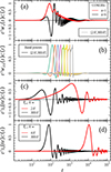 |
Fig. 1. Integrands of the transformation between the angular power spectrum and En/Bn (Eq. 17, panel ‘a’), CE, B (Eq. C.5, panel ‘b’), and ξ± (Eq. 15, panels ‘c’ and ‘d’). All solid integrands are normalised by their maximum absolute value. For both COSEBIs and 2PCFs, we show the limiting ranges of the statistics (n ∈ {1, 6} for En and θ ∈ {2.0, 300.0} arcmin for ξ±). For CE, B we show all eight bins used in KiDS-Legacy, defined between ℓ = 100 and ℓ = 1500. Note that, unlike previous KiDS analyses, our new treatment of T(θ) means that the CE, B initially go to zero within their desired ℓ ranges. |
2.5.2. COSEBIs (En/Bn)
The COSEBIs (Schneider et al. 2010) were originally designed to cleanly separate E- and B-modes over a finite θ-range. This was achieved through the use of filter functions T±n(θ), which form complete bases, creating well-defined COSEBIs E- and B-modes (En/Bn). COSEBIs can be calculated or measured via a linear transformation of ξ±,
![Mathematical equation: $$ \begin{aligned} \begin{aligned} \hat{E}_n&= \frac{1}{2} \int _{\theta _{\rm min}}^{\theta _{\rm max}} \mathrm{d}\theta \,\theta \, [T_{+n}(\theta )\,\xi _+(\theta ) + T_{-n}(\theta )\,\xi _-(\theta )]\;, \\ \hat{B}_n&= \frac{1}{2} \int _{\theta _{\rm min}}^{\theta _{\rm max}}\mathrm{d}\theta \,\theta \, [T_{+n}(\theta )\,\xi _+(\theta ) - T_{-n}(\theta )\,\xi _-(\theta )]\;. \end{aligned} \end{aligned} $$](/articles/aa/full_html/2025/11/aa54908-25/aa54908-25-eq30.gif) (16)
(16)
The COSEBIs modes n start from 1 and go to infinity. However, the first few COSEBIs are sufficient to capture essentially all the cosmological information in each pair of tomographic bins (Asgari et al. 2012). This means that COSEBIs naturally compress the data into well-defined modes, once θmin and θmax are defined, without any need for subsequent data compression. In previous KiDS analyses (e.g. Asgari et al. 2021), the first five COSEBIs modes were used for cosmological analyses. In this work, however, we add the sixth mode, as we found that (with our increased constraining power, and larger redshift baseline) the sixth mode contains relevant cosmological information and thus improves our constraining power on S8. Conversely, the addition of modes 7 − 20 did not result in any improvement of constraining power, returning constraints identical to those measured in the 6 mode case.
We use the relation between COSEBIs and shear power spectra to make our predictions,
 (17)
(17)
where the weight functions Wn(ℓ) are
 (18)
(18)
Figure 1 shows two example integrands from Eq. (17). Wn(ℓ) are highly oscillatory weight functions with a limited range of support over ℓ. This allows us to truncate our integrals in Eq. (17) to a finite range in ℓ, as the En integrand in Eq. (17) is practically zero outside 10 ≲ ℓ ≲ 103.
2.5.3. Band powers (CE, B)
Band power spectra (hereafter ‘band-powers’) refer to binned angular power spectra measured by integrating over ξ±(θ) (Schneider et al. 2002; van Uitert et al. 2016; Joachimi et al. 2021). Ideally, we want a finite number of bins, labelled as l, where each bin is only sensitive to a narrow range of ℓ-values between ℓlo, l and ℓup, l. We also want the E- and B-mode band-powers to be pure, namely, no leakage from B modes into E modes and vice versa. For this ideal case, we can express the following:
 (19)
(19)
for redshift bins i and j, where Sl(ℓ) is the response function for bin l. Here we have normalised the integral with
 (20)
(20)
In this work, we consider the ideal case of a top-hat response function between ℓlo, l and ℓup, l which simplifies the normalisation to
 (21)
(21)
and produces a band-power that traces ℓ2C(ℓ) at the logarithmic centre of the bin. We define eight band-powers logarithmically binned between ℓmin = 100 and ℓmax = 1500. In practice, measuring band-powers with perfect top-hat functions is infeasible, as ξ±(θ) is only measured for a finite θ-range. This has the adverse effect that our band-powers will inevitably mix E and B modes2. The mixing increases for narrower ℓ-bins and when the available range of θ-scales is smaller (Asgari & Schneider 2015). With this definition for band-powers, we forgo perfect E-/B-mode separation in favour of more control over the ℓ-values that contribute to our analyses. We present the detailed derivation of our band-power windows  in Appendix C, and show the integrands of
  in Fig. 1. Note, however, that our integrands behave differently to those in Asgari et al. (2021), due to our different treatment of the edges of T(θ) (Appendix C) and due to our different scale-cuts.
2.6. Analytic covariance modelling
We presented the covariance modelling for KiDS-Legacy and the ONECOVARIANCE code3 in Reischke et al. (2025). In general, the methodology for the cosmic shear part still follows closely the covariance modelling of KiDS-1000 (Joachimi et al. 2021). Major changes to the previous analysis include: (i) the possibility of including non-uniform source distributions in the mixed term of the covariance from the triplet counts of the survey; (ii) including non-binary masks for the area calculation and survey response; and (iii) offering a more generalised framework for a consistent treatment of all summary statistics used in KiDS-Legacy.
The cosmic shear covariance, C, generally consists of four contributions:
 (22)
(22)
with the Gaussian contribution G, the non-Gaussian term NG due to non-linear in-survey modes, the super-sample covariance SSC from modes larger than the survey, and lastly the contribution due to the uncertainty in the multiplicative shear bias calibration, Cmult. Asgari et al. (2021), Secco et al. (2022) included the multiplicative shear bias in the theory prediction instead and marginalised over in the sampling process. If the residual uncertainties on ma are small, these two approaches are equivalent. The Gaussian contribution can further be split into three parts:
 (23)
(23)
describing the sample variance term ‘sva’ due to the finite number of available modes in the survey volume, the pure shot noise term ‘sn’ due to the finite number of sources and their composition, and the mix term ‘mix’.
We calculated the covariances for angular power spectra and transform those to the three summary statistics considered. The only exception was the pure noise term, which was directly computed from the weighted number of pairs in the catalogue. SSC and NG terms were modelled with a halo model approach and the survey variance was directly calculated from the survey mask. Our analytical prescription was tested against GLASS (Tessore et al. 2023) mocks to test the impact of variable depth and the overall agreement. These mocks are discussed in more detail in Appendix D. In Reischke et al. (2025), we showed that the agreement between our analytic covariance and that constructed from GLASS is within 10 percent at large angular separations and below 5 percent for scales below 0.5 degrees. Furthermore, we found that our idealised mix term (which does not account for non-uniformity of the source distribution) did not affect our inference results significantly, and as a result was neglected in our analyses.
3. Data and analysis
In this section, we summarise the KiDS-Legacy lensing data and its calibration, the associated image simulations, and our analysis blinding strategy. Our analysis was performed using a new version of the COSMOPIPE infrastructure presented in Wright et al. (2020). Our fiducial pipeline includes all steps required for a catalogues-to-cosmology analysis, leveraging three primary inputs: a (blinded) shear catalogue (Sect. 3.3), a spectroscopic compilation (Sect. 3.2), and a simulated galaxy lightcone (Sect. 3.4). With these data products, the pipeline performs nine primary functions: pre-processing of the wide-field catalogue, simulated catalogue construction, redshift calibration, N(z) construction, shear calibration, data vector construction, covariance construction, cosmological inference, and post-processing. Details of each processing step are provided alongside the public code base4.
Figure 2 shows the footprint of the KiDS-Legacy sample, split between the two survey patches of KiDS (one in each of the northern and southern Galactic caps). The figure is coloured by the mean effective weight (i.e. including both shape measurement and redshift distribution estimation weights) of sources on sky, which is an approximate tracer of survey properties such as the size of the point-spread function and variable depth (see Appendix D and Yan et al. 2025). The weight is defined as described in Section 7 of Wright et al. (2024), and has the range ![Mathematical equation: $ w\in[0,\sigma_{\mathrm{pop}}^{-2}] $](/articles/aa/full_html/2025/11/aa54908-25/aa54908-25-eq40.gif) , where σpop = 0.255 is an approximate intrinsic ellipticity dispersion of all sources in KiDS (without e.g. tomographic or brightness selections) defined for Legacy in Li et al. (2023c).
, where σpop = 0.255 is an approximate intrinsic ellipticity dispersion of all sources in KiDS (without e.g. tomographic or brightness selections) defined for Legacy in Li et al. (2023c).
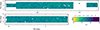 |
Fig. 2. Distribution of the mean weight of the KiDS-Legacy source galaxies in on-sky bins (0.1 × 0.1 degrees). The weights here include both shape measurement weights (Sect. 3.5) and redshift distribution gold weighting (Sect. 3.4). |
3.1. KiDS and VIKING
The KiDS-Legacy lensing sample was drawn from the fifth and final data release of the KiDS survey5, KiDS-DR5, described in Wright et al. (2024). It includes 1347 square-degree tiles observed in the u, g, r, and i filters with the VST (Capaccioli et al. 2005) and OmegaCAM (Kuijken 2011) between 2011 and 2019, as well as the 2009–2018 VIKING survey VISTA/VIRCAM observations (Edge et al. 2013) of the same area in Z, Y, J, H, and Ks. Additionally, the dataset contains spectroscopic calibration fields (the ‘KiDZ’ fields, 27 square-degree tiles in total, including four that are part of the main survey).
KiDS-DR5 significantly extends the previous (fourth) data release (Kuijken et al. 2019), which was the basis for the KiDS-1000 analyses (Asgari et al. 2021; Heymans et al. 2021; Tröster et al. 2021). It represents a substantial increase in survey area (by 34%) and in i-band depth (doubling the exposure time with a second pass). The volume of photometric redshift calibration data has also grown, including photometry for 5 times more spectroscopic sources than in the original KiDS-1000 analysis (Hildebrandt et al. 2021). The deeper i-band depth and more extensive calibration data has allowed us to push the photometric redshift limit for galaxies in the lensing sample from 1.2 to 2. The combined effect of the increase in area and depth is an increase in the survey volume of a factor of 3.5.
Several aspects of the data analysis were changed between DR4 and DR5, as detailed in Wright et al. (2024). The astrometry reference catalogue for the THELI reduction moved from the Sloan Digital Sky Survey (SDSS Ahumada et al. 2020) and the 2-micron All Sky Survey (2MASS Skrutskie et al. 2006) to Gaia DR2 (Gaia Collaboration 2018), and the astrometric solutions and photometric zero-point determinations in the ASTRO-WISE u-band reductions were made more robust. Also, the manual and automated masking of artefacts in the images, mostly due to ghost reflections, artificial satellite tracks, and detector instabilities, was revisited and improved for the final release. Most importantly, the weak lensing shape measurement method uses an updated version of lensfit (v321), with improvements in the sampling of the ellipticity likelihood surface and of the treatment of residual PSF leakage in the shapes and associated weights (Li et al. 2023c). Details and tests of these new implementations are given in Wright et al. (2024), and in the sections below. A summary of the properties of the KiDS-Legacy sample is given in Table 1, including details of tomographic bin limits, final effective number densities of galaxies (after redshift distribution calibration), and redshift and shape measurement bias parameters.
Properties of the six KiDS-Legacy tomographic bins.
Lastly, we note that a pernicious astrometric issue was identified during the investigation of our B-mode null tests (Sect. 4.3), which resulted in additional masking of approximately 4% of the survey sources to be used in the KiDS-Legacy analysis. More details are given in Sect. 4.3 and Appendix E. The total area after masking is 967.4 deg2, with neff = 8.79 per arcminute within the photometric redshift limits of KiDS-Legacy.
3.2. KiDZ
The KiDZ data consist of VST and VISTA images that target well-studied spectroscopic survey fields, including the Cosmic Evolutions Survey field (COSMOS; Scoville et al. 2007), the DEEP2 Galaxy Redshift Survey (DEEP2; Newman et al. 2013) 02h and 23h fields, the Chandra Deep Field South (CDFS), the Visible Multi-object Spectrograph (VIMOS) Very Large Telescope (VLT) Deep Survey (VVDS; Le Fèvre et al. 2005) 14h field, and the VIMOS Public Extragalactic Redshift Survey (VIPERS; Guzzo et al. 2014) W1 and W4 fields (a full list is given in Wright et al. 2024). They were purposely taken under very similar observing conditions, and with the same observing setup, as the main KiDS/VIKING survey and serve as the calibration sample for photometric redshifts of the faint KiDS sources. A total of 126 085 sources with spectroscopic redshifts have nine-band KiDZ photometry. Additional photometric redshift calibration via cross-correlations uses the overlap between KiDS and shallower, wide-angle spectroscopic redshift surveys, principally: SDSS, the Galaxy And Mass Assembly (Driver et al. 2022) survey, 2-degree Field Lensing Survey (Blake et al. 2016), WiggleZ survey (Blake et al. 2008), and the Dark Energy Spectroscopic Instrument (DESI Collaboration 2024).
3.3. Blinding
We used the same blinding methodology as the one implemented in Asgari et al. (2021), first presented in Kuijken et al. (2015). This process involves the double-blind generation of threerealisations of our shape measurement catalogues. One of these is the true catalogue, while in the other two there are induced systematic differences in measured shapes that result in (up to) ±2σ change in the inferred S8. The true catalogue is equally likely to be the one that yields the highest, middle, or lowest S8. These blinded data vectors were analysed throughout the project until the analyses were finalised, cosmological chains were run, the results written up in this publication, and the manuscripts had undergone internal review within the KiDS collaboration. As such, this manuscript (for example) was written containing results for all three blinds, with only the discussion and conclusion sections written afterunblinding.
The authors note (for the reference of future surveys) that this blinding scheme effectively hampered the diagnosis of subtle systematic effects in the dataset (see Appendix E), as we were limited in our ability to directly compare measured shapes between previously constructed catalogues and our KiDS-Legacy catalogues. Such comparisons are extremely useful for the validation of spatially localised systematic patterns in the shape catalogue, which are obfuscated when translated into two-point statistics. This blinding strategy, however, makes such direct comparisons between shape catalogues problematic, as it can also lead to unblinding.
3.4. Redshift distributions and calibration
Redshift distributions (hereafter ‘N(z)’) used in KiDS-Legacy were estimated and calibrated leveraging both colour-based direct calibration using self-organising maps (SOMs Kohonen 1982) and spatial cross-correlations (CC) between tracer spectroscopic samples and the KiDS-Legacy sources. For a detailed description of the N(z) construction and validation process used in this work, we refer to Wright et al. (2025). In brief, the N(z) here differ in their construction (compared to previous work from KiDS) in three main regards: a considerably larger redshift calibration sample from KiDZ (see Sect. 3.2); a new weighting scheme that replaces the binary ‘gold-class’ with a continuous ‘gold-weight’; and through the optional inclusion of weights for spectroscopic objects, such as our so-called ‘prior-volume weighting’. Gold-weights primarily account for noise in the colour-based association between wide-field sources and their calibrating spectra, and are computed by repeating the gold classification N times (where we arbitrarily chose N = 10). Similarly, our prior-volume weighting applies an a priori weighting to the distribution of calibrating spectra as a function of redshift, to reduce bias caused by colour-redshift degeneracies and the complex redshift selection function of our spectroscopiccompilation.
The redshift distribution calibration for KiDS-Legacy made use of two suites of simulations. For the calibration of the SOM redshift distributions (and calibration of source shape measurements, Sect. 3.5), we used the multi-colour SKiLLS simulation of Li et al. (2023c). For additional SOM redshift distribution calibration and cross-correlation redshift distribution calibration, we used the MICE2 simulated lightcone (Fosalba et al. 2015a; Crocce et al. 2015; Fosalba et al. 2015b; Carretero et al. 2015; Hoffmann et al. 2015) adapted to KiDS noise levels and sample selections (van den Busch et al. 2020).
Figure 3 shows the fiducial redshift distributions used in this cosmological analysis. These N(z) include the appropriate δz shifts in each of their mean, as inferred using our simulations and described in Wright et al. (2025). As such, the N(z) presented are shown as-used in the generation of the theory/models during parameter inference. In Wright et al. (2025) we quantified the impact of a series of different analysis choices for N(z) estimation and calibration, demonstrating that they have no significant impact on the final N(z) that we used for cosmological inference. The figure also presents the off-diagonal elements of the correlation matrices for δz, used to construct our correlated δz priors. The lower triangle shows the correlation matrix estimated from our SOM redshift distribution calibration, while the upper triangle shows the correlation matrix for the CC estimated redshift distributions.
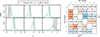 |
Fig. 3. Left:N(z) used in the fiducial cosmic shear analyses of KiDS-Legacy. Each panel is one tomographic bin whose definition is determined by the grey band in photo-z. The N(z) have been shifted according to the mean bias estimated using our SKiLLS simulations, making each N(z) a correct representation of the effective N(z) that is used in the cosmological analyses. Fiducial biases are provided in Table 1. Right:δz correlation matrix for our fiducial N(z) (δzSOM, lower triangle) and the correlation matrix inferred from our cross correlation N(z) on the data (DzCC, upper triangle). |
3.5. Shape measurement and calibration
The measurement and calibration of source shapes in KiDS-Legacy were performed with the latest KiDS methods, which have already been established in the literature. We refer to Li et al. (2023c) for an extensive description of the state-of-the-art for shape measurement and calibration in KiDS. Topics discussed therein include: the lensfit algorithm (v321; see also Miller et al. 2007, 2013; Fenech Conti et al. 2017), used for measuring shapes of galaxies (including modelling of the PSF); shape calibration using SKiLLS image simulations; and PSF leakage corrections (with minor updates to the PSF leakage estimation as described in Wright et al. 2024). The SKiLLS image simulations are multi-band image simulations, constructed specifically to match the observational properties of KiDS-Legacy in all available bands, and featuring realistic clustering and correlations between galaxy properties and environment, allowing for realistic treatment of blending effects. The simulations also feature redshift-dependent shear (MacCrann et al. 2022), although this is determined to be of negligible importance to the computation of multiplicative bias (Li et al. 2023c) and redshift distribution bias (Wright et al. 2025) at the sensitivity of KiDS-Legacy.
The multiplicative bias estimation in KiDS-Legacy was performed using the same suite of multi-colour image simulations from SKiLLS used for redshift distribution calibration. Redshift distribution calibration utilises many realisations of the sample to estimate uncertainties on tomographic bias parameters (see Wright et al. 2025). Afterwards, these samples were also used to estimate the multiplicative shear measurement bias, m, per tomographic bin. This means that, for the first time, we have been able to directly estimate the covariance between our redshift distribution bias calibration and our multiplicative shear bias estimation. The resulting covariance matrix (and the corresponding correlation matrix) are functionally block-diagonal: there is no cross covariance between m and δz estimates.
We checked for the degree of PSF leakage measured in the lensing sample through a direct empirical calculation of the correlation between PSF and galaxy ellipticities. Here, we document the measured PSF contamination in our KiDS-Legacy sample, and the measured residual one- and two-dimensional constant ellipticity terms (‘c-terms’) in the dataset. We adopted the first-order systematics model from Heymans et al. (2006):
 (24)
(24)
where k denotes the individual ellipticity components, γ is the (true) shear, and the superscripts ‘obs’, ‘int’, and ‘PSF’ refer to a source’s observed, intrinsic, and modelled PSF ellipticity, respectively. In the limit of large numbers of sources averaged over a large sky area, we can assume ⟨(1 + mk)(εkint + γk)⟩ = 0, and therefore model the residual PSF contamination using a simple linear regression between observed source ellipticities (i.e. after recalibration to remove PSF leakage Li et al. 2023c; Wright et al. 2024) and modelled PSF ellipticities.
Figure 4 shows the αk and ck PSF leakage terms in each ellipticity component of the KiDS-Legacy sample, measured in each tomographic bin. Note that the shape recalibration process used in KiDS-Legacy necessitates that the measured PSF leakage factors be approximately zero, as the recalibration specifically addresses any residual in this parameter, in bins of source signal-to-noise ratio (SN) and resolution (Li et al. 2023c). The residual αk are all negligible, with the α2 having a slightly larger residual amplitude overall (α2 ≈ 0.01, roughly three orders of magnitude smaller than that measured before any recalibration effort). Furthermore, we note that the constant term shown in the figure (ck) is not the same as the additive bias which is removed from our galaxy sample. In practice, the additive component of our ellipticities was computed directly (using a weighted mean) from the sample of galaxies per tomographic bin and hemisphere:  . The
. The  -terms that were subtracted from our recalibrated shape catalogues prior to computation of correlation functions are provided in Table 2. In contrast, the figure presents the constant component of our linear regression (Eq (24)) to all data per tomographic bin after removal of the additive bias. As such it is expected that the ck-terms are small, but not necessarily zero.
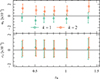 |
Fig. 4. PSF leakage measured in the KiDS-Legacy lensing sample after recalibration of shapes, computed per tomographic bin and ellipticity component k, and following the first-order systematics model in Eq. (24). |
Subtracted additive shear per ellipticity component, tomographic bin, and hemisphere.
As a further quality test, we computed the non-tomographic 2D c-terms in camera coordinates per ellipticity component, which is shown in Fig. 5. The 2D c-terms were calculated as a weighted mean per bin (using both shape- and gold-weights), with the resulting map smoothed with a Gaussian with one-bin standard deviation (approximately  ), and the computed c-term scaled by the (also smoothed) measured ellipticity dispersion in each bin. The residual c-term can be seen to have amplitudes |ci/σεi|≤1%, indicating that these 2D patterns are negligible in the context of our cosmic shear measurements. The primary structure that is visible in c1 was identified in Hildebrandt et al. (2020) as being due to an electronic effect that introduces an anomalous signal in the read-out direction of one detector on OmegaCAM. However, as shown in Asgari et al. (2021), the amplitude of this signal (≲1% of the ellipticity dispersion) is negligible in the context of our cosmic shear measurements.
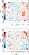 |
Fig. 5. Average of each ellipticity component in bins of the focal plane, for sources in all tomographic bins, relative to the (weighted) dispersion of ellipticities in the same bin. The weighted ellipticity dispersion per component over the bins in the focal plane are 0.287 ± 0.001 and 0.288 ± 0.001, indicating that the observed pattern is not driven by variable ellipticity dispersion across the focal plane. The figures still indicate the presence of the two-dimensional pattern reported in Figure 2 of Hildebrandt et al. (2020). |
4. Null tests
In this section, we outline the various null tests that were completed prior to the unblinding of the cosmological analysis of KiDS-Legacy; the reader interested in cosmological parameter estimates only may wish to skip to Section 5. We performed three primary tests: an analysis of the Paulin-Henriksson et al. (2008) systematics model, which quantifies the impact of PSF modelling residuals on correlation functions; an analysis of Bacon et al. (2003) statistics, which test specifically for contamination of the galaxy shape measurements by the PSF; and an analysis of B modes, which tests for a systematic signal that cannot be generated by cosmic shear.
4.1. Paulin-Henriksson et al. (2008) model
To validate the fidelity of our shape measurement catalogue, we first compute the Paulin-Henriksson et al. (2008) systematics model for KiDS-Legacy, which aims to quantify the impact of PSF modelling residuals on cosmic shear correlation functions. This systematics model, in the context of the shear two-point correlation function, reduces to the following:
![Mathematical equation: $$ \begin{aligned} \begin{aligned} \langle {\varepsilon }_{\rm obs} {\varepsilon }_{\rm obs} \rangle \simeq&\left( 1 + 2 \left[{\frac{\overline{\delta T_{\rm PSF}}}{T_{\rm gal}}}\right] \right) \left\langle {\varepsilon }_{\rm obs}^\mathrm{perfect} {\varepsilon }_{\rm obs}^\mathrm{perfect} \right\rangle \\&\quad + \, \, \left[ \,\overline{\frac{1}{T_{\rm gal}}}\,\right] ^2 \langle ({\varepsilon }_{\rm PSF} \, \delta T_{\rm PSF}) \, ({\varepsilon }_{\rm PSF} \, \delta T_{\rm PSF}) \rangle \\&\quad + \,2 \, \left[ \,\overline{\frac{1}{T_{\rm gal}}}\,\right] ^2 \langle ({\varepsilon }_{\rm PSF} \, \delta T_{\rm PSF}) \, (\delta {\varepsilon }_{\rm PSF} \, T_{\rm PSF}) \rangle \\&\quad + \, \, \left[ \,\overline{\frac{1}{T_{\rm gal}}}\,\right] ^2 \langle (\delta {\varepsilon }_{\rm PSF} \, T_{\rm PSF}) \, (\delta {\varepsilon }_{\rm PSF} \,T_{\rm PSF}) \rangle \; , \end{aligned} \end{aligned} $$](/articles/aa/full_html/2025/11/aa54908-25/aa54908-25-eq47.gif) (25)
(25)
where we only keep terms that correlate to first order. It should be noted that we use a shorthand notation in Eqs. (25), (26), and (27) as in Section 3.3 of Giblin et al. (2021), so that ⟨ab⟩ denotes ξ±. Here, εobs is the observed ellipticity of a source,  is the noiseless and unbiased measurement of source ellipticity (which we approximate as being equal to the modelled shear:
  ), and T is the R2 object size estimate.
Figure 6 shows the various contributions to the additive systematic,  , from the Paulin-Henriksson et al. (2008) systematics model. The four terms from Eq. (25), shown in various colours, cause ⟨εobsεobs⟩ to deviate from ⟨εperfectεperfect⟩. The total systematic δξ+sys:
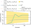 |
Fig. 6. Contributions to the additive systematic |

 (26)
(26)
is given by the summation of these four terms6 and can be compared to the yellow band which encloses 10% of the uncertainty on the cosmic shear correlation function ξ+, from the ONECOVARIANCE (Sect. 2.6). The figure presents the analysis of our sixth tomographic bin (quantitatively similar results are obtained for all other bins), and demonstrates that errors in our PSF modelling are sufficiently small (consistently less than 10% of our correlation function uncertainty) that there is no significant contamination of our two-point statistics from this source of bias. As such, we conclude that PSF modelling errors are negligible for the analysis of cosmic shear in KiDS-Legacy.
4.2. Bacon et al. (2003) statistics
We also used the method from Bacon et al. (2003) to infer the degree of PSF leakage into the two-point correlation function measurement using
 (27)
(27)
In Fig. 7, we show the value of ξ+sys in each tomographic bin autocorrelation, as a fraction of the theory prediction of the cosmic shear signal from our best-fit ξ± cosmology ( ). Results from the cross-correlation bins are quantitatively similar to the autocorrelation. As a reference, we also show 10% of the 1σ uncertainty on the cosmic shear signal as reported by the ONECOVARIANCE (Sect. 2.6). The measured fractional PSF contamination is less than the benchmark 10% of the cosmic shear correlation function uncertainty for all but five data points (out of 189 across all tomographic bin combinations). As such, we conclude that the PSF contamination of cosmic shear correlation functions is negligible in KiDS-Legacy, as expected from our PSF leakage analysis (Sect. 3.5).
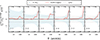 |
Fig. 7. Ratio of PSF contamination in the cosmic shear correlation function, |


4.3. B modes
Our third null test examined the significance of B-mode signals in the data vector used for cosmological analyses. This test was based on the understanding that, at the sensitivity available to stage-III cosmological imaging surveys, B-mode signals of cosmological and astrophysical origin ought to be negligible. As such, any significant detection of B modes implies a contamination of the data vector by systematic effects, which may similarly (but undiagnosably) also impact the E-modes used for cosmological inference.
We used a tomographic analysis, equivalent to that of the fiducial cosmological analysis, to derive the significance of B modes (estimated via the COSEBIs Bn) in our data vector. In the early stages of our blinded cosmological analysis, it became clear that our initial KiDS-Legacy sample failed this null test, at high significance. This led to a re-examination of the cosmological sample, which in turn led to a redefinition of the survey footprint to conservatively exclude 46.6 square-degrees with increased astrometric scatter between exposures in our lensing imaging (see Appendix E).
The B-mode signal is presented in Fig. 8. The p-values for the measured B modes across all tomographic bin combinations are 0.04 in the case of 6 Bn modes, and 0.09 in the case of 20 modes, and thus both pass our required threshold of p > 0.01 (adopted from previous work within both the KiDS and DES teams). Looking at the individual tomographic bins, only the sixth bin autocorrelation, with 6 Bn modes, has a p-value below 0.01. However, with 21 tests (one per bin combination) it is expected that one will occasionally find p < 0.01 even with correlated data drawn from the null hypothesis; indeed, this is essentially the calculation that is performed in the computation of the ‘all bins’ p-value, which passes.
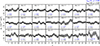 |
Fig. 8. COSEBIs B modes measured in KiDS-Legacy. Each panel is annotated with the p-value of the B-mode signals for twenty modes (black) and our fiducial 6 modes (blue). The total p-value for the full data vector, also for six and twenty modes, is annotated in the upper right corner of the figure. The B-mode signals are highly correlated across modes within a tomographic bin, so readers are cautioned against so-called ‘χ-by-eye’. |
5. Results
In this section, we present the cosmological results from KiDS-Legacy split between our fiducial results (Sect. 5.1), and variations of analysis and modelling choices (Sect. 5.2). Furthermore, we refer the reader to our companion paper (Stölzner et al. 2025) for detailed analyses of the internal consistency of KiDS-Legacy, and for analysis of the external consistency between KiDS-Legacy and datasets from DES, DESI, Pantheon+ (Brout et al. 2022), and Planck.
5.1. Fiducial constraints
The fiducial analysis of KiDS-Legacy used two statistics (En, CE) measured over  , an NLA-M intrinsic alignment model, correlated δz prior marginalisation, emulated COSMOPOWERP(k) trained on CAMB and HMCODE2020, covariances constructed with the ONECOVARIANCE and augmented with the uncertainty in the shear calibration, and sampling performed by NAUTILUS (Lange 2023) within COSMOSIS, using a Gaussian likelihood. We chose the NAUTILUS sampler due to its superior efficiency, robustness of uncertainties, and accurate evidence estimation (see e.g. Lemos et al. 2023; Dark Energy Survey and Kilo-Degree Survey Collaboration 2023). Priors for the various cosmological and nuisance parameters are given in Table 3. Correlated priors used for our redshift distribution bias parameters are given in Sect. 3.4, and for the IA model are given in Appendix B.
Fiducial prior ranges used in the analysis of KiDS-Legacy.
Constraints on S8 (α = 0.50) and Σ8 (α free).
Figure 9 presents the fiducial marginal constraints in σ8, S8, and Ωm. Marginal constraints over both S8 and Σ8 = σ8(Ωm/0.3)α (with the exponent fitted to the Ωm vs. σ8 contour) are presented in Table 4, for three estimation types: marginal mean and standard deviation, marginal mode and 1D 68% highest posterior density interval (HPDI), and maximum a posteriori (MAP) and 68% projected joint-distribution highest posterior density interval (PJ-HPD). Dark Energy Survey and Kilo-Degree Survey Collaboration (2023, Sect. 2.6) present a discussion of the benefits and detriments of each metric. We also report the χ2 of our cosmological model evaluated at the MAP, and the model probability to exceed (PTE). The MAP was evaluated using an adaptive Nelder-Mead (downhill simplex) algorithm, as described in Joachimi et al. (2021).
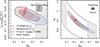 |
Fig. 9. Fiducial Ωm, S8 (left), and Ωm, σ8 (right) constraints for our fiducial two-point statistics (En and CE, orange and purple respectively), compared to the CMB results from Planck-Legacy (red). The grey contours outline the marginal distribution of our a priori volume, with (inner) 1σ and (outer) 2σ boundary levels. |
Data vectors for the fiducial En and CE are given in Fig. 10, alongside translated posterior distributions (TPDs; see Köhlinger et al. 2019), for the first application of these consistency metrics to cosmic shear datasets) drawn from the fiducial posterior computed for each statistic.
 |
Fig. 10. Data vector and TPDs for the fiducial analysis of En (upper panel) and CE (lower panel). TPDs are shown as polygons spanning the 68th (red), and 95th (orange) percentiles of the posterior models. The En signals are highly correlated across modes within a tomographic bin, so readers are cautioned against so-called ‘χ-by-eye’. The bin 2 autocorrelation signal, for example, is consistent with the best fit model (PTE = 0.09), despite the apparent divergence of the data from the model. The overall PTEs for the full tomographic dataset in each statistic are provided in Table 4. |
Our fiducial cosmological results, from COSEBIs, estimate a value of S8 = 0.813 ± 0.018, evaluated using the marginal mean and standard deviation. This is the tightest constraint made with our COSEBIs measurements, although all constraints are relatively consistent in their constraining power: the marginal mode and HPDI estimate is  , and the maximum a posteriori and PJ-HPD estimate is
  . The consistency between the measurements is a reflection of the Gaussianity of the marginal posterior, and of the N-dimensional posterior (in the case of the PJ-HPD). This is despite the necessary smoothing of the posterior distribution that is required of the HPDI computation, which is performed using a Gaussian kernel with standard deviation defined using the method of Sheather & Jones (1991). Testing of the HPDI method indicates that, for our posterior distributions in S8, the chosen smoothing kernel is unlikely to introduce additional spurious uncertainty to our cosmological parameter constraints. As such, we expect that the constraints returned from our various summarisation methods to be robust. In the following, all values and uncertainties correspond to the marginal mode and HPDI estimate, unless otherwise specified.
The above discussion about the stability of our summarisation statistics is contrasted by the observed variance between our S8 constraints from different statistics. The variance in S8 between our statistics is seemingly large, with our CE and En differing by 0.55σ. However, examination of the 2D posterior distribution in Ωm and S8 (Fig. 9) indicates that the optimal degeneracy direction for KiDS-Legacy is somewhat different than the assumed α = 0.5 parametrised by S8. This is expected, given the different scales probed by each of our statistics, and has the effect of exacerbating apparent differences between our statistics when marginalising on the S8 parameter (as translation along the degeneracy can give the false impression of internal inconsistency between final parameter constraints).
When fitting for the optimal α under the more general Σ8 = σ8(Ωm/0.3)α, we found the best fitting α is 0.58 for En and 0.60 for CE. These significant deviations from α = 0.5 can cause offsets between derived values of S8, as is seen between our CE and En constraints. Additionally, the change in degeneracy direction has a significant impact on the apparent constraining power of each of our statistics. For CE in particular, we find a significant ∼40% reduction in the relative marginal uncertainty between our S8 and Σ8 parameters. As such, we opt to preferentially present results in the Σ8 parametrisation in this manuscript, especially when quantifying the impact of analysis choices on recovered constraints. We note, however, that the different α values between the different statistics mean that Σ8 values recovered using each statistic are not directly comparable to one another.
5.2. Analysis variations
In addition to the fiducial constraints, we provide a range of additional cosmological constraints computed with various permutations of our modelling and optimisation choices. Specifically, we present: the impact of the emulation of the matter power spectrum (Sect. 5.2.1), modelling of the signal with only the Gaussian component of the covariance (Sect. 5.2.2), iterative computation of covariances (which require a pre-defined cosmology; Sect. 5.2.3), the impact of different choices of intrinsic alignment models (Sect. 5.2.4), the role of observational systematics (Sect. 5.2.5), the impact of different redshift calibrations (Sect. 5.2.6), the influence of different scale cuts (Sect. 5.2.7), and the impact of individual tomographic bins on our estimated cosmological parameters (Sect. 5.2.8).
Figure 11 presents a whisker diagram of all the various Σ8 (that is, for the optimal Ωm, σ8-degeneracy) results presented in this work. The figure includes our fiducial results in each statistic, with constraints computed using the three methods previously described in Table 4. All discussions below refer to our fiducial metric, the marginal mode and HPDI summary, unless stated otherwise. Additionally, we have annotated the figure with a measure of the difference between our various results, computed using the metric (Σ8fid − Σ8var)/σΣ8var. Differences are computed between the Σ8 values of each setup and the fiducial. We also annotate the fiducial constraints with their Hellinger distance (see e.g. Appendix G.1 of Heymans et al. 2021) to the constraints from the public, fiducial Planck-Legacy analysis (Planck Collaboration VI 2020). Finally, we present a similar figure for S8 in Appendix G, and tables of all constraints are presented in Appendix H.
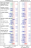 |
Fig. 11. Whisker diagram of Σ8 cosmological results presented in this work. The best-fitting α used for each statistic is annotated on the x-axis. Each panel shows the compilation of results for one of our two-point statistics, as annotated. In each panel, we show the fiducial constraints in the relevant statistic with coloured points (colour-coded by the statistic), and highlight the fiducial marginal HPDI with a band of the equivalent colour. We also highlight the marginal HPDI in Σ8 from Planck-Legacy (shaded red). All variations to the analysis are annotated, with the difference relative to the fiducial result quantified using the metric (Σ8fid − Σ8var)/σΣ8var (listed in blue). The Hellinger tension between the fiducial analyses and Planck is annotated in red. |
5.2.1. Modelling P(k) with CAMB
We tested the impact of the COSMOPOWER emulator by re-running our fiducial analysis directly with CAMB and comparing the cosmological constraints between these runs in Fig. 11. We found that, for all statistics, the CAMB posteriors were consistent with those estimated with the emulated power spectrum, showing maximal changes in the marginal value of Σ8 of 0.03σ. We consider this level of change to be consistent with chain-to-chain variations, and therefore negligible.
5.2.2. Gaussian covariance
We tested the impact of our covariance modelling on the recovered value of Σ8 in Fig. 11, by performing the fiducial measurement with only the Gaussian component of the covariance activated in the ONECOVARIANCE code. We found a reduction in the uncertainty on Σ8 of between 12% (CE) and 19% (En), and no change in the value of Σ8 with respect to the fiducial (ΔΣ8 = 0.02σ). This is an indication that, while shape noise is still sufficient to shroud information on non-linear scales, KiDS-Legacy has a non-negligible contribution to its constraining power from these non-Gaussian scales.
5.2.3. Iterative covariance
The covariance used in our cosmological inference modelling assumes a fixed cosmology. If this fixed cosmology differs from the best-fit cosmology preferred by the dataset, this can add a source of inconsistency in our fiducial results. Therefore, as with previous KiDS analyses (see e.g. van Uitert et al. 2018), we verified the fidelity of our cosmological inference by recomputing the fiducial sample covariances at the maximum a posteriori cosmology for each chain, and rerun our cosmological inference. This iterative evaluation of the covariance and cosmological parameters do not need to converge after a single iteration, and so we ran this process for many (≲10) iterations. We found that the cosmological constraints (and constraining power) converged after two iterations, even for our most complex model choices. This is in good agreement with previous investigations into the impact of varying cosmological parameters on covariances in the context of stage-III surveys (Reischke et al. 2017; Kodwani et al. 2019).
5.2.4. Intrinsic alignment modelling
We tested the cosmological parameter constraints recovered when modelling intrinsic alignments with our four different models. The resulting cosmological parameters are presented in Fig. 11.
First, we see that the impact of changing our IA models on the marginal constraints of S8 and Σ8 are mild. For our CE statistic, we found maximal differences of 0.17σ across all model variations. Also, En values are more sensitive to our chosen IA model, showing maximal differences of 0.54σ (for the NLA and NLA-k models and Σ8). Second, we see that changing the IA model has a minor impact on the constraining power of our survey, with systematic changes in constraining power being most evident for the NLA-z model: we see a consistent reduction in constraining power (compared to the fiducial NLA-M model) of 12 − 13% for Σ8 across all statistics. For our NLA and NLA-k models, the reduction in constraining power compared to the fiducial is slightly smaller, at ∼5%. This reduced constraining power (despite the fact that e.g. the NLA model has fewer parameters) is attributed to the informative prior applied in our NLA-M model (see Sect. 2.4.4 and Appendix B). Finally, we also note mild changes to our recovered goodness-of-fit under the various IA models. In all cases, the χ2 of the modified IA model is consistent with the fiducial (changes in PTE at the orderof 1 − 5%).
The stability of our cosmological constraints under variation of the IA modelling provides confidence that any possible misspecification of the IA model is unlikely to introduce bias in our cosmological parameter constraints. Furthermore, we can compare the implied amplitude of IA under each of our models by examining the AIA, total values (see Eqs. (8), (10), (12)). Figure 12 shows the value of AIA, total inferred from our En analysis, as a function of redshift. All statistics show quantitatively similar behaviour. In Appendix G, we present the posterior distributions in all parameters (Figs. G.2 and G.3) for each IA model.
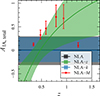 |
Fig. 12. Constraints on the total intrinsic alignment amplitude from the various intrinsic alignment models, per tomographic bin (where appropriate), computed using the En posteriors. Bands and error bars represent the 1σ posterior constraint on each model. Our NLA-M model (red) is shown per tomographic bin, with the point positioned at the mean photo-z of the bin. |
For our NLA and NLA-k models, there is no explicit dependence on tomographic bin number (or, more accurately, redshift), and thus the IA amplitude is necessarily constant across the redshift axis for these models. Both of these models are consistent with IA amplitudes of zero. A change in IA amplitude with redshift is nominally expected, though, as the combination of Malmquist bias and the mass-scaling of IA amplitudes combine to increase the effective measured IA with increasing redshift, thereby motivating our NLA-z and NLA-M models.
For our fiducial NLA-M model, the IA do change with tomographic bin, due to their varying fraction of passive/red galaxies and their typical mass (blue galaxies have zero IA in this model). In our analysis, the alignment amplitudes initially climb through bins one to five, but rapidly drop in bin six where there are very few galaxies with an early-type SED (see Appendix B and Table B.1)7. As such, the NLA-M model represents a functional form that is not accessible to any of our other models. It is therefore interesting to note the similarity between the inferred values of AIA, total in our NLA-z and NLA-M models. Both show the expected increase in alignment amplitudes with increasing redshift, although the NLA-z model is at slightly lower amplitudes overall. We attribute this difference to the sixth tomographic bin: as the NLA-z model requires that all bins follow the same (monotonic) trend, any reduction in AIA, total between the fifth and sixth tomographic bins will require a compensatory reduction in alignment amplitude across all bins.
5.2.5. Impact of observational and systematic nuisance parameters
To demonstrate the impact of the various nuisance parameters and the relative importance of marginalisation over various priors, we ran a posterior analysis with our intrinsic alignment model uncertainty (σIA) and redshift and shear calibration uncertainty (σz, σm) nuisance parameters set to zero. The associated parameters to these uncertainties were fixed to the centre of their fiducial prior. We repeated the posterior calculation using only the remaining (cosmological and physical) parameters. Figure 11 shows these results. We found that the posterior constraints on Σ8 in the absence of marginalisation over these observational and systematic nuisance parameters are tighter by 10% (20%) for our En (CE) measurements, and are shifted with respect to the fiducial by 0.28σ (0.14σ). This suggests that KiDS-Legacy is statistics-limited.
5.2.6. Alternative redshift distribution calibration
We analysed the changes in parameter constraints found under different redshift calibration scenarios. In particular, we demonstrate the constraints found when we switch off shape-measurement weighting of the calibration sample, and when we switch off prior volume weighting of the calibration sample. In both cases, we found that the cosmological constraints are consistent with our fiducial constraints, showing a mild increase of ΔΣ8 ≤ 0.17σ. This is, to some degree, expected: if our redshift distribution estimation changed appreciably when modifying our calibration method, this would also be reflected in our estimated bias parameters δz. As such, this test is particularly relevant for demonstrating possible sensitivity to source galaxies that reside outside the redshift baseline of our SKiLLS simulations. The lack of significant change in our cosmological parameters under changing the redshift calibration methodology suggests that our analysis is not strongly influenced by sources outside the redshift limits of SKiLLS.
Conversely, we also show in Fig. 11 the result of calibrating our redshift distributions using simulations from MICE2. These are the simulations that were used for KiDS-1000 N(z) calibration, but differ here in that we applied our KiDS-Legacy calibration methodology to these simulations. Wright et al. (2025) discuss the accuracy of the redshift distribution bias parameters estimated from MICE2, in particular possible biases due to the MICE2 redshift limits of 0.1 ≲ z ≲ 1.4. As our bin six N(z) (in particular) extends beyond this upper limit, it is expected that our redshift distribution bias parameters there will be inaccurate. Therefore, we include them here predominantly as a demonstration of the effect of switching from MICE2 to SKiLLS. The maximum difference in the mean redshifts between our fiducial (effective) N(z) and that from MICE2 is Δμz, eff = 0.016, in bin 3. However, the difference found is coherent between bins 3 − 6, which is therefore expected to cause a shift in S8. As seen in Fig. 11, our analysis using N(z) calibrated with the MICE2 simulations increases the central value of our Σ8 constraints, by up to 1.25σ (for En). We consider these results inferior to the fiducial redshift calibration, though, given the considerably less realistic simulations (compared to SKiLLS), and the smaller redshift baseline that truncates the sixth bin to half of its supposed width.
In addition to our SOM calibrated redshift distributions, we also show results using our redshift distributions calibrated to cross-correlation measurements (Wright et al. 2025). Our cosmological constraints from this analysis are essentially unchanged in their central value for both En and CE, showing a 0.01σ shift in the central value of Σ8 (computed with the fiducial α for each statistic). However, the results have lower constraining power, given the larger uncertainty in (particularly) the sixth tomographic bin: uncertainties in the optimal projection of Σ8 are 23% (29%) larger for our CC N(z)/δ(z) marginalisation than in the fiducial case for En (CE). Nonetheless, the strong agreement between the estimates made with our CC and SOM N(z) provides confidence that redshift distribution biases in KiDS-Legacy are under control.
5.2.7. Scale cuts
In KiDS-1000, Asgari et al. (2021) presented cosmological constraints using a range of angular scales from  . Subsequent investigation by Dark Energy Survey and Kilo-Degree Survey Collaboration (2023), however, found that an optimal treatment of baryonic systematic effect mitigation (for En/Bn) was achieved using
  . For KiDS-1000 (Asgari et al. 2021), this resulted in a shift in the marginal parameter constraints of S8 at the level of 0.8σ. Reanalysis of KiDS-1000 by Li et al. (2023a), with improved shape measurement and calibration from Li et al. (2023c), showed a reduced sensitivity to the choice of scale cut, seeing a shift of 0.3σ. We also tested the influence of changing our scale cuts, shown in the marginal projection of Ωm, S8 in Fig. 13, finding that including smaller scales results in a slight (0.1σ) decrease in the marginal value of Σ8 and S8. We also saw a slight change in the preferred value of our baryonic feedback parameter (see Fig. 13) where there is a reduction in posterior probability mass at negligible feedback amplitudes (i.e. log10(TAGN/K)≈7.3, consistent with dark-matter only) when adding in smaller scale information. However, this must be interpreted with caution, as both posteriors are formally prior dominated in this parameter. This extra data is expected to be sensitive to baryon feedback, but it is difficult to distinguish from a simple change in the noise realisation. In either case, though, it is clear that the additional scales have at most a minor impact on our cosmological constraints.
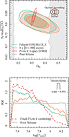 |
Fig. 13. Comparison of the marginal constraints on Ωm and S8 (top) and log10(TAGN/K) (bottom) when using a wider range of scales ( |

We note that the expanded scale cut has a non-negligible effect on the significance of our B mode null test, causing it to once again fail our p > 0.01 requirement. A full reanalysis of the additional astrometric selections required to reach non-significance in our null test with this expanded scale cut has not been explored here, and so the accuracy of the constraints with these expanded scales is not guaranteed. Nonetheless, the stability of the cosmological constraints in the presence of both baryonic feedback contamination and possible systematics contamination is encouraging.
5.2.8. Removing tomographic redshift bins
In previous analyses of KiDS, the removal of individual tomographic bins (including all cross-correlations) introduced changes in marginal cosmological constraints of up to 1.8σ in Σ8.(see e.g. Asgari et al. 2021). We performed the same test here, and show the results in Fig. 11. We found that our cosmological results are more robust to the removal of individual tomographic bins than previous work from KiDS: we observe a maximal difference in Σ8 when removing individual bins of 0.24σ for En, 0.17σ for CE. We attribute this decreased sensitivity at least partly to the reduction in relative importance of each tomographic bin (as signal is shared more evenly between the bins using our approximately equal-number tomography, and sixth bin). Furthermore, in our companion paper (Stölzner et al. 2025), we performed a series of internal consistency tests aimed at specifically estimating the constraints from different combinations of tomographic bins, finding that they were all consistent with each other, unlike KiDS-1000. As such, this represents a considerable improvement in internal consistency for KiDS that we attribute to the enhanced redshift calibration samples and methodology, as well as with the general improvements in data quality seen in Legacy compared to previous KiDS data releases.
6. Discussion
The results from KiDS-Legacy are consistent with the results of Planck Legacy, with a marginal Σ8 consistency of 0.73σ for En and 1.01σ for CE. The constraints from KiDS-Legacy are also of comparable constraining power to those from Planck when projected into Σ8, with Planck having a marginal uncertainty of ±0.015 compared to Legacy’s 0.016.
Compared to previous cosmological constraints from KiDS, Legacy represents a decrease in the marginal tension with Planck (computed using the Hellinger distance) of 2.2σ, compared to previous work from Li et al. (2023a), who utilised methods and modelling choices that most resemble those used in Legacy. Such a difference in marginal constraints from individual KiDS analyses was deemed acceptable prior to unblinding (indeed, such a judgement call was required prior to unblinding), however was nonetheless surprising to the authors. This prompted an investigation into the underlying drivers of the change in cosmological constraints between the two samples.
A complete description of the investigation into the consistency between KiDS-1000 and KiDS-Legacy is provided in Appendix I. In summary, we found that improvements to our redshift distribution estimation and calibration methodology are responsible for approximately two thirds (1.32σ) of the reduction in marginal tension with Planck, as reported by KiDS-1000 and Legacy. An additional reduction is attributable to a reduction in statistical noise from the sources outside the KiDS-1000 footprint. These results are shown graphically in Fig. I.1.
We also explored the consistency between our new Legacy cosmological parameters with recent results from the literature. Figure 14 presents the En cosmological constraints from Legacy in the context of two recent stage-III cosmic shear analyses: DES-Y3 hybrid-pipeline results from Dark Energy Survey and Kilo-Degree Survey Collaboration (2023), and 2PCF measurements from HSC-Y3 (Li et al. 2023b). DES-Y3 is a largely independent analysis (there is a small on-sky overlap), which is also most consistent with Legacy: differences between marginal cosmological parameter constraints are 0.75σ in Σ8 and 0.41σ in S8. Comparisons to the joint analysis of DESY3 and KiDS-1000, or to HSC, are both more covariate (due to area overlap) and show larger differences (1.5σ and 1.8σ in Σ8 respectively), but are otherwise consistent. Overall, we found good consistency between all samples presented here, and with Planck. To this end, there is no evidence of significant tension in S8 (or in the more constraining Σ8) from KiDS-Legacy. Furthermore, the consistency that we found between KiDS-Legacy and other low-redshift cosmological probes motivates the joint analysis of cosmological parameters with these surveys, which can be found in our companion paper (Stölzner et al. 2025). Lastly, as mentioned before, we do not include ξ± into our fiducial analysis. However, the constraints and resulting consistency metrics are very similar and is discussed in Appendix F.
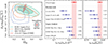 |
Fig. 14. Comparison between KiDS-Legacy En cosmological constraints and recent stage-III cosmic shear survey results from the literature. We show the 2D posteriors for each analysis Ωm, S8 (left) as well as the marginal projections in Σ8 (α = 0.58, middle), and S8 (right). The 1D marginal ‘whisker’ plots are annotated as previously: circular points represent marginal mode and HPD intervals, while diamonds represent maximum a posteriori points and their associated PJ-HPD. Values are all calculated directly from the chains released by each analysis/survey, and in all cases except Legacy we take the MAP directly from the chain. We see that all surveys presented here are consistent with both KiDS-Legacy (black annotations) and Planck (red annotations) using our fiducial consistency metric of |ΔX|≤2.6σ (where X is either Σ8 or S8), as estimated using the Hellinger tension between marginal mode summaries. |
We performed an analysis of the effective constraining power provided by KiDS-Legacy over the matter power spectrum P(k) and the amplitude of baryon feedback. Figure 15 shows our constraint over P(k) from the fiducial En, estimated by sampling the full posterior of KiDS-Legacy and generating posterior predictive distributions for P(k) using CAMB and HMCODE2020. We show the P(k) constraint normalised to the mean of all posterior samples, with a 0.1σ region shaded around this central reference. This allows us to directly compare our P(k) constraint to the distribution of P(k) returned by two power spectrum emulators, BACCO (Aricò et al. 2021) and EUCLIDEMULATOR2 (Euclid Collaboration: Knabenhans et al. 2021), also evaluated at the same posterior samples. We note, though, that these emulators have a reduced range of validity compared to our fiducial priors, particularly in ns. Nonetheless, we see that the differences between the emulated power spectra and those returned by CAMB are within the 0.1σ credible interval of our posterior constraint on P(k), demonstrating that differences between the various P(k) models (evaluated at the same cosmological and nuisance parameters) are consistently less than 10% of our constraining power, and are thus unlikely to be a significant source of bias in our analysis. With increased constraining power (from e.g. stage-IV surveys), however, the uncertainty in our modelling of P(k) will become a significant fraction of the finaluncertainty.
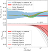 |
Fig. 15. Upper panel: Estimate of the systematic uncertainty in our modelling of the matter power spectrum using CAMB and HMCODE2020, compared to two P(k) emulators BACCO (green) and EUCLIDEMULATOR2 (orange). The figure shows the ratio between the power spectrum from CAMB and HMCODE2020 to those returned by each emulator, evaluated at 10 000 representative samples from the fiducial En/Bn posterior with a tenth of a standard-deviation. Lower panel: Constraints on baryonic feedback suppression from KiDS-Legacy. The marginal HPDI of feedback amplitudes from our fiducial En/Bn is shown in red, relative to a range of hydrodynamical models of baryonic feedback suppression from FLAMINGO(Schaye et al. 2023). |
We also explored the importance of baryon feedback modelling on our cosmological constraints, by examining the posterior on our feedback amplitude parameter log10(TAGN/K) in the context of our P(k) constraints. We found that the contribution to the power spectrum from our inferred feedback amplitude is negligible for scales k ≲ 0.2 h/Mpc. Above this scale our posterior constraint on the feedback model introduces a 1 − 10% suppression in power (compared to the dark-matter only case), and is consistent with the fiducial baryon feedback model from FLAMINGO at all scales. Above approximately k = 1 h/Mpc, our marginal posterior on P(k) excludes the more extreme FLAMINGO feedback models. Our MAP estimate of log10(TAGN/K) is at the lower boundary limit of the prior, indicating that our best-fitting model prefers negligible baryon feedback amplitudes. Our marginal constraint over log10(TAGN/K) is unconstrained (see Fig. 13), but is nonetheless skewed towards the MAP value.
Finally, given the agreement between our cosmological constraints and those from Planck, we investigated the inferred amplitude of baryon feedback with cosmological parameters fixed to those reported by Planck. This has the effect of placing a strong informative prior that the cosmological model is as described by Planck, and used cosmic shear to marginalise effectively over only observational systematic effects (IA, δz, and baryon feedback). Our posterior constraints over all systematic parameters are essentially unchanged with respect to the fiducial, with the only small change of note being that our baryon feedback posterior skewed slightly more strongly towards the lower prior boundary of log10(TAGN/K) = 7.3, while the MAP remains at the boundary (see Fig. 13). In the fiducial case our marginal posterior on log10(TAGN/K) was unconstrained (using the metric of Asgari et al. 2021, see their Appendix A), however with the informative Planck prior we were able to place an upper limit constraint of log10(TAGN/K)≤7.71 (8.01) at one-sided 68% (95%) confidence. As such, we argue that there is little evidence in KiDS-Legacy for significant amplitudes of baryon feedback, even when placing strong informative priors on cosmological parameters.
7. Summary
We present a cosmological analysis of the completed Kilo-Degree Survey (KiDS). Utilising data from KiDS Data Release 5 (Wright et al. 2024), we constructed our cosmic shear source sample from 1347 square degrees of optical and near-infrared imaging, containing deeper imaging, new astrometric and photometric calibrations, and cleaner masking of spurious sources and artefacts. Our improved data was then coupled with a greatly expanded spectroscopic calibration dataset named ‘KiDZ’ (consisting of 2.4 − 5.0 times the spectra as used in the analysis of KiDS-1000), along with an updated redshift distribution calibration methodology (‘gold-weight’; see Wright et al. 2025). This allowed us to calibrate sources at higher redshifts than those in any previous KiDS analysis. We defined six tomographic bins, spanning photometric redshifts between 0.1 < zB ≤ 2.0, and calibrated the source redshift distributions with a precision up to six times higher than previously possible. We calibrated the source shapes using multi-band image simulations (Li et al. 2023c), finding that the KiDS-Legacy sample has the lowest systematic contamination (by e.g. PSF leakage) of any KiDS dataset to date. As per standard practices in the field, our cosmological analysis was performed fully blind.
Our fiducial cosmological parameter constraints were estimated with COSEBIs (En), utilising conservative θ ∈ [2.0, 300.0] arcmin scales and a new physically-motivated intrinsic alignment (IA) model. Our fiducial En measurement constrains  , which is in full agreement (Hellinger distance of 0.76σ) with the marginal prediction
  from the Planck Legacy cosmic microwave background experiment. Our fiducial measurement represents a ∼15% improvement in constraining power over the previous results from KiDS. However, we also found a significant change in optimal degeneracy between σ8 and Ωm, with Σ8 ≡ σ8(Ωm/0.3)α and α = 0.58 being preferred by our En measurement. We found
  , which is a ∼32% improvement in optimal constraining power compared to previous KiDS analyses. In this projection, the corresponding Hellinger distance to Planck is 0.73σ. We further computed the cosmological parameters using band power spectra (CE) and found full agreement with our fiducial COSEBIs. We performed a number of analysis variations, with our cosmological parameter constraints shown to be consistent across all modelling choices, statistics, tomographic bins, and summary statistics. Our companion paper (Stölzner et al. 2025) presents a full suite of internal and external consistency tests, finding the KiDS-Legacy dataset to be the most internally robust sample produced by KiDS to date.
We tested for systematic bias with respect to previous results from KiDS, finding that most of the differences in parameter constraints can be attributed to improved redshift distribution estimation and calibration, as well as new survey area and improved image reduction. We leveraged our consistency with Planck to estimate the preferred baryon feedback amplitude of KiDS-Legacy, allowing us to place an upper limit on log10TAGN ≤ 7.71 (8.01) at 68% (95%) confidence. As such, the results from KiDS-Legacy paint a harmonious picture of cosmology at the end of stage-III, with full agreement between the cosmological parameters estimated by both low- and high-redshift probes of cosmic structure.
We use TREECORR version 4.2.3, with binslop = 1.5.
Other binning options are also explored in the literature, which can alleviate some of the issues with the top-hat response function at the expense of broadening the range of ℓ-values that contribute to each bin (see e.g. Becker et al. 2016).
The terms in Eq. (25) are related to the often-used and so-called ‘ρ’-statistics, as recommended by Rowe (2010) and Jarvis et al. (2016). In contrast to the total systematic term δξ+sys (Eq. 26), the systematic requirements on the ‘ρ-statistics, relative to the statistical noise on the measured cosmic shear signal, are unspecified. We therefore chose not to explore the ‘ρ’-statistics directly.
This may be a (suboptimal) feature of our SED based classification, which is unable to reliably identify the precursor sources of modern pressure-supported systems using uncertain SED models, especially at high-z.
Four of our parameters were kept fixed to fiducial values in our power spectra: the curvature contribution to the total energy density (ΩK) was fixed to zero, the sum of the neutrino masses (∑mν) was fixed to its minimum standard value, and the equation-of-state parameters of dark energy (w0, wa), were fixed at the values for a cosmological constant. See Table 3.
Acknowledgments
The authors would like to sincerely thank Matthias Bartelmann, who has acted as the external blinding coordinator for every blinded analysis performed by KiDS in the last 10+ years. AHW and HHi are supported by the Deutsches Zentrum für Luft- und Raumfahrt (DLR), made possible by the Bundesministerium für Wirtschaft und Klimaschutz, under project 50QE2305, and acknowledge funding from the German Science Foundation DFG, via the Collaborative Research Center SFB1491 “Cosmic Interacting Matters – From Source to Signal”. BS, CH, & ZY acknowledge support from the Max Planck Society and the Alexander von Humboldt Foundation in the framework of the Max Planck-Humboldt Research Award endowed by the Federal Ministry of Education and Research. MA is supported by the UK Science and Technology Facilities Council (STFC) under grant number ST/Y002652/1 and the Royal Society under grant numbers RGSR2222268 and ICAR1231094. MB & PJ are supported by the Polish National Science Center through grant no. 2020/38/E/ST9/00395. MB is also supported by grant no. 2020/39/B/ST9/03494. BG acknowledges support from the UKRI Stephen Hawking Fellowship (grant reference EP/Y017137/1). CH also acknowledges support from the UK Science and Technology Facilities Council (STFC) under grant ST/V000594/1. HHi, CM, RR, & AD are supported by an ERC Consolidator Grant (No. 770935). HHi is also supported by a DFG Heisenberg grant (Hi 1495/5-1). HHo & MY acknowledge support from the European Research Council (ERC) under the European Union’s Horizon 2020 research and innovation program with Grant agreement No. 101053992. BJ acknowledges support by the ERC-selected UKRI Frontier Research Grant EP/Y03015X/1 and by STFC Consolidated Grant ST/V000780/1. KK acknowledges support from the Royal Society and Imperial College. SSL is receiving funding from the programme “Netzwerke 2021”, an initiative of the Ministry of Culture and Science of the State of North-Rhine Westphalia. MvWK acknowledges the support by the UKSA and STFC (grant no. ST/X001075/1). PB acknowledges financial support from the Canadian Space Agency (Grant No. 23EXPROSS1) and the Waterloo Centre for Astrophysics. CG is funded by the MICINN project PID2022-141079NB-C32. JHD acknowledges support from an STFC Ernest Rutherford Fellowship (project reference ST/S004858/1) SJ acknowledges the Ramón y Cajal Fellowship (RYC2022-036431-I) from the Spanish Ministry of Science and the Dennis Sciama Fellowship at the University of Portsmouth. LL is supported by the Austrian Science Fund (FWF) [ESP 357-N]. AL acknowledges support from the research project grant ‘Understanding the Dynamic Universe’ funded by the Knut and Alice Wallenberg Foundation under Dnr KAW 2018.0067. CM acknowledges support from the Beecroft Trust, and the Spanish Ministry of Science under the grant number PID2021-128338NB-I00. LM acknowledges support from STFC grant ST/N000919/1. LMo acknowledges the financial contribution from the grant PRIN-MUR 2022 20227RNLY3 “The concordance cosmological model: stress-tests with galaxy clusters” supported by Next Generation EU and from the grant ASI n. 2024-10-HH.0 ‘Attività scientifiche per la missione Euclid – fase E’. NRN acknowledges financial support from the National Science Foundation of China, Research Fund for Excellent International Scholars (grant n. 12150710511), and from the research grant from China Manned Space Project n. CMS-CSST-2021-A01. LP acknowledges support from the DLR grant 50QE2002. MR acknowledges financial support from the INAF grant 2022. TT acknowledges funding from the Swiss National Science Foundation under the Ambizione project PZ00P2_193352. YZ acknowledges the studentship from the UK Science and Technology Facilities Council (STFC). Based on observations made with ESO Telescopes at the La Silla Paranal Observatory under programme IDs 179.A-2004, 177.A-3016, 177.A-3017, 177.A-3018, 298.A-5015. This work was performed in part at Aspen Center for Physics, which is supported by National Science Foundation grant PHY-1607611. Author Contributions: All authors contributed to the development and writing of this paper. The authorship list is given in three groups: the lead authors (AHW, BS), followed by two alphabetical groups. The first alphabetical group includes those who are key contributors to both the scientific analysis and the data products of this manuscript and release. The second group covers those who have either made a significant contribution to the preparation of data products or to the scientific analyses of KiDS-Legacy.
References
- Abdalla, E., Abellán, G. F., Aboubrahim, A., et al. 2022, J. High Energy Astrophys., 34, 49 [NASA ADS] [CrossRef] [Google Scholar]
- Ahumada, R., Allende Prieto, C., Almeida, A., et al. 2020, ApJS, 249, 3 [NASA ADS] [CrossRef] [Google Scholar]
- Amon, A., & Efstathiou, G. 2022, MNRAS, 516, 5355 [CrossRef] [Google Scholar]
- Amon, A., Gruen, D., Troxel, M. A., et al. 2022, Phys. Rev. D, 105, 023514 [NASA ADS] [CrossRef] [Google Scholar]
- Aricò, G., Angulo, R. E., Hernández-Monteagudo, C., et al. 2020, MNRAS, 495, 4800 [Google Scholar]
- Aricò, G., Angulo, R. E., Contreras, S., et al. 2021, MNRAS, 506, 4070 [CrossRef] [Google Scholar]
- Asgari, M., & Schneider, P. 2015, A&A, 578, A50 [NASA ADS] [CrossRef] [EDP Sciences] [Google Scholar]
- Asgari, M., Schneider, P., & Simon, P. 2012, A&A, 542, A122 [NASA ADS] [CrossRef] [EDP Sciences] [Google Scholar]
- Asgari, M., Tröster, T., Heymans, C., et al. 2020, A&A, 634, A127 [NASA ADS] [CrossRef] [EDP Sciences] [Google Scholar]
- Asgari, M., Lin, C.-A., Joachimi, B., et al. 2021, A&A, 645, A104 [NASA ADS] [CrossRef] [EDP Sciences] [Google Scholar]
- Bacon, D. J., Massey, R. J., Refregier, A. R., & Ellis, R. S. 2003, MNRAS, 344, 673 [NASA ADS] [CrossRef] [Google Scholar]
- Bartelmann, M., & Schneider, P. 2001, Phys. Rep., 340, 291 [Google Scholar]
- Becker, M. R., Troxel, M. A., MacCrann, N., et al. 2016, Phys. Rev. D, 94, 022002 [NASA ADS] [CrossRef] [Google Scholar]
- Benítez, N. 2000, ApJ, 536, 571 [Google Scholar]
- Bertin, E., & Arnouts, S. 1996, A&AS, 117, 393 [NASA ADS] [CrossRef] [EDP Sciences] [Google Scholar]
- Blake, C., Brough, S., Couch, W., et al. 2008, Astron. Geophys., 49, 5.19 [Google Scholar]
- Blake, C., Amon, A., Childress, M., et al. 2016, MNRAS, 462, 4240 [NASA ADS] [CrossRef] [Google Scholar]
- Blazek, J. A., MacCrann, N., Troxel, M. A., & Fang, X. 2019, Phys. Rev. D, 100, 103506 [NASA ADS] [CrossRef] [Google Scholar]
- Bridle, S., & King, L. 2007, New J. Phys., 9, 444 [Google Scholar]
- Brout, D., Scolnic, D., Popovic, B., et al. 2022, ApJ, 938, 110 [NASA ADS] [CrossRef] [Google Scholar]
- Broxterman, J. C., & Kuijken, K. 2024, A&A, 692, A201 [NASA ADS] [CrossRef] [EDP Sciences] [Google Scholar]
- Capaccioli, M., Mancini, D., & Sedmak, G. 2005, The Messenger, 120, 10 [NASA ADS] [Google Scholar]
- Carretero, J., Castander, F. J., Gaztañaga, E., Crocce, M., & Fosalba, P. 2015, MNRAS, 447, 646 [NASA ADS] [CrossRef] [Google Scholar]
- Catelan, P., Kamionkowski, M., & Blandford, R. D. 2001, MNRAS, 320, L7 [NASA ADS] [CrossRef] [Google Scholar]
- Crittenden, R. G., Natarajan, P., Pen, U.-L., & Theuns, T. 2001, ApJ, 559, 552 [CrossRef] [Google Scholar]
- Crocce, M., Castander, F. J., Gaztañaga, E., Fosalba, P., & Carretero, J. 2015, MNRAS, 453, 1513 [NASA ADS] [CrossRef] [Google Scholar]
- Dalal, R., Li, X., Nicola, A., et al. 2023, Phys. Rev. D, 108, 123519 [CrossRef] [Google Scholar]
- Dark Energy Survey and Kilo-Degree Survey Collaboration (Abbott, T. M. C., et al.) 2023, Open J. Astrophys., 6, 36 [NASA ADS] [Google Scholar]
- DESI Collaboration (Adame, A. G., et al.) 2024, AJ, 168, 58 [NASA ADS] [CrossRef] [Google Scholar]
- Driver, S. P., Hill, D. T., Kelvin, L. S., et al. 2011, MNRAS, 413, 971 [Google Scholar]
- Driver, S. P., Bellstedt, S., Robotham, A. S. G., et al. 2022, MNRAS, 513, 439 [NASA ADS] [CrossRef] [Google Scholar]
- Edge, A., Sutherland, W., Kuijken, K., et al. 2013, The Messenger, 154, 32 [NASA ADS] [Google Scholar]
- Euclid Collaboration (Knabenhans, M., et al.) 2021, MNRAS, 505, 2840 [NASA ADS] [CrossRef] [Google Scholar]
- Euclid Collaboration (Mellier, Y., et al.) 2025, A&A, 697, A1 [Google Scholar]
- Fenech Conti, I., Herbonnet, R., Hoekstra, H., et al. 2017, MNRAS, 467, 1627 [NASA ADS] [Google Scholar]
- Fortuna, M. C., Hoekstra, H., Johnston, H., et al. 2021a, A&A, 654, A76 [NASA ADS] [CrossRef] [EDP Sciences] [Google Scholar]
- Fortuna, M. C., Hoekstra, H., Joachimi, B., et al. 2021b, MNRAS, 501, 2983 [NASA ADS] [CrossRef] [Google Scholar]
- Fortuna, M. C., Dvornik, A., Hoekstra, H., et al. 2025, A&A, 694, A322 [NASA ADS] [CrossRef] [EDP Sciences] [Google Scholar]
- Fosalba, P., Crocce, M., Gaztañaga, E., & Castander, F. J. 2015a, MNRAS, 448, 2987 [NASA ADS] [CrossRef] [Google Scholar]
- Fosalba, P., Gaztañaga, E., Castander, F. J., & Crocce, M. 2015b, MNRAS, 447, 1319 [NASA ADS] [CrossRef] [Google Scholar]
- Gaia Collaboration (Brown, A. G. A., et al.) 2018, A&A, 616, A1 [NASA ADS] [CrossRef] [EDP Sciences] [Google Scholar]
- Ge, F., Millea, M., Camphuis, E., et al. 2025, Phys. Rev. D, 111, 083534 [Google Scholar]
- Georgiou, C., Chisari, N. E., Bilicki, M., et al. 2025, A&A, 699, A252 [NASA ADS] [CrossRef] [EDP Sciences] [Google Scholar]
- Giblin, B., Heymans, C., Asgari, M., et al. 2021, A&A, 645, A105 [NASA ADS] [CrossRef] [EDP Sciences] [Google Scholar]
- Gong, Y., Liu, X., Cao, Y., et al. 2019, ApJ, 883, 203 [NASA ADS] [CrossRef] [Google Scholar]
- Grandis, S., Aricò, G., Schneider, A., & Linke, L. 2024, MNRAS, 528, 4379 [NASA ADS] [CrossRef] [Google Scholar]
- Guzzo, L., Scodeggio, M., Garilli, B., et al. 2014, A&A, 566, A108 [NASA ADS] [CrossRef] [EDP Sciences] [Google Scholar]
- Heydenreich, S., Schneider, P., Hildebrandt, H., et al. 2020, A&A, 634, A104 [NASA ADS] [CrossRef] [EDP Sciences] [Google Scholar]
- Heymans, C., Brown, M. L., Barden, M., et al. 2005, MNRAS, 361, 160 [Google Scholar]
- Heymans, C., White, M., Heavens, A., Vale, C., & van Waerbeke, L. 2006, MNRAS, 371, 750 [Google Scholar]
- Heymans, C., Grocutt, E., Heavens, A., et al. 2013, MNRAS, 432, 2433 [Google Scholar]
- Heymans, C., Tröster, T., Asgari, M., et al. 2021, A&A, 646, A140 [NASA ADS] [CrossRef] [EDP Sciences] [Google Scholar]
- Hikage, C., Oguri, M., Hamana, T., et al. 2019, PASJ, 71, 43 [Google Scholar]
- Hilbert, S., Hartlap, J., White, S. D. M., & Schneider, P. 2009, A&A, 499, 31 [NASA ADS] [CrossRef] [EDP Sciences] [Google Scholar]
- Hildebrandt, H., Köhlinger, F., van den Busch, J. L., et al. 2020, A&A, 633, A69 [NASA ADS] [CrossRef] [EDP Sciences] [Google Scholar]
- Hildebrandt, H., van den Busch, J. L., Wright, A. H., et al. 2021, A&A, 647, A124 [EDP Sciences] [Google Scholar]
- Hirata, C. M., & Seljak, U. 2004, Phys. Rev. D, 70, 063526 [Google Scholar]
- Hoekstra, H., Yee, H. K. C., & Gladders, M. D. 2002, ApJ, 577, 595 [Google Scholar]
- Hoffmann, K., Bel, J., Gaztañaga, E., et al. 2015, MNRAS, 447, 1724 [NASA ADS] [CrossRef] [Google Scholar]
- Howlett, C., Lewis, A., Hall, A., & Challinor, A. 2012, JCAP, 04, 027 [Google Scholar]
- Ivezić, Ž., Kahn, S. M., Tyson, J. A., et al. 2019, ApJ, 873, 111 [Google Scholar]
- Jarvis, M., Bernstein, G., & Jain, B. 2004, MNRAS, 352, 338 [Google Scholar]
- Jarvis, M., Sheldon, E., Zuntz, J., et al. 2016, MNRAS, 460, 2245 [Google Scholar]
- Jee, M. J., Tyson, J. A., Hilbert, S., et al. 2016, ApJ, 824, 77 [Google Scholar]
- Joachimi, B., Schneider, P., & Eifler, T. 2008, A&A, 477, 43 [NASA ADS] [CrossRef] [EDP Sciences] [Google Scholar]
- Joachimi, B., Mandelbaum, R., Abdalla, F. B., & Bridle, S. L. 2011, A&A, 527, A26 [NASA ADS] [CrossRef] [EDP Sciences] [Google Scholar]
- Joachimi, B., Lin, C. A., Asgari, M., et al. 2021, A&A, 646, A129 [NASA ADS] [CrossRef] [EDP Sciences] [Google Scholar]
- Johnston, H., Georgiou, C., Joachimi, B., et al. 2019, A&A, 624, A30 [NASA ADS] [CrossRef] [EDP Sciences] [Google Scholar]
- Johnston, H., Wright, A. H., Joachimi, B., et al. 2021, A&A, 648, A98 [NASA ADS] [CrossRef] [EDP Sciences] [Google Scholar]
- Kaiser, N. 1992, ApJ, 388, 272 [Google Scholar]
- Kilbinger, M., Fu, L., Heymans, C., et al. 2013, MNRAS, 430, 2200 [Google Scholar]
- Kilbinger, M., Heymans, C., Asgari, M., et al. 2017, MNRAS, 472, 2126 [Google Scholar]
- Knabenhans, M., Brinckmann, T., Stadel, J., Schneider, A., & Teyssier, R. 2023, MNRAS, 518, 1859 [Google Scholar]
- Kodwani, D., Alonso, D., & Ferreira, P. 2019, Open J. Astrophys., 2, 3 [NASA ADS] [CrossRef] [Google Scholar]
- Köhlinger, F., Joachimi, B., Asgari, M., et al. 2019, MNRAS, 484, 3126 [NASA ADS] [Google Scholar]
- Kohonen, T. 1982, Biological Cybernetics, 43, 59 [CrossRef] [Google Scholar]
- Kuijken, K. 2011, The Messenger, 146, 8 [NASA ADS] [Google Scholar]
- Kuijken, K., Heymans, C., Hildebrandt, H., et al. 2015, MNRAS, 454, 3500 [Google Scholar]
- Kuijken, K., Heymans, C., Dvornik, A., et al. 2019, A&A, 625, A2 [NASA ADS] [CrossRef] [EDP Sciences] [Google Scholar]
- Lamman, C., Tsaprazi, E., Shi, J., et al. 2024, Open J. Astrophys., 7, 14 [NASA ADS] [CrossRef] [Google Scholar]
- Lange, J. U. 2023, MNRAS, 525, 3181 [NASA ADS] [CrossRef] [Google Scholar]
- Le Fèvre, O., Vettolani, G., Garilli, B., et al. 2005, A&A, 439, 845 [Google Scholar]
- Lemos, P., Weaverdyck, N., Rollins, R. P., et al. 2023, MNRAS, 521, 1184 [NASA ADS] [CrossRef] [Google Scholar]
- Leonard, C. D., Ferreira, T., Fang, X., et al. 2023, Open J. Astrophys., 6, 8 [CrossRef] [Google Scholar]
- Lewis, A., Challinor, A., & Lasenby, A. 2000, ApJ, 538, 473 [Google Scholar]
- Li, S.-S., Hoekstra, H., Kuijken, K., et al. 2023a, A&A, 679, A133 [NASA ADS] [CrossRef] [EDP Sciences] [Google Scholar]
- Li, X., Zhang, T., Sugiyama, S., et al. 2023b, Phys. Rev. D, 108, 123518 [CrossRef] [Google Scholar]
- Li, S.-S., Kuijken, K., Hoekstra, H., et al. 2023c, A&A, 670, A100 [NASA ADS] [CrossRef] [EDP Sciences] [Google Scholar]
- LoVerde, M., & Afshordi, N. 2008, Phys. Rev. D, 78, 123506 [NASA ADS] [CrossRef] [Google Scholar]
- Alonso, D., Sanchez, J., Slosar, A., & LSST Dark Energy Science Collaboration 2019, MNRAS, 484, 4127 [NASA ADS] [CrossRef] [Google Scholar]
- MacCrann, N., Becker, M. R., McCullough, J., et al. 2022, MNRAS, 509, 3371 [Google Scholar]
- Mandelbaum, R., Seljak, U., Kauffmann, G., Hirata, C. M., & Brinkmann, J. 2006, MNRAS, 368, 715 [NASA ADS] [CrossRef] [Google Scholar]
- Mandelbaum, R., Blake, C., Bridle, S., et al. 2011, MNRAS, 410, 844 [Google Scholar]
- McCarthy, I. G., Schaye, J., Bird, S., & Le Brun, A. M. C. 2017, MNRAS, 465, 2936 [Google Scholar]
- McCullough, J., Amon, A., Legnani, E., et al. 2024, ArXiv e-prints [arXiv:2410.22272] [Google Scholar]
- Mead, A. 2015, Astrophysics Source Code Library [record ascl:1508.001] [Google Scholar]
- Mead, A. J., Brieden, S., Tröster, T., & Heymans, C. 2021, MNRAS, 502, 1401 [Google Scholar]
- Miller, L., Kitching, T. D., Heymans, C., Heavens, A. F., & van Waerbeke, L. 2007, MNRAS, 382, 315 [Google Scholar]
- Miller, L., Heymans, C., Kitching, T. D., et al. 2013, MNRAS, 429, 2858 [Google Scholar]
- Newman, J. A., Cooper, M. C., Davis, M., et al. 2013, ApJS, 208, 5 [Google Scholar]
- Oehl, V., & Tröster, T. 2024, ArXiv e-prints [arXiv:2407.08718] [Google Scholar]
- Paulin-Henriksson, S., Amara, A., Voigt, L., Refregier, A., & Bridle, S. L. 2008, A&A, 484, 67 [NASA ADS] [CrossRef] [EDP Sciences] [Google Scholar]
- Pen, U.-L., Van Waerbeke, L., & Mellier, Y. 2002, ApJ, 567, 31 [Google Scholar]
- Piras, D., Joachimi, B., Schäfer, B. M., et al. 2018, MNRAS, 474, 1165 [Google Scholar]
- Planck Collaboration VI. 2020, A&A, 641, A6 [NASA ADS] [CrossRef] [EDP Sciences] [Google Scholar]
- Preston, C., Amon, A., & Efstathiou, G. 2023, MNRAS, 525, 5554 [NASA ADS] [CrossRef] [Google Scholar]
- Qu, F. J., Sherwin, B. D., Madhavacheril, M. S., et al. 2024, ApJ, 962, 112 [NASA ADS] [CrossRef] [Google Scholar]
- Reischke, R., Kiessling, A., & Schäfer, B. M. 2017, MNRAS, 465, 4016 [CrossRef] [Google Scholar]
- Reischke, R., Unruh, S., Asgari, M., et al. 2025, A&A, 699, A124 [NASA ADS] [CrossRef] [EDP Sciences] [Google Scholar]
- Rowe, B. 2010, MNRAS, 404, 350 [NASA ADS] [Google Scholar]
- Salcido, J., McCarthy, I. G., Kwan, J., Upadhye, A., & Font, A. S. 2023, MNRAS, 523, 2247 [NASA ADS] [CrossRef] [Google Scholar]
- Samuroff, S., Blazek, J., Troxel, M. A., et al. 2019, MNRAS, 489, 5453 [NASA ADS] [CrossRef] [Google Scholar]
- Samuroff, S., Mandelbaum, R., Blazek, J., et al. 2023, MNRAS, 524, 2195 [Google Scholar]
- Schaller, M., Schaye, J., Kugel, R., Broxterman, J. C., & van Daalen, M. P. 2025, MNRAS, 539, 1337 [Google Scholar]
- Schaye, J., Kugel, R., Schaller, M., et al. 2023, MNRAS, 526, 4978 [NASA ADS] [CrossRef] [Google Scholar]
- Schneider, M. D., & Bridle, S. 2010, MNRAS, 402, 2127 [Google Scholar]
- Schneider, A., & Teyssier, R. 2015, JCAP, 2015, 049 [Google Scholar]
- Schneider, P., van Waerbeke, L., Jain, B., & Kruse, G. 1998, MNRAS, 296, 873 [NASA ADS] [CrossRef] [Google Scholar]
- Schneider, P., van Waerbeke, L., & Mellier, Y. 2002, A&A, 389, 729 [NASA ADS] [CrossRef] [EDP Sciences] [Google Scholar]
- Schneider, P., Eifler, T., & Krause, E. 2010, A&A, 520, A116 [NASA ADS] [CrossRef] [EDP Sciences] [Google Scholar]
- Schneider, A., Giri, S. K., Amodeo, S., & Refregier, A. 2022, MNRAS, 514, 3802 [NASA ADS] [CrossRef] [Google Scholar]
- Scoville, N., Aussel, H., Brusa, M., et al. 2007, ApJS, 172, 1 [Google Scholar]
- Secco, L. F., Samuroff, S., Krause, E., et al. 2022, Phys. Rev. D, 105, 023515 [NASA ADS] [CrossRef] [Google Scholar]
- Semboloni, E., Hoekstra, H., Schaye, J., van Daalen, M. P., & McCarthy, I. G. 2011, MNRAS, 417, 2020 [Google Scholar]
- Sheather, S. J., & Jones, M. C. 1991, J. Roy. Stat. Soc. Ser. B (Methodol.), 53, 683 [Google Scholar]
- Shuntov, M., McCracken, H. J., Gavazzi, R., et al. 2022, A&A, 664, A61 [NASA ADS] [CrossRef] [EDP Sciences] [Google Scholar]
- Skrutskie, M. F., Cutri, R. M., Stiening, R., et al. 2006, AJ, 131, 1163 [NASA ADS] [CrossRef] [Google Scholar]
- Spergel, D., Gehrels, N., Baltay, C., et al. 2015, ArXiv e-prints [arXiv:1503.03757] [Google Scholar]
- Spurio Mancini, A., Piras, D., Alsing, J., Joachimi, B., & Hobson, M. P. 2022, MNRAS, 511, 1771 [NASA ADS] [CrossRef] [Google Scholar]
- Stölzner, B., Wright, A. H., Asgari, M., et al. 2025, A&A, 702, A169 [NASA ADS] [CrossRef] [EDP Sciences] [Google Scholar]
- Takahashi, R., Sato, M., Nishimichi, T., Taruya, A., & Oguri, M. 2012, ApJ, 761, 152 [Google Scholar]
- Tessore, N., Loureiro, A., Joachimi, B., von Wietersheim-Kramsta, M., & Jeffrey, N. 2023, Open J. Astrophys., 6, 11 [NASA ADS] [CrossRef] [Google Scholar]
- Tonegawa, M., Okumura, T., & Hayashi, M. 2025, PASJ, 77, 389 [Google Scholar]
- Tröster, T., Asgari, M., Blake, C., et al. 2021, A&A, 649, A88 [NASA ADS] [CrossRef] [EDP Sciences] [Google Scholar]
- van den Busch, J. L., Hildebrandt, H., Wright, A. H., et al. 2020, A&A, 642, A200 [NASA ADS] [CrossRef] [EDP Sciences] [Google Scholar]
- van Uitert, E., Cacciato, M., Hoekstra, H., & Herbonnet, R. 2015, A&A, 579, A26 [NASA ADS] [CrossRef] [EDP Sciences] [Google Scholar]
- van Uitert, E., Cacciato, M., Hoekstra, H., et al. 2016, MNRAS, 459, 3251 [Google Scholar]
- van Uitert, E., Joachimi, B., Joudaki, S., et al. 2018, MNRAS, 476, 4662 [NASA ADS] [CrossRef] [Google Scholar]
- von Wietersheim-Kramsta, M., Lin, K., Tessore, N., et al. 2025, A&A, 694, A223 [NASA ADS] [CrossRef] [EDP Sciences] [Google Scholar]
- Wright, A. H., Hildebrandt, H., van den Busch, J. L., et al. 2020, A&A, 640, L14 [NASA ADS] [CrossRef] [EDP Sciences] [Google Scholar]
- Wright, A. H., Kuijken, K., Hildebrandt, H., et al. 2024, A&A, 686, A170 [NASA ADS] [CrossRef] [EDP Sciences] [Google Scholar]
- Wright, A. H., Hildebrandt, H., van den Busch, J. L., et al. 2025, A&A, submitted [arXiv:2503.19440] [Google Scholar]
- Yan, Z., Wright, A. H., Elisa Chisari, N., et al. 2025, A&A, 694, A259 [NASA ADS] [CrossRef] [EDP Sciences] [Google Scholar]
- Yoon, M., & Jee, M. J. 2021, ApJ, 908, 13 [NASA ADS] [CrossRef] [Google Scholar]
- Yoon, M., Jee, M. J., Tyson, J. A., et al. 2019, ApJ, 870, 111 [Google Scholar]
- Zuntz, J., Paterno, M., Jennings, E., et al. 2015, Astron. Comput., 12, 45 [NASA ADS] [CrossRef] [Google Scholar]
Appendix A: Emulating matter power spectra with COSMOPOWER
The most computationally expensive section of our modelling pipeline is the prediction of the matter power spectra with CAMB. Fortunately, we can circumvent this time-consuming computation through the use of artificial neural network emulators, which act to provide a direct non-linear mapping between input cosmological parameters and the corresponding output power spectrum. Such an emulator can be created with relative ease using the COSMOPOWER framework of Spurio Mancini et al. (2022). The original COSMOPOWER emulator was trained to reproduce the linear matter power spectrum, Pm, lin(k), and the perturbations caused by non-linear evolution, Pm, nl(k)/Pm, lin(k), given a set of relevant input parameters. We updated this process to emulate residuals log10[P(k)/Pref(k)] between logarithmic power spectra (for both linear and non-linear spectra) and a single reference power spectrum instead. The reference spectrum was chosen to be near the centre of our sampling/prior volume, which is defined by the ranges of the various parameters in Table 3. These ranges subsequently also define the range of validity of our emulator.
Construction of the emulator requires a large sample of training and testing power-spectra, which were generated by CAMB, over the seven-dimensional8 volume that we wish to sample. For this purpose, we generated 450 000 training and 50 000 testing spectra, produced by a Latin hypercube sampling over our volume.
The consistency between our emulated spectra and the target spectra returned by CAMB and HMCODE2020 is validated in the publicly available emulator repository on GitHub9, through computation of the distribution of absolute fractional residuals between the target and estimated spectra for all 50 000 testing samples. We found that our updated method of emulation produces a more uniform error distribution than the original emulation method from Spurio Mancini et al. (2022), across the wide range of scales that we emulate (k ∈ [10−5, 20] h/Mpc), and generally reduces the maximum error over all scales. Our emulator exhibits a maximal error below 0.1% for 68% of our test samples, in both the linear and non-linear power spectra.
Appendix B: Galaxy sample properties for intrinsic alignment modelling
For our fiducial galaxy-type and mass-dependent intrinsic alignment (IA) model, we need to measure the average host halo mass Mh and the red galaxy fraction fr in each tomographic bin. These, and relevant intermediate properties, are summarised in Table B.1. We note that, where appropriate, we computed averages as the means over logarithmic quantities as these propagate straightforwardly to the averages of derived quantities in power-law relations. Moreover, all averages were weighted by the shear measurement weight and redshift estimation gold weight.
Early-type galaxy sample properties for the mass-dependent intrinsic alignment model per tomographic bin.
To determine fr, we used the output of the photometric redshift estimation from the template-fitting code BPZ (Benítez 2000). BPZ employs a set of six model templates, ordered in terms of star formation activity, and interpolates linearly between adjacent template to determine a best-fitting spectral energy distribution. The BPZ output TB encodes the best-fit templates and their admixture in steps of 0.1. We chose TB < 1.9 to define early-type galaxies, encompassing all galaxies with some contribution of an elliptical galaxy spectrum (template no. 1). We validated that, at least on a matched sample between the KiDS and GAMA (Driver et al. 2011) surveys (i.e. for relatively bright and low-redshift galaxies), this TB cut is capable of isolating the red sequence.
We found that in the first five tomographic bins fr fluctuates around 0.2, broadly in line with expectations for a flux-limited sample. The sixth bin contains a negligible fraction of early-type galaxies, a feature that we also see in our simulated sixth bin from SKiLLS. The statistical error on fr is very small. We repeated the measurement varying TB by ±0.1 and obtained changes in fr of less than 0.02. Therefore, we decided to consider fr as fixed in the IA model.
To compute halo masses, we made use of the r-band luminosities derived as part of the KiDS Data Release 5 (Wright et al. 2024). van Uitert et al. (2015) measured effective halo masses for SDSS (LOWZ and CMASS) early-type galaxies via weak lensing, as a function of luminosity and redshift. We used their reported halo mass results and galaxy properties to construct the following linear relation
![Mathematical equation: $$ \begin{aligned} \log _{10} M_{\rm h}^{(i)} [h^{-1} M_\odot ]&= \gamma \left( \frac{1}{1+\langle z \rangle ^{(i)}} - \frac{1}{1+z_{\rm piv}} \right)\\ \nonumber&\;\; + \delta \, \log _{10} \left( \frac{\langle L_r\rangle ^{(i)} }{ L_0 } \right) + \Delta M\;, \end{aligned} $$](/articles/aa/full_html/2025/11/aa54908-25/aa54908-25-eq83.gif) (B.1)
(B.1)
where we chose zpiv = 0.3417, such that the parameters γ and ΔM are uncorrelated to a good approximation. An additional parameter δ describes the dependence on the average luminosity ⟨Lr⟩, normalised by the reference luminosity L0 = 1011(h/0.7)−2 L⊙. van Uitert et al. (2015) showed that the luminosity dependence evolves only mildly with redshift, so that we determine δ as the inverse variance-weighted average scaling over the four samples they considered. Thus, we obtained γ = 1.25 ± 0.33, δ = 1.42 ± 0.16, and ΔM = 13.56 ± 0.02. In line with expectations, both the average luminosity and halo mass increase monotonically by more than an order of magnitude from the first to the sixth tomographic bin (see Table B.1).
Statistical uncertainties on the halo mass are propagated via Monte Carlo sampling from the fit and measurement uncertainties. The standard deviation of log10Mh is approximately 0.2 in the first tomographic bin, driven by the extrapolation of Eq. (B.1) to fainter samples, and of order 0.1 in the remaining bins, where a reduced error due to luminosities more compatible with the range fitted by van Uitert et al. (2015) is gradually traded off with larger uncertainty because of extrapolation to higher redshifts. Halo mass estimates are strongly correlated (correlation coefficient greater than 0.9) between tomographic bins due to the extrapolation from the luminosity and redshift ranges considered by van Uitert et al. (2015). Therefore, we propagated the uncertainty in halo masses into our IA model by assuming a multivariate Gaussian prior with standard deviation of 0.2 in log10Mh for all bins and the correlation matrix as obtained from the Monte Carlo error propagation.
Throughout the construction of our astrophysics-informed galaxy IA model, we have not distinguished between central and satellite galaxies, although their alignment mechanisms are believed to be different (Schneider & Bridle 2010). The NLA model assumes a fixed relation between linear and non-linear scales where centrals and satellites tend to dominate IA signals, respectively, although our scale-dependent IA model tests whether the data prefers a different ratio on average over the whole survey. However, the satellite fraction in our early-type galaxy sample is unknown, yet almost certainly evolves with halo mass and redshift (see e.g. Shuntov et al. 2022). For a given mass and redshift, early-type satellite fractions are typically twice as large as those of late types (Mandelbaum et al. 2006), so that the impact of potential IA signals of blue satellites is less of a concern.
Moreover, the satellite fractions in most galaxy samples used in direct IA constraints are also unknown. Fortuna et al. (2025) estimated a satellite fraction of 30 % and possibly higher (see also van Uitert et al. 2016) in a subset of the GAMA-KiDS sample and subsequently excluded it from their fit. Johnston et al. (2019) studied alignments amongst and between centrals and satellites. They tentatively found a steeper slope of the red satellite IA signal on small transverse scales. The mass scaling of the IA amplitude in red satellites is qualitatively similar to that of centrals (Fortuna et al. 2021b).
In summary, neither cosmic shear surveys nor direct measurements to calibrate IA currently provide sufficient information to treat the IA signals of satellites and their associated trends separately. We are forced to treat satellite effects as part of an effective small-scale IA model, with any discrepancies in the combined dependencies on scale and galaxy sample properties expected to be comfortably absorbed in the still wide priors. Once surveys reach the statistical power to significantly constrain IA models beyond an overall amplitude, calibration measurements of IA will need to be (re-)analysed separately for central and satellite populations. Halo models (Fortuna et al. 2021b) will be a natural choice to accurately represent different IA mechanisms and scalings on large and small scales.
Appendix C: Band-powers derivation
To arrive at the correct response functions for our band-powers, we first write  as a function of ξ±(θ), in the same manner as for the COSEBIs in Eq. (16),
![Mathematical equation: $$ \begin{aligned} {\mathcal{C} }_{\mathrm{E/B},l} = \frac{\pi }{{\mathcal{N} }_l}\; \int _0^\infty \mathrm{d} \theta \, \theta \; T(\theta ) \left[ g_+^l(\theta )\;\xi _+(\theta )\; \pm g_-^l(\theta )\;\xi _-(\theta )\right]\;, \end{aligned} $$](/articles/aa/full_html/2025/11/aa54908-25/aa54908-25-eq85.gif) (C.1)
(C.1)
where g±l(θ) are the band-power filter functions for bin l and T(θ) is a function that limits the range of θ-scales that contribute to the integral. If ξ± is known for all scales then T(θ) = 1 everywhere. We now write g±l(θ) in terms of the idealised response function,
 (C.2)
(C.2)
If Sl(ℓ) is a top-hat then,
![Mathematical equation: $$ \begin{aligned} g_+^l(\theta )&= \frac{1}{\theta ^2} \left[\theta \ell _{\mathrm{up},l}\; \mathrm{J}_1(\theta \ell _{\mathrm{up},l}) - \theta \ell _{\mathrm{lo},l}\; \mathrm{J}_1(\theta \ell _{\mathrm{lo},l}) \right] \;, \\ \nonumber g_-^l(\theta )&= \frac{1}{\theta ^2} \left[\mathcal{G}_-(\theta \ell _{\mathrm{up},l}) - \mathcal{G}_-(\theta \ell _{\mathrm{lo},l}) \right]\;, \end{aligned} $$](/articles/aa/full_html/2025/11/aa54908-25/aa54908-25-eq87.gif) (C.3)
(C.3)
with,
 (C.4)
(C.4)
Inserting for ξ± from Eq. (15) into Eq. (C.1) we arrive at,
![Mathematical equation: $$ \begin{aligned} \mathcal{C}_{\mathrm{E},l}^{(ij)}&= \frac{1}{2 \mathcal{N}_l} \int _0^\infty \mathrm{d} \ell \; \ell \left[ W^l_{\rm EE}(\ell )\; C^{(ij)}_{{\varepsilon } {\varepsilon }, \mathrm E}(\ell ) + W^l_{\rm EB}(\ell )\; C^{(ij)}_{{\varepsilon } {\varepsilon }, \mathrm B}(\ell ) \right]\; , \\ \nonumber \mathcal{C}_{\mathrm{B},l}^{(ij)}&= \frac{1}{2 \mathcal{N}_l} \int _0^\infty \mathrm{d} \ell \; \ell \left[ W^l_{\rm BE}(\ell )\; C^{(ij)}_{{\varepsilon } {\varepsilon }, \mathrm E}(\ell ) + W^l_{\rm BB}(\ell )\; C^{(ij)}_{{\varepsilon } {\varepsilon }, \mathrm B}(\ell ) \right]\;, \end{aligned} $$](/articles/aa/full_html/2025/11/aa54908-25/aa54908-25-eq89.gif) (C.5)
(C.5)
where the weight functions are,
![Mathematical equation: $$ \begin{aligned} \begin{aligned} W^l_{\rm EE}(\ell )&= \!\! \int _0^\infty \!\! \mathrm{d} \theta \, \theta \; T(\theta ) \left[ \mathrm{J}_0(\ell \theta )\; g_+^l(\theta ) + \mathrm{J}_4(\ell \theta )\; g_-^l(\theta ) \right]\;, \\ W^l_{\rm EB}(\ell )&= \!\! \int _0^\infty \!\! \mathrm{d} \theta \, \theta \; T(\theta ) \left[\mathrm{J}_0(\ell \theta )\; g_+^l(\theta ) - \mathrm{J}_4(\ell \theta )\; g_-^l(\theta ) \right]\;, \end{aligned} \end{aligned} $$](/articles/aa/full_html/2025/11/aa54908-25/aa54908-25-eq90.gif) (C.6)
(C.6)
with WEEl(ℓ) = WBBl(ℓ) and WEBl(ℓ) = WBEl(ℓ). Since ξ± are measured between θmin and θmax, T(θ) has to be defined such that no information beyond this range is included. To avoid ringing, we apodise T(θ) with a Hahn window and smooth its transitions to zero:
![Mathematical equation: $$ \begin{aligned} T(\theta ) = \left\{ \begin{aligned} 0\,;&\; x < x_{\rm lo} - \frac{\Delta _x}{2} \\ \cos ^2 \left[\frac{\pi }{2} \frac{x- (x_{\rm lo}+\Delta _x/2)}{\Delta _x} \right]\,;&\; x_{\rm lo} -\frac{\Delta _x}{2} \le x < x_{\rm lo} +\frac{\Delta _x}{2} \\ 1 \,;&\; x_{\rm lo} +\frac{\Delta _x}{2} \le x < x_{\rm up} -\frac{\Delta _x}{2} \\ \cos ^2 \left[\frac{\pi }{2} \frac{x-(x_{\rm up} - \Delta _x/2)}{\Delta _x} \right]\,;&\; x_{\rm up} -\frac{\Delta _x}{2} \le x < x_{\rm up} +\frac{\Delta _x}{2}\\ 0 \,;&\; x \ge x_{\rm up} +\frac{\Delta _x}{2}\;. \end{aligned} \right. \end{aligned} $$](/articles/aa/full_html/2025/11/aa54908-25/aa54908-25-eq91.gif) (C.7)
(C.7)
Here x = log(θ), Δx is the log-width of the apodisation, xlo − Δx/2 = log(θmin) and xup + Δx/2 = log(θmax). We require Δx > log(θup/θlo), and in practice have used Δx = 0.5 for all KiDS-Legacy CE, B analyses. We note, also, that this apodisation method is different to how we applied the apodisation for KiDS-1000 analysis, where we instead had xlo = log(θmin) and xup = log(θmax). This change was made as it was deemed more intuitive/appropriate that the band power windows be contained primarily within the requested ℓ ranges after apodisation, rather than before.
Appendix D: KiDS-Legacy variable depth mocks and covariance validation
Our analysis used an analytical covariance matrix, as summarised in Sect. 2.6. Here, we describe the mocks which were used to validate the covariance matrix (see Reischke et al. 2025) in more detail.
The log-normal simulations are based on GLASS10 (Generator for Large-Scale Structure, Tessore et al. 2023) with a detailed description given in von Wietersheim-Kramsta et al. (2025) as well as Section 8.1 in Reischke et al. (2025). The resulting density field realisations, in concentric shells, were subsequently integrated along the line-of-sight weighted by the weak lensing kernel, Eq. (2), to create a total of 4224 realisations of the shear field.
For each realisation, galaxies were sampled, factoring in systematic effects such as the survey footprint and variable depth (as caused by seeing, sky transparency fluctuations, and differences in the number of overlapping pointings) using SALMO11 (Speedy Acquisition for Lensing and Matter Observables, Joachimi et al. 2021). The inclusion of a sixth tomographic bin in KiDS-Legacy incorporates more faint galaxies in the sample, enhancing the overall magnitude of variable depth and boosting the lensing signal relative to the noise. Although previous analyses suggested that depth variability effects on the signal in KiDS-1000 remain below the noise threshold (Heydenreich et al. 2020), this might not be the case for KiDS-Legacy.
To model variable depth, we rely on organised randoms (ORs, introduced in Johnston et al. 2021; Yan et al. 2025). ORs use SOMs to generate random samples that reflect the spatial variability caused by a high-dimensional systematic space. The ORs provide Tiaogeng (TG) weights, wTG, (see Yan et al. 2025, for a detailed explanation), quantifying the spatial variability of the selection function of the galaxy sample as a function of position on the sky. The ORs robustly trace the variations in depth for KiDS-Legacy. Yan et al. (2025) demonstrated that the TG weights are uncorrelated with r-band magnitude, photometric redshift, and underlying cosmological density variations. In contrast, they are highly correlated with the magnitude limit of the survey in the r-band, which is used for both source extraction and shape measurement.
Figure D.1 shows the TG weights for a single field in our KiDS-Legacy-like mock, as a function of position on the simulated sky. Additionally, Fig. D.2 shows the corresponding local source density of sources as a function of TG weights, colour-scaled for the different source bins. The horizontal dashed lines depict the effective homogeneous number density. Solid lines are linear fits to the measured effective number density in ten equi-populated bins of the TG weights. This linear interpolation allows for an effective evaluation of neff at each pixel.
 |
Fig. D.1. Cartesian spatial map (corresponding Nside = 1024, showing a local flat projection of the healpix map) of the TG weights, wTG, throughout a single field of our KiDS-Legacy-like mock catalogue. Larger TG weights correspond to a higher local source density. |
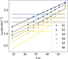 |
Fig. D.2. Dependence of the galaxy density, neff, on TG weights, wTG in the KiDS-Legacy-like mock catalogue. The data points represent the mean neff of ten equi-populated bins in wTG. The solid line shows the linear fit to the aforementioned data points of their respective tomographic bin, labelled S1-S6. The dashed horizontal lines show the mean values of neff calculated from the galaxy samples with variable depth per tomographic bin, while the dashed horizontal lines show the values of neff for the respective galaxy samples without any spatial variations in the observational depth. |
The local density variations seen here also affect the redshift distributions. This issue is addressed by reapplying the photometric redshift calibration using SOMs (see Wright et al. 2025, for details) to each tomographic bin and each of the ten TG weight bins. The resulting redshift distribution then enters the shear maps via the weak lensing kernel.
On each simulation, we measured the shear two-point correlation functions as indicated in Sect. 2.5, from which the sample covariance could be estimated directly. These mocks were then compared to the ONECOVARIANCE code. The results are presented in Reischke et al. (2025) with 10 percent agreement for the variances, very similar to what was found in previous analysis (Joachimi et al. 2021). In particular, we found that the limiting factor in the covariance modelling is not the effect of variable depth but rather the survey geometry on large scales. All these effects, however, do not significantly affect the cosmological results presented in this paper.
Appendix E: B-mode analysis
During the initial phases of the blinded KiDS-Legacy analysis, our B-mode null-test analyses (see Sect. 4.3) failed our required significance threshold (p ≥ 0.01). This led to a dedicated effort to investigate the possible causes of the B-mode signal in the dataset, starting with the highest level data products and systematically working our way back through the data production and analysis pipelines, to identify the root cause of the B-mode signal.
As KiDS-1000 did not show significant B modes (specifically, as analysed by Li et al. 2023a using the same shape-measurement code and analysis choices, such as scale cuts), the initial test in our investigation was to determine whether the observed B-mode significance in KiDS-Legacy was owing to a decrease in covariance (specifically shot noise) caused by the increased area of KiDS-Legacy over KiDS-1000. We therefore started by analysing the KiDS-Legacy B-mode significance in the same footprint as KiDS-1000, finding that the KiDS-Legacy data in this footprint still exceeded the B-mode significance requirement.
Subsequent investigation of the B-mode origin focussed on PSF contamination (via Paulin-Henriksson statistics; see Sect. 4), one- and two-dimensional c-terms, covariance construction, and shape measurement biases (as a function of, for example, galaxy morphology and position on-sky). Each of these tests was performed locally (per square degree tile), in the detector plane (i.e. coadding all sources in the frame of the focal plane), with spatial jackknife subsets of the full survey, and globally (e.g. at the data vector level, and looking for population-level trends). Each of these investigations failed to illuminate the origin of the B-mode signal. Finally, we investigated the lowest-level possible cause of the anomalous B-mode signal: systematic failures in the astrometric solution used in the THELI calibration (with Gaia) of r-band images. The global astrometric accuracy of KiDS-Legacy is presented in Wright et al. (2024), where we demonstrated the accuracy of the THELI (constructed with a Gaia reference) and ASTRO-WISE (constructed with a SDSS and 2MASS reference) catalogues both globally (see their Figures 10, 11, C1, and C2) and as a function of right ascension and declination (RA and Dec; see their Figures 8 and 9), compared to SDSS, 2MASS, and Gaia. In our new investigation, we explored the astrometric accuracy in finer detail (i.e. higher on-sky resolution) and using the individual astrometric solutions of THELI exposures and ASTRO-WISE co-adds.
We computed two test statistics for investigation of the B-mode signal. The first test statistic is sensitive to the astrometric consistency between THELI co-added images, which are used for source detection, and ASTRO-WISE co-added images, which are used for photometric measurements (and therefore impacts photometric redshift estimation, which is used for tomographic binning). This metric (δrint) measured the systematic difference between the centroid of all targets extracted from these images. This was achieved by matching all sources (within 2″) extracted from ASTRO-WISE and THELI co-added r-band images. With these matches, we computed the radial separation r between each source’s centroid in the two images and then calculated the median of these separations in 1 × 1 arcminute on-sky bins. The 2D map of median separations was then assigned back to each source.
Our second test statistic was computed between individual exposures of the THELIr-band images, which are used for shape measurement. This metric (δrexp) measures the systematic difference between the centroids of targets extracted from individual THELI exposures, which are point-like and have high S/N. This was achieved by matching sources extracted from ASTRO-WISE (used here purely as a static reference) and the individual THELI exposures (within 2″). For the ASTRO-WISE static reference, we applied selections on SOURCE EXTRACTOR (Bertin & Arnouts 1996) output variables
 (E.1)
(E.1)
and
 (E.2)
(E.2)
to select point-like high-S/N sources. Settings used in the extraction of sources are provided in Table 4 of Wright et al. (2024). For the sources extracted from the individual THELI exposures, we performed the same point source selection (Eq. E.1) and a modified S/N criteria, to account for the reduced depth of the individual exposures compared to the co-add:
 (E.3)
(E.3)
With these matches, we then computed the radial separation rij between all exposures in {i, j ∈ [1, 5] | i ≠ j}, computed the maximum of these separations in 2 × 2 arcminute on-sky bins, and smoothed these maps with a 1 arcminute Gaussian kernel. We then combined these individual 15 i ↔ j maps into a final single map, by selecting again the maximum separation per on-sky bin. This resulting map was then once-again smoothed using a 1 arcminute Gaussian kernel.
These maps provided us with two test statistics that could be used as an additional mask for the survey, given specific thresholds in the statistic values. The first metric is relevant for possible failures in photometry: if the astrometric solution between ASTRO-WISE and THELI differs, then the apertures extracted from THELI imaging will be incorrectly placed on the ASTRO-WISE images. The second metric is relevant for possible failures in shape measurement: the shape measurement algorithm lensfit, which is used in KiDS, assumes perfect astrometric alignment of exposures within the THELIr-band imaging. As such, any residual astrometric misalignment will manifest as an erroneously estimated shape, and coherent misalignments may manifest as an E- or B-mode cosmic-shear signal.
For our first statistic, the degree of inconsistency between the imaging that can lead to systematic errors in photometry is relatively benign: our photometric measurement code GAAP has a minimum aperture size of  , driven largely by the fact that our imaging has seeing that is consistently larger than
  (see e.g. Figure 7 of Wright et al. 2024). Systematic errors in aperture centroids at the level of the FWHM and larger will lead to significant flux to be lost from the target aperture (assuming a point-like source), and thus may pose a problem for our photometry. However, there are two additional relevant considerations. Firstly, in our cosmological analyses, all sources that are used must be resolved and thus (in some direction) larger than the PSF FWHM. Secondly, even if significant flux is missed, if the ASTRO-WISE imaging are all well aligned to each other, then the flux will be consistently missed in all bands, thereby keeping the source SED largely consistent. As such, we expect the effect to be rarely relevant, and (when it is relevant) only to have a minor impact on photometric redshifts. Nonetheless, we chose to mask all areas of the survey where our first statistic exceeds the minimum PSF FWHM: that is, where
  . This corresponds to approximately 0.7 deg2 of removed data over the full KiDS-Legacy footprint.
For our astrometric statistic, there is much less intuition available regarding the level of astrometric error that may be problematic for our analysis. As such, we chose to investigate (while remaining fully blinded; outcomes of the various tests were very similar for all blinds) the impact of various masks (defined by thresholds in δrexp) on our null test results, and on our cosmological inference. Figure E.1 shows the results of this investigation. On the x-axis of each panel in the figure, we show the threshold in our astrometric metric δrexp that was used to define a mask. This mask was then applied to the full KiDS-Legacy cosmic shear source sample, and the end-to-end cosmological analysis pipeline was run (including N(z) estimates, shape recalibration, two-point statistics, covariances, and cosmological chains). For each threshold, we were therefore able to report the change in sample size (bottom panel of Fig. E.1; similar to the change in area), the change in the B-mode null test p-value (middle panel), and the change in the inferred marginal value of Σ8 (top panel).
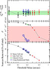 |
Fig. E.1. Summary of our blinded B-mode investigation where we measure the COSEBIs En/Bn cosmic shear statistics, masking survey area where our astrometric metric, δrexp, exceeds a series of threshold values (shown on the x-axis). The middle panel shows the p-value that quantifies the likelihood that the B-mode is consistent with zero. As we reduce the δrexp threshold, the p-value increases above p ≤ 0.01 (red shaded region), and the masked survey passes the B-mode null test. As the mask reduces the total number of sources (lower panel), the blue squares show the p-values from a random mask analysis, demonstrating that the improved B-mode is not driven by a reduction in area. In the upper panel we find that the astrometric masking has a benign impact on our Σ8 cosmological constraints. The green data point and shaded regions shows the results from our fiducial analysis, demonstrating that failing data-vectors are consistent with our fiducial, all having less than 0.4σ changes in Σ8. |
Firstly, we see that the null test p-value passes our pre-defined threshold of p = 0.01 with  , corresponding to a masked fraction of sources of at least 1%. Secondly, we see that the value of Σ8 is robust to the application of increasingly conservative thresholds, demonstrating a ΔΣ8 ≲ 0.5σ variation when discarding up to 100 deg2 of possibly contaminated data and causing the B-mode significance to decrease to p > 0.3. In the region around where we first pass the null test, and do not throw away an overly excessive fraction of the source sample (i.e.
 ![Mathematical equation: $ \delta\mathrm{r}_{\mathrm{exp}} \in [0{{\overset{\prime\prime}{.}}}20,0{{\overset{\prime\prime}{.}}}25] $](/articles/aa/full_html/2025/11/aa54908-25/aa54908-25-eq99.gif) ) our recovered marginal value of Σ8 is at most 0.006 (or 0.36σ) smaller than in the case where we perform no masking at all (equivalent to the threshold of 1″). Thirdly, we can see that the null test p-value is correlated with the fraction of removed area, which begs the question of whether the improvement in our null test might simply be the result of reduced constraining power related to the smaller sample. To test this possibility, we must construct a new mask that removes the same amount of area from the survey at a given threshold, but which does not trace the underlying astrometric errors that we think are likely responsible for our B-mode signal. To do this, we constructed a randomised version of our astrometric metric, by randomising the individual masks (defined per square degree tile) between the 1347 tiles of the survey. Furthermore, we also flip the shuffled masks in both the RA and Dec directions, to remove any possible correlations between the constructed masks and the focal plane. We then repeated the analysis using the randomised mask, and found that the B-mode signal remained significant (see the blue points in Fig. E.1). As such, we conclude that our astrometric mask is removing a bone fide B-mode signal from the data vector, and not just removing sensitivity to the B mode by lowering the constraining power.
) our recovered marginal value of Σ8 is at most 0.006 (or 0.36σ) smaller than in the case where we perform no masking at all (equivalent to the threshold of 1″). Thirdly, we can see that the null test p-value is correlated with the fraction of removed area, which begs the question of whether the improvement in our null test might simply be the result of reduced constraining power related to the smaller sample. To test this possibility, we must construct a new mask that removes the same amount of area from the survey at a given threshold, but which does not trace the underlying astrometric errors that we think are likely responsible for our B-mode signal. To do this, we constructed a randomised version of our astrometric metric, by randomising the individual masks (defined per square degree tile) between the 1347 tiles of the survey. Furthermore, we also flip the shuffled masks in both the RA and Dec directions, to remove any possible correlations between the constructed masks and the focal plane. We then repeated the analysis using the randomised mask, and found that the B-mode signal remained significant (see the blue points in Fig. E.1). As such, we conclude that our astrometric mask is removing a bone fide B-mode signal from the data vector, and not just removing sensitivity to the B mode by lowering the constraining power.
As such, from these tests we can see that our astrometric statistic targets our B-mode signal, and that our recovered cosmology is fairly insensitive to our choice of the mask. We therefore opt to define a fiducial threshold in our test statistic that passes our B-mode test and makes some intuitive sense. To that end, we define the fiducial mask to be where  , where
  is chosen as a round number that is smaller than the THELI pixel size (
 ). This corresponds to approximately 4% of the full KiDS-Legacy source sample, drawn from a previously unmasked area of 46.6 square degrees.
Appendix F: Cosmological parameters from ξ±
Constraints on S8 (α = 0.50) and Σ8 (α free) for ξ± under our fiducial setup.
Here, we present cosmological parameter constraints from ξ±, for comparison with previous work and external datasets. We followed the KiDS tradition of using nine logarithmic bins in θ, but constructed these over the same scale cuts as used by our fiducial En/Bn: θ ∈ [2, 300]′. We also removed the first θ-bin from ξ−, in effect limiting it to θ ∈ [4, 300]′, following previous KiDS analyses. For our theoretical predictions we must also apply this binning scheme, however we note that it is not sufficient to simply integrate ξ±(θ) in Eq. (15) over the bin width. Instead, we must weight ξ±(θ) by the weighted number of galaxy pairs, Npair(θ) (see Appendix A of Asgari et al. 2020, for details).
We used the finely binned ξ±(θ) and its corresponding number of galaxy pairs to make our measurements and our predictions,
 (F.1)
(F.1)
where Δ(θbin − θ) is the binning function, which is equal to 1 if θ is within the boundaries of the bin labelled θbin, and is 0 otherwise. When predicting ξ±binned(θbin), we assumed that the distribution of the number of pairs and the value of ξ±(θ) were both essentially constant within each of the 1000 bins, and used the predicted values of ξ± at the centres of the bins from Eq. (15) in Eq. (F.1).
Figure F.1 presents the whisker diagram for our ξ± constraints under all analyses, and Fig. F.2 presents our posterior predictive distributions for ξ±. Despite our concerns regarding the possible systematic contamination of our ξ± signals, our cosmological parameter constraints from ξ± are in good agreement with the results from our other statistics. We note, however, that our posterior predictive distributions (shown in Fig. F.2) are much closer to the significance limit (PTE< 0.01) than our other statistics (see results for the fiducial setup in Table F.1, and for the analysis variations in Table H.1). Finally, we note that our companion paper Stölzner et al. (2025) finds strong evidence for a scale-dependent tension between cosmological parameters modelled with ξ±. Furthermore, Oehl & Tröster (2024) found that the likelihood of ξ± becomes non-Gaussian on large scales. This is evidence that our choice to present constraints with ξ± as less reliable was warranted.
 |
Fig. F.2. Data vector and posterior predictive distributions for the fiducial run of our ξ±. Scales in the grey shaded region are excluded from our fiducial analysis. TPDs are shown for 68th (red) and 95th (orange) percentiles of the posterior models. |
Appendix G: Additional posterior constraints
In this appendix we provide additional posterior constraints, for various combinations of parameters and model setups.
G.1. Whisker diagram in S8
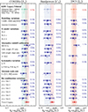 |
Fig. G.1. Whisker diagram of S8 cosmological results presented in this work. Each panel shows the compilation of results for one of our two-point statistics, as annotated. In each panel, we show the fiducial constraints in the relevant statistic with coloured points (colour-coded by the statistic), and highlight the fiducial marginal HPDI with a band of the equivalent colour. We also highlight the marginal HPDI in S8 from Planck-Legacy (shaded red). All variations to our analysis are annotated, and values plotted in dark blue. We annotate each analysis variation with the difference (quantified using the Gaussian approximation to the Hellinger tension) that the resulting marginal mode/HPDI has with respect to the fiducial (dark blue) or Planck (red). |
In this section we show the S8 equivalent of our main whisker-diagrams, for comparison with previous work. Figure G.1 shows the constraints for our En, CE, and ξ± statistics, with all analysis variations included. The variability between the constraints is larger in this projection than in the Σ8 projections, due to shifting of the posterior mode along the σ8, Ωm degeneracy. Otherwise, we note that all conclusions of this work are unchanged when analysing the S8 space, rather than the Σ8 space.
G.2. Redshift distributions
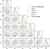 |
Fig. G.2. Posterior constraints on our redshift distribution bias parameters for chains utilising our various intrinsic alignment models. The filled contour shows the prior derived from our SKiLLS simulations. Smoothing kernels are matched between all contours (and marginal distributions), and are shown by the non-zero width of the σz = 0 contours/marginals. |
Figure G.2 shows the posterior constraints on our redshift distribution bias parameters, for chains analysed using various intrinsic alignment models, compared to the prior. The chains are all consistent with the prior, with only the low-z tomographic bins showing any tendency to shift away from the prior. Moreover, the posteriors are all fully consistent between the various analyses, demonstrating that the choice of intrinsic alignment model does not have a significant impact over the inferred redshift distribution biases.
G.3. Cosmological parameters
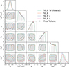 |
Fig. G.3. Posterior constraints on our cosmological parameters for chains utilising our various intrinsic alignment models. The filled contour shows the prior on each cosmological parameter. |
Figure G.3 shows the posterior constraints on our cosmological parameters, again for chains analysed using various intrinsic alignment models, and again compared to the prior. Only S8 and Ωm can be reliably considered to be constrained, although there are interesting preferences in certain parameters.
Appendix H: Tabulated constraints
Constraints on Σ8 under our analysis variations.
Appendix I: Post-unblinding analyses and changes
In this appendix we detail all analyses that were taken, and any changes that were made to the analysis and/or manuscript, after unblinding.
I.1. Comparison between Legacy and KiDS-1000
As discussed in Sect. 6, KiDS-Legacy presents a decrease in the marginal Hellinger tension with Planck of 2.2σ for Σ8 (1.65σ for S8). After the unblinding of KiDS-Legacy we investigated the differences between the Legacy and KiDS-1000 samples and analyses, to determine whether the change in cosmological parameters could be attributed to systematic or random variations. To do this, we reanalysed the KiDS-1000 and KiDS-Legacy shape catalogues with a series of analysis variations, which changed the sample used for cosmological inference and/or the analysis choices that were used in the inference. This required us, in each case, to rerun our N(z) estimation, our correlation function measurement, covariance computation, and posterior inference. We did not, however, remeasure the redshift distribution bias parameters or the multiplicative shape measurement biases for every setup.
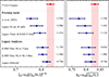 |
Fig. I.1. Variation in recovered En cosmological constraints for Σ8 (left) and S8 (right) when moving between KiDS-1000 and KiDS-Legacy analyses, relative to the constraints from Planck (red). Each point is annotated with the Hellinger tension between the marginal constraint and that of Planck. |
Figure I.1 presents a graphical summary of the changes we found in our recovered cosmological constraints when analysing KiDS-1000 using Legacy analysis choices and calibration methods, and when analysing Legacy using subsets defined by the KiDS-1000 footprint and photo-z baseline. Our investigation of the consistency between the data from Li et al. (2023a) and Legacy was focussed on two areas: the impact of Legacy analysis choices and calibration methods, and the impact of the new on-sky area available to Legacy. We quantified the effect of each analysis variation by recomputing the Hellinger tensions with respect to Planck, as this allows us to circumvent the complex covariance between various analyses of KiDS-1000 and KiDS-Legacy.
As a result of this investigation, we found no evidence of statistically significant systematic biases in the sample and analysis of KiDS-Legacy. We determined that the primary differences between the cosmological results of Li et al. (2023a) and Legacy are attributable to changes to our redshift calibration sample and methodology, and to statistical noise driven by the new area available to KiDS-Legacy outside the KiDS-1000 footprint. We have made no changes to the analysis methodology of Legacy as presented in the main text after this investigation, and thus conclude that this suite of tests do not represent a possible source of bias in our blinded analysis.
I.1.1. Analysing KiDS-1000 with Legacy calibration methods
We started by investigating the impact of the updated redshift estimation and calibration methods of Wright et al. (2025) on the cosmological constraints of Li et al. (2023a). To do this we reran the entirety of the cosmic shear measurement from KiDS-1000, from raw shape catalogues to cosmological inference, incorporating our new redshift estimation and calibration methodologies (leveraging e.g. gold-weight and simulation construction with sample matching). In this analysis we computed revised redshift bias estimates using the original KiDS-1000 redshift calibration sample, but updating to SKILLS image simulations and gold-weight redshift distribution estimation. The result of this end-to-end reanalysis are provided in Fig. I.1 as ‘Legacy Nz est. & calib.’. We found that the updated redshift distribution calibration method brings the cosmological estimates from the Li et al. (2023a) sample into better agreement with Planck, at 2.08σ consistency in Σ8 and 1.42σ consistency in S8. Importantly, both of these measurements satisfy the typical KiDS threshold for consistency of 2.3σ (equivalent to a one-sided probability to exceed of 0.01).
I.1.2. Updating KiDS-1000 to the Legacy calibration sample
We also measured the contribution to the difference between KiDS-1000 and KiDS-Legacy caused by the differences to our analysis choices and calibration sample, including our new tomographic bin limits and our greatly expanded redshift calibration dataset. To do this we again performed a full end-to-end reanalysis of KiDS-1000, this time with our new tomographic bin limits (excluding the sixth bin), and new redshift calibration sample from KiDZ. In this analysis we assume the redshift distribution biases and multiplicative shear biases are the same as the fiducial KiDS-Legacy analysis. We find that the use of the larger KiDZ calibration sample also slightly reduces the offset with Planck, to 1.61σ consistency in Σ8 and 1.12σ consistency in S8 (‘Legacy Tomo. & KiDZ (5 bins)’). This demonstrates that the KiDS-1000 sample, when analysed with our larger spectroscopic calibration sample and new redshift calibration methods (but without adding higher redshift sources, or using updated imaging, or new photo-z, or additional area) is consistent with the results from Planck and with the results from Legacy.
I.1.3. Legacy analysis in the KiDS-1000 volume
We explored the consistency between the constraints from KiDS-1000 and KiDS-Legacy by analysing the two samples in the same volume, and with the same analysis choices. We were able to do this fairly easily thanks to our analysis from Sect. I.1.2, which homogenised the tomography and N(z) estimation and calibration between the two samples. By restricting KiDS-Legacy to only the footprint of KiDS-1000, excluding the sixth tomographic bin, and using the NLA IA model, we were able to perform a comparison that is mostly free of statistical fluctuations. In fact there are still differences in the source samples due to changes in source extraction, image masking, source selection, and more, which we assumed add only a small amount of statistical noise to the comparison. We find that the Legacy sample in the same volume as KiDS-1000 is slightly closer to Planck than KiDS-1000, with a 1.17σ consistency in Σ8 and 0.85σ consistency in S8. This indicates that the sum total of changes (such as updated imaging calibrations, photo-z, masking, etc.) lead to a 0.44σ (0.27σ) decrease in the Hellinger distance between Planck and KiDS; significantly less than the change introduced by our new calibration methods.
I.1.4. Sixth tomographic bin and NLA-M
We further investigated the influence of adding the sixth tomographic bin and our new NLA-M IA model to the analysis of Legacy in the footprint of KiDS-1000 (‘K1000 Tiles; NLA-M; 6 bins’), finding that these changes caused a significant reduction in our marginal uncertainties (as expected) but did not lead to a significant change in the estimated cosmological parameters. As such, our Hellinger distance with Planck increases with these additions, to 1.40σ consistency in Σ8 and 1.00σ consistency in S8.
I.1.5. Additional Legacy area
Finally, we added the data back into Legacy that resides outside the footprint of KiDS-1000, and recover our fiducial result, which exhibits a 0.73σ consistency in Σ8 and 0.74σ consistency in S8. This demonstrates that there is a non-negligible statistical noise component in the difference between the sources probed within the footprint of KiDS-1000 and over the final KiDS-Legacy area.
I.2. Expanded scale cuts
Post unblinding, we discovered a typographical error in the pipeline which performed the measurement of correlation functions with expanded scale cuts (Sect. 5.2.7). This error meant that the pre-unblinding measurements were made with uncalibrated shapes directly from our shape measurement code lensfit, rather than with the recalibrated shapes (Sect. 3.5). We reran the expanded scale cut analysis with the correct recalibrated shapes post-unblinding, finding that the consistency between the analyses with fiducial and expanded scale cuts improved from 0.3σ to 0.15σ with the use of the correct shapes. No conclusions were changed as a result of this error.
I.3. Iterative covariances
All fiducial chains were recomputed using our iterative covariance framework post-unblinding. This was a conscious pre-unblinding choice, as the iterative covariances require non-negligible CPU time for the computation of MAP and new covariances. We found that this process had a negligible impact on our constraints (see Sect. 5.2.3), and thus does not represent a possible source of bias in our blinded analysis.
All Tables
Subtracted additive shear per ellipticity component, tomographic bin, and hemisphere.
Early-type galaxy sample properties for the mass-dependent intrinsic alignment model per tomographic bin.
All Figures
|
Fig. 1. Integrands of the transformation between the angular power spectrum and En/Bn (Eq. 17, panel ‘a’), CE, B (Eq. C.5, panel ‘b’), and ξ± (Eq. 15, panels ‘c’ and ‘d’). All solid integrands are normalised by their maximum absolute value. For both COSEBIs and 2PCFs, we show the limiting ranges of the statistics (n ∈ {1, 6} for En and θ ∈ {2.0, 300.0} arcmin for ξ±). For CE, B we show all eight bins used in KiDS-Legacy, defined between ℓ = 100 and ℓ = 1500. Note that, unlike previous KiDS analyses, our new treatment of T(θ) means that the CE, B initially go to zero within their desired ℓ ranges. |
| In the text | |
|
Fig. 2. Distribution of the mean weight of the KiDS-Legacy source galaxies in on-sky bins (0.1 × 0.1 degrees). The weights here include both shape measurement weights (Sect. 3.5) and redshift distribution gold weighting (Sect. 3.4). |
| In the text | |
|
Fig. 3. Left:N(z) used in the fiducial cosmic shear analyses of KiDS-Legacy. Each panel is one tomographic bin whose definition is determined by the grey band in photo-z. The N(z) have been shifted according to the mean bias estimated using our SKiLLS simulations, making each N(z) a correct representation of the effective N(z) that is used in the cosmological analyses. Fiducial biases are provided in Table 1. Right:δz correlation matrix for our fiducial N(z) (δzSOM, lower triangle) and the correlation matrix inferred from our cross correlation N(z) on the data (DzCC, upper triangle). |
| In the text | |
|
Fig. 4. PSF leakage measured in the KiDS-Legacy lensing sample after recalibration of shapes, computed per tomographic bin and ellipticity component k, and following the first-order systematics model in Eq. (24). |
| In the text | |
|
Fig. 5. Average of each ellipticity component in bins of the focal plane, for sources in all tomographic bins, relative to the (weighted) dispersion of ellipticities in the same bin. The weighted ellipticity dispersion per component over the bins in the focal plane are 0.287 ± 0.001 and 0.288 ± 0.001, indicating that the observed pattern is not driven by variable ellipticity dispersion across the focal plane. The figures still indicate the presence of the two-dimensional pattern reported in Figure 2 of Hildebrandt et al. (2020). |
| In the text | |
|
Fig. 6. Contributions to the additive systematic |
| In the text | |
|
Fig. 7. Ratio of PSF contamination in the cosmic shear correlation function, |
| In the text | |
|
Fig. 8. COSEBIs B modes measured in KiDS-Legacy. Each panel is annotated with the p-value of the B-mode signals for twenty modes (black) and our fiducial 6 modes (blue). The total p-value for the full data vector, also for six and twenty modes, is annotated in the upper right corner of the figure. The B-mode signals are highly correlated across modes within a tomographic bin, so readers are cautioned against so-called ‘χ-by-eye’. |
| In the text | |
|
Fig. 9. Fiducial Ωm, S8 (left), and Ωm, σ8 (right) constraints for our fiducial two-point statistics (En and CE, orange and purple respectively), compared to the CMB results from Planck-Legacy (red). The grey contours outline the marginal distribution of our a priori volume, with (inner) 1σ and (outer) 2σ boundary levels. |
| In the text | |
|
Fig. 10. Data vector and TPDs for the fiducial analysis of En (upper panel) and CE (lower panel). TPDs are shown as polygons spanning the 68th (red), and 95th (orange) percentiles of the posterior models. The En signals are highly correlated across modes within a tomographic bin, so readers are cautioned against so-called ‘χ-by-eye’. The bin 2 autocorrelation signal, for example, is consistent with the best fit model (PTE = 0.09), despite the apparent divergence of the data from the model. The overall PTEs for the full tomographic dataset in each statistic are provided in Table 4. |
| In the text | |
|
Fig. 11. Whisker diagram of Σ8 cosmological results presented in this work. The best-fitting α used for each statistic is annotated on the x-axis. Each panel shows the compilation of results for one of our two-point statistics, as annotated. In each panel, we show the fiducial constraints in the relevant statistic with coloured points (colour-coded by the statistic), and highlight the fiducial marginal HPDI with a band of the equivalent colour. We also highlight the marginal HPDI in Σ8 from Planck-Legacy (shaded red). All variations to the analysis are annotated, with the difference relative to the fiducial result quantified using the metric (Σ8fid − Σ8var)/σΣ8var (listed in blue). The Hellinger tension between the fiducial analyses and Planck is annotated in red. |
| In the text | |
|
Fig. 12. Constraints on the total intrinsic alignment amplitude from the various intrinsic alignment models, per tomographic bin (where appropriate), computed using the En posteriors. Bands and error bars represent the 1σ posterior constraint on each model. Our NLA-M model (red) is shown per tomographic bin, with the point positioned at the mean photo-z of the bin. |
| In the text | |
|
Fig. 13. Comparison of the marginal constraints on Ωm and S8 (top) and log10(TAGN/K) (bottom) when using a wider range of scales ( |
| In the text | |
|
Fig. 14. Comparison between KiDS-Legacy En cosmological constraints and recent stage-III cosmic shear survey results from the literature. We show the 2D posteriors for each analysis Ωm, S8 (left) as well as the marginal projections in Σ8 (α = 0.58, middle), and S8 (right). The 1D marginal ‘whisker’ plots are annotated as previously: circular points represent marginal mode and HPD intervals, while diamonds represent maximum a posteriori points and their associated PJ-HPD. Values are all calculated directly from the chains released by each analysis/survey, and in all cases except Legacy we take the MAP directly from the chain. We see that all surveys presented here are consistent with both KiDS-Legacy (black annotations) and Planck (red annotations) using our fiducial consistency metric of |ΔX|≤2.6σ (where X is either Σ8 or S8), as estimated using the Hellinger tension between marginal mode summaries. |
| In the text | |
|
Fig. 15. Upper panel: Estimate of the systematic uncertainty in our modelling of the matter power spectrum using CAMB and HMCODE2020, compared to two P(k) emulators BACCO (green) and EUCLIDEMULATOR2 (orange). The figure shows the ratio between the power spectrum from CAMB and HMCODE2020 to those returned by each emulator, evaluated at 10 000 representative samples from the fiducial En/Bn posterior with a tenth of a standard-deviation. Lower panel: Constraints on baryonic feedback suppression from KiDS-Legacy. The marginal HPDI of feedback amplitudes from our fiducial En/Bn is shown in red, relative to a range of hydrodynamical models of baryonic feedback suppression from FLAMINGO(Schaye et al. 2023). |
| In the text | |
|
Fig. D.1. Cartesian spatial map (corresponding Nside = 1024, showing a local flat projection of the healpix map) of the TG weights, wTG, throughout a single field of our KiDS-Legacy-like mock catalogue. Larger TG weights correspond to a higher local source density. |
| In the text | |
|
Fig. D.2. Dependence of the galaxy density, neff, on TG weights, wTG in the KiDS-Legacy-like mock catalogue. The data points represent the mean neff of ten equi-populated bins in wTG. The solid line shows the linear fit to the aforementioned data points of their respective tomographic bin, labelled S1-S6. The dashed horizontal lines show the mean values of neff calculated from the galaxy samples with variable depth per tomographic bin, while the dashed horizontal lines show the values of neff for the respective galaxy samples without any spatial variations in the observational depth. |
| In the text | |
|
Fig. E.1. Summary of our blinded B-mode investigation where we measure the COSEBIs En/Bn cosmic shear statistics, masking survey area where our astrometric metric, δrexp, exceeds a series of threshold values (shown on the x-axis). The middle panel shows the p-value that quantifies the likelihood that the B-mode is consistent with zero. As we reduce the δrexp threshold, the p-value increases above p ≤ 0.01 (red shaded region), and the masked survey passes the B-mode null test. As the mask reduces the total number of sources (lower panel), the blue squares show the p-values from a random mask analysis, demonstrating that the improved B-mode is not driven by a reduction in area. In the upper panel we find that the astrometric masking has a benign impact on our Σ8 cosmological constraints. The green data point and shaded regions shows the results from our fiducial analysis, demonstrating that failing data-vectors are consistent with our fiducial, all having less than 0.4σ changes in Σ8. |
| In the text | |
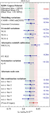 |
Fig. F.1. Whisker diagram of Σ8 cosmological results from ξ±. The figure is annotated as in Fig. 11. |
| In the text | |
|
Fig. F.2. Data vector and posterior predictive distributions for the fiducial run of our ξ±. Scales in the grey shaded region are excluded from our fiducial analysis. TPDs are shown for 68th (red) and 95th (orange) percentiles of the posterior models. |
| In the text | |
|
Fig. G.1. Whisker diagram of S8 cosmological results presented in this work. Each panel shows the compilation of results for one of our two-point statistics, as annotated. In each panel, we show the fiducial constraints in the relevant statistic with coloured points (colour-coded by the statistic), and highlight the fiducial marginal HPDI with a band of the equivalent colour. We also highlight the marginal HPDI in S8 from Planck-Legacy (shaded red). All variations to our analysis are annotated, and values plotted in dark blue. We annotate each analysis variation with the difference (quantified using the Gaussian approximation to the Hellinger tension) that the resulting marginal mode/HPDI has with respect to the fiducial (dark blue) or Planck (red). |
| In the text | |
|
Fig. G.2. Posterior constraints on our redshift distribution bias parameters for chains utilising our various intrinsic alignment models. The filled contour shows the prior derived from our SKiLLS simulations. Smoothing kernels are matched between all contours (and marginal distributions), and are shown by the non-zero width of the σz = 0 contours/marginals. |
| In the text | |
|
Fig. G.3. Posterior constraints on our cosmological parameters for chains utilising our various intrinsic alignment models. The filled contour shows the prior on each cosmological parameter. |
| In the text | |
|
Fig. I.1. Variation in recovered En cosmological constraints for Σ8 (left) and S8 (right) when moving between KiDS-1000 and KiDS-Legacy analyses, relative to the constraints from Planck (red). Each point is annotated with the Hellinger tension between the marginal constraint and that of Planck. |
| In the text | |
Current usage metrics show cumulative count of Article Views (full-text article views including HTML views, PDF and ePub downloads, according to the available data) and Abstracts Views on Vision4Press platform.
Data correspond to usage on the plateform after 2015. The current usage metrics is available 48-96 hours after online publication and is updated daily on week days.
Initial download of the metrics may take a while.