| Issue |
A&A
Volume 703, November 2025
|
|
|---|---|---|
| Article Number | A87 | |
| Number of page(s) | 7 | |
| Section | Stellar structure and evolution | |
| DOI | https://doi.org/10.1051/0004-6361/202555119 | |
| Published online | 07 November 2025 | |
Phase-resolved optical spectroscopy of the rapidly varying white dwarf ZTF 1851+1714
1
Department of Materials and Production, Aalborg University, Fibigerstræde 16, 9220 Aalborg, Denmark
2
Niels Bohr Institute, University of Copenhagen, Jagtvej 128, 2200 Copenhagen N, Denmark
3 Cosmic DAWN Center
4
INAF, Osservatorio Astronomico di Capodimonte, Salita Moiariello16, I-80131 Napoli, Italy
5
DARK, Niels Bohr Institute, University of Copenhagen, Jagtvej 128, 2200 Copenhagen N, Denmark
6
Nordic Optical Telescope, Rambla José Ana Fernández Pérez 7, local 5, E-38711 San Antonio, Breña Baja, Santa Cruz de Tenerife, Spain
⋆ Corresponding author: This email address is being protected from spambots. You need JavaScript enabled to view it.
Received:
11
April
2025
Accepted:
29
September
2025
Abstract
We report on phase-resolved optical spectroscopy and photometry in the R and B bands of the white dwarf candidate ZTF 185139.81+171430.3. The source has been reported to be variable with a large amplitude of close to 1 magnitude, in the R band, and a short period of 12.37 min. We confirm this period and interpret it as the spin period of the white dwarf. The optical spectrum shows emission lines from hydrogen and helium superposed on a featureless continuum. The continuum changes shape throughout a cycle, such that it is redder when the source is bright. There is tentative evidence for Doppler shifts in the emission lines during the spin cycle with an amplitude of a few tens of km s−1. Notably, the Hα and Hβ lines exhibit different radial velocity amplitudes, suggesting that they come from different emission regions. We also identify a candidate orbital period of 1.00 h, based on potential orbital sidebands. These features – Doppler shifts modulated at the spin frequency, brightness variations, and continuum shape changes – are consistent with the accretion curtain model, in which material is funneled from a truncated inner disc along magnetic field lines onto the magnetic poles of the white dwarf.
Key words: binaries: general / binaries: spectroscopic / stars: individual: ZTF 1851+1714 / white dwarfs
© The Authors 2025
 Open Access article, published by EDP Sciences, under the terms of the Creative Commons Attribution License (https://creativecommons.org/licenses/by/4.0), which permits unrestricted use, distribution, and reproduction in any medium, provided the original work is properly cited.
This article is published in open access under the Subscribe to Open model. This email address is being protected from spambots. You need JavaScript enabled to view it. to support open access publication.
1. Introduction
Cataclysmic variables (CVs) are close binary systems comprising a white dwarf (WD) accreting material from a companion star, typically a late-type main-sequence star (Robinson 1976; Angel 1978). Among CVs, magnetic systems are categorised based on the strength of the WD’s magnetic field, influencing the accretion dynamics and resulting observational characteristics. Two primary sub-classes are polars and intermediate polars, distinguished by their magnetic field intensities and accretion mechanisms (e.g., Piirola et al. 2008, and references therein).
In polars, also known as AM Herculis systems, the WD possesses a strong magnetic field (typically of 10–100 MG) that prevents the formation of an accretion disc. Instead, material from the donor star is channeled along magnetic field lines directly onto the magnetic poles of the WD. Furthermore, the spin and orbital periods are synchronised due to the magnetic field of the WD extending to, and coupling with that of, the secondary star. Typical spin and orbital periods are ∼1.3–8 h (some polars have been found to be slightly asynchronous with Pspin/Porb ∼ 0.8028 − 1.0028, see Schwope 2025). The accretion process leads to high-velocity infall, producing distinctive optical spectra characterised by strong emission lines, particularly of hydrogen and helium, and significant polarisation due to cyclotron radiation. Radial velocity studies in polars reveal complex line profiles influenced by the magnetic accretion geometry and the orbital motion of the binary components (Oliveira et al. 2017, 2020). See Cropper (1990) for an overview of polars.
Intermediate polars (IPs), or DQ Herculis stars, feature WDs with moderately strong magnetic fields (1–10 MG) and unlike for the polars, the spin and orbital period are asynchronous. Their orbital periods lie in the range ∼1.35–15.42 h1, and the spin periods are often Pspin ≲ 0.1Porb (Mukai 2017). In these systems, an accretion disc may form but is truncated at the inner regions by the magnetic field. The material is then funneled along magnetic field lines onto the WD’s magnetic poles. Optical spectra of IPs exhibit prominent emission lines, including He II 4686 Å, indicative of high-energy processes near the WD’s surface. Radial velocity measurements in IPs often show periodic variations that correspond to both the orbital period and the spin period of the WD, reflecting the asynchronous rotation typical of these systems (Patterson 1994).
Recent discoveries have introduced the concept of ‘WD pulsars’ exemplified by systems like AR Scorpii and J191213.72−441045.1 (Marsh et al. 2016; Pelisoli et al. 2023). In these binaries, the WD exhibits rapid rotation and a strong magnetic field, leading to radio pulsar-like emissions powered by the WD’s spin-down energy rather than accretion. However, interaction with the companion seems to be necessary to produce the pulse mechanism, unlike for regular pulsars. This suggests that a WD-pulsar is a result of CV evolution, as is proposed by Schreiber et al. (2021). To emphasise this nature, we mention the specifics of AR Sco, which is a binary system composed of a WD and an M5 dwarf with an orbital period of 3.56 h. There is also a 1.95 min variation in the flux from AR Sco, which is interpreted as the spin period of the WD. The strong magnetic field of the WD is believed to generate synchrotron emission via charged particles coming from the companion M-dwarf.
Kato & Kojiguchi (2021) discuss the nature of the variable source ZTF 185139.81+171430.3 (ZTF 1851+1714), which was first detected by the Zwicky Transient Factory (Ofek et al. 2020). The source has a short period of only 12.37 min and a large amplitude in its photometric light curve of almost 1 magnitude as reported by Kato & Kojiguchi (2021). The short period and large amplitude make the source rather unique and raise a question about its nature. They argue that the source most likely is a WD pulsar similar to AR Sco (Marsh et al. 2016), where the 12.37 min variability for ZTF 1851+1714, in a similar manner, reflects the spin period of a WD in a binary. ZTF 1851+1714 has also been detected in the X-rays, where it has been found to have a luminosity 400 times larger than that of AR Sco (Klingler & Pavlov 2021).
To investigate the nature of the system, we decided to perform phase-resolved optical spectroscopy and photometry in two bands of ZTF 1851+1714 as a project during a summer school at the Nordic Optical Telescope in August 2024. To our knowledge, no spectroscopic observations of ZTF 1851+1714 have been presented in the literature prior to our study.
2. Observations and data reduction
The main objective of our observing campaign was to secure phase-resolved spectroscopy of the system. Given the size of the telescope (main mirror 2.56-m) and the magnitude of the source (ranging between 18th and 19th magnitude), we were restricted to using low-resolution long-slit spectroscopy. We observed with the instrument ALFOSC and grism 19, which with a 1 0 slit provides an average resolution of 970 (or 300 km s−1 full-width-at-half-maximum, FWHM) over the spectral range from 4400 Å to 6770 Å2. To reduce read-out time we decided to bin the detector by a factor of two along the dispersion axis and to only read out a 500 pixel wide region along the slit. Before observing, we precisely timed the duration of the readout of the CCD for this setup so that we could calculate the exposure time that would ensure that after five spectra, we would be back at the same position in the phase, assuming a period of 12.37 min (Kato & Kojiguchi 2021). The measured read-out time was 8.38 ± 0.01 s. For five exposures, the exposure time was calculated by dividing the estimated period by the number of exposures and subtracting the measured read-out time, resulting in an exposure time of 140 s.
We also observed the target with two other grisms (18 and 20) to be able to characterise the optical spectrum from about 3700 Å into the near-infrared at 9700 Å. The average spectral resolution of these grisms are 1000 and 770, respectively, again using a 1 0 wide slit2.
The slit was in all observations aligned with a nearby non-variable star, in order to have a comparison source for removing any trends from the individual spectra, related to changing airmass, seeing and similar effects, during the cycles. This comparison star is used in the analysis presented in Section 3.4, where the target spectra were normalised by the mean flux of the comparison star in the 5000–5500 Å region and subsequently scaled to match the flux level of the comparison star in the first group within the same region.
The observations were carried out at low airmass (see Table 1) and seeing was approximately 0 65 but varied in the interval 0
 60–0
60–0 74. The autoguider of the telescope keeps the source in a fixed position within the slit to a precision that is well below 0
 1, and therefore we do not expect spurious radial velocity signals from the source moving within the slit. The log of observations can be inspected in Table 1, and the precise start times for the 40 spectra obtained with grism 19 can be found in Table 2.
Log of ALFOSC observations in August 2024.
Start Universal Time (UT) for each of the 40 grism 19 exposures ordered by group, i.e. by phase.
We secured photometric light curves on two epochs in the Bessel B and R filters in order to examine the colour behaviour of the photometric variability. The observations were reduced using aperture photometry, and brightness variations were measured via differential photometry using the nearby comparison star. The exposure times and cadence of these observations are listed in Table 1.
The data were reduced using standard methods for wavelength calibration, extraction, and flux calibration in longslit spectroscopy as implemented in a Python code (Valeckas et al. 2025). Flux calibration was done using observations of spectrophotometric standard stars observed on the same nights as the science data.
3. Results
3.1. The full spectrum
In Fig. 1, we show the full optical spectrum covering the region of spectra from near-ultraviolet to near-infrared using spectra from all three grisms. As the object is likely far out (parallax of 0.325 ± 0.119 mas Kato & Kojiguchi (2021)), we have corrected the spectrum for a full line-of-sight foreground extinction in the direction of ZTF 1851+1714 of AV = 0.996 mag as determined from the extinction map of Schlafly & Finkbeiner (2011). The spectra taken with grism 19 were RV-corrected prior to being averaged. The spectrum is characterised by a large number of emission lines from H I, He I, and He II superposed on a fairly featureless continuum. The emission lines are resolved in velocity. Also the Hα and Hβ lines are prominent, where for Hα we measure a Gaussian width of 7.3 ± 0.3 Å corresponding to 750 km s−1 FWHM corrected for the spectral resolution. There are absorption features at 5890 Å and 6280 Å (in addition to absorption at the telluric A and B bands). The 5890 Å is presumably caused by interstellar Na, as no significant periodic variability is measured in its radial velocity; however, this interpretation remains tentative given the low spectral resolution and signal-to-noise ratio. The 6280 Å line is caused by telluric absorption due to oxygen.
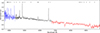 |
Fig. 1. Stacked spectrum using all exposures in all grisms. The blue section represents the grism 18 observation, the black spectrum the weighted mean of the 40 grism 19 spectra, and the red section represents the grism 20 spectrum. The positions of emission lines from H I, He I, and He II are indicated with vertical lines at the top. Some of the hydrogen lines in the grism 20 spectrum are only tentatively detected. We also mark the position of NaD absorption, which is presumably interstellar in nature. The spectrum has been normalised to 1 at 6000 Å. |
The presence of prominent hydrogen lines makes it unlikely that the 12.37 min variability reflects the orbital period. As we understand, CVs with hydrogen-rich donors have an observed orbital period minimum of approximately 78 − 82 min (Gänsicke et al. 2009). This minimum may be pushed to ∼51 min for extremely low-metallicity donors (Stehle et al. 1997), and potentially as low as ∼37 min if the companion is a degenerate object such as a brown dwarf or gas giant (Rappaport et al. 2021). Periods significantly below these thresholds require highly compact donors and are typically associated with helium dominated systems such as AM CVns, which typically show no hydrogen in their spectra. While trace amounts of hydrogen have been detected in the spectra of some AM CVn-type systems (e.g. HM Cnc; see Israel et al. 2002; Munday et al. 2022), the amount of hydrogen is estimated to be very low and the optical spectra remain helium dominated.
In the case of ZTF 1851+1714, the 12.37 min variability is well below these period limits, yet the optical spectrum is hydrogen-rich. This strongly suggests that the periodicity does not represent the orbital period of the system. Instead, we interpret it as the spin period of the WD.
3.2. Phase-resolved spectroscopy
The phase-resolved grism 19 spectra can be seen in Fig. 2. Here, we have stacked the spectra in five groups ordered by phase. Note that start time is arbitrary as we did not synchronise the start of the observations with the ephemeris of the variable as these are not known well enough to allow this. The spectra show a strong chromatic evolution during the phase: the continuum is significantly redder when the source is bright compared to the spectrum closer to minimum flux.
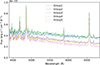 |
Fig. 2. Phase-resolved spectroscopy covering the spectral region from 4400 Å to 6770 Å using grism 19. We show the stacked spectra for each of the given groups covering the full phase of the 12.37 min variability period. |
We also measure the Doppler shifts of the emission lines. Only the Hα and Hβ lines have sufficient signal-to-noise ratio to allow a significant measurement, but for these two lines, we find fairly consistent results for all the spectra (see Fig. 3). The radial velocity of both of these lines vary sinusoidally with the observed period, meaning that they are related to the spin of the WD. This could indicate that they originate from where the material of the accretion disc is able to couple to the magnetic field of the WD and hence rotate with it. A difference in radial velocity amplitude is also apparent, which means that the two lines presumably originate from different places.
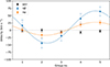 |
Fig. 3. Velocities derived from Doppler shifts measured from the Hα and Hβ lines covering the full phase of the 12.37 min variability period (see Fig. 2). Sine curves have been fitted to the Hα and Hβ data points to highlight their periodic nature. For comparison, we also show velocities measured from sky-lines in the same spectra. |
3.3. Equivalent width of the Hβ line
An empirical criterion for classifying magnetic CVs has also been suggested by Silber (1992). According to this criterion, the equivalent width (EW) of the Hβ line should be greater than 20 Å and the ratio between the amplitude of He II 4686 Å/Hβ > 0.4. Calculating these for each of the five spectra in Fig. 2, using Specutils (Lisa & Bot 2017), yields a mean EW of 29 ± 4 Å and a mean ratio He II 4686 Å/Hβ of 0.72 ± 0.04. These values are above the thresholds, even when considering errors, implying that ZTF 1851+1714 is a magnetic CV.
3.4. Variability analysis
In order to investigate the periodic variability in the magnitude of ZTF 1851+1714, we also looked at the 40 individual spectra and R and B band photometry. The spectra were produced in the same manner as the five spectra in Fig. 2, but the comparison star was used to further calibrate each spectrum, and they have not been corrected for foreground extinction. These spectra are noisier, which is expected, and they present some of the same features, mainly the Hα and Hβ lines and periodic flux variation.
The values of the integrated fluxes can be seen in Fig. 4. They were obtained by numerically integrating the spectra in their wavelength range, which is ∼4404 Å to ∼6964 Å. A clear sinusoidal variability is seen, corresponding to the eight periods observed. Another modulation, with a longer period of ∼0.6 h also appears to be present, looking at the dotted blue peaks around [0.2, 0.8, 1.4] h.
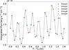 |
Fig. 4. Calculated integrated flux for each of the 40 spectra. Each spectrum has been numerically integrated in their wavelength range. The time assigned to each spectrum is the start time of the exposure. These timestamps were shifted such that the first measurement starts at 0. |
To investigate the potential different modulations, a fast Fourier transform (FFT) was used to produce a power spectrum of the integrated fluxes (Fig. 6). An oversampling factor of 20 was applied to improve frequency resolution, and the integrated flux values were normalised in terms of the maximum integrated flux, to minimise numerical errors. The frequency range of 3–12 h−1 was selected because the lower frequencies were too close to the total observation time, while the higher frequencies were close to the exposure times, making them less reliable. Furthermore, the power spectrum was normalised and a detection threshold corresponding to a 5% false-alarm probability (FAP) has been included to highlight the significance of peaks.
A clear dominant frequency is present corresponding to a period of 12.29 min, which matches the spin period of the WD (Kato & Kojiguchi 2021), to an error within 1%. No other modulations are immediately apparent.
To further investigate the periodic behaviour, we consider the presence of orbital sidebands. In intermediate polars, optical signals commonly exhibit orbital sidebands at ω − Ω, where ω represents the WD’s spin frequency and Ω denotes the orbital frequency (Patterson 1994). If the peak observed at 3.88 h−1 in the top panel of Fig. 6 corresponds to this orbital sideband, it implies an orbital frequency of Ω = 1.00 h−1, leading to an estimated orbital period of 1.00 h. Additionally, a peak at 7.76 h−1 is detected, which corresponds exactly to 2(ω − Ω). This suggests an ∼1 h orbital period for the binary system, although it cannot be definitively confirmed (see Section 4 for a discussion of this orbital period compared to those of known IPs).
The aliasing structure resulting from the spectral window of the 40 grism 19 spectra is overplotted with the power spectrum in the top panel of Fig. 6. It has been scaled by the same factor as the normalised power spectrum. It can be seen that the proposed orbital sideband at 3.88 h−1 lies close to an alias peak introduced by the spectral window, although the two do not exactly coincide. The feature at 7.76 h−1 is located further away from the nearest alias peaks. This makes it difficult to determine whether this represents a true periodic signal or is an artefact from the observation window. However, the peaks do not reach the detection threshold, making it even more uncertain whether they are indeed from a true periodic signal.
To investigate the wavelength-dependent variations in the spectra, we fitted straight lines to the different continua. This was done to estimate the slopes, which would give us a measure of whether the spectra were more blue or red. If the slope is negative, we have a bluer continuum, because this would mean that the flux is larger at lower wavelengths and drops off towards higher wavelengths. When the slope is positive, we have a redder spectrum, as the flux increases with wavelength. The resulting slope for each spectrum is shown in Fig. 5. They have been scaled in terms of the maximum value of 1.07 × 10⁻⁴ erg s−1 cm−2 Å−2, to highlight the periodic variation of the slope throughout the eight observed periods.
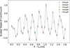 |
Fig. 5. Slopes of the continua for the different spectra, obtained by fitting a straight line to each spectrum. The values are scaled in terms of the continuum with the highest slope, such that this value equals one. |
Comparing Fig. 5 with Fig. 4, we find that when the integrated flux is low, the slopes tend to be negative, meaning that the spectra are bluer when there is a minimum in the integrated flux. The opposite is seen when the integrated flux is high, the slopes tend to be positive, and hence the spectra are redder. Additionally, a slight phase shift is present. In Fig. 5 the highest integrated flux values are mainly associated with group 1, whereas in Fig. 4, they are more strongly associated with group 2.
In order to see how the amplitude of the main four emission lines, He II, Hβ, He I, and Hα, varies compared to the continuum, we separated them from the continuum. This was done by fitting a polynomial to parts of the spectra without emission lines, thus obtaining a fit of the continuum. Subtracting this continuum from the spectra, we could fit Gaussian functions to each of the four lines. Integrating these fits for each of the spectra, we get Fig. 7. Here, it is seen that the emission lines do not show any periodic behaviour. However, because these lines have a much smaller area in terms of the calculated integrated flux, they are also more susceptible to noise, which is also evident from the error bars. It is also seen that the periodic behaviour of the WD is dominated by the continuum since the integrated fluxes correspond to those in Fig. 4.
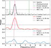 |
Fig. 6. Normalised FFT power spectra of the integrated fluxes seen in Fig. 4, along with the R and B band photometry measurements. The fluxes have been normalised in terms of the maximum flux. An oversampling factor of 20 has been used to get better frequency resolution in all three power spectra. The aliasing structure resulting from the spectral window of the observations for grism 19 is shown in the top panel, along with the potential orbital sidebands. The aliasing structure has been scaled by the same factor as the normalised power spectrum. A detection threshold corresponding to a 5% FAP has been calculated for each spectrum. |
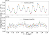 |
Fig. 7. Top: Estimated integrated fluxes for the continuum, which has been obtained by fitting a polynomial to the parts of the spectra, without emission lines. Bottom: Estimated integrated fluxes for the He II, Hβ, He I and Hα emission lines, obtained from the spectra by subtracting the continuum and fitting Gaussian functions to each of the four lines. |
3.5. Photometry
To build on the findings of the integrated spectra, we took photometric measurements in the R and B bands (see Fig. 8). This was done to compare the results and to investigate orbital sidebands by making FFT power spectra. A total of 70 measurements were made in both bands with exposure times of 50 s, which means ∼1 h of observation time, covering ∼ five spin periods of the WD.
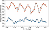 |
Fig. 8. R and B band photometry measurements, displayed by red and blue dots, respectively. The R band measurements were taken on August 25 2024 and the B band measurements on August 23 2024. The magnitudes are displayed in terms of the difference between ZTF 1851+1714 and the reference star. |
The same periodic behaviour as in Fig. 4 is present in the R band, however, no other modulations are found upon visual inspection. Looking at the power spectrum for the R band in Fig. 6 confirms that the dominating period is the spin period of the WD.
In the B band measurements, many different modulations are present, but the previous periodic behaviour of the WD spin is not immediately apparent. Examining the power spectrum, a peak was found close to the frequency corresponding to the spin period of the WD. However, the peaks are less prominent than for the R band measurements, making it difficult to determine anything with confidence. This is also evident from the fact that none of the peaks reach the detection threshold.
4. Discussion
The changing shape and luminosity of the continuum during the 12.37 min variability period require explanation. If it were a hot spot on the WD, we would see the opposite trend: bluer spectrum correlating with a higher luminosity. If there was a cold spot we would expect the same trend: the luminosity would be lower when the cold spot was on the line of sight. One explanation could be a non-thermal source of continuum, i.e. synchrotron or cyclotron emission. Another possibility would be occultation of a red source in the faint state, i.e. occultation of a red companion star, but the light curve does not look like that of an eclipsing binary.
A more plausible explanation involves the accretion geometry close to the WD, where the accretion disc is truncated. The periodic variations in the velocities of the Hα and Hβ emission lines, derived from Doppler shifts, confirm that we are receiving light from this region, as they follow the same periodic behaviour as the WD.
In the accretion curtain scenario, the matter from the disc is funneled along the WD’s magnetic field lines, forming a curtain-like structure that channels material onto the magnetic poles. This model suggests that we receive more light when viewing these curtains from the side, specifically when the magnetic poles are not pointing directly towards us, because a larger emitting surface area is exposed (see Chapter 9 in Hellier 2001).
This would imply that, when the integrated flux is at maximum, we might not see the hot spot directly, leading to a redder spectrum. Conversely, when the magnetic pole is directed towards us, some of the light is absorbed or scattered within the curtain, reducing the integrated flux. However, since the pole is facing us in this phase, we observe an increase at blue wavelengths as the hot spot is visible.
A slight phase shift is observed between the integrated flux and the radial velocities of the Hα and Hβ emission lines. Although the lines are generally blueshifted near flux maximum and redshifted near flux minimum, this correspondence is not exact. As is seen in groups 4 and 5 of Fig. 2 and Fig. 3, the maximum redshift occurs just after the flux minimum. This offset is consistent with the accretion curtain model; as the magnetic pole and curtain rotate and point towards us, the continuum flux drops due to increased absorption or scattering, and shortly thereafter the curtain’s motion leads to a redshift, as it is moving away from us. Likewise, as the curtain rotates and points away from us, the emitting area increases, the flux reaches a maximum, and the inflowing material begins moving towards us again, producing a blue shift. A similar phase relationship is observed in the intermediate polar EX Hydrae (Mhlahlo et al. 2007).
Furthermore, Mhlahlo et al. (2007) argue that the Doppler shift of the Hβ line in EX Hydrae originates from the rotation of the funnel at the outer disc edge, where a shock is created, while the Doppler shift of the narrow component of the Hα line originates from the flow of material along the field lines in the curtain. This could explain the amplitude difference that we see for ZTF 1851+1714, since the Hβ line obtains higher radial velocities. It is also plausible that this shock causes an increase in the received flux at the blue wavelength during minimum of the integrated flux, as it would be facing us, while at maximum the funnel overshadows it, resulting in a redder spectrum.
In terms of the variability analysis of the integrated spectra and the photometry of the R and B band, we find the same periodic variability as in Kato & Kojiguchi (2021), which is believed to be the WD spin period. Additional periodic modulations at 3.88 h−1 and 7.76 h−1 were present, which could be related to an orbital sideband if the binary has an orbital period of ∼1.00 h. Although it is theoretically possible to have orbital periods down to ∼37 min with a brown dwarf companion (Rappaport et al. 2021), it seems unlikely for ZTF 1851+1714 to have such an orbital period, considering those of the current, classified intermediate polars, which range from 1.35–15.42 h. The absence of orbital sidebands in most measurements further supports the conclusion that the modulation is not directly linked to the orbital dynamics of the binary system.
The limited time spans of the observations also restrict our sensitivity to long-period modulations. To better constrain the orbital period and potential sidebands, additional observations are needed, ideally spanning multiple nights and covering several WD spin cycles to reduce aliasing effects. A higher number of phase-resolved spectra covering the spin period of the WD would improve our ability to track spectral variations over time, allowing for a more detailed characterisation of how the observed features evolve throughout the period. High resolution phase-resolved spectroscopy would enable a more detailed study of emission regions and potentially allow for Doppler tomography (Kotze et al. 2016). Polarimetric observations could further constrain the magnetic geometry and test for spin-modulated polarisation.
Previous X-ray observations using the Swift X-Ray Telescope were reported by Klingler & Pavlov (2021), but these data were not examined for the presence of orbital sidebands. Since intermediate polars often show clear X-ray modulations at the WD spin period and potentially at sideband frequencies, re-analysis of the Swift data, or deeper follow-up with current X-ray observatories, could provide an independent check on the proposed ∼1.00 h orbital period.
5. Conclusion
The observational properties of ZTF 1851+1714 are best explained by a geometry consistent with an intermediate polar. The periodic behaviour of the continuum and emission lines and the observed colour variations all support a scenario in which accretion is controlled by a magnetic field that truncates the inner disc and channels material along field lines to the WD poles.
The phase-dependent blue and red continuum behaviour can be explained by the variable visibility of the hot spot and accretion curtain, and the behaviour of the Doppler shifted emission lines is consistent with flow patterns seen in other intermediate polars such as EX Hydrae. The absence of eclipses, the short photometric period, and the spectroscopic characteristics all argue against other interpretations, such as WD pulsations or a simple binary eclipse.
Although some features, particularly the orbital period, remain uncertain, ZTF 1851+1714 shows strong similarities to known intermediate polars and is a compelling candidate for inclusion in this class. Follow-up observations across multiple wavelengths and longer baselines will be essential to confirm this classification and further understand the structure of the system.
Acknowledgments
Based on observations made with the Nordic Optical Telescope, owned in collaboration by the University of Turku and Aarhus University, and operated jointly by Aarhus University, the University of Turku and the University of Oslo, representing Denmark, Finland and Norway, the University of Iceland and Stockholm University at the Observatorio del Roque de los Muchachos, La Palma, Spain, of the Instituto de Astrofisica de Canarias. The data presented here were obtained with ALFOSC, which is provided by the Instituto de Astrofisica de Andalucia (IAA) under a joint agreement with the University of Copenhagen and NOT. JPUF is supported by the Independent Research Fund Denmark (DFF–4090-00079) and thanks the Carlsberg Foundation for support. The authors would like to thank the participants of the NOT Summer School 2024 who offered valuable discussions and insights that helped shape the direction of this work.
References
- Angel, J. R. P. 1978, ARA&A, 16, 487 [NASA ADS] [CrossRef] [Google Scholar]
- Cropper, M. 1990, Space Sci. Rev., 54, 195 [CrossRef] [Google Scholar]
- Gänsicke, B. T., Dillon, M., Southworth, J., et al. 2009, MNRAS, 397, 2170 [NASA ADS] [CrossRef] [Google Scholar]
- Hellier, C. 2001, Cataclysmic Variable Stars (Springer) [Google Scholar]
- Israel, G. L., Hummel, W., Covino, S., et al. 2002, A&A, 386, L13 [NASA ADS] [CrossRef] [EDP Sciences] [Google Scholar]
- Kato, T., & Kojiguchi, N. 2021, arXiv e-prints [arXiv:2107.09913] [Google Scholar]
- Klingler, N., & Pavlov, G. 2021, ATel, 14965, 1 [Google Scholar]
- Kotze, E. J., Potter, S. B., & McBride, V. A. 2016, A&A, 595, A47 [NASA ADS] [CrossRef] [EDP Sciences] [Google Scholar]
- Lisa, M., & Bot, H. 2017, My Research Software https://github.com/github-linguist/linguist [Google Scholar]
- Marsh, T. R., Gänsicke, B. T., Hümmerich, S., et al. 2016, Nature, 537, 374 [NASA ADS] [CrossRef] [Google Scholar]
- Mhlahlo, N., Buckley, D. A. H., Dhillon, V. S., et al. 2007, MNRAS, 378, 211 [NASA ADS] [CrossRef] [Google Scholar]
- Mukai, K. 2017, PASP, 129, 062001 [Google Scholar]
- Munday, J., Marsh, T. R., Hollands, M., et al. 2022, MNRAS, 518, 5123 [Google Scholar]
- Ofek, E. O., Soumagnac, M., Nir, G., et al. 2020, MNRAS, 499, 5782 [NASA ADS] [CrossRef] [Google Scholar]
- Oliveira, A. S., Rodrigues, C. V., Cieslinski, D., et al. 2017, AJ, 153, 144 [NASA ADS] [CrossRef] [Google Scholar]
- Oliveira, A. S., Rodrigues, C. V., Martins, M., et al. 2020, AJ, 159, 114 [Google Scholar]
- Patterson, J. 1994, PASP, 106, 209 [Google Scholar]
- Pelisoli, I., Marsh, T. R., Buckley, D. A. H., et al. 2023, Nat. Astron., 7, 931 [NASA ADS] [CrossRef] [Google Scholar]
- Piirola, V., Vornanen, T., Berdyugin, A., Coyne, G. V., & Ja, S. 2008, ApJ, 684, 558 [Google Scholar]
- Rappaport, S., Vanderburg, A., Schwab, J., & Nelson, L. 2021, ApJ, 913, 118 [Google Scholar]
- Robinson, E. L. 1976, ARA&A, 14, 119 [Google Scholar]
- Schlafly, E. F., & Finkbeiner, D. P. 2011, ApJ, 737, 103 [Google Scholar]
- Schreiber, M. R., Belloni, D., Gänsicke, B. T., Parsons, S. G., & Zorotovic, M. 2021, Nat. Astron., 5, 648 [NASA ADS] [CrossRef] [Google Scholar]
- Schwope, A. D. 2025, A&A, 698, A106 [NASA ADS] [CrossRef] [EDP Sciences] [Google Scholar]
- Silber, A. D. 1992, Ph.D. Thesis, Massachusetts Institute of Technology [Google Scholar]
- Stehle, R., Kolb, U., & Ritter, H. 1997, A&A, 320, 136 [NASA ADS] [Google Scholar]
- Valeckas, K., Fynbo, J. P. U., Krogager, J. K., & Heintz, K. E. 2025, https://doi.org/10.5281/zenodo.15091603 [Google Scholar]
All Tables
Start Universal Time (UT) for each of the 40 grism 19 exposures ordered by group, i.e. by phase.
All Figures
|
Fig. 1. Stacked spectrum using all exposures in all grisms. The blue section represents the grism 18 observation, the black spectrum the weighted mean of the 40 grism 19 spectra, and the red section represents the grism 20 spectrum. The positions of emission lines from H I, He I, and He II are indicated with vertical lines at the top. Some of the hydrogen lines in the grism 20 spectrum are only tentatively detected. We also mark the position of NaD absorption, which is presumably interstellar in nature. The spectrum has been normalised to 1 at 6000 Å. |
| In the text | |
|
Fig. 2. Phase-resolved spectroscopy covering the spectral region from 4400 Å to 6770 Å using grism 19. We show the stacked spectra for each of the given groups covering the full phase of the 12.37 min variability period. |
| In the text | |
|
Fig. 3. Velocities derived from Doppler shifts measured from the Hα and Hβ lines covering the full phase of the 12.37 min variability period (see Fig. 2). Sine curves have been fitted to the Hα and Hβ data points to highlight their periodic nature. For comparison, we also show velocities measured from sky-lines in the same spectra. |
| In the text | |
|
Fig. 4. Calculated integrated flux for each of the 40 spectra. Each spectrum has been numerically integrated in their wavelength range. The time assigned to each spectrum is the start time of the exposure. These timestamps were shifted such that the first measurement starts at 0. |
| In the text | |
|
Fig. 5. Slopes of the continua for the different spectra, obtained by fitting a straight line to each spectrum. The values are scaled in terms of the continuum with the highest slope, such that this value equals one. |
| In the text | |
|
Fig. 6. Normalised FFT power spectra of the integrated fluxes seen in Fig. 4, along with the R and B band photometry measurements. The fluxes have been normalised in terms of the maximum flux. An oversampling factor of 20 has been used to get better frequency resolution in all three power spectra. The aliasing structure resulting from the spectral window of the observations for grism 19 is shown in the top panel, along with the potential orbital sidebands. The aliasing structure has been scaled by the same factor as the normalised power spectrum. A detection threshold corresponding to a 5% FAP has been calculated for each spectrum. |
| In the text | |
|
Fig. 7. Top: Estimated integrated fluxes for the continuum, which has been obtained by fitting a polynomial to the parts of the spectra, without emission lines. Bottom: Estimated integrated fluxes for the He II, Hβ, He I and Hα emission lines, obtained from the spectra by subtracting the continuum and fitting Gaussian functions to each of the four lines. |
| In the text | |
|
Fig. 8. R and B band photometry measurements, displayed by red and blue dots, respectively. The R band measurements were taken on August 25 2024 and the B band measurements on August 23 2024. The magnitudes are displayed in terms of the difference between ZTF 1851+1714 and the reference star. |
| In the text | |
Current usage metrics show cumulative count of Article Views (full-text article views including HTML views, PDF and ePub downloads, according to the available data) and Abstracts Views on Vision4Press platform.
Data correspond to usage on the plateform after 2015. The current usage metrics is available 48-96 hours after online publication and is updated daily on week days.
Initial download of the metrics may take a while.