© The Authors 2025

1 Introduction

High-precision polarimetry empowers astronomers to push the frontiers of their research fields. For example, the precision of a few parts per million (ppm) makes it possible to detect the polarization of reflected light from a hot Jupiter in unresolved observations of the host star (Seager et al. 2000; Bailey et al. 2018, 2021). High-precision polarimeters are anticipated.

PlanetPol, a pioneering high-precision optical polarimeter used in nighttime astronomy, was developed by Hough et al. (2006). A precision of ~1 ppm was achieved. The key technology is the high-speed modulation of polarization. PlanetPol uses a photoelastic modulator (PEM) that modulates the state of polarization (i.e., rotates the position angle of polarization) at a very high frequency (tens of kilohertz), which exceeds the timescale of turbulence in Earth’s atmosphere. Combined with a fixed polarizing filter (prism), the fluxes of orthogonally oriented light waves can be compared in the time domain. Thus, high-precision polarimetry was possible using a simple optical system.

Following PlanetPol, several fast-modulating high-precision polarimeters were developed: the HIgh Precision Polarimetric Instrument (HIPPI) (Bailey et al. 2015, 2017, 2020) and POLISH series (Wiktorowicz & Matthews 2008; Wiktorowicz & Nofi 2015; Wiktorowicz et al. 2023). The HIPPI series adopted a ferro-electric liquid crystal modulator instead of a PEM. Although liquid-crystal modulators have lower frequencies than PEMs by one or two orders of magnitude, Bailey et al. (2015) proved that liquid-crystal modulators are suitable for astronomical polarimters. POLISH2 uses differently oriented double PEMs and can simultaneously observe the full Stokes parameters q = Q/I, u = U/I, and v = V/I (Wiktorowicz & Nofi 2015), where the pair q and u describes the degree and position angle of linear polarization (LP), and v expresses the degree and handedness of circular polarization (CP).

Fast-modulating polarimeters require a light-sensing frequency that is faster than (or at least as fast as) the modulation frequency. Such high-speed light sensing is not possible with conventional charge-coupled device (CCD) cameras. Therefore, these fast-modulating polarimeters use avalanche photodiodes (APDs) or photomultiplier tubes (PMTs).

A disadvantage of APDs and PMTs is that they do not have spatial resolution (imaging capability). This significantly limits the scope of the scientific applications. For example, it is not possible to study spatial distribution of polarization on extended sources such as Solar System planets, comets, nebulae, and nearby galaxies. Another case where spatial resolution matters is lunar Earthshine polarimetry, conducted to investigate signatures of life and habitats (e.g., Sterzik et al. 2012, 2019; Bazzon et al. 2013; Miles-Páez et al. 2014; Takahashi et al. 2013, 2021). The key procedure in Earthshine data reduction is subtracting strongly scattered light from the Moon’s bright side. Since scattered light intensity depends highly on sky position, spatial resolution is desired.

However, recently, we observed the rapid evolution of high-speed imaging devices, such as electron-multiplying CCD (EM-CCD) cameras and complementary metal-oxide semiconductor (CMOS) cameras. Given the technological advances, we developed POlarimeter for Precision Observations (POPO). While POPO follows the core concept of the previous fast-modulating polarimeters, the light sensors are replaced by high-speed cameras. POPO aims to be a characteristic polarimeter with either a high precision (≲10 ppm) or a high time resolution (≲1 s) while having imaging capability. Fast-modulating polarimeters can achieve high time resolution instead of extreme precision. High time-resolution polarimetry may open up an unexplored field of study (Shearer et al. 2010).

This study reports on the basic performance of POPO. In Section 2, we describe the optical and control systems of POPO. After general explanations of the test observations in Section 3, data reduction methods are outlined in Section 4. We present the system characteristics (such as artificial polarization and response matrix) and performance (such as precision, accuracy, and stability) in Section 5, which follows concluding remarks in Section 6.

In this study, the Stokes parameters were defined either in a coordinate system fixed to POPO (referred to as the instrumental coordinate system) or in the equatorial coordinate system. In the former case, we denote the normalized Stokes parameters as $\hat{q},\hat{u}$, and $\hat{v}$; the reference of the polarization position angle is normal to the plane of Fig. 1 (light with a positive $\hat{q}$ is polarized normal to this plane or along the y axis of the view image). In the latter case, Stokes is denoted by q, u, and v, and the reference axis is the equatorial north-south axis.¹ The angle ρ represents the rotation angle of the instrumental rotator with respect to its mechanical origin, whereas the angle ϕ denotes the position angle of the instrumental reference axis (i.e., y axis of the view image) with respect to the equatorial north-south axis.

2 Instrumentation

The optical design and control system of POPO is visually illustrated in Fig. 1. The key components of the system are (1) a liquid-crystal variable retarder (LCVR), (2) a polarizing beam splitter (PBS), and (3) two high-speed cameras. Below are descriptions of each component.

1. A high-speed LCVR (Meadowlark Optics HLC-200-VIS) is placed right in front of the telescope focus with its fast axis tilted by 45° with respect to the instrumental reference axis (normal to the plane of Fig. 1). The retardance corresponding to the LCVR can be rapidly switched (up to a few hundreds of hertz) between zero and a half wavelength to modulate the polarization position angle of the incident light. More details are given in Appendix A.

2. A cubic PBS (SIGMAKOKI PBSW-20-3/7) transmits horizontally (with respect to the plane of Fig. 1) polarized light and reflects vertically polarized light. Two factors guided our choice of cubic PBS: (i) cubic PBSs create larger distances between split beams compared to Wollaston prisms (WPs), providing enough space to install the two cameras; (ii) WPs’ separation angle varies with wavelength causing chromatic aberration in broad-band images, while cubic PBSs have no wavelength dependence.

3. An electron-multiplying CCD camera (EM-CCD; Andor iXon Ultra 897) and a CMOS camera (Andor Zyla 4.2 PLUS) are installed at the focal point in the transmitted channel and in the reflected channel, respectively. These cameras are capable of high-speed imaging as fast as the LCVR. The timing of exposures by the two cameras must be synchronized with polarization modulation by the LCVR. This is made possible by sending trigger pulses to the cameras and the LCVR from a data acquisition device (DAQ; National Instruments USB-6211).

The optical system in the default configuration measures Stokes $\hat{q}$. Stokes $\hat{u}$ is measured when a 22.5°-tilted half-wave plate (HWP; Bolder Vision Optik AHWP3) is inserted in front of the LCVR because the HWP converts $\hat{u}$ into $\hat{q}$. Similarly, Stokes $\hat{v}$ is measured when a 45°-tilted quarter-wave plate (QWP; BVO AQWP3) is inserted.

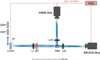Fig. 1 Schematic of POPO. The optics are composed of a liquid crystal variable retarder (LCVR) in front of the telescope focus (TF), three lenses (L1, L2a and L2b), a band-pass filter (BF; RC band), and a polarizing beam splitter (PBS). A half-wave plate (HWP) and a quarter-wave plate (QWP) are inserted in front of the LCVR for Stokes $\hat{u}$ and $\hat{v}$ observations, respectively. Images are taken by an EM-CCD camera (ANDOR iXon) and a CMOS camera (ANDOR Zyla). A data acquisition device (DAQ) sends synchronized pulses to the LCVR and the two cameras.

3 Observations

POPO was mounted on the Cassegrain focus of the 2.0-m Nayuta telescope at the Nishi-Harima Astronomical Observatory, University of Hyogo. The test observations were conducted from November 2024 to April 2025. To evaluate the performance of POPO, we observed the bright (<10 mag) polarimetric standard stars listed in Schmidt et al. (1992). In addition, time-series polarimetry of asteroid (4) Vesta was conducted. While imaging polarimetry for extended sources is one of POPO’s major advantages, we first demonstrate its performance in point-source observations as part of the complete evaluation. Notably, imaging functionality is beneficial even in point-source observations because it enables subtraction of sky-background flux measured in the vicinity of a target image.

Except for some calibration observations, all the observations presented in this study were performed at a frame rate of 200 fps. Although the sensors of iXon and Zyla cover fields-of-view (FOVs) of ~1.2′ and ~2′, respectively, FOVs for point source polarimetry are limited to ~20″ by reading out only the region-of-interest (ROI). We applied 4 × 4 and 8 × 8 binning for iXon and Zyla, respectively, unless the object was extremely bright (≲3 mag). If the target was very bright and the pixel values can be saturated, a smaller binning size was applied. Small FOVs and a binning setting were adopted to achieve a high frame rate and reduce the data size. Examples of the images obtained are shown in Fig. 2.

Typically, a single ‘take’ of observations spans 150 s and acquires 30 000 frames (per camera), which are stored in a single FITS file. The EM gain of the iXon camera was increased up to ×100, enhancing the peak count of a stellar image to more than several thousand analog-to-digital units (ADU). The EM procedure reduces the contribution of readout noise by multiplying the signal electrons. All observations were conducted using an R_C-band filter. In most cases, we repeated a sequence consisting of one take of $\hat{q}$, one take of $\hat{u}$, and one take of $\hat{v}$.

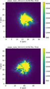Fig. 2 Images of β Cas observed on Nov. 13, 2024 with iXon (upper) and Zyla (lower). Each image corresponds to a single frame in a series acquired at 200 fps. The scale of a binned pixel is ~0.6″ for iXon and ~0.2″ for Zyla, with 4 × 4 binning applied to both cameras. The complex shapes of the stellar images are attributed to atmospheric turbulence.

4 Data reduction

Images were processed using a standard method. Dark frames were taken nightly. The camera configurations, such as the frame rate, ROI, and binning, were set to be identical to those of the object frames. The counts averaged over all dark frames were subtracted from the object frames.

Flat frames were obtained by pointing the telescope at a screen on the enclosure wall. The screen was illuminated using lamps attached to the top ring of the telescope. Because the lamps were not sufficiently bright for observations at 200 fps, flat frames were acquired at 2 fps. The instrumental configurations such as ROI, pixel binning, and Stokes mode ($\hat{q},\hat{u}$, or $\hat{v}$) were set to be identical to the object frames. To minimize the effects of the polarization of the light source, we averaged flat frames captured with symmetrically distributed ρ angles. We prepared a specific flat frame for each of the two LCVR retardance states (zero- and half-wavelength). In a series of frames stored in a single FITS file, even- and odd-numbered frames correspond to different states of the LCVR; thus, specifically prepared flat frames were applied. A common set of master flat frames was used for all object frames presented in this study.

Aperture photometry was performed on dark-subtracted and flat-fielded frames as follows. (i) All frames included in the FITS file are combined into a single frame. (ii) We ran the source extraction program SEP² (Barbary 2016) on the combined frame to determine the central position and size of the stellar image. These results, derived from the combined frame, were then used to define the position and radius of the circular aperture for photometry. The fixed aperture configuration was applied to all uncombined frames contained in the FITS file. (iii) Aperture photometry was performed using the Astropy package Photutils (Bradley et al. 2024). Sky background counts were measured in the annulus region around the circular aperture. Sky subtraction was performed separately for each frame.

The Stokes parameters can be derived using two methods. In the first method, which we refer to as the ‘single-ratio method’, the value of the Stokes parameter is derived from two photometric counts from two consecutive frames captured using a single camera. For $\hat{q}$-mode observations with iXon, we have $${\hat{q}}_{\mathrm{i}\mathrm{x}\mathrm{o}\mathrm{n}}=\frac{X(2j)-X(2j+1)}{X(2j)+X(2j+1)},$$(1)

where X(j) denotes the photometric count of an object in the jth (numbered based on a zero-based approach) frame in a FITS file captured with iXon. Similarly, for the Zyla data, $${\hat{q}}_{\mathrm{z}\mathrm{y}\mathrm{l}\mathrm{a}}=-\frac{Z(2j)-Z(2j+1)}{Z(2j)+Z(2j+1)},$$(2)

where Z(j) is the same as X(j) except the data are from Zyla.

In the second method, referred to as the ‘double-ratio method’, the Stokes value is calculated using data from both cameras: $$R=\sqrt{\frac{Z(2j)}{X(2j)}\frac{X(2j+1)}{Z(2j+1)}},$$(3) $${\hat{q}}_{\text{double\hspace{0.17em}}}=\frac{1-R}{1+R}.$$(4)

We attempted to use both the methods and compared their results (Section 5.1).

When an observation is conducted in the $\hat{u}$ mode, the same Equations (1)–(4) yield $\hat{u}$. This is similar to the case of the $\hat{v}$ mode; however, the signs are inverted to maintain consistency with Angel et al. (1972) and West (1989)³. We have $${\hat{v}}_{\text{ixon\hspace{0.17em}}}=-\frac{X(2j)-X(2j+1)}{X(2j)+X(2j+1)},$$(5) $${\hat{v}}_{\text{zyla\hspace{0.17em}}}=\frac{Z(2j)-Z(2j+1)}{Z(2j)+Z(2j+1)},$$(6) $${\hat{v}}_{\text{double\hspace{0.17em}}}=-\frac{1-R}{1+R},$$(7)

where R is the same as Eq. (3).

5 System characteristics and performance

5.1 Precision

Figure 3 shows the result from a single take (30 000 frames of continuous observations) of a bright unpolarized star, β Cas (1.97 mag in R_C, Ducati 2002)⁴. The left and right panels display $\hat{q}$ values derived using the single-ratio and double-ratio methods, respectively. Evidently, the scatter of $\hat{q}$ is much smaller in the double-ratio method than in the single-ratio method.

Table 1 summarizes the statistical measures of the single- and double-ratio methods. The one-take standard errors (ϵ) obtained using the single-ratio method are larger than those obtained using the double-ratio method by a factor of ~5. Although the double-ratio method utilizes approximately double the number of photons compared with the single-ratio method, the precision improvement by this effect should be a factor of only $\sim \sqrt{2}$. The much larger improvement (factor of ~5) indicates that the scatter of $\hat{q}$ derived using the single-ratio method (shown in Fig. 3, left) was caused not only by photon noise. Presumably, atmospheric disturbance is still in effect in the single-ratio method, despite the fast modulation of 200 Hz. In contrast, the double-ratio method suppresses the disturbance effect by taking Z(j)/X(j) (see Eq. (3)), which is the ratio of two photometric counts measured almost simultaneously.

In Fig. 4, ϵ values of $\hat{q},\hat{u}$ and $\hat{v}$ for ten different stars (~2–9 mag) are plotted against the number of detected photo-electrons, N_e. We converted the photometric counts (in ADU) into N_e by using the conversion factors (in e⁻/ADU) presented in the performance sheets of the cameras. When the EM was enabled for iXon, we estimated the number of electrons before multiplication based on the applied EM gain⁵.

As is shown in Fig. 4, we achieved a minimum ϵ of ~5 ppm (~5 × 10⁻⁶) when ~2 × 10¹¹ photo-electrons were detected, and the double-ratio method was used. The smallest ϵ (regardless of the method) for a certain N_e reached 2.5× the photon noise limit, or even below. The achievable ϵ under good conditions can be approximated as $$ϵ\approx 2.5/\sqrt{N_{\mathrm{e}}}.$$(8)

Figure 4 demonstrates that the ϵ obtained using the double-ratio method is significantly smaller than that obtained using the single-ratio method in the region of N_e ≳ 10¹⁰. However, in the region N_e ≲ 10⁹, ϵ extracted from the iXon-only measurements (single-ratio method) tends to be smaller than that derived from the double-ratio method. We note that iXon-only ϵ is significantly smaller than Zyla-only ϵ when the photon rate is low. This can be attributed to the benefits of EM, which only iXon is capable of. The advantage of the double-ratio method (as discussed above) is probably overwhelmed by the disadvantage of including lower-quality Zyla data when the photon rate is so small that the contribution of readout noise is significant. We expect a smaller ϵ, particularly in the region N_e ≲ 10⁹, if Zyla is replaced by iXon in the future (i.e., two iXon cameras are used).

The N_e value should be proportional to the integration time (Δt)⁶ and the stellar flux as long as the telluric transmittance is constant. This relationship is expressed as follows: $$N_{\mathrm{e}}=k\cdot \mathrm{\Delta }t\cdot {10}^{-m/2.5}\text{,\hspace{0.17em}}$$(9)

where k is the proportionality constant and m is the R_C-band magnitude of the star. We determined k for both iXon and Zyla as shown in Fig. 5. We have k = k_ixon + k_zyla = 5.6 × 10⁹ when Δt is expressed in seconds.

Combining Eqs. (8) and (9), we obtain the relationship among ϵ, Δt, and m as follows: $$ϵ\approx \frac{2.5}{\sqrt{k\cdot \mathrm{\Delta }t\cdot {10}^{-m/2.5}}}$$(10)

This equation is useful for planning observations. For reference, ϵ was calculated for Δt = 150 s (the typical time span of one take) and Δt = 1 s as shown in Fig. 6. Even for observations with a very high time resolution of Δt = 1 s, we expect ϵ < 1% for objects with m < 10 mag.

The one-take standard errors (ϵ) presented in this subsection should be interpreted as the achievable precision under nearly constant conditions, including atmospheric factors, ρ angles, and other relevant parameters. In Section 5.5, we evaluated the night-to-night stability or precision that can be achieved over different nights when the observational conditions may vary. In the following section, we focus on the system characteristics and performance based on measurements using the double-ratio method.

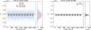Fig. 3 $\hat{q}$ values derived from one take (30 000 frames of observations) of β Cas on Nov. 13, 2024. Left: results from the single-ratio method, where blue plots are from Zyla and pink/red plots are from iXon. Right: results from the double-ratio method. The horizontal axis of each panel is equivalent to a time domain spanning 150 s. The smaller dots represent all measurements (15 000 values). The larger plots (connected by lines) are results after the original values are divided into ten bins. The histograms are displayed on the right side, with colors matching those of the scatter plots.

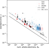Fig. 4 Standard errors (ϵ) of $\hat{q},\hat{u}$, and $\hat{v}$ measured for different standard stars plotted against numbers of detected photo-electrons (Ne). Blue triangles represent measurements using the Zyla data only (single-ratio method). Red circles are the same as the blue triangles except they are using the iXon data. Black squares denote measurements using the double-ratio method. A single symbol is from one take. In most cases, one take consists of 30 000 frames (Δt = 150 s). All the observations were conducted with 200 fps. The size of the red circles and the black squares represents the EM gain applied to iXon observations; the smallest and largest symbols correspond to gain factors of ×1 (no gain) and ×100, respectively. The solid line displays the photon noise limit, which is $ϵ=1/\sqrt{N_{\mathrm{e}}}$. The dashed line is 2.5 times the limit.

5.2 Artificial polarization

For accurate measurements, the relationship between the true values (${\hat{q}}_{\text{true}},{\hat{u}}_{\text{true}},{\hat{v}}_{\text{true}}$) and observed raw values (${\hat{q}}_{\text{raw}},{\hat{u}}_{\text{raw}},{\hat{v}}_{\text{raw}}$) should be determined. The raw values are the averages of all values derived from a single take using the double-ratio method (Eq. (4) for $\hat{q}$). We assumed the following linear relationship: $$\left(\begin{array}{l}{\hat{q}}_{\text{raw\hspace{0.17em}}}\\ {\hat{u}}_{\text{raw\hspace{0.17em}}}\\ {\hat{v}}_{\text{raw\hspace{0.17em}}}\end{array}\right)=M\left(\begin{array}{l}{\hat{q}}_{\text{true\hspace{0.17em}}}\\ {\hat{u}}_{\text{true\hspace{0.17em}}}\\ {\hat{v}}_{\text{true\hspace{0.17em}}}\end{array}\right)+\left(\begin{array}{l}\mathrm{\Delta }\hat{q}\\ \mathrm{\Delta }\hat{u}\\ \mathrm{\Delta }\hat{v}\end{array}\right),$$(11)

where M is a 3 × 3 matrix, which we refer to as the response matrix, and ($\mathrm{\Delta }\hat{q},\mathrm{\Delta }\hat{u},\mathrm{\Delta }\hat{v}$) is the artificial polarization generated in the observation system (Nayuta telescope and POPO).

By observing unpolarized stars (${\hat{q}}_{\text{true}}={\hat{u}}_{\text{true}}={\hat{v}}_{\text{true}}=0$), we can obtain the artificial polarization ($\mathrm{\Delta }\hat{q},\mathrm{\Delta }\hat{u},\mathrm{\Delta }\hat{v}$) directly from the raw values (${\hat{q}}_{\text{raw}},{\hat{u}}_{\text{raw}},{\hat{v}}_{\text{raw}}$). Thus, we observed β Cas, γ Gem, θ UMa, and ζ Peg, which are listed as unpolarized standard stars (hereafter, UP stars) in Schmidt et al. (1992). The observations were conducted between November 2024 and February 2025.

Figure 7 displays the raw Stokes values of the UP stars, which can be regarded as artificial polarization. We found that $\mathrm{\Delta }\hat{q},\mathrm{\Delta }\hat{u}$, and $\mathrm{\Delta }\hat{v}$ depend on the angle of the instrumental rotator ρ. The sine functions fitted the observations well. The functions are in the form of $$\mathrm{\Delta }\hat{s}=a+b\sin (2\rho +c),$$(12)

where $\hat{s}$ denotes $\hat{q},\hat{u}$ or $\hat{v}$. The best-fit parameters a, b, and c are listed in Table 2. The behavior of $\mathrm{\Delta }\hat{q}$ and $\mathrm{\Delta }\hat{u}$ shows that the degree of artificial LP is ~0.2% and that its position angle, as defined in the instrumental coordinate, changes as POPO rotates relative to the telescope. This indicates that artificial polarization is generated primarily in the telescope, not in POPO. If the polarization in POPO were dominant, it would not depend on ρ. It is natural to interpret the apparent dependence of $\mathrm{\Delta }\hat{v}$ on ρ as a result of the LP-to-CP crosstalk ($\hat{q}\to \hat{v}$ and $\hat{u}\to \hat{v}$), because the degree of CP does not depend on the observer’s position angle.

The differences between the observed ${\hat{s}}_{\text{raw}}$ and the predicted $\mathrm{\Delta }\hat{s}$ (Eq. (12)) are shown in the lower panel of Fig. 7. The root-mean-square (RMS) value of the residuals was ~60–70 ppm. These values were larger than the typical standard error of a single data point (~10 ppm). Smaller RMS values (a few tens of ppm) were obtained when the sine function was fitted to the data points of a single star observed on a single night. This implies that the profile (parameters a, b, and c) of artificial polarization varies from night to night and/or that the individual UP standard stars have polarization to a measurable degree. This also suggests that a UP star should be observed on the same night as the target observation if an accuracy or night-to-night stability of better than 100 ppm is required. We followed this strategy in evaluating the night-to-night stability (see Section 5.5). The parameters listed in Table 2 should be regarded as typical values during the test observation period.

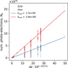Fig. 5 Relationship among Ne, Δt, and m. Blue triangles and red circles represent the data captured with Zyla and iXon, respectively. The lines fitted using Eq. (9) are drawn separately for the Zyla and iXon data. The data points at a certain x (= Δt · 10−m/2.5) exhibit a vertical scatter depending on the atmospheric clearness. To avoid underestimating k, the fitting was performed considering Ne/x as weights. The lower k for Zyla than iXon is presumably owing to the shorter effective exposure time of Zyla (~3.4 ms for Zyala vs ~4.8 ms for iXon) and the lower quantum efficiency of Zyla (~80% for Zyla vs ~95% for iXon at the wavelength of ~650 nm).

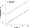Fig. 6 Relationship between ϵ and m for for Δt = 150 s (the solid line) and Δt = 1 s (the dashed line), as calculated by Eq. (10).

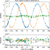Fig. 7 Observations of UP stars. Upper: raw Stokes values plotted against angles of the instrumental rotator (ρ). Blue circles, orange triangles, and green squares represent ${\hat{q}}_{\text{raw}},{\hat{u}}_{\text{raw}}$, and ${\hat{v}}_{\text{raw}}$, respectively. Fit curves in the form of Eq. (12) are also displayed. The data points shown as open plots are excluded from the fitting. The parameters of the fit curves are summarized in Table 2. Lower: differences between the raw Stokes values and the fit curves. The RMS values are written at a corner.

5.3 Instrumental response

In principle, M in Eq. (11) can be derived by measuring the Stokes parameters of several strongly polarized stars whose ${\hat{q}}_{\text{true}}$, ${\hat{u}}_{\text{true}}$, and ${\hat{v}}_{\text{true}}$ are known. In reality, stars with significant and stable CP are rarely identified. As far as we know, the white dwarf Grw +70° 8247 is the only object used as a CP standard star (Butters et al. 2009) due to its strong and stable CP (|v| ~ 2–4%; Kemp et al. 1970; Angel & Landstreet 1970; Angel et al. 1972; West 1989; Bagnulo & Landstreet 2019). Unfortunately, it is too faint (13.5 mag, Monet et al. 2003) to be observed at 200 fps with the Nayuta/POPO system. Because the polarimetric efficiencies (i.e., diagonal elements of M) depend on the ratio of the LCVR transition time to the frame time, as described in Appendix A, we cannot derive M for 200 fps directly from data taken at a slower frame rate. Therefore, determining M as a full 3×3 matrix is not feasible.

Nonetheless, most stars have a much weaker CP than LP. In this case, the terms containing v_true in Eq. (11) can be neglected (we discuss adequacy of the neglect at the end of this subsection). Thus, Eq. (11) reduces to $$\left(\begin{array}{l}{\hat{q}}_1\\ {\hat{u}}_1\\ {\hat{v}}_1\end{array}\right)\equiv \left(\begin{array}{l}{\hat{q}}_{\text{raw\hspace{0.17em}}}-\mathrm{\Delta }\hat{q}\\ {\hat{u}}_{\text{raw\hspace{0.17em}}}-\mathrm{\Delta }\hat{u}\\ {\hat{v}}_{\text{raw\hspace{0.17em}}}-\mathrm{\Delta }\hat{v}\end{array}\right)=M^{\mathrm{\prime }}(\genfrac{}{}{0ex}{}{{\hat{q}}_{\text{true\hspace{0.17em}}}}{{\hat{u}}_{\text{true\hspace{0.17em}}}}),$$(13)

where M′ denotes the partial (3×2) response matrix (the first two columns of the original M). In this equation, ${\hat{s}}_1$ is the measured Stokes value after subtracting the artificial polarization ($\mathrm{\Delta }\hat{s}$). The value of $\mathrm{\Delta }\hat{s}$ is calculated using Eq. (12) for ρ at the observation.

To obtain M′, we observed four stars with strong LP (hereafter, LP stars), which are listed as polarized standard stars in Schmidt et al. (1992). They have degrees of LP ranging ~4–6% and a brightness of ~5–9 mag. We observed an LP star with several different ϕ angles (position angles of the FOV) whenever time permitted. This yields multiple (${\hat{q}}_{\text{true}},{\hat{u}}_{\text{true}}$) points (star-shaped marks in Fig. 8) on the $\hat{q}\text{-}\hat{u}$ plane⁷ from a single star.

The observational results are plotted on the $\hat{q}-\hat{u}$ plane in Fig. 8 (left). The notable discrepancies between (${\hat{q}}_1,{\hat{u}}_1$) and (${\hat{q}}_{\text{true}},{\hat{u}}_{\text{true}}$) should be corrected.

Using the least-squares method, M′ was calculated as $$M^{\mathrm{\prime }}=\left(\begin{array}{cc}0.803\pm 0.008& -0.161\pm 0.008\\ -0.045\pm 0.007& 0.811\pm 0.007\\ 0.050\pm 0.009& -0.011\pm 0.010\end{array}\right).$$(14)

The (j, j) elements (diagonal elements in the original M) signify the polarimetric efficiencies, which should be 100% for an ideal instrument. For POPO, these values were ~80%. This implies that ~20% of $\hat{q}$ and $\hat{u}$ are lost. The other elements describe factors of crosstalk effect, which should ideally be zero. For POPO, they typically marked several percent, except for the (0, 1) element (~16%), specifying the $\hat{u}\to \hat{q}$ crosstalk.

Here, we discuss the impact of neglecting the third column of the original M. From the first row of Eq. (11), we can write the ratio of the systematic alteration ($\delta \hat{q}\equiv {\hat{q}}_1-{\hat{q}}_{\text{true}}$) to the true value as $$\frac{\delta \hat{q}}{{\hat{q}}_{\text{true\hspace{0.17em}}}}=-(1-m_{11})+m_{12}\frac{{\hat{u}}_{\text{true\hspace{0.17em}}}}{{\hat{q}}_{\text{true\hspace{0.17em}}}}+m_{13}\frac{{\hat{v}}_{\text{true\hspace{0.17em}}}}{{\hat{q}}_{\text{true\hspace{0.17em}}}},$$(15)

where m_ij denotes the (i, j) element of M. We assume that m₁₃, representing the factor of $\hat{v}\to \hat{q}$ crosstalk, has a similar value to the other crosstalk factors presented in Eq. (14). In the case where CP is an order of magnitude weaker than LP, i.e., ${\hat{q}}_{\text{true}}\sim {\hat{u}}_{\text{true}}\sim 10{\hat{v}}_{\text{true}}$, the third term of Eq. (15) (involving ${\hat{v}}_{\text{true}}$) is on the order of 10⁻², which is significantly smaller than the first two terms, both of which are on the order of 10⁻¹. In the case where CP is as strong as LP (${\hat{q}}_{\text{true}}\sim {\hat{u}}_{\text{true}}\sim {\hat{v}}_{\text{true}}$), all three terms are on the order of 10⁻¹. A similar discussion applies to $\hat{u}$ based on the second row of Eq. (11).

Adequacy of neglecting the terms containing ${\hat{v}}_{\text{true}}$ depends on both the required level of accuracy and the CP-to-LP ratio of the source. When a relative accuracy of 10⁻¹ with respect to ${\hat{q}}_{\text{true}}$ is required for a source satisfying ${\hat{q}}_{\text{true}}\sim 10{\hat{v}}_{\text{true}}$, neglecting the ${\hat{v}}_{\text{true}}$-dependent terms is justified. However, if a higher accuracy is required – for example, a relative accuracy of 10⁻² – omitting the ${\hat{v}}_{\text{true}}$-dependent terms may lead to significant systematic error.

Obviously, a full 3 × 3 formulation of M is anticipated. One possible approach to estimating the third column of M for 200 fps is to derive M at slower frame rates and evaluate the dependence of M on frame rate. We leave this investigation for future work.

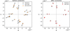Fig. 8 Observed ($\hat{q},\hat{u}$) before correction (left) and after correction (right) in comparison with values in the literature (Schmidt et al. 1992). Blue triangles, orange squares, and red circles represent raw Stokes (${\hat{q}}_{\text{raw}},{\hat{u}}_{\text{raw}}$), Stokes after subtraction of artificial polarization (${\hat{q}}_1,{\hat{u}}_1$), and response-corrected Stokes $({\hat{q}}_2,{\hat{u}}_2)$, respectively. The star-shaped plots are from the literature.

5.4 Accuracy

Once we obtain partial response matrix M′, we can correct (${\hat{q}}_1,{\hat{u}}_1$) by $$(\genfrac{}{}{0ex}{}{{\hat{q}}_2}{{\hat{u}}_2})=M_{qu}^{-1}(\genfrac{}{}{0ex}{}{{\hat{q}}_1}{{\hat{u}}_1}),$$(16)

where M_qu denotes the first two rows of M′⁸; Its inverse matrix was determined to be $$M_{qu}^{-1}=\left(\begin{array}{ll}1.260\pm 0.012& 0.250\pm 0.013\\ 0.071\pm 0.010& 1.246\pm 0.011\end{array}\right).$$(17)

The corrected values (${\hat{q}}_2,{\hat{u}}_2$) are shown in Fig. 8 (right). The discrepancies between the observations and literature have been greatly diminished.

The equatorial Stokes (q, u) was obtained by rotating a vector pointing (${\hat{q}}_2,{\hat{u}}_2$) by +2ϕ on the $\hat{q}-\hat{u}$ plane. The degree (P) and position angle (θ) of the LP were derived as $$P=\sqrt{q^2+u^2},$$(18) $$\tan 2\theta =\frac{u}{q},\text{\hspace{0.17em}and\hspace{0.17em}}\mathrm{sgn}(\cos 2\theta )=\mathrm{sgn}(q),$$(19)

where sgn(x) stands for ‘sign of x’ (Hovenier et al. 2004).

In Table 3, the observed P and θ values are compared with those in the literature (Schmidt et al. 1992). The discrepancies in P were ≲0.1% when observations included the full set of ϕ angles (0°, 45°, 90°, and 135°), while they were ~0.3% when only one or two ϕ angles were used. Discrepancies in θ was ≲1.5°.

We note the possibility that some of the standard stars used in our analysis may be variable. Breus et al. (2021) reported suspected variability for BD+59 389 (HD 236928), HD 154445, HD 204827, and HD 25443. The measured P of HD 204827 in Schmidt et al. (1992) is consistent with that in Bailey & Hough (1982), but shows a significant deviation from the value reported in Hsu & Breger (1982). Errors in the reference values can introduce systematic errors in the response matrix. We plan to monitor these stars to investigate their variability and to validate our accuracy assessment.

5.5 Night-to-night stability

To assess the night-to-night stability of the measurement, we observed θ UMa (2.74 mag, Ducati 2002) on three nights in March 2025. The sequence of ($\hat{q},\hat{u},\hat{v}$) observations was repeated to 5–8 times per night. The ϕ angle was fixed to 0° (North is up in the FOV) using an instrumental rotator; thus, the ρ angle varied with time. We also observed β UMa (2.31 mag, Ducati 2002) at several ρ angles every night to determine artificial polarization $\mathrm{\Delta }\hat{s}$ as a function of ρ (Eq. (12)). Both θ UMa (target) and β UMa (reference) are listed as UP stars in Schmidt et al. (1992).

Artificial polarization $\mathrm{\Delta }\hat{s}$ was determined nightly in the form of Eq. (12) from reference observations. Then, $\mathrm{\Delta }\hat{s}$ was subtracted from the raw values of the target. The upper panel of Fig. 9 shows the subtracted values, ${\hat{s}}_1(={\hat{s}}_{\text{raw\hspace{0.17em}}}-\mathrm{\Delta }\hat{s})$, on three nights. If artificial polarization were completely removed, ${\hat{s}}_1$ would not show any dependence on the ρ angle. However, a 180° periodic dependence on ρ remains recognizable. One possible explanation is that the artificial polarization depends on stellar spectral type: the spectral types of θ UMa and β UMa are F 7 V (Abt 2009) and A1IVps (Phillips et al. 2010), respectively. In general, telescope polarization and the retardance of waveplates, including LCVRs, are known to have dependence on wavelength. This raises the possibility that broadband artificial polarization differs between stars of different spectral types. This scenario will be explored in subsequent studies.

Although the underlying mechanism remains elusive, the dependence on ρ cannot be astrophysical; it must be artificial. Thus, we fitted a function in the same form as Eq. (12) to ${\hat{s}}_1$ (Fig. 9, upper panel), and subtracted the sine component b′ sin(2ρ + c′) from ${\hat{s}}_1$. The Stokes values after the second subtraction are denoted by ${\hat{s}}_{1\mathrm{b}}$ and displayed in the lower panel of Fig. 9. The ρ dependence was largely removed.

We corrected ${\hat{q}}_{1\mathrm{b}}$ and ${\hat{u}}_{1\mathrm{b}}$ using M_qu⁻¹ (similar to Eq. (16)), which yields final q and u⁹. We treated ${\hat{v}}_{1\mathrm{b}}$ as v. The results are summarized in Table 4. The night-to-night stability, defined as standard deviation of the nightly averages, was ≲10 ppm for q, u, and v.

5.6 Demonstration

Finally, we demonstrate the capability of POPO for scientific observations. Asteroid (4) Vesta is known to exhibit rotational variation in the LP (Degewij et al. 1979; Broglia & Manara 1989; Lupishko et al. 1999; Wiktorowicz & Nofi 2015; Cellino et al. 2016). To confirm the rotational variation, we conducted time-series polarimetry of Vesta on three nights in April 2025. The observations spanned approximately 4–6 h per night, covering (almost) the full rotation period of Vesta (~5.3 h, Park et al. 2025)¹⁰. During our observations, the magnitude of Vesta was ~6 mag, and the Sun–Vesta–Earth phase angle (α) was ~10°−14°¹¹. A UP star, β UMa, was observed nightly to obtain the artificial polarization profile for that particular night. The Stokes parameters were derived using the same procedure described in Section 5.5 except that the longer time span of Vesta observations per night allowed us to perform the second subtraction of the artificial polarization separately each night.

The observed P values of Vesta are shown in Fig. 10. The nightly averages $\overline{P}$ were ~0.5% to ~0.6%, which is in agreement with previous observations (archived in Lupishko 2022, summarized in Bach et al. 2024). The rotational variation in P was clearly detected for all three epochs. The peak-to-peak variations ΔP were ~0.06%-0.08%. The $\mathrm{\Delta }P/\overline{P}$ ratios were ~0.12–0.16, consistent with previous reports of $\mathrm{\Delta }P/\overline{P}\approx 0.06-0.22$ (Wiktorowicz & Nofi 2015; Cellino et al. 2016). The detection confidence, defined as the ratio of ΔP to the typical error of P, was ~60 for all three nights. The confidence appears as strong as that of the 1978 and 1986 data presented in Figure 11 of Cellino et al. (2016), based on our visual inspection. To the best of our knowledge, our dataset is among the most reliable in terms of confidence and reproducibility for observations of Vesta’s rotational LP variation. This experiment demonstrates the high capability of POPO for precision polarimetry.

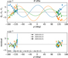Fig. 9 Observed Stokes values of θ UMa. Upper: Stokes values after subtraction of the artificial polarization. The colors represent each of Stokes: ${\hat{q}}_1$ (blue), ${\hat{u}}_1$ (orange), and ${\hat{v}}_1$ (green). The shapes of the plots correspond to observation dates as explained in the lower panel. Fit curves in the form of Eq. (12) are also drawn. Lower: differences between the observed values $({\hat{q}}_1,{\hat{u}}_1,{\hat{v}}_1)$ and the fit curves.

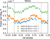Fig. 10 Observed P of Vesta. In the legends, α represents Sun–Vesta–Earth phase angle. The data values are exhibited in Table B.1.

6 Conclusions

We developed POPO and evaluated its performance on bright (<10 mag) point sources. The key performance metrics are summarized as follows:

• Precision of Stokes measurement under nearly constant conditions reached 2.5 times the photon noise limit and marked 5 ppm at best (Section 5.1);

• Even with a time resolution of 1 s, a precision less than 1% is expected for a 10-mag source (Section 5.1);

• Night-to-night stability was recorded to be ≲10 ppm (Section 5.5);

• Accuracy of P for strongly polarized stars (P ≈ several %) was evaluated to be ≲0.1% when observations included all four ϕ angles (0°, 45°, 90°, and 135°) (Section 5.4).

POPO is well suited for studying small polarimetric variations in bright objects, as demonstrated by our observations of Vesta (Section 5.6). In addition, it has been shown that POPO has capability of high-time-resolution polarimetry (Section 5.1).

Although we focused on point-source observations in this study, POPO has the potential for spatially resolved polarimetry for extended sources owing to its imaging capability. Further performance evaluations are planned for the near future.

Acknowledgements

We are grateful to Jeremy Bailey for his kind advice at the early stage of this study. We sincerely appreciate Masateru Ishiguro for his invaluable comments on our Vesta observations. Furthermore, we acknowledge Hiroyuki Maehara for his contributions to the exploration of science cases for POPO. This study was supported by Tokubetsu Kenkyu Joseikin (2019–2021) from University of Hyogo; Sumitomo Foundation Grant for Basic Science Research Projects (No. 191076); NAOJ Research Coordination Committee, NINS (NAOJ-RCC-2101-0106); Academic Research Grant from the Hyogo Science and Technology Association (HyogoSTA); Japan Society for the Promotion of Science (JSPS) KAKENHI Grant Number 21 K 036481; and the Optical and Infrared Synergetic Telescopes for Education and Research (OISTER) program funded by the MEXT of Japan. This study utilized the Python package Uncertainties (Eric O. Lebigot, http://pythonhosted.org/uncertainties/) for handling calculations with uncertainties.

References

Appendix A Laboratory experiment of LCVR

Before assembling POPO, we tested the polarization modulation by LCVR in our laboratory. Figure A.1 shows the experimental setup and results. When a high voltage (V_high) is applied to the LC cell, it provides virtually no retardance (0λ). At a lower voltage (V_low), it produces a retardance of half a wavelength (λ/2). If λ/2-retardance is given, the position angle of the incident LP rotates.

Polarization modulation was visualized as a light curve (Fig. A.1, right). The ‘plateaus’ with a higher signal level in the light curves correspond to the 0λ (V_high) state of LCVR, whereas the ‘valleys’ with a lower signal level represent the λ/2 (V_low) state.

As shown in Fig. A.1 (right), the transition from the 0λ state to the λ/2 state requires ~2 ms. This restricts the applicability of the modulation frequencies. We selected 200 Hz for the normal operation because it is the fastest applicable frequency. Notably, the apparent depolarization in the measurements with POPO can be attributed to the nonzero transition time. A single image frame is acquired during a single state (a single plateau or valley spanning 5 ms), and the signals within the state are integrated. This causes the measured plateau–valley contrast to be lower than the true value. The apparent depolarization increases with the ratio of the transition time to the duration of a single frame (5 ms in the 200 fps case).

In the current operation of POPO, we set V_high = 11.5 V and V_low = 1.76 V to minimize the $\hat{q}\to \hat{v}$ crosstalk in the R_C-band light. The difference between the actual retardance and desired retardance (0λ or λ/2) causes crosstalk.

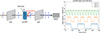Fig. A.1 Laboratory test of LCVR with different modulation frequencies. Left: Schematic of the setup. The LCVR is sandwiched by two polarizing filters whose transmitting axes are aligned. We used an RC-band filter, which does not appear here. Right: Measured light curves. Strength of light signals are output by a PMT (with an amplifier) as voltages. For a visibility reason, plots for 200 and 500 Hz are vertically offset.

Appendix B Results of the Vesta observations

Table B.1 presents the results of the Vesta observations, which are plotted in Fig. 10. The rotational phase was obtained using the rotation period 5.3421276322 ± 0.0000000004 h (Park et al. 2025).¹⁰ The time of the first observation (2025-04-06 14:57 UT) was set to be the origin of rotational phase. The observation time is the average of the start times of the q and u observations.

All Tables

All Figures

Fig. 1 Schematic of POPO. The optics are composed of a liquid crystal variable retarder (LCVR) in front of the telescope focus (TF), three lenses (L1, L2a and L2b), a band-pass filter (BF; RC band), and a polarizing beam splitter (PBS). A half-wave plate (HWP) and a quarter-wave plate (QWP) are inserted in front of the LCVR for Stokes $\hat{u}$ and $\hat{v}$ observations, respectively. Images are taken by an EM-CCD camera (ANDOR iXon) and a CMOS camera (ANDOR Zyla). A data acquisition device (DAQ) sends synchronized pulses to the LCVR and the two cameras.

In the text

	Fig. 2 Images of β Cas observed on Nov. 13, 2024 with iXon (upper) and Zyla (lower). Each image corresponds to a single frame in a series acquired at 200 fps. The scale of a binned pixel is ~0.6″ for iXon and ~0.2″ for Zyla, with 4 × 4 binning applied to both cameras. The complex shapes of the stellar images are attributed to atmospheric turbulence.
In the text

Fig. 3 $\hat{q}$ values derived from one take (30 000 frames of observations) of β Cas on Nov. 13, 2024. Left: results from the single-ratio method, where blue plots are from Zyla and pink/red plots are from iXon. Right: results from the double-ratio method. The horizontal axis of each panel is equivalent to a time domain spanning 150 s. The smaller dots represent all measurements (15 000 values). The larger plots (connected by lines) are results after the original values are divided into ten bins. The histograms are displayed on the right side, with colors matching those of the scatter plots.

In the text

Fig. 4 Standard errors (ϵ) of $\hat{q},\hat{u}$, and $\hat{v}$ measured for different standard stars plotted against numbers of detected photo-electrons (Ne). Blue triangles represent measurements using the Zyla data only (single-ratio method). Red circles are the same as the blue triangles except they are using the iXon data. Black squares denote measurements using the double-ratio method. A single symbol is from one take. In most cases, one take consists of 30 000 frames (Δt = 150 s). All the observations were conducted with 200 fps. The size of the red circles and the black squares represents the EM gain applied to iXon observations; the smallest and largest symbols correspond to gain factors of ×1 (no gain) and ×100, respectively. The solid line displays the photon noise limit, which is $ϵ=1/\sqrt{N_{\mathrm{e}}}$. The dashed line is 2.5 times the limit.

In the text

Fig. 5 Relationship among Ne, Δt, and m. Blue triangles and red circles represent the data captured with Zyla and iXon, respectively. The lines fitted using Eq. (9) are drawn separately for the Zyla and iXon data. The data points at a certain x (= Δt · 10−m/2.5) exhibit a vertical scatter depending on the atmospheric clearness. To avoid underestimating k, the fitting was performed considering Ne/x as weights. The lower k for Zyla than iXon is presumably owing to the shorter effective exposure time of Zyla (~3.4 ms for Zyala vs ~4.8 ms for iXon) and the lower quantum efficiency of Zyla (~80% for Zyla vs ~95% for iXon at the wavelength of ~650 nm).

In the text

	Fig. 6 Relationship between ϵ and m for for Δt = 150 s (the solid line) and Δt = 1 s (the dashed line), as calculated by Eq. (10).
In the text

Fig. 7 Observations of UP stars. Upper: raw Stokes values plotted against angles of the instrumental rotator (ρ). Blue circles, orange triangles, and green squares represent ${\hat{q}}_{\text{raw}},{\hat{u}}_{\text{raw}}$, and ${\hat{v}}_{\text{raw}}$, respectively. Fit curves in the form of Eq. (12) are also displayed. The data points shown as open plots are excluded from the fitting. The parameters of the fit curves are summarized in Table 2. Lower: differences between the raw Stokes values and the fit curves. The RMS values are written at a corner.

In the text

Fig. 8 Observed ($\hat{q},\hat{u}$) before correction (left) and after correction (right) in comparison with values in the literature (Schmidt et al. 1992). Blue triangles, orange squares, and red circles represent raw Stokes (${\hat{q}}_{\text{raw}},{\hat{u}}_{\text{raw}}$), Stokes after subtraction of artificial polarization (${\hat{q}}_1,{\hat{u}}_1$), and response-corrected Stokes $({\hat{q}}_2,{\hat{u}}_2)$, respectively. The star-shaped plots are from the literature.

In the text

Fig. 9 Observed Stokes values of θ UMa. Upper: Stokes values after subtraction of the artificial polarization. The colors represent each of Stokes: ${\hat{q}}_1$ (blue), ${\hat{u}}_1$ (orange), and ${\hat{v}}_1$ (green). The shapes of the plots correspond to observation dates as explained in the lower panel. Fit curves in the form of Eq. (12) are also drawn. Lower: differences between the observed values $({\hat{q}}_1,{\hat{u}}_1,{\hat{v}}_1)$ and the fit curves.

In the text

	Fig. 10 Observed P of Vesta. In the legends, α represents Sun–Vesta–Earth phase angle. The data values are exhibited in Table B.1.
In the text

Fig. A.1 Laboratory test of LCVR with different modulation frequencies. Left: Schematic of the setup. The LCVR is sandwiched by two polarizing filters whose transmitting axes are aligned. We used an RC-band filter, which does not appear here. Right: Measured light curves. Strength of light signals are output by a PMT (with an amplifier) as voltages. For a visibility reason, plots for 200 and 500 Hz are vertically offset.

In the text

References

- Abt, H. A. 2009, ApJS, 180, 117 [Google Scholar]
- Angel, J. R. P., & Landstreet, J. D. 1970, ApJ, 162, L61 [NASA ADS] [CrossRef] [Google Scholar]
- Angel, J. R. P., Landstreet, J. D., & Oke, J. B. 1972, ApJ, 171, L11 [Google Scholar]
- Bach, Y. P., Ishiguro, M., Takahashi, J., et al. 2024, A&A, 684, A81 [NASA ADS] [CrossRef] [EDP Sciences] [Google Scholar]
- Bagnulo, S., & Landstreet, J. D. 2019, MNRAS, 486, 4655 [CrossRef] [Google Scholar]
- Bagnulo, S., Landolfi, M., Landstreet, J. D., et al. 2009, PASP, 121, 993 [Google Scholar]
- Bailey, J., & Hough, J. H. 1982, PASP, 94, 618 [NASA ADS] [CrossRef] [Google Scholar]
- Bailey, J., Kedziora-Chudczer, L., Cotton, D. V., et al. 2015, MNRAS, 449, 3064 [NASA ADS] [CrossRef] [Google Scholar]
- Bailey, J., Cotton, D. V., & Kedziora-Chudczer, L. 2017, MNRAS, 465, 1601 [Google Scholar]
- Bailey, J., Kedziora-Chudczer, L., & Bott, K. 2018, MNRAS, 480, 1613 [NASA ADS] [CrossRef] [Google Scholar]
- Bailey, J., Cotton, D. V., Kedziora-Chudczer, L., De Horta, A., & Maybour, D. 2020, PASA, 37, e004 [NASA ADS] [CrossRef] [Google Scholar]
- Bailey, J., Bott, K., Cotton, D. V., et al. 2021, MNRAS, 502, 2331 [NASA ADS] [CrossRef] [Google Scholar]
- Barbary. 2016, J. Open Source Softw., 1, 58 [CrossRef] [Google Scholar]
- Bazzon, A., Schmid, H. M., & Gisler, D. 2013, A&A, 556, A117 [NASA ADS] [CrossRef] [EDP Sciences] [Google Scholar]
- Bertin, E., & Arnouts, S. 1996, A&AS, 117, 393 [NASA ADS] [CrossRef] [EDP Sciences] [Google Scholar]
- Bradley, L., Sipőcz, B., Robitaille, T., et al. 2024, astropy/photutils: 2.0.2 [Google Scholar]
- Breus, V., Kolesnikov, S. V., & Andronov, I. L. 2021, arXiv e-prints [arXiv:2112.12277] [Google Scholar]
- Broglia, P., & Manara, A. 1989, A&A, 214, 389 [Google Scholar]
- Butters, O. W., Katajainen, S., Norton, A. J., Lehto, H. J., & Piirola, V. 2009, A&A, 496, 891 [NASA ADS] [CrossRef] [EDP Sciences] [Google Scholar]
- Cellino, A., Ammannito, E., Magni, G., et al. 2016, MNRAS, 456, 248 [Google Scholar]
- Degewij, J., Tedesco, E. F., & Zellner, B. 1979, Icarus, 40, 364 [Google Scholar]
- Drilling, J. S., & Landolt, A. U. 2000, in Allen’s Astrophysical Quantities, ed. A. N. Cox, 381 [Google Scholar]
- Ducati, J. R. 2002, VizieR On-line Data Catalog: II/237 [Google Scholar]
- Hough, J. H., Lucas, P. W., Bailey, J. A., et al. 2006, PASP, 118, 1302 [Google Scholar]
- Hovenier, J. W., Van Der Mee, C., & Domke, H. 2004, Transfer of polarized light in planetary atmospheres: basic concepts and practical methods, 318 [Google Scholar]
- Hsu, J. C., & Breger, M. 1982, ApJ, 262, 732 [NASA ADS] [CrossRef] [Google Scholar]
- Kemp, J. C., Swedlund, J. B., Landstreet, J. D., & Angel, J. R. P. 1970, ApJ, 161, L77 [NASA ADS] [CrossRef] [Google Scholar]
- Lupishko, D. 2022, Asteroid Polametric Database (APD) Bundle V2.0, NASA Planetary Data System, urn:nasa:pds:asteroid_polarimetric_database::2.0 [Google Scholar]
- Lupishko, D. F., Efimov, Y. S., & Shakhovskoi, N. M. 1999, Sol. Syst. Res., 33, 45 [Google Scholar]
- Miles-Páez, P. A., Pallé, E., & Zapatero Osorio, M. R. 2014, A&A, 562, L5 [Google Scholar]
- Monet, D. G., Levine, S. E., Canzian, B., et al. 2003, AJ, 125, 984 [Google Scholar]
- Park, R. S., Ermakov, A. I., Konopliv, A. S., et al. 2025, Nat. Astron., 9, 824 [Google Scholar]
- Phillips, N. M., Greaves, J. S., Dent, W. R. F., et al. 2010, MNRAS, 403, 1089 [NASA ADS] [CrossRef] [Google Scholar]
- Schmidt, G. D., Elston, R., & Lupie, O. L. 1992, AJ, 104, 1563 [Google Scholar]
- Seager, S., Whitney, B. A., & Sasselov, D. D. 2000, ApJ, 540, 504 [NASA ADS] [CrossRef] [Google Scholar]
- Shearer, A., Kanbach, G., Slowikowska, A., et al. 2010, in Proceedings of High Time Resolution Astrophysics – The Era of Extremely Large Telescopes (HTRA-IV), May 5–7, 54 [Google Scholar]
- Sterzik, M. F., Bagnulo, S., & Palle, E. 2012, Nature, 483, 64 [NASA ADS] [CrossRef] [Google Scholar]
- Sterzik, M. F., Bagnulo, S., Stam, D. M., Emde, C., & Manev, M. 2019, A&A, 622, A41 [NASA ADS] [CrossRef] [EDP Sciences] [Google Scholar]
- Takahashi, J., Itoh, Y., Akitaya, H., et al. 2013, PASJ, 65, 38 [CrossRef] [Google Scholar]
- Takahashi, J., Itoh, Y., Matsuo, T., et al. 2021, A&A, 653, A99 [NASA ADS] [CrossRef] [EDP Sciences] [Google Scholar]
- Wenger, M., Ochsenbein, F., Egret, D., et al. 2000, A&AS, 143, 9 [NASA ADS] [CrossRef] [EDP Sciences] [Google Scholar]
- West, S. C. 1989, ApJ, 345, 511 [CrossRef] [Google Scholar]
- Wiktorowicz, S. J., & Matthews, K. 2008, PASP, 120, 1282 [Google Scholar]
- Wiktorowicz, S. J., & Nofi, L. A. 2015, ApJ, 800, L1 [NASA ADS] [CrossRef] [Google Scholar]
- Wiktorowicz, S. J., Słowikowska, A., Nofi, L. A., et al. 2023, ApJS, 264, 42 [NASA ADS] [CrossRef] [Google Scholar]
Actually, ![Mathematical equation: $\[\hat{v}\]$](/articles/aa/full_html/2025/11/aa55724-25/aa55724-25-eq128.png) is identical to v.
is identical to v.
SEP is a Python module based on Source Extractor (Bertin & Arnouts 1996).
The opposite convention exists (e.g., Bagnulo et al. 2009).
In this paper, the RC-band magnitudes of the stars were retrieved from SIMBAD (Wenger et al. 2000, https://simbad.u-strasbg.fr/simbad/). If the RC-band magnitude was not available, it was estimated using the V-band magnitude in SIMBAD and the V–R color presented in Drilling & Landolt (2000).
We found that the effective multiplication factor is ~0.8 × (commanded EM gain). The effectiveness was considered in estimating the number of electrons before multiplication.
Here, Δt is defined by (frame time) × (number of frames). To be more accurate, Δt is apparent integration time, because the effective exposure time per frame is less than the frame time. The frame time is 5 ms at 200 fps. The effective exposure time is estimated to be ~4.8 ms and ~3.4 ms for iXon and Zyla, respectively.
We note that the ![Mathematical equation: $\[\hat{q}-\hat{u}\]$](/articles/aa/full_html/2025/11/aa55724-25/aa55724-25-eq129.png) plane is defined using instrumental coordinates.
plane is defined using instrumental coordinates.
As POPO does not observe ![Mathematical equation: $\[\hat{q}\]$](/articles/aa/full_html/2025/11/aa55724-25/aa55724-25-eq130.png) and
and ![Mathematical equation: $\[\hat{u}\]$](/articles/aa/full_html/2025/11/aa55724-25/aa55724-25-eq131.png) simultaneously, we create a pair of consecutive observations of
simultaneously, we create a pair of consecutive observations of ![Mathematical equation: $\[\hat{q}\]$](/articles/aa/full_html/2025/11/aa55724-25/aa55724-25-eq132.png) and
and ![Mathematical equation: $\[\hat{u}\]$](/articles/aa/full_html/2025/11/aa55724-25/aa55724-25-eq133.png) . The difference in the observation times was approximately ~4 min in a typical configuration (200 fps × 30 000 frames).
. The difference in the observation times was approximately ~4 min in a typical configuration (200 fps × 30 000 frames).
The coordinates need not be converted because ϕ = 0° in this case.
The rotation period was retrieved from NASA JPL Small-Body Database Lookup (https://ssd.jpl.nasa.gov/tools/sbdb_lookup.html).
The magnitudes and phase angles were retrieved from NASA JPL Horizons System (https://ssd.jpl.nasa.gov/horizons/app.html).