| Issue |
A&A
Volume 703, November 2025
|
|
|---|---|---|
| Article Number | A172 | |
| Number of page(s) | 19 | |
| Section | Interstellar and circumstellar matter | |
| DOI | https://doi.org/10.1051/0004-6361/202555836 | |
| Published online | 13 November 2025 | |
CO adsorption sites on interstellar water ices explored with machine learning potentials
Binding energy distributions and snowline
1
Departamento de Físico-Química, Facultad de Ciencias Químicas, Universidad de Concepción,
Concepción,
Chile
2
Atomistic Simulations, Italian Institute of Technology,
16152
Genova,
Italy
3
Departamento de Astrofísica Molecular, Instituto de Física Fundamental (IFF-CSIC),
C/ Serrano 121,
28006
Madrid,
Spain
4
RIKEN Pioneering Research Institute,
2-1 Hirosawa,
Wako-shi,
Saitama
351-0198,
Japan
5
Institute for Theoretical Chemistry, University of Stuttgart,
Pfaffenwaldring 55,
70569
Stuttgart,
Germany
★ Corresponding authors: This email address is being protected from spambots. You need JavaScript enabled to view it.
; This email address is being protected from spambots. You need JavaScript enabled to view it.
Received:
5
June
2025
Accepted:
14
August
2025
Abstract
Context. Carbon monoxide (CO) is arguably the most important molecule for interstellar organic chemistry. Its binding to amorphous solid water (ASW) ice regulates both diffusion and desorption processes. Accurately characterizing the CO binding energy (BE) is essential for realistic astrochemical modeling.
Aims. We aim to derive a statistically robust and physically accurate distribution of CO BEs on ASW surfaces, and to evaluate its implications for laboratory temperature-programmed desorption experiments and interstellar chemistry, with a focus on protoplanetary disks.
Methods. We trained a machine-learned potential (MLP) on 8321 density functional theory (DFT) energies and gradients of CO interacting with water clusters of different sizes (22–60 water molecules). The DFT method was selected after extensive benchmarking. With this potential, we built realistic nonporous and porous ASW surfaces and computed a BE distribution. We used symmetry-adapted perturbation theory to rationalize the interactions of CO with the different binding sites.
Results. We find that both ASW morphologies yield similar Gaussian-like BE distributions, with mean values near 900 K. However, the nature of the binding interactions is rather different and is critically dependent on surface roughness and dangling OH bonds. Simulated temperature-programmed desorption (TPD) curves reproduce experimental trends across several coverage regimes. From an astrochemical point of view, the application of the full BE distribution has a dramatic influence on the CO distribution in protoplanetary disks, leading to a broader CO snowline region, improving predictions of CO gas-ice partitioning, and suggesting an equally broader distribution of organics in these objects.
Key words: astrochemistry / ISM: general / ISM: molecules
© The Authors 2025
 Open Access article, published by EDP Sciences, under the terms of the Creative Commons Attribution License (https://creativecommons.org/licenses/by/4.0), which permits unrestricted use, distribution, and reproduction in any medium, provided the original work is properly cited.
This article is published in open access under the Subscribe to Open model. This email address is being protected from spambots. You need JavaScript enabled to view it. to support open access publication.
1 Introduction
Interstellar surface chemistry plays a pivotal role in the formation of complex organic molecules (COMs) in space (Herbst & van Dishoeck 2009; Cuppen et al. 2017). The icy mantles of dust grains provide a reactive environment in which atoms and molecules can accrete, diffuse, and interact, facilitating the synthesis of new species and driving molecular complexity in the interstellar medium (ISM). Within these surface-driven networks, certain molecules act as key nodes, either as chemically stable reservoirs (e.g., CH4, CO2, and N2) or as reactive intermediates that enable further chemical evolution. Among the latter, carbon monoxide (CO) is particularly important (Watanabe & Kouchi 2002; Fuchs et al. 2009; Fedoseev et al. 2015, 2017; Simons et al. 2020), serving as the principal precursor to all oxygen-bearing COMs.
Accurately modeling surface processes requires reliable input parameters. In addition to the intrinsic reactivity of the species involved, one of the most critical parameters is the binding energy (BE), which quantifies the strength of interaction between adsorbed molecules and the ice surface. This value directly influences the desorption rate and indirectly influences the surface diffusion and consequently the reaction rates; for a comprehensive overview, see Cuppen et al. (2017).
Binding energies (BEs) on ice surfaces are typically obtained through temperature-programmed desorption (TPD) experiments. Over the last two decades, values have been measured for a plethora of astrophysically relevant small species (Collings et al. 2004; Amiaud et al. 2006; Noble et al. 2012a; Smith et al. 2016; He et al. 2016; Nguyen et al. 2018; Chaabouni et al. 2018; Nguyen et al. 2020). However, differences in substrate preparation, surface coverage, and deposition methods limit comparability among experimental results.
Recent efforts have focused on using ab initio quantum chemistry methods to compute binding energies across a variety of interstellar substrates (Wakelam et al. 2017; Das et al. 2018; Molpeceres & Kästner 2020; Ferrero et al. 2020; Bovolenta et al. 2020; Duflot et al. 2021; Sameera et al. 2021; Bovolenta et al. 2022; Tinacci et al. 2022; Perrero et al. 2022; Molpeceres et al. 2024). A key advancement in our understanding of interstellar surface chemistry is the recognition of binding site heterogeneity. Rather than a single fixed value, BEs are now understood to follow distributions, especially on amorphous solid water (ASW), where the disordered arrangement of water (H2O) dipoles gives rise to a broad spectrum of adsorption environments.
Among the various approaches to simulate adsorption sites on interstellar ASW, one of the most widely used and general methods involves modeling the ice as a finite cluster composed of a handful of water molecules (Wakelam et al. 2017; Das et al. 2018; Bovolenta et al. 2020, 2022; Tinacci et al. 2022; Molpeceres et al. 2024; Bovolenta et al. 2024; Bovolenta & Vogt-Geisse 2025). The number of molecules needed to adequately capture the BE, and especially the distribution of BEs, depends strongly on the nature of the adsorbate-surface interaction. For species less volatile than water ice, precise BE calculations are often of limited practical relevance, since such molecules tend neither to diffuse nor desorb significantly under typical interstellar conditions, at least when adsorbed on pure H2O substrates1. By contrast, the mobility of more volatile species is critical in cold interstellar environments. A prominent example is CO, which is the focus of this study. Other key mobile species include atomic H, O, and N, as well as molecular H2. Heavier radicals have also been recognized as important agents in surface chemistry at low temperatures (Furuya et al. 2022a). For such species, cluster models may fall short in capturing the full diversity of binding sites, especially compared to adsorbates with strong dipole moments that can preferentially orient along the polar ASW network, leading to more predictable binding motifs.
An important physical characteristic of ice mantles is their porosity, although its degree remains under debate. Laboratory measurements (Dohnálek et al. 2003; Bossa et al. 2014) and theoretical studies (Cuppen & Herbst 2007; Clements et al. 2018) suggest porosity formation in cold interstellar environments, particularly at the surface and subsurface levels of ASW. In contrast, processes such as UV radiation, exothermic chemical reactions, and ion impacts are expected to have a compacting effect, as also suggested by the apparent absence of O–H dangling bond features in astronomical spectra (Keane et al. 2001; Hama & Watanabe 2013). This view, however, was challenged by a tentative detection of the O–H dangling feature (McClure et al. 2023), and definite confirmation (Noble et al. 2024) using the James Webb Space Telescope. Employing a larger periodic model might be more appropriate for accurately simulating ASW mantles than cluster or small slab models, as it enables the representation of structural features such as nanoscale pores. Dealing with large systems, however, is challenging, due to the prohibitive computational cost. In recent years, machine learning potentials (MLPs) have emerged as a promising strategy to combine the accuracy of ab initio methods with the computational efficiency of classical force fields. These potentials are trained to reproduce energies and forces obtained from an extensive set of quantum mechanical calculations and, once optimized on small systems, can be applied to the simulation of larger ones. Despite their advantages, training reliable MLPs is a complex task that requires carefully assembling a training set that represents all relevant configurations of the system under study. Based on this approach, in the astrophysical context, tailored MLPs have been used to model the interaction and binding energies of species on ASW, as well as reaction dynamics on ASW surfaces (Molpeceres et al. 2020; Zaverkin & Kästner 2020; Molpeceres et al. 2023; Bovolenta et al. 2024; Poštulka et al. 2025).
The aim of this work is to provide an accurate distribution of the BEs of CO on ASW, using a large-scale ice model (1500 atoms; see Section 2) and a high-quality interaction potential. To meet these requirements, we developed and trained an interatomic MLP based on density functional theory (DFT) calculations. These DFT data were benchmarked against highly accurate reference methods to ensure that key intermolecular interactions were reliably captured. As we demonstrate below, this approach enables the sampling of a wide range of CO adsorption sites on extended systems, leading to a BE distribution. Overall, our study aims to establish a new standard for studying CO chemistry on polar ices by employing state-of-the-art machine learning techniques. In addition, we explore the astrochemical implications of our results by using the derived BE distributions to simulate CO gas-ice partitioning in protoplanetary disks.
Section 2 describes the methods, analysis tools, and computational protocol. In Section 3, we present results on the fundamental interaction and statistical nature of CO binding on ice surface models ranging from small H2O clusters to porous and nonporous ASW. In Section 4, we compare the BEs results and simulated TPD curves with experimental and theoretical findings, and we discuss their astrophysical implications for CO snowlines in protoplanetary disks and other interstellar regions. Finally, we present our conclusions in Section 5.
2 Methodology
2.1 Benchmark and model chemistry selection
To select the most appropriate DFT model chemistry for training the MLP, we performed a comprehensive benchmark to evaluate the performance of numerous DFT methods in computing both gradients and energies compared to a high-level coupled-cluster reference. Detailed results of the benchmark study are given in Appendix A.
The electronic binding energy of the molecule adsorbed on different-sized H2O (W) ice surfaces was calculated using the following relationship:
 (1)
(1)
where ECO−W is the total energy of the complex formed by the molecule and the surface in equilibrium geometry and ECO and  represent the energies of the isolated molecule and a water surface model composed of n water molecules (Wn), respectively. For the model systems, we optimized the Wn+CO (n = 2, 3) complex at the DF-CCSD(T)-F12/cc-pVDZ-F12 (Győrffy & Werner 2018; Sylvetsky et al. 2017) level of theory using the MOLPRO package (Werner et al. 2012, 2020) atomic gradients in conjunction with the GEOMETRIC (Wang 2023) optimizer. We computed high-level ab initio energies using the CCSD(T) (Raghavachari et al. 1989; Bozkaya & Sherrill 2017) method with complete basis set extrapolation (CBS) extrapolation (Helgaker et al. 1997) of aug-cc-pVXZ (X=D,T,Q) type basis sets (Dunning et al. 2001) The extrapolation formula is described in Appendix A.
The overall best-performing DFT exchange and correlation functional is MPWB1K-D3BJ (Zhao & Truhlar 2005; Grimme et al. 2010, 2011) paired with a def2-TZVP basis (Weigend & Ahlrichs 2005). The benchmarks were conducted using the workflows implemented in the Binding Energy Evaluation Platform (BEEP) (Bovolenta et al. 2022). The basis set superposition error (BSSE) was accounted for using the counterpoise method (Boys & Bernardi 1970). The overall method can therefore be denoted as MPWB1K-D3BJ/def2-TZVP. Finally, using high-level DF-CCSD(T)-F12/cc-pVTZ-F12 geometries of model systems, we computed the Hessian matrix to obtain an accurate zero-point vibrational (ZPVE) correction. We also included anharmonic vibrational effects in the ZPVE at the CCSD(T)/cc-pVDZ level of theory and derived an average scaling factor (fZPVE) of 0.677, which we applied to all BEs reported in this work:
 (2)
(2)
For more details on this procedure and results, see Appendix B.
2.2 Interaction energy decomposition
The BE for a species i, denoted BE(i), can be decomposed into two components:
 (3)
(3)
In this additive relation, the deformation energy, DE(i), reflects the influence of the substrate morphology and the structural rear-rangements required to accommodate an adsorbate. In contrast, the interaction energy, IE(i), is determined by the physicochemical nature of the forces responsible for binding the molecule to the surface. This interaction can be further decomposed based on the dominant intermolecular forces involved. Such a decomposition is valuable for rationalizing the underlying nature of the adsorbate–substrate interaction and contributes to building a general framework for understanding gas-grain chemistry in cold interstellar environments.
In this work, we computed the interaction energy using zeroth-order symmetry-adapted perturbation theory (SAPT) methods, specifically SAPT0-D3MBJ and SAPT2+ analyses (Jeziorski et al. 1994; Szalewicz 2012; Schriber et al. 2021), together with a jun-cc-pVDZ basis set (Papajak et al. 2011). This base set has been shown to perform best with the SAPT0 and SAPT0-D3MBJ levels of theory (Parker et al. 2014; Schriber et al. 2021). We performed calculation using SAPT0, SAPT0-D3MBJ and SAPT2+ on cluster models of different geometries (Wn) and on the binding sites cut-outs comprising 28 water molecules. In a CO-bound configuration, according to Equation (3), the interaction energy is a positive defined quantity:
 (4)
(4)
The SAPT energy decomposition allows partitioning IE(CO – Wn) into electrostatic (Eelest), induction (Eind), dispersion (Edisp), and exchange-repulsion (Eexch). Within this decomposition analysis, the total interaction energy is given by
 (5)
(5)
To quantify the relative importance of dispersion, we defined a dispersion factor (Fdisp) as the ratio of the dispersion energy to the total attractive interaction energy IE(CO – Wn):
 (6)
(6)
Based on Fdisp values, the structures can be divided into different classes according to the dominant contribution to the CO-ASW interaction. Using the quartiles of the distribution, the dataset was divided into three classes:
Primarily Electrostatic (Elst-Class): Fdisp < 0.4
Primarily Dispersion (Disp-Class): Fdisp > 0.6
Electrostatic and Dispersion (ED-Class): 0.4 < Fdisp ≤ 0.6.
2.3 Machine-learned interatomic potential model
We used an MLP to mimic a realistic ASW interstellar ice surface (and partially the mantle) representation, while maintaining the accuracy of our chosen DFT model chemistry. We trained an ad hoc MLP tailored to reproduce the CO-ASW situation, using the Gaussian-moment neural network (GMNN) method (Zaverkin & Kästner 2020; Zaverkin et al. 2021). To generate training set configurations, we performed molecular dynamics (MD) and metadynamics simulations of water clusters and CO-Wn clusters at various temperatures, then labeled a subset of configurations extracted from the MD trajectories with DFT energy and forces. Additionally, we expanded this training set using the Query-by-Committee (QBC) approach (Seung et al. 1992) with an ensemble of pre-trained MLPs. We refer to this training subset as “Active learning”. Appendix C.1 provides details on training set composition and propagation methods. Training set labeling was performed using the MPWB1K-D3BJ-gCP/def2-TZVP method selected in our benchmark, incorporating BSSE corrections through the geometric counterpoise (gCP) (Kruse & Grimme 2012) method. This method is an approximation of the previously used Boys and Bernardi protocol Boys & Bernardi (1970), which we could not fully incorporate into our training set due to computational constraints. All training set computations were performed using the ORCA 5.0.4 software package (Neese et al. 2020). The neural network hyperparameters used in training the MLP reflect those presented in the original work (Zaverkin et al. 2021). The MLP was trained for 1000 epochs.
We also used the QBC approach in our production simulations, simultaneously training an ensemble of three MLP models with the same training data but with different randomly initialized seeds. A detailed evaluation of the accuracy of the ensemble is provided in Appendix C.
2.4 Modeling of ASW periodic surfaces
We used the MLP to build a set of periodic ice models, each composed of 500 water molecules. We chose an ice model size that captures the diverse morphological and energetic characteristics of the binding sites. We simulated an initial three-dimensional cell of volume (X × X × X/2 Å3), where X depends on the desired ice density p. The first surface type, with a density of ρ = 0.9982 g cm−3 (dimensions 31.6 × 31.6 × 15.8 Å3), corresponds to a nonporous ASW surface (npASW). This density value lies between the experimentally reported density values of high- and low-density ASW (Mariedahl et al. 2018). To introduce porosity into the ice matrix, we lowered the density of the npASW to 0.60 g cm−3, yielding the second porous surface type labeled pASW (dimensions 36.8 × 36.8 × 18.4 Å3). After an initial minimization, the systems were equilibrated in the canonical (NVT) ensemble for 100 ps at 300 K. We extracted five structures from the resulting trajectories τcorrelation ≃ 20 ps and performed a temperature annealing of 10 ps to reach interstellar conditions (~10 K). We applied periodic boundary conditions in two directions (X and Y), taking advantage of a transfer from local to periodic models (Zaverkin et al. 2022). We also fixed the bottom end in the Z direction (approximately one-third of the water molecules) to reproduce the bulk of the ice models. This constraint ensures that the specific structural diversity of the surfaces is preserved. The frozen bulk condition was maintained in all subsequent calculations. An altitude map of a representative surface is shown in Fig. 2 (details of the Tri-Surface plots are given in Appendix D). All simulations employed a Langevin thermostat with a time step of 0.5 fs and a friction coefficient of 0.02 fs−1. To run MD simulations with the MLP, the GMNN program was interfaced with the Atomic Simulation Environment (ASE) package (Hjorth Larsen et al. 2017).
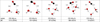 |
Fig. 1 Model systems of CO–W2–3 used for the DFT energy and geometry benchmark. Rows show structure names and binding energies (BE). Numbers in parentheses indicate the ZPVE-corrected BE value. The water molecule acting as the H-bond donor to CO is labeled WD. Characteristic distances are given in Å; energy values are in K. Atoms are color coded as follows: black for C, red for O, and white for H. |
 |
Fig. 2 Upper panel: top view of one of the nonporous (npASW) (left) and porous (pASW) ice models. Each periodic surface contains 500 water molecules. Lower panel: altitude plot relative to the same two structures (see Appendix D). Periodic cell dimensions are indicated. Distances are given in Å. |
2.5 Binding site sampling and optimization and binding energy distributions
After preparing npASW and pASW models, we sampled both surfaces with the CO molecule. The sampling algorithm consists of five steps.
A grid of equispaced points is generated as initial guesses for the CO positions on the ice surface. Each new point is located 3 Å from its nearest neighbor. We introduced noise on the grid points by relaxing the grid coordinate by ±1/4 of the step size in both X and Y directions.
The CO molecule is placed at a grid point and positioned so that its center of mass is at a specific distance from the nearest neighboring surface atom. We performed three rounds of sampling with initial distances of 2.50, 2.75, and 3.00 Å from the surface grid point. The initial CO orientation is randomized through a series of random Euler rotations.
Each initial structure is fully optimized using the MLP. The final number of binding sites varies among systems because the cell volume depends on the cell density.
The minima obtained from the initial surface model (resulting from the three sampling rounds) are filtered, grouping the structures based on a similarity threshold of root-mean-square deviation (RMSD) of atomic positions ≤0.07 Å.
The underlying points of the resulting BE distribution (BEd) were classified into five groups based on their deviation from the average BE, avg(BEd), using quartile (25%) intervals:
Very Low (VL): BE < avg(BEd) × 0.5
Low: avg(BEd) × 0.5 < BE < avg(BEd) × 0.75
Medium: avg(BEd) × 0.75 < BE < avg(BEd) × 1.25
High: avg(BEd) × 1.25 < BE < avg(BEd) × 1.5
Very High (VH): BE > avg(BEd) × 1.5.
Finally, we used a bootstrap method to obtain the mean (µ) and standard deviation (σ) of the BEd, taking into account the uncertainties derived from the MLP BE computations (Appendix E shows the details of this protocol).
3 Results
3.1 Fundamental nature of the CO-ASW interaction
3.1.1 Binding modes and binding energies in CO–W2–3 model systems
Carbon monoxide has a weak dipole moment of 0.112 Debye (Muenter 1975), with a small partial negative charge on the carbon end. This slightly predisposes CO to bind to a polar water ice surface in a low-temperature environment. To elucidate this interaction and identify different binding modes, we probed the CO interaction with small water clusters (the water dimer and trimer, W2–3). The different binding modes are shown in Fig. 1, together with the ZPVE- corrected BEs. The BEs of all the identified binding modes lie between 300 and 1500 K, with CO establishing weak hydrogen bonds (H-bonds) to the water molecules both through the carbon and oxygen ends. However, the binding mode with the highest BE corresponds to the dimer structure in which an interaction is established through the carbon end of CO that harbors the partial negative charge (CO – W2 – a). Interestingly, the equivalent binding mode in the trimer structure (CO – W3 – a) shows a decrease in BE of 638 K. The addition of a third water molecule results in higher rigidity by creating a H-bond cycle; consequently, the CO molecule’s interaction with the pair of water molecules becomes less energetically favorable. To gain further insights into the drivers of CO binding, we decompose the contributions to the BE in the Appendix (Table A.6). The structure with the lowest BE (CO – W3 – c) uniquely exhibits a notable deformation energy, as it disrupts the H-bond cycle of the water trimer. However, this structure still has a positive BE, due to a very favorable interaction energy (the highest among the five binding sites), as it takes part in a cyclic structure. This is noteworthy because such H-bond network imperfections can occur naturally in ASW owing to adjacent water molecules, thereby creating a high-BE environment for CO.
Interaction energies (IE) obtained at the different symmetry-adapted perturbation (SAPT) flavors.
3.1.2 SAPT analysis of the CO binding
Table 1 reports the dispersion factor (Fdisp, Eq. (6)) calculated for the model systems using SAPT at various levels of accuracy, as an indication of the dispersion character of the binding. The individual contributions are reported in Appendix Table A.7. The dispersion factor is small for the model systems structures, ranging from 0.21 to 0.53, indicating that CO binds to the small water clusters predominantly through electrostatic and induction interactions. Only in CO – W3 – b does the dispersion interaction represent more than 50% of the attractive contributions of the interaction energy. The electrostatic and induction attractive contributions are larger when CO interacts with a dangling OH bond (water H atoms that are not engaged in any H bond with other water molecules) via the C-extremity, as in the water dimer CO – W2 – a and trimer CO – W3 – a, CO – W3 – c. These structures also exhibit the highest net interaction energy. However, the electrostatic contribution in CO – W2 – a and CO – W3 – c is more than twice that of CO − W3 − a. Such enhanced interaction in these structures – in which CO interacts only with a water dimer – is attributable to the fact that the H bond established to CO is the sole donor interaction for that water molecule (namely WD in Fig. 1). In contrast, in CO − W3 − a, where a H-bond cycle is established in the water trimer, WD also acts as a H-bond donor to a second water molecule. This exclusive donor interaction, established in CO − W2 − a and CO − W3 − c, is reflected in the closer proximity of the CO molecule to WD, and renders WD more electron-deficient, intensifying the electrostatic coupling with the negatively charged carbon end. Analysis of the dispersion interaction reveals that this contribution is significantly lower than the electrostatic and induction contributions. Nevertheless, for CO − W3 − b, the balance between dispersion and electrostatic and induction interactions is slightly shifted toward dispersion, resulting in a dispersion factor of 0.53. This is consistent with the binding mode in CO − W3 − b, in which CO is positioned within the triangle formed by the H-bond network of the water molecules in the trimer cluster. However, due to the closer proximity of the CO molecule to the closest water trimer in CO − W3 − b, the exchange repulsion is significant and higher than in CO − W3 − a (See Table 1). Finally, a comparison of the Fdisp values obtained using SAPT/jun-cc-pVDZ and SAPT0-D3MBJ/aug-cc-pVDZ against the more accurate SAPT2+/aug-cc-PVDZ reveals that SAPT0-D3MBJ yields a Fdisp that aligns significantly better with the reference value than SAPT0.
3.2 ASW surface characterization
We modeled two sets of ASW surfaces following the procedure described in Sect. 2.4. The first set, labeled nonporous (np) ASW, consists of smooth surfaces, while the second set, porous (p) ASW, features uneven surfaces with protrusions and cavities. To characterize and visualize the ice models, we reconstructed the interface using a triangular 3D surface (tri-surface) interpolation method (see Appendix D). This allowed us to identify the surface atoms and quantify properties such as the areal average roughness (Sa, Eq. (D.1)), and the mean roughness depth (Rz, Eq. (D.2)). The Sa, estimated as the sum of the deviations from the mean plane of the surfaces, is 3.0 Å for the np ASW model and increases for the pASW model, reaching 3.8 Å. The Rz, averaging the five largest distances in altitude, yields 15.8 Å for np ASW and 18.4 Å for pASW. These values confirm that the pASW model has a larger surface area and deep hollow regions resembling nanopores. The nanopores are roughly spherical open cavities with widths ranging from 2 to 15 Å, and the ratio between the height of the cap (L) and the radius of the sphere cavity (Rs), L/Rs, is less than 1. The degree of roughness is important because high roughness (i.e., for almost closed cavities L/Rs ~ 2) is suggested to increase the probability that molecules desorbing from the grains collide with the pore walls, resulting in re-adsorption (Maggiolo et al. 2019). The magnitude of Rz for pASW models allows the identification of distinct valley and peak regions, representing portions of the surface that differ most in altitude and offer the most diverse binding sites for adsorbates. Another factor affecting CO adsorption is the presence of dangling OH bonds. These bonds typically point upward with from the surface and are pivotal in determining binding site characteristics (Al-Halabi et al. 2004; Nagasawa et al. 2021; Bovolenta et al. 2024). The estimated percentage of dangling OH bonds (%d(OH)) reveals a notable difference between the models: 6.9 and 10.8 for npASW and pASW, respectively. The lower value in the npASW model is due to its more compact structure, where more H bond interactions are established within the ice, reducing the number of dangling OH bonds.
Fig. D.1 shows the location of the dangling OH bonds in the different models. Notably, dangling OH bonds are also present on the inner surfaces of the nanopores.
3.3 Statistical nature of CO interaction with water
3.3.1 Binding energy distributions
Fig. 3 shows the BEd for the two different surfaces of ASW, representing the core results of this study. The CO-npASW and CO-pASW BE distributions comprise 415 and 674 unique binding sites, respectively. A statistical analysis of the quartiles of the distributions defines the five BE intervals: Very Low (VL), Low, Medium, High, Very High (VH) (see Sect. 2.5 and Table 2 for details). Both BEd have a similar mean BE of approximately 1100 K, which decreases to 889 K for the npASW surface and 911 K for pASW after adding the ZPVE correction. Thus, it is important to highlight that the existence of the nanopores does not significantly affect the statistical BE profile of CO on ASW. One notable difference is the longer high-BE tail in the pASW, reflected in a higher maximum BE value of 1845 K compared with 1662 K for npASW. The significant standard deviations (σ: 277 and 292 K for npASW and pASW, respectively) relative to the mean BE values reflect the wide range of binding sites on these realistic, amorphous surfaces. This structural diversity enables the CO molecule to explore an extensive variety of adsorption configurations, effectively sampling the full spectrum of binding modes possible, resulting in broad BE distributions. The similarity of both BE distributions is somewhat surprising, given that npASW and pASW surfaces differ in nanopore features and the number of dangling OH bonds. In the next section, we rationalize these results using SAPT analysis of the binding sites.
3.3.2 Distribution of interaction energy components
To explain the similarities in the BEd of CO adsorbed on npASW and pASW, we estimated the interaction energy contributions for all binding sites. Due to system size limitations, we performed a SAPT analysis considering the 28 water molecules closest to CO’s center of mass in each binding site. The size of the extracted clusters was chosen according to our tests, which showed that the different contributions of the interaction energy converge after 22–25 molecules (see Fig. F.2 for convergence examples). We aimed to statistically evaluate the characteristics of CO interactions with the two types of ASW surfaces. From the interaction energy contributions, we also evaluated Fdisp ( Eq. (6)), whose distribution is reported in Fig. 4 (left panels) for the two ASW models, mapped on top of the bins of the ZPVE-corrected BE distributions. For both BE distributions, CO is bound by an interplay of electrostatic and dispersion interactions in the majority of binding sites. Structures of this type (ED-class, gray bins) are present across all BE regimes. One noticeable difference between both surface types is that in npASW there is a higher percentage of structures that are bound primarily by dispersion (Disp-class, orange bins, 33%) and fewer by electrostatic interactions (Elst-class, blue bins, 7%), whereas in p-ASW both groups are present in similar proportions (23 vs. 21% for Elst- and Disp-class, respectively). This difference can be attributed to the surface morphology (Sect. 3.2): the npASW surfaces contain fewer dangling OH bonds and more small surface gaps, where the CO can bind effectively through dispersion interactions. Conversely, the pASW exhibits more crests and valleys, which results in a larger proportion of dangling OH that facilitates electrostatic coupling.
The Elst-class displays the highest average BE for pASW (941 K), whereas in npASW both ED-class and Elst-class have practically the same value of 930 K. In both surfaces, the structures bound by dispersion (Disp-class) are mostly located in the center and low BE part of the distribution, while the high-BE tail (VH-BE group, violet bar in Fig. 3) is predominantly populated by ED-class structures. To better understand the characteristics of the VH-BE ED-class structures, we analyzed two representative examples predominantly bound by electrostatics or dispersion. These examples are shown in the insets of Fig. 5. Since they derive from the same ice model, the figure also shows their location (each binding site is optimized individually, and the figure shows the overlap of their ice altitude maps). The VH-BE Elst-class (BE = 1370 K, blue inset) is characterized by the presence of a water molecule acting as a H-bond to the C-extremity of the adsorbate. Within this binding site, the two water molecules closest to the CO molecule do not engage in hydrogen bonding with each other, reflecting a configuration akin to that observed in CO − W3 − c. This binding site shares structural parameters with CO − W3 − c, including bond distances and Fdisp value. Interestingly, this binding motif on the ASW surface is enabled by irregularities in the ASW framework, so the adsorption process does not require the large deformation energy observed in CO − W3 − c, resulting in a highly favorable binding site, with a non-ZPVE-corrected BE similar to the CO − W3 − c interaction energy. In fact, as shown in the example provided in Fig. 5, only three water molecules are located within a radius of 4.5 Å from the center of mass of CO, resembling a water trimer.
To extend this observation to other structures in Elst-class, we quantified the number of nearest neighboring water molecules for each binding site. This was determined by counting water molecules within a radius of 4.5 Å from the center of mass of CO (Nneigh). The results of this analysis are presented in the right panels of Fig. 4. For Elst-class interactions on both surfaces, significantly fewer water molecules surround the binding sites compared to other interaction types, reaching a maximum of Nneigh of four for np-ASW and six for p-ASW. This is expected because, for electrostatic interactions to be dominant, a specific arrangement of water molecules needs to be present, which limits crowding at the binding site.
In contrast, the binding environment for Disp-class molecules is quite different. An example is shown in the orange inset of Fig. 5. In this structure, the CO molecule is “floating” on the bottom of a concave ice portion, without establishing strong interactions with individual water molecules, and thus dispersion interactions with the ASW surface dominates. Naturally, this arrangement is not represented in the small water clusters (Fig. 1) and provides an exceptionally high dispersion energy (Edisp) value (2600 K; see Table A.1 for comparison), benefiting from the proximity of several water molecules (Nneigh = 9). A broader inspection of this interaction type, compared with the Elst-class, is shown in the right panels of Fig. 4. While Disp-class binding sites generally exhibit lower BEs at low coordination (i.e., when few water molecules are present within a 4.5 Å radius), their BE increases significantly as surrounding water molecules accumulate. This provides direct evidence of the long held intuition that stronger binding occurs in confined cavities. Nevertheless, the incremental SAPT analysis (Appendix F, Figure F.2) shows that the contribution of Edisp approaches convergence upon inclusion of 9–11 water molecules, thus additional water molecules situated at greater distances contribute only marginally to the overall dispersion energy. The ED-class structures exhibit characteristics of both Elst- and Disp-classes, such as the favorable interaction given by the establishment of H bonds with the ice and additive dispersion contributions increasing with surrounding water molecules. A typical VH-BE ED structure is highly embedded in the ASW network- as the adsorbate forms H bonds with the substrate- and is located in a valley region, benefiting from the closeness of several water molecules. A representative example is shown in Fig. F.1.
In summary, despite the average BE values and the shape of the BEd being comparable for CO-npASW and CO-pASW, a closer inspection of the interactions between CO and the surfaces reveals noticeable differences arising from their distinct morphological characteristics. Specifically, the higher abundance of dangling OH bonds on p-ASW promotes a comparatively stronger electrostatic binding regime (Elst-class) through hydrogen bonding with the substrate. Furthermore, the high-BE tail of the BEd in both ASW types is predominantly composed of ED-class structures, which benefit significantly from the presence of dangling OH bonds in conjunction with additive dispersion interactions due to the close proximity of multiple water molecules to CO. The in-depth analysis presented in this section provides a basis for future studies of adsorbates on pASW. Although we find similar BE distributions, CO likely represents a special case among the broad spectrum of possible adsorbates, due to the delicate interplay between electrostatic and dispersion inter-actions. We anticipate that more polar adsorbates will exhibit stronger binding to pASW, due to the higher density of dangling OH bonds in this model. If confirmed, this behavior may have significant implications for the segregation of polar and apolar molecules on ice surfaces. We intend to explore this line of research further in future studies.
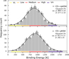 |
Fig. 3 Histograms of the ZPVE corrected BEs obtained for CO adsorbed on five npASW (upper panel) and five pASW surfaces (lower panel). The color-coded bars below each panel indicate the BE groups (VL: Very Low, Low, Medium, High, and VH: Very High). Gaussian fits were obtained using the bootstrap procedure detailed in Appendix E, which propagates individual uncertainties from the neural-network models into the Gaussian fitting procedure. |
 |
Fig. 4 CO-npASW panel showing (left) BE distribution for CO on npASW ice, with color mapping highlighting the dominant interaction contributions at various binding sites, ranging from primarily electrostatic (Elst-class, blue) to purely dispersion (Disp-class, orange), while ED-class (gray) represents an intermediate group. The coefficient that determines the class of a binding site is the ratio between the dispersion energy and the sum of the attractive interaction energies (electrostatic, induction, and dispersion), as defined in Sect. 2.2. (Right) Correlation between the BE and CO number of neighbors (i.e., the number of water molecules within a radius of 4.5 Å of the CO center of mass) for each class of binding sites. Averages are shown as points connected by a dashed line, and the standard deviation is shown as a shaded region of matching color. CO-pASW panel: Analogous data for pASW ice. |
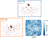 |
Fig. 5 Example of Very High (VH)-BE structures belonging to the Elst-class (blue, BE = 1370 K) and Disp-class (orange, BE = 1492 K), and their location on the pASW surface, represented as an altitude map. The inset figures display a portion of the binding sites comprising 50 water molecules, represented as sticks. Water molecules within 4.5 Å of the CO center of mass (i.e., nearest neighbors, Nneighb) are highlighted. |
3.4 Simulated TPD curves
Our detailed BE map allows the generation of realistic TPD curves akin to those observed in multicoverage TPD experiments. To this end, it is essential to consider that CO molecules can diffuse as the temperature increases prior to the onset of desorption. The extent of the diffusion depends on the initial CO coverage of the substrate: at full coverage, diffusion is restricted because all binding sites are occupied. As the initial coverage decreases, molecules gain the ability to diffuse into empty binding sites, particularly those with higher BE. Consequently, desorption predominantly occurs from these higher-BE sites. With a complete BE distribution, it is possible to simulate various scenarios corresponding to different degrees of coverage. Specifically, by applying progressively left-truncated distributions (excluding low BE sites) it is possible to approximate desorption behavior under different conditions and to analyze scenarios in which only high-BE sites remain available. In total, we computed TPD traces considering four different truncations of the BEd, and two pre-exponential factors, following the procedure explained in Appendix G. We used a heating rate of 0.3 Ks−1 which lies within the range commonly used in multicoverage TPD experiments (0.2–0.5 K s−1). The initial coverage (θi) corresponds to the fraction of remaining binding sites after truncation of the BEd. Fig. 6 shows the results for CO-npASW (upper panel) and CO-pASW (lower panel). The solid and segmented lines correspond to TPD traces derived with a pre-exponential factor of v = 1012 s−1 and v = 9.14 × 10¹⁴ s−1, respectively. Simulated scenarios with lower coverages (i.e., corresponding to left-truncated distributions with higher BEs) yield TPD traces shifted to higher temperatures and with lower desorption flux, consistent with experimental TPD traces. The TPD peaks for high-coverage cases lie around 30 K, while for low-coverage cases they are located around 50 K. The higher pre-exponential factor (segmented line) shifts the TPD traces by 8–9 K to lower temperatures, consistent with faster desorption kinetics associated with an increased desorption attempt frequency. The TPD traces from all the truncations exhibit a common tail toward higher temperatures, as expected, since they all stem from the same high-BE bins desorption flux. Notably, this feature is also observed in multicoverage TPD experiments. Finally, the results for CO-npASW and CO-pASW closely resemble each other, reflecting the similarity of their BEd.
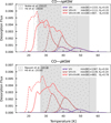 |
Fig. 6 Simulated TPD traces using BE distributions from our study compared to different experimental results of multicoverage TPD desorption from Noble et al. (2012b), Nguyen et al. (2018), and He et al. (2016). The heating ramp rate (β) is 0.3 K s−1 (See Appendix G for further details). Different colored TPD traces correspond to simulations considering different BE cutoffs in the distribution, excluding BEs lower than min(BE)(see Table 3). The initial coverage for each TPD trace corresponds to the fraction of molecules of the full distribution remaining after applying the cutoff. The shaded area represents the range of experimental TPD results. Two pre-exponential factors are shown: v = 1012 s−1 (solid lines) and v = 9.14 × 10¹⁴ s−1 (dashed lines), the latter is derived from transition state theory as detailed in Minissale et al. (2022). |
4 Discussion
4.1 Comparison with experimental TPD results
To assess the relation between our BE distributions and the experimental BEs derived from TPD experiments, we directly compared our simulated TPD traces with three experimental results (Noble et al. 2012b; Nguyen et al. 2018; He et al. 2016), that reported multicoverage TPD traces for CO bound to different ASW types. The temperature regions corresponding to the desorption fluxes observed from these experiments are depicted as shaded areas in Fig. 6. The simulated traces fall largely within the experimental ranges across all studies. In both the experimental and theoretical TPDs, the signals corresponding to pASW are shifted to higher temperatures compared to npASW, consistent with the longer high-BE tails observed in the CO-pASW distribution. However, for the high-coverage cases, the simulated TPD traces are slightly shifted to lower temperatures relative to the experimental results. This discrepancy may arise from lateral CO-CO interactions, which are not present in our simulated TPD traces and could affect the desorption profile in that regime.
The pre-exponential factor has a noticeable effect on the position of the signals in the simulated TPD spectra. The pre-exponential factor derived from transition state theory (TST) (v = 9.4 × 10¹⁴ s−1 (Minissale et al. 2022)) shifts the TPD traces (segmented lines in Fig. 6) to lower temperatures, resulting in poorer agreement with the experimental results. When comparing simulated TPD curves to experimental ones, it is important to mention that Bariosco et al. (2024) recently generated simulated TPD traces derived from ab initio H2S BEd on a large cluster ASW model. In their work, they detected a shift to lower temperatures for the simulated TPD relative to the experimental results. However, the shift is much larger than that observed here, which is puzzling since the diffusion of H2S should be lower than in the case of CO, as the molecule can interact through hydrogen bonding to the surface and has a much higher interaction energy with the ASW surface. The disagreement with experimental results in the case of H2S simulated TPD traces most likely stems from an overestimation of the ZPVE correction of the BE values, which was computed for every binding site using embedding procedures and may have contributed to the discrepancy.
BEs and TPD peaks for different binding energy regimes.
4.2 Comparison with theoretical binding energy values
Over the years, many attempts have been made to compute the CO – water interaction using force fields or quantum chemistry methods. Karssemeijer et al. (2013) studied the interaction of one to six CO molecules on ASW using classical force fields parametrized with high-level ab initio data of the H2O-H2O and H2O-CO dimers. Similar to the present work, they obtained a BEd, albeit shifted to higher energies (650–2900 K). The difference may be ascribed to the inability of force fields to fully capture the many-body polarization and subtle orientation-dependent interactions in complex, disordered environments like ASW. Because the interactions in force fields are parametrized on ideal model systems, the resulting BE values are naturally higher than those reported here, which were obtained using an MLP trained on a wide range of realistic ASW-like cluster configurations. The only other BEd for CO-ASW was presented by Bovolenta et al. (2022), who employed a set of amorphized water clusters containing 22 molecules each as a surface model. Using the ω-PBE/def-TZVP//M05/def-TZVP level of theory together with BSSE correction yielded a non-ZPVE corrected average BE of 1035 K, which is slightly lower than the one reported in this study. However, the standard deviation of the set-of-clusters model BE distribution was significantly lower, with a value of 176 K versus 277-292 K reported in this work. Because such medium-sized clusters have a higher proportion of dangling OH bonds compared to both npASW and pASW models, the narrower distribution can be rationalized by examining the Elst-class binding sites defined in this study, which are likely predominant in the cluster model. Within this class, the spread of BEs is considerably lower (See Fig. 4, blue bins), while the average BE remains similar to the total average BEd and across all three classes. Therefore, the inclusion of dispersion-dominated structures appears to affect the spread of the BEd, while influencing the average to a lesser extent. Hence, a geometrical similarity between the set-of-clusters binding sites and the Elst-class sites would explain the analogous similarity in the average BE. A different approach was used by Ferrero et al. (2020), who obtained a range of BEs by placing CO on different sites of an amorphous water slab consisting of 60 water molecules. They used periodic systems at the B3LYP-D3/A-TZV level of theory to compute the BEs on HF-3c-optimized binding sites. The non-ZPVE-corrected BE range of 1300-2200 K falls within the high-BE half of the BEds presented in this study. This tendency is in agreement with our benchmark, which showed that the B3LYP-D3BJ method tends to overbind the small reference systems (see Appendix A), potentially contributing to the higher BEs. Additionally, the HF-3c level of theory for binding-site optimization may not be sufficiently reliable for accurately describing CO-H2O interactions (Bovolenta et al. 2022). Concurrently with this study, Groyne et al. (2025) obtained a BEd on ASW using a multi-level approach. They first built an ASW model with a classical force field, from which they extracted and sampled a hemisphere using ONIOM2 embedding. In their scheme, the high-level zone (the binding site and molecules within 8 Å) was treated at the B3LYP-D3BJ/6-311G(d,p) level of theory, while the low-level region was treated with the GFN2-xTB method. Their ZPVE and BSSE corrected BE is higher than the one presented here, amounting to an average value of 1400 K and a standard deviation of 340 K. The significantly higher values in their work are puzzling, as the ASW surface they prepared is similar to that presented here. A source of discrepancy could be the level of theory, since B3LYP-D3BJ tends to overestimate the BE of CO + ASW. Another possible source of discrepancy is the polarization from the outer, GFN2-treated, region in the ONIOM2 calculation. This term contributed up to 25% of the total BE, a surprisingly large influence given the considerable size of the high-level zone. In contrast, the SAPT0-D3BJ incremental analysis presented here demonstrates that more distant molecules have a negligible effect on the interaction energy. Further studies comparing the two approaches will be needed to reconcile these differing results.
4.3 CO snowlines in protoplanetary disk from our derived distributions
One of the key quantities used to characterize the distribution of molecules in protoplanetary disks (PPDs) is the so-called snowline, typically defined for H2O. This snowline marks the region in the disk where water vapor condenses into ice, setting the boundary between the formation zones of rocky and gas giant planets (Notsu 2020). In this context, predicting the corresponding snowline for CO is crucial for understanding the distribution of organic molecules within PPDs, as well as the organic inventory available to forming planets.
To contextualize our results under this prism, we simulated the CO partitioning between the gas and solid phases at each position in a 2D protoplanetary disk model. We used the density and temperature profiles for gas and dust, together with the stellar UV radiation field appropriate for the TW Hya disk (Cleeves et al. 2015; Furuya et al. 2022b). We assumed a total (gas + solid) CO abundance relative to H nuclei of 10^4 throughout the disk. In the disk atmosphere, however, the strong UV radiation from the central star dissociates CO. Accordingly, no CO molecules were assumed to exist in regions with AV < 1 mag (Aikawa & Nomura 2006).
The partitioning of CO between the gas phase and the solid phase was calculated in two ways. In a first approach, we used our BEd of CO on npASW to calculate the partitioning in a manner similar to that of Tinacci et al. (2023); at each disk position, we calculated the fraction of adsorption sites where kthdes > kads (ƒgas), and the gas-phase and solid-phase CO abundance at each disk position were given by 10−4ƒgas and 10−4(1 − ƒgas), respectively. Here kthdes and kads are the rate constants for thermal desorption and adsorption of CO, respectively. In a second approach, we compared kthdes evaluated with the mean binding energy of CO on p-ASW with kads at each disk position. When the former exceeded the latter, all CO molecules were assumed to exist as vapor; when it was smaller, all CO molecules were assumed to exist as ice. In both cases, the pre-exponential factor v for kthdes was set to 1012 s−1. Tests with v=9.14× 10¹⁴ s−1 did not yield significant changes.
Fig. 7 shows the 2D (radial + vertical) distribution of gas-phase and solid-phase CO using the multibinding description (right) and the single-binding description (left). In the single-binding description, the partitioning of CO between the gas and solid phases dramatically changes around 20–25 K, above which CO is predominantly present in the gas phase, while below it CO resides mainly in the solid phase. The CO snowline (or snow surface) can therefore be defined as a temperature of 20–25 K. Conversely, in the multibinding description, a non-negligible fraction of CO exists in the gas phase even at 15 K, while a comparable fraction of CO remains in the solid phase even at 30 K. Therefore, the CO gas and ice coexist in larger regions of the disk in the multibinding description than in the single-binding description. This effect is evident in the vertically integrated CO gas and ice column densities shown in Fig. 8.
The change in snowlines indicated by our results carries important implications for the chemistry of PPDs. Because CO is considered the most important precursor of complex organic molecules through reactions on ice (Watanabe & Kouchi 2002), changes in this feedstock affect the overall distribution of organics in PPDs. The multibinding approach suggests a broader spatial extension of CO in the disk midplane and beyond, along with a corresponding enhancement in its gas-phase distribution, driven by the presence of both high- and low-binding-energy sites. This contrasts with the predictions of a single-binding approach, which imply a richer CO chemistry at low stellar radii. Finally, our results reproduce the trend predicted by Grassi et al. (2020) for CO partitioning using BE distributions, providing a quantitative estimate of their effect.
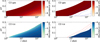 |
Fig. 7 Two dimensional spatial distributions of CO gas (upper panels) and ice (lower panels) abundances on the disk, shown using a multibinding description (left panels) and a single binding description (right panels). The vertical axes represent height normalized by radius. Dashed lines depict the positions where the dust temperature is equal to 30, 25, 15, and 10 K. |
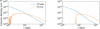 |
Fig. 8 Vertically integrated CO gas and ice column densities as functions of radius. The left panel shows the model with the multibinding description, while the right panel shows the single binding description. |
4.4 Implications for other astrophysical regions
Adopting a multibinding approach to the BE has direct implications for PPDs, as discussed above. In the context of cold molecular clouds, however, the implications are different. At ultracold temperatures (~10 K), adopting a multibinding approach has a negligible effect on the desorption rates (Fig. 6); however, it can significantly influence CO diffusion, and, consequently, the formation of CO-related species. This has already been demonstrated in our previous studies (Molpeceres et al. 2024; Furuya 2024), particularly for reactions involving CO other than hydro-genations, most notably in the case of CO2 formation. In warmer regions such as hot cores, the multibinding approach is expected to have little impact, since CO is not significantly depleted onto dust grains under these conditions.
5 Conclusions
This paper presents the binding energy distributions of CO bound to porous and nonporous amorphous solid water surfaces. We used a machine-learning potential trained on forces and energies of CO interacting with differently sized clusters (W22 − W60), computed at the MPWB1K-D3BJ-gCP/def-TZVP level. The main results of this study can be summarized as follows.
Quantifying the interaction of CO on small water clusters at a high level of theory (CCSD(T)/CBS) allowed us to construct a DFT benchmark to select a suitable model chemistry for training the MLP. In small clusters, BEs span approximately 300 and 1500 K, generally decreasing when additional water molecules form more rigid hydrogen-bonded networks. Symmetry-adapted perturbation theory (SAPT) analyses highlight the dominance of electrostatic and induction interactions, while dispersion contributes less significantly in these small systems.
An analysis of the compact nonporous (npASW) and porous (pASW) surfaces reveals significant morphological differences between them. The porous surfaces exhibit greater roughness, deeper valleys, and higher densities of dangling OH bonds compared to the smoother nonporous surfaces. Quantitative metrics, such as areal average roughness and mean roughness depth, confirm these structural differences.
The binding energy distributions obtained for these systems exhibit Gaussian-like shapes with mean zero-point vibrational energy-corrected values near 900 K, showing little overall difference between porous and non-porous surfaces. Interaction energy decomposition, however, reveals important differences: pASW favors electrostatic interactions due to the higher density of dangling OH groups, while npASW exhibits a greater proportion of dispersion-dominated binding sites. High-BE sites typically involve balanced contributions from both electrostatic and dispersion interactions, highlighting the intricate interplay between local morphology and molecular-level interactions. These findings emphasize the complexity and diversity of CO adsorption on ASW, which is relevant for accurately modeling astrochemical processes. The limited variability in the binding energy distributions of CO on npASW and pASW, resulting from a balance between electrostatic and dispersion interactions, suggests that the observed independence from substrate morphology is a unique characteristic of CO and perhaps other apolar molecules such as CO2 or CH4. This behavior is unlikely to extend to polar adsorbates, such as NH3 or CH3OH, which are expected to exhibit binding energy distributions shifted toward stronger binding on pASW, due to the uneven distribution of dangling OH bonds.
We propose a new approach to compare full binding energy distributions to experimental TPD studies based on truncation of the distribution to mimic a low-coverage scenario and diffusion to high-binding energy sites before desorption. Using this approach, we effectively reproduce the main features observed experimentally in multicoverage TPD curves of CO on ASW surfaces. We find that our simulated TPD traces mostly fall within the experimental peaks range (25–55 K).
Compared to single-value models, our multibinding-energy approach results in a broader and more diffuse CO snowline in protoplanetary disks, significantly extending the region where CO ice and gas coexist. This expanded coexistence zone, spanning approximately 15–30 K, indicates more complex partitioning between gas and ice phases, which carries critical implications for chemical evolution and organics delivery in planet formation scenarios within protoplanetary disks.
We aim to expand this novel methodology for the computation of binding energies, taking into account realistic statistical characteristics inherent to ASW surfaces, to other important interstellar molecules.
Data availability
Molecular structures, energies, and forces used for training the machine learning potential can be accessed online2. Additional information is available from the corresponding authors upon request.
Acknowledgements
G.M.B. gratefully acknowledges support from Proyecto UCO 1866 Beneficios Movilidad 2021-2022. G.M. acknowledges the support of the grant RYC2022-035442-I funded by MICIU/AEI/10.13039/501100011033 and ESF+. G.M. also received support from project 20245AT016 (Proyectos Intramurales CSIC). We acknowledge the computational resources provided by bwHPC and the German Research Foundation (DFG) through grant no INST 40/575-1 FUGG (JUSTUS 2 cluster), the DRAGO computer cluster managed by SGAI-CSIC, and the Galician Super- computing Center (CESGA). The super-computer FinisTerrae III and its permanent data storage system have been funded by the Spanish Ministry of Science and Innovation, the Galician Government, and the European Regional Development Fund (ERDF). S.V.G. thanks VRID research grant 2022000507INV for financing this project. This work was funded by Deutsche Forschungsgemeinschaft (DFG, German Research Foundation) under Germany’s Excellence Strategy - EXC 2075 - 390740016. We acknowledge the support of the Stuttgart Center for Simulation Science (SimTech).
References
- Aikawa, Y., & Nomura, H. 2006, ApJ, 642, 1152 [Google Scholar]
- Al-Halabi, A., Fraser, H. J., Kroes, G. J., & Van Dishoeck, E. F. 2004, A&A, 422, 777 [NASA ADS] [CrossRef] [EDP Sciences] [Google Scholar]
- Amiaud, L., Fillion, J. H., Baouche, S., et al. 2006, J. Chem. Phys., 124, 094702 [Google Scholar]
- Bannwarth, C., Ehlert, S., & Grimme, S. 2019, J. Chem. Theor. Comput., 15, 1652 [Google Scholar]
- Bariosco, V., Pantaleone, S., Ceccarelli, C., et al. 2024, MNRAS, 531, 1371 [NASA ADS] [CrossRef] [Google Scholar]
- Bossa, J.-B., Isokoski, K., Paardekooper, D. M., et al. 2014, A&A, 561, A136 [NASA ADS] [CrossRef] [EDP Sciences] [Google Scholar]
- Bovolenta, G. M., & Vogt-Geisse, S. 2025, J. Mol. Model, 31, 104 [Google Scholar]
- Bovolenta, G., Bovino, S., Vöhringer-Martinez, E., et al. 2020, Mol. Astrophys., 21, 100095 [NASA ADS] [CrossRef] [Google Scholar]
- Bovolenta, G. M., Vogt-Geisse, S., Bovino, S., & Grassi, T. 2022, ApJS, 262, 17 [NASA ADS] [CrossRef] [Google Scholar]
- Bovolenta, G. M., Silva-Vera, G., Bovino, S., et al. 2024, Phys. Chem. Chem. Phys., 26, 18692 [Google Scholar]
- Boys, S. F., & Bernardi, F. 1970, Mol. Ph., 19, 553 [Google Scholar]
- Bozkaya, U., & Sherrill, C. D. 2017, J. Chem. Phys., 147, 044104 [Google Scholar]
- Chaabouni, H., Diana, S., Nguyen, T., & Dulieu, F. 2018, A&A, 612, A47 [NASA ADS] [CrossRef] [EDP Sciences] [Google Scholar]
- Cleeves, L. I., Bergin, E. A., Qi, C., Adams, F. C., & Öberg, K. I. 2015, ApJ, 799, 204 [CrossRef] [Google Scholar]
- Clements, A. R., Berk, B., Cooke, I. R., & Garrod, R. T. 2018, PCCP, 20, 5553 [Google Scholar]
- Collings, M. P., Anderson, M. A., Chen, R., et al. 2004, MNRAS, 354, 1133 [NASA ADS] [CrossRef] [Google Scholar]
- Cuppen, H. M., & Herbst, E. 2007, ApJ, 668, 294 [Google Scholar]
- Cuppen, H. M., Walsh, C., Lamberts, T., et al. 2017, Space Sci. Rev., 212, 1 [Google Scholar]
- Das, A., Sil, M., Gorai, P., Chakrabarti, S. K., & Loison, J.-C. 2018, ApJS, 237, 9 [NASA ADS] [CrossRef] [Google Scholar]
- Dohnálek, Z., Kimmel, G. A., Ayotte, P., Smith, R. S., & Kay, B. D. 2003, J. Chem. Phys., 118, 364 [CrossRef] [Google Scholar]
- Duflot, D., Toubin, C., & Monnerville, M. 2021, Front. Astron. Space Sci., 8 [Google Scholar]
- Dunning T. H., J., Peterson, K. A., & Wilson, A. K. 2001, J. Chem. Phys., 114, 9244 [NASA ADS] [CrossRef] [Google Scholar]
- Fedoseev, G., Cuppen, H. M., Ioppolo, S., Lamberts, T., & Linnartz, H. 2015, MNRAS, 448, 1288 [NASA ADS] [CrossRef] [Google Scholar]
- Fedoseev, G., Scirè, C., Baratta, G. A., & Palumbo, M. E. 2017, MNRAS, 475, 1819 [Google Scholar]
- Ferrero, S., Zamirri, L., Ceccarelli, C., et al. 2020, ApJ, 904, 11 [NASA ADS] [CrossRef] [Google Scholar]
- Fuchs, G. W., Cuppen, H. M., Ioppolo, S., et al. 2009, A&A, 505, 629 [NASA ADS] [CrossRef] [EDP Sciences] [Google Scholar]
- Furuya, K. 2024, ApJ, 974, 115 [NASA ADS] [CrossRef] [Google Scholar]
- Furuya, K., Hama, T., Oba, Y., et al. 2022a, ApJ, 933, L16 [CrossRef] [Google Scholar]
- Furuya, K., Tsukagoshi, T., Qi, C., et al. 2022b, ApJ, 926, 148 [NASA ADS] [CrossRef] [Google Scholar]
- Grassi, T., Bovino, S., Caselli, P., et al. 2020, A&A, 643, A155 [EDP Sciences] [Google Scholar]
- Grimme, S., Antony, J., Ehrlich, S., & Krieg, H. 2010, J. Chem. Phys., 132, 154104 [Google Scholar]
- Grimme, S., Ehrlich, S., & Goerigk, L. 2011, J. Comput. Chem., 32, 1456 [Google Scholar]
- Groyne, M., Champagne, B., Baijot, C., & Becker, M. D. 2025, A&A, 698, A284 [NASA ADS] [CrossRef] [EDP Sciences] [Google Scholar]
- Gyorffy, W., & Werner, H.-J. 2018, J. Chem. Phys., 148, 114104 [CrossRef] [Google Scholar]
- Hama, T., & Watanabe, N. 2013, Chem. Rev., 113, 8783 [Google Scholar]
- He, J., Acharyya, K., & Vidali, G. 2016, ApJ, 825, 89 [Google Scholar]
- Helgaker, T., Klopper, W., Koch, H., & Noga, J. 1997, J. Chem. Phys., 106, 9639 [NASA ADS] [CrossRef] [Google Scholar]
- Herbst, E., & van Dishoeck, E. F. 2009, ARA&A, 47, 427 [NASA ADS] [CrossRef] [Google Scholar]
- Hjorth Larsen, A., Jørgen Mortensen, J., Blomqvist, J., et al. 2017, J. Phys. Condens. Matter, 29, 273002 [Google Scholar]
- Hunter, J. D. 2007, Comput. Sci. Eng., 9, 90 [NASA ADS] [CrossRef] [Google Scholar]
- Jeziorski, B., Moszynski, R., & Szalewicz, K. 1994, Chem. Rev., 94, 1887 [Google Scholar]
- Kalvans, J., Kalnina, A., & Veitners, K. 2024, A&A, 687, A296 [NASA ADS] [CrossRef] [EDP Sciences] [Google Scholar]
- Karssemeijer, L. J., Ioppolo, S., Hemert, M. C. v., et al. 2013, ApJ, 781, 16 [Google Scholar]
- Keane, J. V., Boogert, A. C. A., Tielens, A. G. G. M., Ehrenfreund, P., & Schutte, W. A. 2001, A&A, 375, L43 [NASA ADS] [CrossRef] [EDP Sciences] [Google Scholar]
- Kruse, H., & Grimme, S. 2012, J. Chem. Phys., 136, 154101 [Google Scholar]
- Maggiolo, R., Gibbons, A., Cessateur, G., et al. 2019, ApJ, 882, 131 [Google Scholar]
- Mariedahl, D., Perakis, F., Späh, A., et al. 2018, J. Phys. Chem. B, 122, 7616 [Google Scholar]
- McClure, M. K., Rocha, W. R. M., Pontoppidan, K. M., et al. 2023, Nat. Astron., 7, 431 [NASA ADS] [CrossRef] [Google Scholar]
- Minissale, M., Aikawa, Y., Bergin, E., et al. 2022, ACS Earth Space Chem., 6, 597 [NASA ADS] [CrossRef] [Google Scholar]
- Molpeceres, G., & Kästner, J. 2020, PCCP, 22, 7552 [NASA ADS] [CrossRef] [Google Scholar]
- Molpeceres, G., Zaverkin, V., & Kästner, J. 2020, MNRAS, 499, 1373 [Google Scholar]
- Molpeceres, G., Zaverkin, V., Furuya, K., Aikawa, Y., & Kästner, J. 2023, A&A, 673, A51 [NASA ADS] [CrossRef] [EDP Sciences] [Google Scholar]
- Molpeceres, G., Furuya, K., & Aikawa, Y. 2024, A&A, 688, A150 [NASA ADS] [CrossRef] [EDP Sciences] [Google Scholar]
- Muenter, J. S. 1975, J. Mol. Spectrosc., 55, 490 [NASA ADS] [CrossRef] [Google Scholar]
- Nagasawa, T., Sato, R., Hasegawa, T., et al. 2021, ApJ, 923, L3 [NASA ADS] [CrossRef] [Google Scholar]
- Neese, F., Wennmohs, F., Becker, U., & Riplinger, C. 2020, J. Chem. Phys., 152, 224108 [NASA ADS] [CrossRef] [Google Scholar]
- Nguyen, T., Baouche, S., Congiu, E., et al. 2018, A&A, 619, A111 [NASA ADS] [CrossRef] [EDP Sciences] [Google Scholar]
- Nguyen, T., Oba, Y., Shimonishi, T., Kouchi, A., & Watanabe, N. 2020, ApJ, 898, L52 [NASA ADS] [CrossRef] [Google Scholar]
- Noble, J., Dulieu, F., Congiu, E., & Fraser, H. 2012a, EAS Publ. Ser., 58, 353 [Google Scholar]
- Noble, J. A., Congiu, E., Dulieu, F., & Fraser, H. J. 2012b, MNRAS, 421, 768 [NASA ADS] [Google Scholar]
- Noble, J. A., Fraser, H. J., Smith, Z. L., et al. 2024, Nat. Astron., 8, 1169 [NASA ADS] [CrossRef] [Google Scholar]
- Notsu, S. 2020, Water Snowline in Protoplanetary Disks, Springer Theses (Singapore: Springer) [Google Scholar]
- Papajak, E., Zheng, J., Xu, X., Leverentz, H. R., & Truhlar, D. G. 2011, J. Chem. Theory Comput., 7, 3027 [Google Scholar]
- Parker, T. M., Burns, L. A., Parrish, R. M., Ryno, A. G., & Sherrill, C. D. 2014, J. Chem. Phys., 140, 094106 [Google Scholar]
- Perrero, J., Enrique-Romero, J., Ferrero, S., et al. 2022, ApJ, 938, 158 [NASA ADS] [CrossRef] [Google Scholar]
- Poštulka, J., Slavícek, P., Kästner, J., & Molpeceres, G. 2025, A&A, 697, A51 [NASA ADS] [CrossRef] [EDP Sciences] [Google Scholar]
- Raghavachari, K., Trucks, G. W., Pople, J. A., & Head-Gordon, M. 1989, Chem. Phys. Lett., 157, 479 [Google Scholar]
- Sameera, W. M. C., Senevirathne, B., Andersson, S., et al. 2021, J. Phys. Chem. A, 125, 387 [NASA ADS] [CrossRef] [Google Scholar]
- Schriber, J. B., Sirianni, D. A., Smith, D. G. A., et al. 2021, J. Chem. Phys., 154, 234107 [Google Scholar]
- Seung, H. S., Opper, M., & Sompolinsky, H. 1992, in Proceedings of the fifth annual workshop on Computational learning theory, Pittsburgh Pennsylvania USA, 287 [Google Scholar]
- Simons, M. a. J., Lamberts, T., & Cuppen, H. M. 2020, A&A, 634, A52 [NASA ADS] [CrossRef] [EDP Sciences] [Google Scholar]
- Smith, R. S., May, R. A., & Kay, B. D. 2016, J. Phys. Chem. B, 120, 1979 [Google Scholar]
- Sylvetsky, N., Kesharwani, M. K., & Martin, J. M. L. 2017, J. Chem. Phys., 147, 134106 [Google Scholar]
- Szalewicz, K. 2012, WIREs Comput. Mol. Sci., 2, 254 [Google Scholar]
- Tinacci, L., Germain, A., Pantaleone, S., et al. 2022, ACS Earth Space Chem., 6, 1514 [NASA ADS] [CrossRef] [Google Scholar]
- Tinacci, L., Germain, A., Pantaleone, S., et al. 2023, ApJ, 951, 32 [CrossRef] [Google Scholar]
- Wakelam, V., Loison, J. C., Mereau, R., & Ruaud, M. 2017, Mol. Astrophys., 6, 22 [NASA ADS] [CrossRef] [Google Scholar]
- Wang, L.-P. 2023,, https://github.com/leeping/geomeTRIC [Google Scholar]
- Watanabe, N., & Kouchi, A. 2002, ApJ, 571, L173 [Google Scholar]
- Weigend, F., & Ahlrichs, R. 2005, PCCP, 7, 3297 [Google Scholar]
- Werner, H.-J., Knowles, P. J., Knizia, G., Manby, F. R., & Schütz, M. 2012, WIREs Comput. Mol. Sci., 2, 242 [Google Scholar]
- Werner, H.-J., Knowles, P. J., Manby, F. R., et al. 2020, J. Chem. Phys., 152, 144107 [NASA ADS] [CrossRef] [Google Scholar]
- Zaverkin, V., & Kästner, J. 2020, J. Chem. Theor. Comput., 16, 5410 [Google Scholar]
- Zaverkin, V., Holzmüller, D., Schuldt, R., & Kästner, J. 2022, J. Chem. Phys., 156, 114103 [NASA ADS] [CrossRef] [Google Scholar]
- Zaverkin, V., Holzmüller, D., Steinwart, I., & Kästner, J. 2021, J. Chem. Theory Comput., 17, 6658 [Google Scholar]
- Zhao, Y., & Truhlar, D. G. 2005, J. Phys. Chem. A, 109, 5656 [NASA ADS] [CrossRef] [Google Scholar]
Appendix A Density functional theory benchmark
Focal point analysis of the binding energy for the CO − W2 − a structure.
Focal point analysis in kcal mol−1of the binding energy for the CO − W2 − b structure.
Appendix A.1 Reference energy
We used a total of five different binding sites to obtain a high-level binding energy from wavefunction methods. We optimized the binding site geometry at the CCSD(T)-F12/cc-pVDZ-F12 We computed the BEs on the different binding sites using the focal point analysis (FPA) technique to obtain a CCSD(T)/CBS quality value. In this approach, energy values computed at the SCF, MP2, CCSD, CCSD(T), levels of theory with the aug-cc-pVXZ basis sets. The total energy was extrapolated to the complete basis set limit (CBS) using the functional form:

where ESCF and ECORR are the extrapolated SCF and correlation energies (MP2, CCSD, CCSD(T)), respectively, and X is he cardinal number corresponding to the maximum angular momentum of the aug-cc-pVXC basis set (X=D,T,Q). A, B, C, E, and F are fitting parameters for the SCF and correlation energies, respectively. We used the extrapolation libraries implemented in the Psi4 driver together with the BEEP energy benchmark workflow. The binding energy was computed as usual: The binding energy (BE) of a species (i) adsorbed on a surface (ice) is defined as:
 (A.1)
(A.1)
where Esup is the energy of the super-molecule (CO+W) formed by the adsorbate bound to the water cluster, EW refers to the water cluster energy, and Ei is the energy of the adsorbate. Tables A.1–A.5 show the evolution of the contribution of electron correlation to the binding energy. In general the correlation converges smoothly when increasing the correlation level and basis set size, which gives binding energies of sub-chemical accuracy (uncertainty of approximately 0.1kcal mol−1 ≈ 50 K) so any DFT functional which yields BEs close to that accuracy is a good choice of model chemistry. Table A.6 shows the CCSD(T)/CBS values for the IE, DE, and BE of each of the model systems.
Focal point analysis in kcal mol−1of the binding energy for the CO − W3 − a structure.
Focal point analysis in kcal mol−1 of the binding energy for the CO − W3 − b structure.
Focal point analysis in kcal mol−1 of the binding energy for the CO − W3 − c structure.
Interaction energy, deformation energy, and binding energy at the CCSD(T)/CBS level of theory.
Table A.7 shows the different contributions to the IE, estimated at SAPT2+/aug-CC-PVDZ level. For the strongest binding mode in which the H-bond is established through the carbon end of the CO molecule. In both cases, the electrostatic energy represents the largest component of the interaction energy. Nonetheless, the electrostatic interaction energy in the dimer configuration is more than twofold that of the trimer. The enhanced interaction of CO within the water dimer is attributable to its engagement with a water molecule that solely acts as a H-bond acceptor, thereby rendering the water molecule more electron deficient and thus intensifying the electrostatic coupling with the negatively charged carbon end of the CO molecule. This is not the case in the trimer structure in which all water molecules are both receiving and donating H-bonds within a H-bond cycle. Furthermore this difference is accentuated in the polarization interaction, as the water dimer has a much greater ability to polarize the CO molecule than the water trimer. The dispersion interaction is significantly lower than the electrostatic interaction in both molecules, however for the trimer the dispersion represents a larger percentage of the total interaction energy with a dispersion factor of 0.3 compared to the water dimer structure which has a dispersion factor of 0.21. Finally due to the closer proximity of the CO molecule to the water dimer in its bound conformation, the exchange repulsion is quite significant and higher than in the water trimer. In summary, CO binds to the small water clusters predominately through electrostatic interactions. This contribution is larger when CO is directly interacting with a dangling water molecule as in the water dimer. However whenever a dangling-H bond is present, the interaction is weaker but the predominant mode of interaction is still electrostatic.
Interaction energy decomposition at the SAPT2+/aug-cc-PVDZ level of theory
Appendix A.2 DFT geometry and binding energy benchmark result
We probed 6 hybrid and meta-hybrid GGA functionals against the CCSD(T)-F12/cc-PVDZ reference geometry to evaluate which functional can best reproduce the binding site geometry of the CO − W2 − b and CO − W3 − b structures. The MPWB1K-D3BJ functional displays the lowest mean RMSD for describing the binding sites geometry of the model systems. Furthermore, we conducted a BE benchmark study on MPWB1K-D3BK/def2-TZVP geometries. The structures used for this benchmark were CO − W2 − a, CO − W2 − b and CO − W3 − b. The energies were compared to the BE values listed in Tables A.1, Table A.2 and Table A.4. The results of the best 15 of a total of 166 hybrid, meta-hybrid and long-range corrected DFT functionals MAE are shown in Table B.2. Again MPWB1K-D3BJ is one of the best performing DFT functionals with an average MAE of 63 K, which is within 40 K of the best performing functional. Given the good combined performance in gradients and BEs, the MPWB1K-D3BJ/def2-TZVP//MPWB1K-D3BJ/def2-TZVP model chemistry proves to be a suitable option for MLP training of gradients and energies. Nonetheless, it is important to note that this level of theory carries an uncertainty of at least 63 K in any BE prediction.
RMSD for the binding site geometry of the CO − W2 − b and CO − W3 − b structure with different hybrid and metahybrid DFT functionals.
Mean absolute error (MAE) in K of binding energies for benchmarked DFT functionals.
Appendix B ZPVE correction for the BEs
We determined ZPVE correction at the CCSD(T)-F12/cc-pVDZ-F12 level of theory through the calculation of the Hessian matrix and subsequent harmonic vibrational analysis on the four binding sites used in the DFT benchmark. Furthermore, we re-optimized the structures using DFT, specifically MPWB1K-D3BJ / def2-TZVP, and calculated the ZPVE correction at this level of theory as well. The ZPVE correction is reported as:
 (B.1)
(B.1)
where X = 2, 3. We also analyzed the impact of anharmonic correction to the vibrational frequencies using vibrational perturbation theory at the CCSD(T)/aug-cc-pVDZ level of theory using CFOUR software. We applied these corrections to two model systems, namely CO − W2 − a and CO − W3 − a. The results are shown in Table B.1. The anharmonic correction results to be small and lies within the error of the DFT method. Nonetheless in both cases it lowers the ZPVE correction and therefore we applied the anharmonic correction of −0.05 kcal mol−1 to all the ZPVE corrections. The ZPVE correction that we used to calculate the scaling factor that we applied to all the binding energies reported in this work is based on the ZPVE corrected BEs at the CCSD(T)-F12/cc-pVDZ level of theory:
 (B.2)
(B.2)
The result for ZPVE correction in the different model systems and the scaling factors is shown in Table B.2. The scaling factor for the BEs is calculated as:
 (B.3)
(B.3)
As a result of this analysis, we scaled all the BEs obtained by our MLP by 0.677 to account for ZPVE. The ZPVE correction is inherently a local phenomenon, as the difference primarily arises from the intermolecular vibration of the bound CO relative to the water molecules. This approach is likely more accurate than computing vibrational frequencies on the ASW, where spurious imaginary frequencies in the hydrogen bond network can distort the evaluation of the ZPVE.
Zero-point vibrational energies and anharmonic corrections in kelvin
Binding energy and ZPVE values obtained at the CCSD(T)-F12/cc-pVDZ level of theory.
Appendix C MLP training and validation
Appendix C.1 Training set composition
Table C.1 shows the composition of the training and test set for the MLP we used in this study. The training set configurations consist of 8321 structures, generated via MD simulations at various temperatures (100, 300 K) on water clusters of different sizes as well as equilibrium structures where the CO molecule interacts with the water clusters. The propagation step, used for sampling geometries, was carried out employing GFN2-xTB (Bannwarth et al. 2019), while energy and gradients are computed at MPWB1K-D3BJ/def2-TZVP level of theory.
Appendix C.2 Test set performance
The test set used to evaluate the fidelity of the trained MLP, mirrors the composition of the training set as detailed in Table C.1 and consists of 1660 structures. The results, as illustrated in the Fig. C.1, show a MAE of 23.9 meV/Å for forces and 0.4 meV/atom for energies across all structures, indicating good overall accuracy in predicting both forces and energies. Histograms of the force and energy errors reveal a tight distribution centered around zero, with minimal outliers, further underscoring the reliability of the model. Fig. C.1 lower panel depicts the individual performance of the subsets within the test set. The performance is consistent across different cluster sizes and compositions, with deviations typically within acceptable ranges. The test subset containing the structures from the active learning round (W50_CO_A1) exhibits the highest deviation, which is expected given its significant morphological variations; this set includes CO bound to water clusters derived from the ASW500 porous and nonporous surfaces, which exhibit a variety of ASW like environments and are therefore more difficult to reproduce. However the MAE of this group is still within an acceptable range of uncertainty in order to produce reliable binding energies.
Appendix C.3 Comparison with DFT binding energies
Table C.2 shows the mean values of BEs computed on a test set of 22 binding sites of CO bound to a water cluster of 22 water molecules. The BEs are computed with the MLP used in this work and at the MPWB1K-D3BJ level of theory. There is an excellent agreement in both the BE and the standard deviation for this set with a deviation of only 16 K, confirming the ability of the MLP to compute BEs for the CO + ice system.
Appendix C.4 Validation across machine learning models
To assess the robustness and reliability of the MLPs, we examined the standard deviations of predicted forces and energy variances from three independently trained ML models for CO adsorbed on ASW, considering all binding sites on npASW and pASW. The results are shown in Fig. C.2. The left panel of Fig. C.2 shows the frequency distributions of the standard deviations of predicted forces (in eV/Å). Both CO molecules and ASW atoms exhibit force standard deviations mostly below 0.02 eV/Å. The higher variability observed for CO molecules compared to ASW atoms can be attributed to the broader chemical space spanned by CO when bound to the ASW surfaces, relative to the training set, resulting in larger uncertainties in predictions. Nevertheless, the overall error in force predictions for CO remains small, confirming the reliability of the MLPs. In the right panel of Fig. C.2, the relative frequency distribution of the energy variance (in eV/atom) is shown. The multimodal distribution indicates distinct groups of configurations, reflecting variations in energy variance across different types of ice surfaces. Despite these variations, the overall low magnitude of energy variances underscores the suitability and reliability of these MLPs for accurately predicting binding energies of CO on ASW. The disagreement between the models in predicted quantities, atomic forces, in this case, is calculated as:
 (C.1)
(C.1)
where  is the mean of the force components over the committee.
Training set composition and test set accuracy for the machine learning potential.
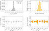 |
Fig. C.1 Force and energy prediction errors for the test set (16% of the dataset) are summarized across different molecular systems. The upper plots highlight overall errors, while in the lower section, violin plots show the distribution of errors in both forces (left) and energies (right), grouped by chemical formula. Mean errors for each system are marked to aid comparison. |
Comparison of mean binding energies for CO-W22 binding sites.
 |
Fig. C.2 Distribution of standard deviations of predicted forces (left panel) and energy variances (right panel) for all the binding sites of CO on ASW (npASW and pASW), obtained from three independently trained machine learning potentials derived from the same training dataset. |
Appendix D ASW characterization
Reconstruction of the surface has been carried out using triangulation techniques, where the surface is approximated by a mesh of finite triangular elements. A Triangular 3D Surface Plot (Tri-Surface Plot) is a type of surface plot constructed by triangulating compact surfaces using a finite number of triangles. Each point on the surface lies within one of these triangles. The intersection between any two triangles is either empty, a shared edge, or a shared vertex. The triangulation took into account solely atoms that belongs to the surface of the periodic ice models, based on their Z value. The step size of the grid is 1.5 Å. All surface plots are created using αx.plot_trisurf() function of Matplotlib library(Hunter 2007).
The areal average roughness (S a) of the ASW model is calculated as:
 (D.1)
(D.1)
where Zi are the individual height values,  is the mean height of the surface and N is the number of points. The Mean Roughness Depth (Rz) is calculated as the average of the five largest peak-to-valley differences in the surface:
 (D.2)
(D.2)
where Zmax,j and Zmin,j are the highest and lowest points in each of the five largest peak-to-valley differences. A dangling OH bond, d(OH), is a surface H atom not engaged in any H-bonds with other water molecules. In order to estimate the amount of d(OH) we assumed a threshold of 2.5 Å in the shortest HW1–OW2 distance for two different water molecules W1, W2. The percentage of dangling OH bonds (% d(OH)) is defined as:
 (D.3)
(D.3)
For the 5 npASW and pASW surfaces; where Nd(OH) is the total number of dangling OH and NH is the total number of surface H atoms, estimated excluding bulk H atoms.
 |
Fig. D.1 Left: Top and side view of one of the npASW periodic ice models. Cell dimensions are reported in Å. Oxygen atoms are colored according to their altitude. Hydrogen atoms are colored in red if they are dangling OH bond (i.e. non engaged in any HB-bond), else they are colored in white. Right: analog for one of the pASW ice models. All atoms below the 5.2 or 6.1 Å threshold (for npASW and pASW, respectively) are considered bulk and kept frozen at each stages of the work. |
Appendix E Gaussian bootstrap procedure
To fit a Gaussian curve to the BE distribution taking into account the uncertainty of each binding energy derived from the three MLP models used in the query-by-committee approach, we employed a bootstrap method with 10000 simulations. In our analysis, each BE measurement, xi, is associated with an uncertainty σi that reflects the spread among the three model predictions. We assume that the true value of each measurement is normally distributed about xi with variance  :
:
 (E.1)
(E.1)
In each bootstrap simulation, we generate perturbed data by adding Gaussian noise to each measurement:
 (E.2)
(E.2)
For each simulation, we compute the sample mean and sample standard deviation:
 (E.3)
(E.3)
 (E.4)
(E.4)
where Ndata is the number of measurements. This procedure is repeated N = 10000 times. The final estimates for the mean and standard deviation are then obtained as the averages over the simulations:
 (E.5)
(E.5)
The uncertainties in these estimates are given by the standard deviations of the corresponding bootstrap distributions:
 (E.6)
(E.6)
The Gaussian probability density function is defined as
 (E.7)
(E.7)
To quantify the uncertainty in the histogram of the BE distribution, we compute error bars for each histogram bin based on the bootstrap simulations. Let ni,j denote the count in the i-th bin for the j-th bootstrap simulation, with j = 1,…, N. The mean count in bin i is given by
 (E.8)
(E.8)
where N = 10000 and the error bar for bin ¡, representing the uncertainty in the count due to the propagated measurement errors, is calculated as
 (E.9)
(E.9)
This approach propagates the individual uncertainties from the neural network models into the Gaussian fitting procedure.
Appendix F Interaction energy incremental analysis
We examined how the different contributors to the interaction energy converges in relation to the size of the binding sites, for two VH-BE example structures belonging to different classes, also reported in Fig. 5. Fig. F.2 illustrates the results as the binding site expands from 2 to 35 water molecules around the CO adsorption location, in the stationary-point geometry. The 0 K baseline corresponds to the original energy value for the CO−W35 structures, such that the plotted energies represent the deviation at each cluster size. For both structures, the largest attractive contribution to the interaction energy comes from the dispersion, followed by electrostatic and induction energy, while the only repulsive interaction corresponds to the exchange energy.
For the Elst-class structure, upper panel, all the contributes are converged within the first 10 water molecules. This confirms the rather local character of the primarily electrostatic interaction between CO and the ASW surface, as recovering the full interaction energy requires only a small portion of the water molecules near the binding site. On the other hand, for the Disp-class structure, lower panel, the dispersion energy contribution is the slowest to converge, as expected, and reaches full convergence when the binding site has grown to ~ 20 water molecules. Moreover, al contributions to the interaction energy are larger than the El-structure, which is consistent with a CO molecule further embedded into the ASW H-bond network.
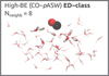 |
Fig. F.1 Example of Very High (VH)-BE structure belonging to ED-class (BE = 1630 K). The figure displays a portion of the binding site comprising 50 water molecules, represented as sticks. The water molecules within 4.5 Å of CO center of mass (i.e. nearest neighbors) have been highlighted. |
 |
Fig. F.2 Convergence of SAPT0-D3MBJ interaction energy components for CO as a function of binding site size. The plot is generated by incrementally adding water molecules to CO from an extracted VH-BE Elst-class binding site (upper panel) and a VH-BE Disp-class binding site (lower panel). The interaction energy difference are with respect of the CO + W35 limit (∆Eint = Eint(CO + W35) − Eint (CO + WX). The interaction energy in the Elst-class converges significantly faster than in the Disp-class binding site. The interaction energy is further decomposed into electrostatic, induction, dispersion and exchange contribution, of which the dispersion interaction is the slowest to converge. Therefore, selecting a binding site extract comprising 28 water molecules captures almost the totality of the interaction energy of CO + ASW. |
Appendix G Simulated TPD curve generation
The simulated temperature-programmed desorption (TPD) traces were generated based on a first-order desorption model.
Desorption rates for each population were computed using a first-order Arrhenius expression:
 (G.1)
(G.1)
with v as the pre-exponential factor (s−1).
In order to simulate the temperature evolution during a TPD experiment, we used a linear heating ramp:
 (G.2)
(G.2)
with T0 as the initial temperature and β as the heating rate (K/s). Surface coverage θi·(t) for each population was obtained by integrating the differential equation:
 (G.3)
(G.3)
In order to consider the complete BE distribution, it was dis-cretized into 40 bins. For each bin, the bin center is taken as the representative binding energy, Ei, and the weight for that bin is computed as follows. If ni is the number of states falling into the ith bin, then the weight is defined as
 (G.4)
(G.4)
so that the weights satisfy
 (G.5)
(G.5)
On the other hand, the instantaneous desorption flux from each population is given by:
 (G.6)
(G.6)
The individual fluxes are summed to yield the overall TPD signal:
 (G.7)
(G.7)
Furthermore, in TPD experiments, CO molecules initially bound to low BE sites often diffuse to higher BE sites before desorption. To more accurately reflect this phenomenon, we applied minimum BE cutoffs. This approach considers only desorption events originating from sites with BE values exceeding the cutoff, effectively mimicking the observed migration and subsequent desorption from higher BE sites in real TPD scenarios Hence, for each cutoff, only sites with E ≥ Emin were retained. To consider the lowering in surface coverage, initial coverage θ0 was scaled by the fraction f of states surviving the cutoff:
 (G.8)
(G.8)
where Nfiltered is the number of states remaining after the cutoff, and Nall is the total number of states. Increasing the cutoff reduces the effective initial coverage, resulting in desorption peaks shifting to higher temperatures and lower integrated TPD signals. This approach effectively captures the desorption dynamics arising from discrete adsorption populations and surface diffusion effects.
The heterogeneous nature of interstellar grain surfaces in astrochemical models is an active area of research; see, e.g., Molpeceres et al. (2024); Kalvans etal. (2024).
All Tables
Interaction energies (IE) obtained at the different symmetry-adapted perturbation (SAPT) flavors.
Focal point analysis in kcal mol−1of the binding energy for the CO − W2 − b structure.
Focal point analysis in kcal mol−1of the binding energy for the CO − W3 − a structure.
Focal point analysis in kcal mol−1 of the binding energy for the CO − W3 − b structure.
Focal point analysis in kcal mol−1 of the binding energy for the CO − W3 − c structure.
Interaction energy, deformation energy, and binding energy at the CCSD(T)/CBS level of theory.
RMSD for the binding site geometry of the CO − W2 − b and CO − W3 − b structure with different hybrid and metahybrid DFT functionals.
Mean absolute error (MAE) in K of binding energies for benchmarked DFT functionals.
Binding energy and ZPVE values obtained at the CCSD(T)-F12/cc-pVDZ level of theory.
Training set composition and test set accuracy for the machine learning potential.
All Figures
|
Fig. 1 Model systems of CO–W2–3 used for the DFT energy and geometry benchmark. Rows show structure names and binding energies (BE). Numbers in parentheses indicate the ZPVE-corrected BE value. The water molecule acting as the H-bond donor to CO is labeled WD. Characteristic distances are given in Å; energy values are in K. Atoms are color coded as follows: black for C, red for O, and white for H. |
| In the text | |
|
Fig. 2 Upper panel: top view of one of the nonporous (npASW) (left) and porous (pASW) ice models. Each periodic surface contains 500 water molecules. Lower panel: altitude plot relative to the same two structures (see Appendix D). Periodic cell dimensions are indicated. Distances are given in Å. |
| In the text | |
|
Fig. 3 Histograms of the ZPVE corrected BEs obtained for CO adsorbed on five npASW (upper panel) and five pASW surfaces (lower panel). The color-coded bars below each panel indicate the BE groups (VL: Very Low, Low, Medium, High, and VH: Very High). Gaussian fits were obtained using the bootstrap procedure detailed in Appendix E, which propagates individual uncertainties from the neural-network models into the Gaussian fitting procedure. |
| In the text | |
|
Fig. 4 CO-npASW panel showing (left) BE distribution for CO on npASW ice, with color mapping highlighting the dominant interaction contributions at various binding sites, ranging from primarily electrostatic (Elst-class, blue) to purely dispersion (Disp-class, orange), while ED-class (gray) represents an intermediate group. The coefficient that determines the class of a binding site is the ratio between the dispersion energy and the sum of the attractive interaction energies (electrostatic, induction, and dispersion), as defined in Sect. 2.2. (Right) Correlation between the BE and CO number of neighbors (i.e., the number of water molecules within a radius of 4.5 Å of the CO center of mass) for each class of binding sites. Averages are shown as points connected by a dashed line, and the standard deviation is shown as a shaded region of matching color. CO-pASW panel: Analogous data for pASW ice. |
| In the text | |
|
Fig. 5 Example of Very High (VH)-BE structures belonging to the Elst-class (blue, BE = 1370 K) and Disp-class (orange, BE = 1492 K), and their location on the pASW surface, represented as an altitude map. The inset figures display a portion of the binding sites comprising 50 water molecules, represented as sticks. Water molecules within 4.5 Å of the CO center of mass (i.e., nearest neighbors, Nneighb) are highlighted. |
| In the text | |
|
Fig. 6 Simulated TPD traces using BE distributions from our study compared to different experimental results of multicoverage TPD desorption from Noble et al. (2012b), Nguyen et al. (2018), and He et al. (2016). The heating ramp rate (β) is 0.3 K s−1 (See Appendix G for further details). Different colored TPD traces correspond to simulations considering different BE cutoffs in the distribution, excluding BEs lower than min(BE)(see Table 3). The initial coverage for each TPD trace corresponds to the fraction of molecules of the full distribution remaining after applying the cutoff. The shaded area represents the range of experimental TPD results. Two pre-exponential factors are shown: v = 1012 s−1 (solid lines) and v = 9.14 × 10¹⁴ s−1 (dashed lines), the latter is derived from transition state theory as detailed in Minissale et al. (2022). |
| In the text | |
|
Fig. 7 Two dimensional spatial distributions of CO gas (upper panels) and ice (lower panels) abundances on the disk, shown using a multibinding description (left panels) and a single binding description (right panels). The vertical axes represent height normalized by radius. Dashed lines depict the positions where the dust temperature is equal to 30, 25, 15, and 10 K. |
| In the text | |
|
Fig. 8 Vertically integrated CO gas and ice column densities as functions of radius. The left panel shows the model with the multibinding description, while the right panel shows the single binding description. |
| In the text | |
|
Fig. C.1 Force and energy prediction errors for the test set (16% of the dataset) are summarized across different molecular systems. The upper plots highlight overall errors, while in the lower section, violin plots show the distribution of errors in both forces (left) and energies (right), grouped by chemical formula. Mean errors for each system are marked to aid comparison. |
| In the text | |
|
Fig. C.2 Distribution of standard deviations of predicted forces (left panel) and energy variances (right panel) for all the binding sites of CO on ASW (npASW and pASW), obtained from three independently trained machine learning potentials derived from the same training dataset. |
| In the text | |
|
Fig. D.1 Left: Top and side view of one of the npASW periodic ice models. Cell dimensions are reported in Å. Oxygen atoms are colored according to their altitude. Hydrogen atoms are colored in red if they are dangling OH bond (i.e. non engaged in any HB-bond), else they are colored in white. Right: analog for one of the pASW ice models. All atoms below the 5.2 or 6.1 Å threshold (for npASW and pASW, respectively) are considered bulk and kept frozen at each stages of the work. |
| In the text | |
|
Fig. F.1 Example of Very High (VH)-BE structure belonging to ED-class (BE = 1630 K). The figure displays a portion of the binding site comprising 50 water molecules, represented as sticks. The water molecules within 4.5 Å of CO center of mass (i.e. nearest neighbors) have been highlighted. |
| In the text | |
|
Fig. F.2 Convergence of SAPT0-D3MBJ interaction energy components for CO as a function of binding site size. The plot is generated by incrementally adding water molecules to CO from an extracted VH-BE Elst-class binding site (upper panel) and a VH-BE Disp-class binding site (lower panel). The interaction energy difference are with respect of the CO + W35 limit (∆Eint = Eint(CO + W35) − Eint (CO + WX). The interaction energy in the Elst-class converges significantly faster than in the Disp-class binding site. The interaction energy is further decomposed into electrostatic, induction, dispersion and exchange contribution, of which the dispersion interaction is the slowest to converge. Therefore, selecting a binding site extract comprising 28 water molecules captures almost the totality of the interaction energy of CO + ASW. |
| In the text | |
Current usage metrics show cumulative count of Article Views (full-text article views including HTML views, PDF and ePub downloads, according to the available data) and Abstracts Views on Vision4Press platform.
Data correspond to usage on the plateform after 2015. The current usage metrics is available 48-96 hours after online publication and is updated daily on week days.
Initial download of the metrics may take a while.