| Issue |
A&A
Volume 703, November 2025
|
|
|---|---|---|
| Article Number | A99 | |
| Number of page(s) | 15 | |
| Section | The Sun and the Heliosphere | |
| DOI | https://doi.org/10.1051/0004-6361/202555839 | |
| Published online | 10 November 2025 | |
Solar flare forecasting utilizing deep survival analysis
Probabilistic time-to-event analysis
Astronomical Institute (AIUB), University of Bern, Sidlerstrasse 5, CH-3012 Bern, Switzerland
⋆ Corresponding author: This email address is being protected from spambots. You need JavaScript enabled to view it.
Received:
6
June
2025
Accepted:
19
September
2025
Abstract
Context. Solar flares and their associated particle ejections can have adverse effects on technology on Earth. Solar flare forecasting, the prediction of such high-energy outbursts on the Sun, is becoming increasingly important as space missions and infrastructure expand. To enhance the prediction of flare timing, we combined survival analysis, traditionally used in medicine, with deep learning.
Aims. Our objective is to improve flare prediction by eliminating fixed time decision boundaries during model training. This allows the model to capture the evolving flare risks within solar active regions. The aim is to further integrate a discrete classifier that triggers warning systems based on the underlying continuous time-to-event predictions.
Methods. We employed deep survival analyses to estimate the likelihood and timing of a flare using photospheric vector magnetogram data from solar active regions. Deep survival analysis estimates the probability of an event occurring over time, in our case the next flare. A subsequent step utilizes a support vector machine (SVM) to provide discrete warning classifications on a flexible time decision boundary.
Results. Our survival model effectively predicts time-to-event survival probabilities, following the evolution of active regions and capturing temporal data patterns. With an averaged true skill statistic (TSS) of 0.71 across classes, the SVM distinguishes between low-risk, future, and imminent flare events. Nonflaring regions are well separated with a TSS of 0.84, while differentiating between short- and long-term flare predictions is more challenging, with TSS scores ranging from 0.3 to 0.7 depending on warning thresholds of 8 to 60 hours.
Conclusions. By removing rigid time boundaries, our continuous-time survival analysis approach enhances real-time forecasting capabilities and addresses the limitations of traditional models. Future studies may further refine and optimize these techniques.
Key words: methods: data analysis / methods: statistical / Sun: activity / Sun: flares
© The Authors 2025
 Open Access article, published by EDP Sciences, under the terms of the Creative Commons Attribution License (https://creativecommons.org/licenses/by/4.0), which permits unrestricted use, distribution, and reproduction in any medium, provided the original work is properly cited.
This article is published in open access under the Subscribe to Open model. This email address is being protected from spambots. You need JavaScript enabled to view it. to support open access publication.
1. Introduction
Solar flares are intense bursts of electromagnetic radiation that are able to eject billions of particles into interplanetary space and toward Earth. Both radiation and energetic charged particles can damage satellite electronics, while the latter are also able to disrupt air traffic communication and navigation when they breach the Earth’s magnetic field. In severe cases, currents may be induced in local power grids, damaging them or even leading to a complete shutdown (Boteler 2001; Pulkkinen et al. 2005; Krausmann et al. 2014). Despite the great deal of interest in predicting solar flares, models are still not fully able to make adequate forecasts, due to the complex underlying physical processes.
While studies on flare precursors in the solar atmosphere are ongoing (Li et al. 2020; Panos et al. 2023; Zbinden et al. 2024), studies on flare forecasting consistently highlight the strong connection between solar flares and the strength and configuration of the magnetic field, spanning from the photosphere to the corona (Leka & Barnes 2003, 2007; Welsch et al. 2009; Sun et al. 2023). Key precursors include increases in magnetic helicity (Leka & Barnes 2003, 2007; Georgoulis et al. 2009) and flux across high-gradient active region polarity inversion lines (Schrijver 2007; Bobra & Couvidat 2015). Many forecasting models thus lean on quantities extracted from magnetograms or extreme ultraviolet (EUV) emissions (Sun et al. 2023; Francisco et al. 2024).
The prediction of solar flares is predominantly approached as a binary classification problem, distinguishing between flaring and nonflaring events based on a specific point in time as the decision boundary (Bobra & Couvidat 2015; Nishizuka et al. 2018; Liu et al. 2019; Deng et al. 2021; Sun et al. 2022; Abduallah & Wang 2024, among others). While binary classifiers can provide predictions for these single predetermined durations, the interpretability and flexibility provided by modeling the event probabilities as a function of time can be lost. Multi-class classification approaches (e.g. Chen et al. 2019; Jiao et al. 2020) are one way to remedy this loss of information. However, since the problem is still posed as a binary classification problem, and the employed machine learning models are exclusively trained as such, the time-to-flare prediction is only imitated by multiple decision boundaries.
Other authors have tried to tackle the continuity problem with the approach of waiting time statistics, where the probability density function of waiting times, the interval between two successive events, is analyzed with the aim of understanding temporal patterns such as whether these intervals follow a Poisson process, power law, or other statistical distribution (Li et al. 2018; Nurhan et al. 2021; Aschwanden et al. 2021). While this approach provides insights into flare recurrence, it fundamentally relies on fitting observed intervals to theoretical distributions, which limits its predictive power, particularly for the initial flare or events in dynamically evolvingconditions.
To model continuous event probabilities, studies in other fields of research have used marked temporal point processes (Daley & Vere-Jones 2007; Mei & Eisner 2017; Gupta et al. 2022), continuous-time Markov chains (MacDonald & Pienaar 2023; Reeves & Bhat 2023), or other machine learning architectures based on statistics and nonlinear regression (e.g. Shain 2021; Shain & Schuler 2024). In our study we decided to employ the most widely used deep survival analysis method based on Cox (non)proportional hazard regression (Cox 1972; Faraggi & Simon 1995; Katzman et al. 2018; Kvamme & Borgan 2021), which completely removes classification boundaries. This provides a new avenue for flare prediction using continuous-time labeling (see Sect. 2) without the need for predefined starting points. Thus far, this method has primarily been used in the fields of medicine and reliability engineering (Chaddad et al. 2023; Wiegrebe et al. 2024; Zapletal 2025), for example estimating the risk of mortality in patients with heart failure (Ahmad et al. 2017) or forecasting equipment failures to support predictive maintenance in industrial settings (Li et al. 2022).
2. Methodology
Given that survival analysis is a novel approach to solar flare forecasting, we begin with a short introduction to its theoretical principles. We closely follow the derivations that have been explicated in other works (Katzman et al. 2018; Kvamme & Borgan 2021; Li et al. 2022; Zhong et al. 2021; Wiegrebe et al. 2024).
The object of survival analysis is to model the probability of an event as a continuous function of time. Let T be a random variable that denotes the time of such an event. The cumulative distribution function of T is given by FT(t) = P(T ≤ t), where P(T ≤ t) is the probability that the event T happens before or at time t. We define the survival function ST as
 (1)
(1)
which, in classical survival analysis, describes the probability of surviving beyond time t. In the case of solar flare forecasting, this would translate to the probability that a flare has not yet happened at time t.
Instead of working with the survival function directly, the usual approach models the hazard rate hT(t) as
 (2)
(2)
where fT(t) is the probability density function of the random variable T. The hazard rate describes the instantaneous risk of the event occurring in an infinitesimal interval after time t, given it has not yet occurred at time t. Following Equations (1) and (2), we can express the hazard rate as
 (3)
(3)
Solving for the survival function, we obtain
 (4)
(4)
where the integral in the exponential is typically called the cumulative hazard H(t).
One of the most common models for the hazard rate is the Cox proportional hazard model (CoxPH), which models the hazard rate based on features X and parameters β as the product of a nonparametrically estimated baseline hazard h0(t) and an exponential risk based on a predictor θ (Cox 1972):
 (5)
(5)
The proportionality of the model arises from the time dependence, which is encapsulated only in the baseline hazard. Thus, the ratio of hazard rates based on two sets of features, X1 & X2, will be constant in time, as the baseline hazard cancels out. This proportionality assumption can be highly restrictive, especially when trying to model complex and dynamic systems such as active regions on the Sun, as well as the occurrence of flares. We therefore include a time dependency also in the exponential risk as proposed by Kvamme & Borgan (2021),
 (6)
(6)
and treat time as an additional feature in the partial hazard, leading to the Cox nonproportional hazards model. This is much more computationally expensive as we need to compute θ(t|X) for all distinct event times Ti ≤ t. However, with this, a sufficiently complex model can include interactions, stratification, and nonlinear and time-varying effects. The model is tuned by maximizing the Cox partial likelihood Lcox, which we introduce in the following paragraph.
Let X1, X2…,Xn denote the covariates of the total data-population N = {1, 2, …, n}. The probability that the first event occurs with covariates X1 and event-time T1 is given by
 (7)
(7)
By multiplying the likelihoods for following events, we get the total likelihood that the sequence of events is T1, T2, …, Tn:
 (8)
(8)
Here i : Ci = 1 denotes all elements of N that will experience an event. The remaining data population that is not associated with any event gets assigned an event indicator of Ci = 0. Furthermore, we define the risk set ℛi of event Ti as ℛi = {Xn : Tn ≥ Ti | n ∈ N}, representing the set of all features with associated event-times after time Ti.
In our analysis, some time series exhibit exceptionally long durations, extending to 10 days or more. To address this, we apply censoring, a characteristic aspect of survival analysis, which involves setting a maximum time Tmax as an upper cutoff, such that T = min(Ti, Tmax). In classical survival analysis, the cutoff does not need to be constant but can be individual for each flaring or nonflaring data series. By virtue of our data, Tcensored = Tmax = const. Whenever we need to apply the censoring to a set of features, we mark them with the indicator Ci = 0.
In the application of deep survival analysis, the model function θ gets replaced by a neural network that has a single node output estimate,  , based on a parameterization β. This parameterization is chosen such that it minimizes the loss function given by the negative partial log-likelihood, derived from the Cox likelihood (8),
 (9)
(9)
Once we find the parameter set β that minimizes the loss function given by Eq. (9), we can obtain predictions by estimating the survival function (4),  . In practice, the cumulative hazard
  is estimated by
 (10)
(10)
where  is an increment of the Breslow estimator (Cox 1975; Lin 2007), specifically
 (11)
(11)
3. Data and event selection
We used the Space Weather Analytics for Solar Flares (SWAN-SF) dataset (Angryk et al. 2020) for the training of our model. This dataset is a partitioned collection of multivariate time series extracted from solar photospheric magnetograms in the Spaceweather HMI Active Region Patch (SHARP) series (Bobra et al. 2014; Angryk et al. 2020). The Helioseismic and Magnetic Imager (HMI) (Schou et al. 2012), is an instrument on board the Solar Dynamics Observatory that observes the photospheric Fe I absorption line at 6173 Å. This dataset was specifically designed for machine learning tasks and is widely used in the community. The time series has a cadence of 12 minutes and spans periods with active regions during the time period from May 2010 to December 2018. In the original dataset, each series was divided into k equal-length slices. The (i + 1)th slice begins at si + τ, where si is the start time of slice i and τ a step size of 1 hour. The final slice ends at the time of the associated flare occurrence or, for nonflaring active regions, at the end of the observation window. However, in our case, slicing and temporally overlapping series are unnecessary, so we concatenate the segments into one sequence per flare.
In addition to features based on magnetograms, such as the total unsigned current helicity or the total magnitude of the Lorentz force, the SWAN-SF dataset includes the maximum of one-minute averaged X-ray flux data during the 12-minute interval. We used images from the Atmospheric Imaging Assembly (AIA, Lemen et al. 2012) 171 Å channel to visually compare our results with the observed evolution of an active region.
First tests in the application of survival analysis demonstrate that working with a preprocessed version of the SWAN-SF dataset significantly improved model stability and performance by up to 40%. Following a similar approach to Hostetter et al. (2019), we compute running summary statistics over a 4-hour window for each extracted magnetogram feature to produce more consistent and reliable inputs for our survival model. These statistics are computed at the same 12-minute cadence as the SWAN-SF dataset.
Labeling for a set of statistics i is done by using the event indicator Ci and time-to-event T = min(Ti, Tmax), where the censoring time Tmax is set to 6 days. A value for Tmax of 6 days represents the 90th percentile time-to-event of all flaring observations and encompasses the main build-up phase to a flare, generally found to be 1−3 days (Tian & Liu 2003; Toriumi & Wang 2019; Liu et al. 2025), in addition to leaving room for a previous growth-phase, capturing long-term gradual build-up behavior and evolution. Using the 90th percentile as cutoff ensures that our data also includes active regions which will flare in the future, bridging the gap between flare-imminent time series and never-flaring time series. In this setting, we define an event to be an ≥M flare. C, B, and A flares are all considered nonflaring in the context of event labeling. The full list of statistical quantities calculated on each feature is provided in Table 1, including features that focus on long-term trends.
Statistical features X1, …, Xp calculated for each extracted magnetogram feature Y of the SWAN-SF dataset.
Previous studies found that one of the major indicators for future flares is the flare history of an active region, that is, the frequency and timing of prior flares (e.g. Nishizuka et al. 2017), as analyzed in approaches using waiting time statistics (cf. Sect. 1 and references therein). Similar to the original structure of the SWAN-SF dataset, our time series for flaring active regions are split by the occurrences of M and X flares in that region. This means that each endpoint of a flare-associated time sequence is the point in time when the GOES X-ray flux emergent from the considered active region reaches a threshold of 10−5 W/m2. While this approach allows us to cleanly separate flares, we lose the information about previous events. However, in order to include a notion of flare history, we include occurrences and intensity of B and C flares in the statistical running-window time series. This is accomplished by adding two additional features – one for B-class flares and one for C-class flares – representing the total count of flares in each category within the window and their summed intensities.
Furthermore, our model takes as a categorical input feature the flare class to expect: None, M1.0, M1.1, …, X9.9. Of course, this information is not available for new flares that one tries to predict. We therefore apply a random forest classification (RFC) on test data prior to passing them to the trained deep survival model and obtain an estimate of the expected flare class. We do not aim to perfectly capture the challenging task of classifying future flares with the RFC, but only to get a rough estimate of what might be the intensity range of an upcoming flare. More details on this are given in Sect. 4.
Combining statistical features with the B- & C-flare history and approximated flare intensity, we get a total number of 579 features as input for our model.
The commonly pursued task of separating M and X class flares from C, B, and A flares, as well as flare-quiet active regions, relies on careful treatment of data imbalances. Depending on the partition, these imbalances range from 1:20 up to 1:95 (Angryk et al. 2020; Ahmadzadeh et al. 2021). Moreover, the total amount of data associated with a single flare can vary significantly: the first flare in an active region typically has a long time series, while subsequent flares are preceded by much shorter time series.
To address these imbalances, we employ a combination of under- and oversampling techniques, guided by four key considerations: (i) flare types become less frequent with increasing intensity, and some may be underrepresented in the dataset; (ii) active region time series vary in length; (iii) flare time series are generally shorter than nonflaring time series; and (iv) we aim to include time series extending beyond the censoring time of Tmax. To mitigate (i), we oversample active regions that experience underrepresented events (e.g., M1.5 flares) in the SWAN-SF dataset using kernel density estimations (KDEs). Underrepresented flares are duplicated until their counts align with the KDE. As nonflaring active regions are more prominent in the dataset, we undersample associated data to prevent event times Ti → ∞ (treated as censored at Tmax) from dominating the time-to-event distribution (Fig. 3). We opt to reduce the total number of nonflaring active regions, instead of truncating flare-quiet time series, to ensure compliance with (iv). We do so by randomly choosing nonflaring active region time series until we reach the data count of the flaring majority class, M1.0.
The final dataset distribution with regard to flare type and time-to-event, respectively, can be seen in Figs. 2 and 3. Examples of flares, minor flares (i.e., B- and C-flares), as well as flare-quiet active regions contained in our dataset are depicted in Fig. 1.
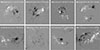 |
Fig. 1. Images from HMI of active regions contained in the dataset that are considered as flaring (upper row) and nonflaring (lower row) by the applied classification scheme of separating M- and X-class flares from the rest. FQ refers to a completely flare-quiet region. |
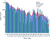 |
Fig. 2. Data count distribution after over- and undersampling in active region and flare type data. Nonflares are labeled “−1”. In red, we plot the KDE used for oversampling. |
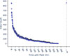 |
Fig. 3. Data counts of flare times. We note the right end of the distribution, which is associated with flare-quiet active regions. Any event-time above 6 days (144 hours) is treated as censored (see Sects. 2 and 3). |
4. Model and neural network
In our study, we utilize an implementation of a mixed-input multi-layer perceptron (MLP) in order to replace the log partial hazard θ in Eq. (6) by a neural network θNN. The MLP is a supervised machine learning algorithm that has its roots in the works of Rosenblatt (1957) and Rumelhart et al. (1986, 1988) and constitutes one of the backbones of modern deep learning. Its goal is to learn a function θNN : ℝm → ℝn by training on a dataset, where m is the number of dimensions for the input (features) and n the number of dimensions for the output (target). Given a set of features and a target, the neural network can learn nonlinear relationships for classification or regression tasks, using backpropagation and a parameter optimizer such as gradient descent or Adam (Kingma & Ba 2014). In between input and output layers, there can be one or multiple connected nonlinear layers, called hidden layers, with trainable weights and biases. In the present case, our model consists of 6 layers with 26…21 neurons, chosen based on experimentation.
For each training epoch, batches of 150 prepared feature sets and their time-to-flare are passed to the model. Nonflaring active regions are assigned a censored flare time of Tmax equal to 6 days, while also flagging them as nonflaring with C = 0 when calculating the loss function described by Equation (9). The parameter Tmax can be considered as a configuration parameter of the network (a so-called hyperparameter), but also as a flexible way to define at which maximum timescales we want to analyze an active region.
In addition to the features described in Table 1, the mixed-input MLP takes in occurrences of B and C flares during the 4-hour running-statistics time window, as well as the flare type, as categorical features, described in Sect. 3. Because the flare type is not known for new data (or the test data), we make use of a random forest classifier based on the concepts of decision tree learning (Breiman 2001), which provides a prediction for the flare type. In a random forest classification, multiple decision trees are created using different random subsets of the data and features. Classifications are done by calculating the prediction for each decision tree and then taking the most popular result (or an average of the results in regression applications). In our case, we use an RFC with 100 decision trees. It is important to emphasize that we do not aim for high performance in evaluating the flare type, but only for a rough first estimate. While the RFC may not be able to predict the precise flare class, it is able to distinguish between nonflaring, M-class, and X-class, with an F1-score1 of 0.85. This categorical feature is passed to the survival model as a proxy for the estimated intensity of a potential outburst. We discuss the sensitivity of the survival model to the RFC prediction in Appendix C.
During fitting of the model we make use of the AdamWR optimizer, a modification of the commonly used Adam optimizer, introduced by Loshchilov & Hutter (2017a). It combines Adam’s ability to adjust the learning rate, which controls the step size used to update model parameters during training, automatically with a technique called warm restarts (Loshchilov & Hutter 2017b). Warm restarts help the model avoid getting stuck in suboptimal solutions by resetting the learning rate, giving the model a chance to explore different parts of the loss landscape. Before each restart, the learning rate is scaled by a factor η, and the time between restarts gradually increases by applying a separate multiplier to the cycle length (time until next restart).
The chosen MLP and optimizer hyperparameter setup is tabulated in Table 2.
Hyperparameter setup for the mixed-input multilayer perceptron θNN ≡ θMLP used as our deep survival network.
The loss function to be optimized is given by Eq. (9). In the case of a big dataset, the risk-set ℛi of an event i (i.e., observations that have not yet experienced a flare before the event time Ti) can become very large, resulting in computationally heavy operations. Thus, we only choose a random subset of the risk-set,  . As noted by Kvamme & Borgan (2021), even using a single-element subset does not degrade the training performance in a significant way. Finding the same conclusion from experiments, we thus adapt a similar approach, only choosing two random elements Xj1, Xj2 of the risk-set ℛi for the calculations in the loss function (9).
The final layout of the training and prediction process is depicted in Fig. 4.
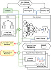 |
Fig. 4. Network diagram. The Cox-survival model, random survival forest, and support vector machines (introduced in Sect. 5.3) constitute the main segments of the overall forecasting model. |
5. Predicted survival
5.1. Evolution of survival functions
For every flare, the output of the model will be a set of survival curves, where every curve belongs to a time step before the flare happens. As we approach the event time, the survival function is expected to decline at a higher rate. An example of such a set of curves can be found in Fig. 6 (middle), where the survival curves start to decline much faster as we approach the flare (colors becoming redder as we approach the flare). That said, the model does not consistently provide clear predictions for all flares (e.g., Fig. 7). To assess the performance of the survival function prediction, we calculate time-dependent receiver operating characteristic (ROCt) curves and their corresponding areas under the curve, AUC(t), using the implementation provided by scikit-survival (Pölsterl 2020). Here, t plays the role of a threshold to distinguish event times T ≤ t and T > t. We expand upon the calculation of these time-dependent metrics in Appendix B. Figure 5 shows that our model is able to achieve AUCt values ranging from 0.72 to ∼0.90 depending on the time threshold t, with a weighted mean of ∼0.75 accounting for data imbalance. This implies that in 72% of cases, a randomly chosen active region that produces a flare by t = 12 h will have a higher predicted risk than a randomly chosen active region that does not experience one by time t = 12 h. For t = 6 days, this increases to a value of 90%.
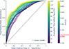 |
Fig. 5. Time-dependent receiver operating characteristic (ROCt) and the respective AUC(t) values for the survival model. As we shift the time threshold t for ROCt calculation, the model’s performance improves, as indicated by the color bars on the right. The data-imbalanced weighted mean AUC reaches a value of 0.751. |
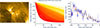 |
Fig. 6. Left: Image of active region AR11169 in AIA channel 171, just before the occurrence of an M4.2 flare on 14 March 2011 (SOL2011-03-14T19:30). Middle: Estimated survival curves as the time series approaches the event (yellow to red). A clear trend is visible, showing the ability of the model to capture the evolving active region before a flare. Right: Mean lifetime curve extracted from the collection of survival curves as we approach the event. The orange curve represents a version of the blue mean lifetime prediction passed through a Gaussian smoothing kernel. The dip around 180 h corresponds to a C6.0 flare. |
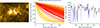 |
Fig. 7. Left: Image of active region AR11432 in AIA channel 171, just before the occurrence of an M2.8 flare on 14 March 2012 (SOL2012-03-14T15:08). Middle: Estimated survival curves as the time series approaches the event (yellow to red). In contrast to the example displayed in Fig. 6, the model is visibly struggling to capture the timing of the flare. Right: Mean lifetimes extracted from the survival curves. There is no visible trend in the results, and outliers and fluctuations are more dominant. This is an example of the model failing. |
Survival functions quantify the probability of a flare happening by each point in time, but they do not directly convey when a flare is most likely to occur. Based on the predicted survival functions, we analyze the mean lifetime as a measure for the expected time to event in the next section.
5.2. Mean lifetime analysis
One way to analyze the time evolution of the prediction is by calculating the mean estimated lifetime for every curve (Hu et al. 2021):
 (12)
(12)
Depending on the computational randomization seed used during data preparation and training, the lifetimes converge toward a common nonzero offset that depends on the seed. This is based on the fact that the Cox model is semi-parametric, i.e., the baseline hazard in Eq. (2) is numerically calculated from the training set. Consequently, the specific flares (and nonflares) included in the training set influence the baseline hazard. We can remove this bias by subtracting the baseline mean lifetime μ0 = ∫0Tmaxexp(−H0(t))dt, where H0(t) is the baseline cumulative hazard following Equations (4) and (12). Additionally, running a Gaussian smoothing kernel over the results allows us to remove prediction inconsistencies and outliers.
This method yields a single prediction curve for each flare, which is no longer restricted by discrete decision boundaries in the time domain but continuous in time. Two such examples are presented in Figs. 6 and 7 (with additional examples in Appendix A). In these figures, the left panels display the active regions observed by AIA 171 Å, the middle panels show sets of survival functions – each curve corresponding to a single time step – and the right panels present resulting mean lifetime prediction curves. The survival functions are color-coded to indicate temporal proximity to the flare: red denotes predictions made closer to the flare, while yellow corresponds to earlier time steps further away from it. In the first example – an M4.2 flare on 14 March 2011 (SOL2011-03-14T19:30; Fig. 6) – time-to-flare prediction exhibits a clear, converging trend as the flare approaches. Multiple B and C flares preceded the main event 2 days before, potentially explaining the early convergence visible in the figure. In contrast, the second example (Fig. 7), an M2.8 flare on 14 March 2012 (SOL2012-03-14T15:08), is not predicted accurately. Remarkably, it appears that in the first example, our model is able to accidentally capture a C6.0 at the beginning of the prediction series.
Figure 8 presents the predicted mean lifetime evolution of an active region that experienced multiple flares (AR12017). Initially, an M2.0 flare occurred, followed by an X1.0 and an M2.1 flare the next day (only predictions for the former are shown in the figure). The figure displays the mean lifetime prediction curves corresponding to the three phases: the period preceding the M2.0 flare, the period preceding the X1.0 flare, and the relaxation phase after the M2.1 flare during which no additional major flares were observed. The model is able to correctly predict the flaring behavior of the active region by first predicting the approach of the M2.0 flare and increasing back to long lifetimes ∼10 hours after the last major flare in the active region occurred. Because the predicted lifetime remains low for most of the intermediate phase, it is difficult to infer the timing of the X1.0 flare, which was the best-observed flare caught by many satellites and telescopes(Kleint 2017).
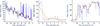 |
Fig. 8. Predicted mean lifetime curves for active region AR12017. Left: Mean lifetime curve for an M2.0 flare on 28 March 2014 (SOL2014-03-28T19:04), the first major flare of the active region. The approach of the flare is clearly visible in the trend of the prediction. Middle: Prediction curve for an X1.0 following the M2.0 flare on the next day (SOL2014-03-29T17:48). The blue curve shows the rapid decrease in lifetime after a few hours, making the timing of the flare difficult to infer. Right: Final part of the series starts on 30 March 2014, where no further major flare occurred. After about 10 hours, the predicted mean lifetime increases, correctly indicating that no further flare will happen. |
For a perfect model, one would expect a linear trend with a slope of magnitude 1 and an intercept of 0 for the lifetime curves, such that  . Figure 9 presents a subset of mean lifetime predictions for various active regions and flare classes. It is evident that, in general, the curves do not follow this expectation. The discrepancy arises because the model is exclusively trained to order flaring times and provide a probabilistic estimate of the likelihood that a flare will occur after a given time. Thus, while allowing us to make continuous time statements about the chance to flare, this approach does not directly offer a way to trigger warning systems based solely on the lifetimes.
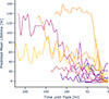 |
Fig. 9. Evolving mean lifetimes for a subset of flares. While most curves converge toward a lifetime of zero, their shapes vary significantly and deviate from an idealized linear model with a slope of one and an intercept of zero. |
Motivated by the deviation from a linear model, we perform an analysis of slopes and average values of linear regressions applied to small intervals within the mean lifetime curve. This is done using a machine learning-based classifier for a specified warning time, such as 24 hours. While this does reintroduce a decision boundary, the warning time remains a continuous free parameter that can be analyzed to gain insights into the timely evolution of the mean lifetime prediction linearity. In the following sections, we detail this procedure and evaluate its performance using various metrics.
5.3. Piecewise linear regressions and support vector machines
To translate mean lifetimes into timely precise warning systems, we analyze the behavior of mean lifetime curves in smaller intervals. This is done by performing piecewise linear regressions on 4-hour windows with 1 hour of overlap between the regression windows.
From these regressions, we derive a new set of features consisting of slopes and mean interval values, which are employed to classify whether a flare will occur within the next x hours, after x hours, or not at all. Using this classification, we can include predictions suitable for triggering warning systems and for reducing the impact of fluctuations in the retrieved mean lifetimes. In addition, these artificially introduced classification boundaries allow us to more directly compare our predictions with conventional forecasting approaches that rely on fixed time boundaries. Nonetheless, a direct comparison of performance with traditional models remains challenging due to the fundamental differences in their underlying modeling processes.
Setting a decision boundary of x = 24 hours, as often used in literature (see references in Sect. 1), we label a set of slope and mean values as flaring within those 24 hours, after 24 hours, or beyond a censoring time of 6 days (potentially never). Given these labels, we train a basic support vector machine classification model (SVM) to distinguish between the three classes. The SVM is a supervised machine learning algorithm based on the hyperplane separation theorem of convex geometry conjectured by H. Minkowski. Its goal is to find a hyperplane (or set thereof) in a higher-dimensional space that best separates one or multiple classes from each other (Boser et al. 1992; Platt et al. 1999). In the present case, these classes are defined as the labels we gave to the sets of slopes and mean values. The multiclass support is handled in a one-vs-one scheme. After training an SVM based on a 24-hour boundary, we shift this boundary to smaller and higher values and re-train the SVM. In this way, we can make use of the time-continuous output of the survival model by setting the time boundary to any value of interest and getting a discrete classification output.
Whilst training the SVM, we ensure that flares belong to the same training or validation group as they belonged to during training of the survival model to prevent leakage between training and testing sets downstream. Furthermore, we cross-validate our results by training a set of 90 models (combined survival model and SVM) based on different data samplings.
5.4. SVM performance metrics
In multi-class classification, each class will be scored individually. However, we can utilize micro-averaging to find a combined score across all three classes. While macro-averaging first computes a performance metric independently for each class and then averages these metrics, micro-averaging will aggregate the contributions of all classes before calculating an average metric. Latter is preferred as we have large class imbalances, which get even more reinforced if we move the time decision boundary from 24 hours to smaller values.
The most common performance metrics calculated for the evaluation of trained classification models are accuracy, precision, and recall. Accuracy is the ratio of the number of correct predictions to the total number of predictions. This metric is often not reliable on its own as it is highly affected by class imbalance. Precision is the proportion of positive cases that were correctly identified, while recall describes the ability of the model to find all of the positive examples (thus also often called sensitivity). Because precision and recall are typically anti-correlated, one often calculates their harmonic mean, called F1-score. Nonetheless, the value that is usually reported and emphasized most is the true skill statistic (TSS, Bloomfield et al. 2012). The TSS is equivalent to one minus the false alarm rate minus the false negative rate. Thus, the best TSS value is 1, and any misclassification, both positive or negative, reduces this score accordingly. Two major advantages of the TSS are that it is (a) typically unbiased with respect to class imbalances and (b) equitable, i.e., a random or constant forecast scores zero and a perfect misclassification −1.
5.5. SVM results
Table 3 summarizes the results over a 24-hour boundary using the metrics introduced in the previous section. The corresponding SVM decision boundaries are shown in Fig. 10. Overall, the model achieves a combined micro-averaged TSS score of 0.71 for the case of a 24-hour decision boundary. By the nature of survival analysis, the model performs best at distinguishing between eventually flaring and nonflaring active regions, with a TSS score of 0.84. Isolating cases in which an active region flares after 24 hours proves to be the most difficult task for the model, only reaching a TSS score of 0.50 and being the primary misclassification category of the other two classes. The SVM achieves a TSS score of 0.54 for regions flaring within the next 24 hours, primarily struggling to separate from regions flaring after 24 hours. Indeed, taking a look at the primary misclassification category in Table 3, we notice that the SVM has trouble finding a clear hyperplane between these two classes.
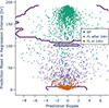 |
Fig. 10. Decision boundaries (green contours) defined by the hyperplanes found by the SVM classification model for a 24 h time boundary that are best at separating the outputs of the linear regression dataset. NF (green dots) constitutes the class representing nonflaring active regions. The NF data points are well separated from the flaring classes (data points in blue and red), whereas the separation boundary for flares occurring within the next 24 hours is more diffuse. |
Performance metrics of the SVM to classify linear regression values as belonging to nonflares (quiet active regions), flares happening in the next 24 hours, or flares happening within the next 24 hours to 6 days.
Figures 11 and 12 illustrate high stability in the overall performance when we shift the temporal prediction boundary. The separation of nonflaring active regions remains consistent for all warning time boundaries, while the flaring decision boundary in data-space shifts as the desired warning time increases. Model performance in separating flaring within the next x-hours and flaring after x-hours is anti-correlated: as the performance improves for the former, it tends to decline for the latter. We find TSS ranging from 0.35 to 0.7 for ‘flaring within the next x-hours’ and 0.6 to 0.3 for ‘flaring after x-hours’, depending on the chosen time boundary.
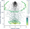 |
Fig. 11. Slopes and mean values of linear regressions computed on overlapping four-hour windows of mean lifetimes retrieved from the survival model, used for the training of support vector machines. We plot a set of decision contours in data space given (arbitrary) time-decision boundaries as targets for the SVMs. As the time boundary increases, the contours deform continuously, demonstrating self-consistency with the shift of boundary. The nonflaring (NF, gray markers) class separation remains similar for every time boundary. The scores for the different boundaries are shown in Fig. 12. |
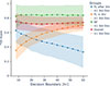 |
Fig. 12. Changes in the average TSS performance on 90 cross-validations (SVM and survival model) as the time decision boundary of the SVM shifts. Decision boundaries close to the flaring time show low scores for the flaring (FL) in x h class due to misclassifications as flaring (FL) after x h. However, as the boundary increases, the scores increase, while the flaring after x h class drops in performance due to misclassifications as nonflaring (NF). The overall (micro-averaged) TSS remains relatively stable at ∼0.71. High scores > 0.8 are consistently achieved for the nonflaring (NF) class, even surpassing 0.9 in certain cross-validation splits. |
6. Discussion
The survival model allows us to remove time boundaries for prediction and provide probabilistic estimations for the time to an event in the form of a mean lifetime prediction. As we approach a flare, these estimations typically approach zero while nonflaring observations retain high mean lifetime estimates.
Generally, we find that mean lifetimes of active regions do not always follow a linear trend in time. This is a further indication of complex physics that can both slowly and rapidly change the dynamics in an active region and trigger solar flares. Further analyzing the mean lifetimes with a support vector machine allows us to partially separate active regions and flares based on the shape of the predicted mean lifetime curve and a target warning time set as a free parameter. Results of the support vector machine demonstrate that our model performs well in separating nonflaring active regions from those that will eventually flare. The implication is that an active region labeled as nonflaring by our model poses very little risk of flaring anytime soon. Even as we shift the time decision boundary, x, which separates the different classes of the SVM, we find that the nonflaring class remains well-separable (see Fig. 11). A similar result is seen in the AUC(t) scores of the survival function estimates themselves, which increase together with the threshold value t from 0.72 to 0.9. While scores for distinguishing between “flaring within the next x-hours” or “flaring after x-hours” are lower, the combined TSS reaches a value of 0.71−0.73. Many other works reach scores of similar magnitude in their respective context. However, since we further process the SWAN-SF dataset and work with statistical quantities, a direct comparison lacks common ground (see Barnes et al. 2016; Leka et al. 2019; Sun et al. 2022). In addition to the difference in dataset, the objective function to be optimized by our model, (9), differs significantly from other works. The same holds true for a potential comparison of AUC(t) scores, presented in Sect. 5.1.
Depending on the data sampling, the performance of the model can vary significantly, as can be seen by the score standard deviation depicted in Fig. 12. Nevertheless, our combined TSS scores are almost constant in time, underlying the fact that we can choose the warning time as a free parameter. The anti-correlated behavior of the score for the flaring classes could potentially be data-driven since the parameter space for “flaring in x-hours” is much smaller than the one corresponding to “flaring after x-hours” for small values of x. Further increasing the dataset, potentially including image data or light-curves, could provide a solution for interpretation and model refinement.
We found that in certain cases, our model is able to capture C flares or general high activity (frequent B and C flares), as in the example outlined in Fig. 6, where a C6.0 flare occurs at the start of the time series, even though the model was not explicitly trained for this task as only ≥M flare were included for training. We, therefore, speculate that classifying predicted flares in a more continuous manner (in contrast to the here applied discrete labeling scheme) might be possible. However, this would likely require significant fine-tuning, and it remains uncertain whether such an approach could yield reliable results.
One example of our model failing is active region AR11432, where our model had difficulty predicting the evolution of survival probabilities prior to an M2.8 flare (see Fig. 7). Overall, the mean lifetime of approximately 26% of all flares does not converge to a value below 10 hours (see Fig. 9 for a subset of flares). The performance of our probabilistic predictions is often difficult to assess in a quantitative way, but in some cases, poor model performance, as in the case of AR11432, can be explained by noticing limb proximity, the presence of other active regions close by (e.g., Fig. A.1), or overall high activity.
Our analysis reveals that our model is particularly well-suited for predicting the first flare in an active region. This predictive strength arises because the first flare is typically preceded by a more extensive time series that captures the dynamic evolution of the region. In contrast, the time series for subsequent flares are typically short and accompanied by additional B- and C-flares, which results in consistent low lifetime predictions. Although low values indicate that another flare will happen, their lack of variation means the model is less effective at pinpointing the specific timing of later flares in the same active region and thus negating many of the advantages of our approach (see e.g., Fig. 8). Therefore, we believe a combination with other forecasting models that better perform on consecutive flares could be the key to improving flare prediction capabilities even further.
Because our model relies on statistical features calculated over a 4-hour window of data extracted from SHARP parameters, a minimum of 4 hours of observations is required in an operational context to generate a single survival curve and mean lifetime estimate. Once this threshold is met, the SVM algorithm can be applied if discrete classifications based on a warning time are desired. However, applying our model to real-time or recent data remains a future step, as this study limits itself to the 2010−2018 period covered by the SWAN-SF dataset.
One question that naturally arises is the matter of interpretability. Although some feature importance studies of the SHARP (and SWAN-SF) parameters for flare forecasting have been done (e.g. Bobra & Couvidat 2015), they were not designed with continuous time-to-event (survival-) analysis in mind. It is plausible that the relevance of magnetic features shifts over time as an active region progresses toward a flare. To investigate this, we are currently exploring frameworks such as SurvSHAP (Krzyziński et al. 2023), which enable time-dependent analyses of feature importance.
7. Conclusion and outlook
This work introduces a novel approach to solar flare forecasting utilizing deep learning time-to-event (survival) analysis on the SWAN-SF dataset extracted from solar photospheric vector magnetogram SHARP series. Our survival model, which is based on Cox nonproportional hazards, can
-
capture the instability of an active region toward a flare by predicting a time-to-event survival probability, translatable into a mean lifetime;
-
remove decision boundaries in the time domain, thus providing a more flexible method than one that depends on a boundary (e.g., 24 hours);
-
capture in-moment activity through fluctuations in the mean lifetime prediction for M- and X-class flares;
-
be assessed by time-dependent receiver operating characteristics and their areas under the curve, AUC(t). In the present case, AUC(t) values fall between 0.72 and 0.9 depending on the value of the time t.
In order to include a method for triggering warning systems for intense outbursts, we have introduced a support vector machine based on piecewise linear regressions of the predicted mean lifetime. The SVM distinguishes between three classes: flaring in x-hours, flaring after x-hours, and nonflaring. The SVM can be adjusted to different decision boundaries in the time domain due to the nature of the preceding survival model. From the SVM we gain the following insights:
-
The averaged TSS of 0.71 over the three classes is independent of the time decision boundary. This demonstrates consistency with the time-continuous output of the survival model.
-
Active regions classified a nonflaring pose very little risk of flaring, as these are well-separable by the SVM at a TSS of 0.84 and the primary misclassification category being flaring after x-hours.
-
Scores for separating flaring in x-hours and flaring after x-hours appear to be anti-correlated and range from 0.35−0.7 and 0.6−0.3, respectively, as we increase the boundary x. This could potentially be data-driven. Nonetheless, it indicates that while general trends in future flare occurrences are well captured, the exact timing is more difficult to predict.
The current state of our model is not yet fully optimized. While we performed a model hyperparameter search for the quantities listed in Table 2, a wide-range parameter search was out of the scope of this paper. Furthermore, the survival model presented in this work utilizes only principal deep learning architectures, such as the multi-layer perceptron, random forest classifier, and support vector machine. A large variety of survival models have been developed in the fields of medicine and economics (cf. Wiegrebe et al. 2024), but not many have been adapted to be used in astrophysics.
This work demonstrates that survival analysis may provide a new avenue to solar flare forecasting, and potentially handling other challenges in solar research that may benefit from a time-continuous prediction, such as lifetimes of coronal holes or of active regions.
Developments in deep survival analysis have introduced various other models such as DeepSurv (Katzman et al. 2018), DeepHit (Lee et al. 2018), tdCoxSNN (Zeng et al. 2024), and ICTSurF (Puttanawarut et al. 2024), which are not only expanding our toolkit for handling complex, nonlinear relationships between covariates and time-to-event predictions, but also addressing traditional limitations related to the loss of information when data are forced into discrete time intervals. Additionally, emerging works involving architectures such as Kolmogorov-Arnold networks (Knottenbelt et al. 2025) and attention-based machine learning models (Hu et al. 2021; Li et al. 2022) explore new ways to capture intricate temporal dynamics within the framework of survival analysis.
In parallel, the integration of explainable AI (XAI) techniques (e.g. Pandey et al. 2023; Panos et al. 2023) into survival analysis may provide new insights into the underlying physics of solar flares. Approaches such as random survival forests (Ishwaran et al. 2008), CoxNAM (Xu & Guo 2023), and post-hoc interpretation tools such as SurvSHAP show promise for integrating interpretability into these models.
We find that a key advantage of survival analysis models is their ability to identify the initial flares of an active region. This suggests that combining survival-based approaches with complementary techniques, such as waiting-time statistics, could offer a promising direction for improving solar flare forecasting even further.
The F1-score is the harmonic mean of precision and recall, where an F1 score reaches its best value at 1 and worst at 0. Metrics are further discussed in Sect. 5.4.
Multiple NOAA numbers are associated: AR11814, AR11816, AR11817, AR11819.
Acknowledgments
This work was supported by an SNSF PRIMA and a SERI-funded ERC CoG grant. We would like to thank every member of the Space Weather group at the Astronomical Institute of the University of Bern for their valuable input and assistance in revising this work, namely Vanessa Mercea, Janis Witmer, Michelle Galloway, Pranjali Sharma, and Dorian Paillon. Our implementation of the survival model makes use of the pycox code, openly available on GitHub (Kvamme et al. 2024).
References
- Abduallah, Y., & Wang, J. T. L. 2024, ArXiv e-prints [arXiv:2405.16080] [Google Scholar]
- Ahmad, T., Munir, A., Bhatti, S. H., Aftab, M., & Raza, M. A. 2017, PLoS ONE, 12, 1 [Google Scholar]
- Ahmadzadeh, A., Aydin, B., Georgoulis, M. K., et al. 2021, ApJS, 254, 23 [NASA ADS] [CrossRef] [Google Scholar]
- Angryk, R. A., Martens, P. C., Aydin, B., et al. 2020, Sci. Data, 7, 227 [NASA ADS] [CrossRef] [Google Scholar]
- Aschwanden, M. J., Johnson, J. R., & Nurhan, Y. I. 2021, ApJ, 921, 166 [Google Scholar]
- Barnes, G., Leka, K. D., Schrijver, C. J., et al. 2016, ApJ, 829, 89 [NASA ADS] [CrossRef] [Google Scholar]
- Bloomfield, D. S., Higgins, P. A., McAteer, R. T. J., & Gallagher, P. T. 2012, ApJ, 747, L41 [CrossRef] [Google Scholar]
- Bobra, M. G., & Couvidat, S. 2015, ApJ, 798, 135 [Google Scholar]
- Bobra, M. G., Sun, X., Hoeksema, J. T., et al. 2014, Sol. Phys., 289, 3549 [Google Scholar]
- Boser, B. E., Guyon, I. M., & Vapnik, V. N. 1992, Proceedings of the Fifth Annual Workshop on Computational Learning Theory, COLT ’92 (New York: Association for Computing Machinery), 144 [Google Scholar]
- Boteler, D. H. 2001, Geophys. Monogr. Ser., 125, 347 [Google Scholar]
- Breiman, L. 2001, Mach. Learn., 45, 5 [Google Scholar]
- Chaddad, A., Hassan, L., Katib, Y., & Bouridane, A. 2023, IEEE J. Transl. Eng. Health Med., 11, 223 [Google Scholar]
- Chen, Y., Manchester, W. B., Hero, A. O., et al. 2019, Space Weather, 17, 1404 [NASA ADS] [CrossRef] [Google Scholar]
- Cox, D. R. 1972, J. Roy. Stat. Soc.: Ser. B (Methodol.), 34, 187 [Google Scholar]
- Cox, D. R. 1975, Biometrika, 62, 269 [Google Scholar]
- Daley, D. J., & Vere-Jones, D. 2007, An Introduction to the Theory of Point Processes: Volume II: General Theory and Structure (Springer Science& Business Media) [Google Scholar]
- Deng, Z., Wang, F., Deng, H., et al. 2021, ApJ, 922, 232 [Google Scholar]
- Faraggi, D., & Simon, R. 1995, Stat. Med., 14, 73 [Google Scholar]
- Francisco, G., Guastavino, S., Barata, T., Fernandes, J., & Del Moro, D. 2024, ArXiv e-prints [arXiv:2410.16116] [Google Scholar]
- Georgoulis, M. K., Rust, D. M., Pevtsov, A. A., Bernasconi, P. N., & Kuzanyan, K. M. 2009, ApJ, 705, L48 [NASA ADS] [CrossRef] [Google Scholar]
- Gupta, V., Bedathur, S., Bhattacharya, S., & De, A. 2022, ACM Trans. Intell. Syst. Technol., 13, 103 [Google Scholar]
- Heagerty, P. J., Lumley, T., & Pepe, M. S. 2004, Biometrics, 56, 337 [Google Scholar]
- Hostetter, M., Ahmadzadeh, A., Aydin, B., et al. 2019, IEEE International Conference on Big Data, 4960 [Google Scholar]
- Hu, S., Fridgeirsson, E., Wingen, G. V., & Welling, M. 2021, Proc. Mach. Learn. Res., 146, 132 [Google Scholar]
- Ishwaran, H., Kogalur, U. B., Blackstone, E. H., & Lauer, M. S. 2008, Ann. Appl. Stat., 2, 841 [Google Scholar]
- Jiao, Z., Sun, H., Wang, X., et al. 2020, Space Weather, 18, e02440 [Google Scholar]
- Katzman, J. L., Shaham, U., Cloninger, A., et al. 2018, BMC Med. Res. Methodol., 18, 24 [Google Scholar]
- Kingma, D. P., & Ba, J. 2014, CoRR, https://api.semanticscholar.org/CorpusID:6628106 [Google Scholar]
- Kleint, L. 2017, ApJ, 834, 26 [Google Scholar]
- Knottenbelt, W., McGough, W., Wray, R., et al. 2025, Bioinformatics, 41 [Google Scholar]
- Krausmann, E., Andersson, E., Murtagh, W., & Mitchison, N. 2014, EGU General Assembly Conference Abstracts, 12584 [Google Scholar]
- Krzyziński, M., Spytek, M., Baniecki, H., & Biecek, P. 2023, Knowledge-Based Systems, 262, 110234 [Google Scholar]
- Kvamme, H., & Borgan, Ø. 2021, Lifetime Data Anal., 27, 710 [Google Scholar]
- Kvamme, H., Hart, B., Pati, S., & Sellereite, N. 2024, pycox (GitHub), https://github.com/havakv/pycox [Google Scholar]
- Lee, C., Zame, W., Yoon, J., & van der Schaar, M. 2018, Proceedings of the AAAI Conference on Artificial Intelligence, 32 [Google Scholar]
- Leka, K. D., & Barnes, G. 2003, ApJ, 595, 1277 [CrossRef] [Google Scholar]
- Leka, K. D., & Barnes, G. 2007, ApJ, 656, 1173 [NASA ADS] [CrossRef] [Google Scholar]
- Leka, K. D., Park, S.-H., Kusano, K., et al. 2019, ApJS, 243, 36 [NASA ADS] [CrossRef] [Google Scholar]
- Lemen, J. R., Title, A. M., Akin, D. J., et al. 2012, Sol. Phys., 275, 17 [Google Scholar]
- Li, C., Zhong, S. J., Xu, Z. G., et al. 2018, MNRAS, 479, L139 [NASA ADS] [CrossRef] [Google Scholar]
- Li, D., Feng, S., Su, W., & Huang, Y. 2020, A&A, 639, L5 [NASA ADS] [CrossRef] [EDP Sciences] [Google Scholar]
- Li, X., Krivtsov, V., & Arora, K. 2022, Reliab. Eng. Syst. Safety, 217, 108033 [Google Scholar]
- Lin, D. Y. 2007, Lifetime Data Anal., 13, 471 [Google Scholar]
- Liu, H., Liu, C., Wang, J. T. L., & Wang, H. 2019, ApJ, 877, 121 [NASA ADS] [CrossRef] [Google Scholar]
- Liu, S., Idrees, S., Liu, D., & Zeng, S. G. 2025, Sol. Phys., 300, 51 [Google Scholar]
- Loshchilov, I., & Hutter, F. 2017a, ArXiv e-prints [arXiv:1711.05101] [Google Scholar]
- Loshchilov, I., & Hutter, F. 2017b, ArXiv e-prints [arXiv:1608.03983] [Google Scholar]
- MacDonald, I. L., & Pienaar, E. A. D. 2023, React. Kinet. Mech. Catal., 136, 1757 [Google Scholar]
- Mei, H., & Eisner, J. M. 2017, Advances in Neural Information Processing Systems (Curran Associates, Inc.), 30 [Google Scholar]
- Nishizuka, N., Sugiura, K., Kubo, Y., et al. 2017, ApJ, 835, 156 [NASA ADS] [CrossRef] [Google Scholar]
- Nishizuka, N., Sugiura, K., Kubo, Y., Den, M., & Ishii, M. 2018, ApJ, 858, 113 [NASA ADS] [CrossRef] [Google Scholar]
- Nurhan, Y. I., Johnson, J. R., Homan, J. R., Wing, S., & Aschwanden, M. J. 2021, Geophys. Res. Lett., 48, e94348 [Google Scholar]
- Pandey, C., Angryk, R. A., Georgoulis, M. K., & Aydin, B. 2023, Discovery Science (Cham: Springer), 567 [Google Scholar]
- Panos, B., Kleint, L., & Zbinden, J. 2023, A&A, 671, A73 [NASA ADS] [CrossRef] [EDP Sciences] [Google Scholar]
- Platt, J., Cristianini, N., & Shawe-Taylor, J. 1999, Advances in Neural Information Processing Systems (MIT Press), 12 [Google Scholar]
- Pölsterl, S. 2020, J. Mach. Learn. Res., 21, 1 [Google Scholar]
- Pulkkinen, A., Lindahl, S., Viljanen, A., & Pirjola, R. 2005, Space Weather, 3, S08C03 [Google Scholar]
- Puttanawarut, C., Looareesuwan, P., Wabina, R. S., & Saowaprut, P. 2024, Inf. Med. Unlocked, 49 [Google Scholar]
- Reeves, M., & Bhat, H. S. 2023, 2023 SICE International Symposium on Control Systems (SICE ISCS), 76 [Google Scholar]
- Rosenblatt, F. 1957, The Perceptron A Perceiving and Recognizing Automaton, Tech. Rep. 85–460-1 (Ithaca, New York: Cornell Aeronautical Laboratory) [Google Scholar]
- Rumelhart, D. E., Hinton, G. E., & Williams, R. J. 1986, Nature, 323, 533 [Google Scholar]
- Rumelhart, D. E., Hinton, G. E., & Williams, R. J. 1988, Readings in Cognitive Science (Morgan Kaufmann), 399 [Google Scholar]
- Schou, J., Scherrer, P. H., Bush, R. I., et al. 2012, Sol. Phys., 275, 229 [Google Scholar]
- Schrijver, C. J. 2007, ApJ, 655, L117 [Google Scholar]
- Shain, C. 2021, Proc. of the 59th Annual Meeting of the Association for Computational Linguistics and the 11th International Joint Conference on Natural Language Processing (Volume 1: Long Papers) (Online: Association for Computational Linguistics), 3718 [Google Scholar]
- Shain, C., & Schuler, W. 2024, Open Mind, 8, 235 [Google Scholar]
- Sun, Z., Bobra, M. G., Wang, X., et al. 2022, ApJ, 931, 163 [Google Scholar]
- Sun, D., Huang, X., Zhao, Z., & Xu, L. 2023, ApJS, 266, 8 [NASA ADS] [CrossRef] [Google Scholar]
- Tian, L. R., & Liu, Y. 2003, A&A, 406, 337 [NASA ADS] [CrossRef] [EDP Sciences] [Google Scholar]
- Toriumi, S., & Wang, H. 2019, Liv. Rev. Sol. Phys., 16, 3 [Google Scholar]
- Welsch, B. T., Li, Y., Schuck, P. W., & Fisher, G. H. 2009, ApJ, 705, 821 [NASA ADS] [CrossRef] [Google Scholar]
- Wiegrebe, S., Kopper, P., Sonabend, R., Bischl, B., & Bender, A. 2024, Artif. Intell. Rev., 57, 65 [Google Scholar]
- Xu, L., & Guo, C. 2023, Expert Syst. Appl., 227, 120218 [Google Scholar]
- Zapletal, D. 2025, Mathematics, 13 [Google Scholar]
- Zbinden, J., Kleint, L., & Panos, B. 2024, A&A, 689, A72 [NASA ADS] [CrossRef] [EDP Sciences] [Google Scholar]
- Zeng, L., Zhang, J., Chen, W., & Ding, Y. 2024, J. Roy. Stat. Soc. Ser. C: Appl. Stat., 74, 187 [Google Scholar]
- Zhong, Q., Mueller, J. W., & Wang, J. L. 2021, Advances in Neural Information Processing Systems (Curran Associates, Inc.), 34, 15111 [Google Scholar]
Appendix A: Further examples
Due to the complexity of the underlying physics, every active region behaves differently in its time-to-event evolution. However, in many cases, these behaviors can be explained by analyzing the active region and its history. In this section, we provide 4 additional explicit examples of different time-to-event evolutions and the output of our model.
On 30 July 2011, an M9.3 flare (SOL2011-07-30T02:04) occurred at active region NOAA AR11261 (SHARP 750). While our model is able to capture the approach of a flare, it overestimates the mean lifetime by approximately 30 hours. Other active regions (AR11263 & AR11260) are close by, potentially increasing the ambiguity of the model. The example is captured in Fig. A.1.
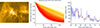 |
Fig. A.1. Left: Image of active region AR11261 in AIA channel 171, close before the occurrence of a M9.3 flare on 30 July 2011 (SOL2011-07-30T02:04). Other active regions (AR11263 & AR11260) are close by, potentially increasing the ambiguity of the model. Middle: Estimated survival curves as the time series approaches the event (yellow to red). A trend is visible. Right: Lifetime showing a decreasing trend starting around 48 hours before the flare. However, at the time of the event, the mean lifetime is still as high as 30 hours. |
On 7 June 2011 a M2.5 flare (SOL2011-06-07T06:16:00) occurred at active region NOAA AR11226 (SHARP 637). This example demonstrates another case in which our model appears to pick up a C8.7 flare (SOL2011-05-29T20:11) at the beginning of the time series. 48 hours before the event, the M2.5 flare is preceded by multiple C1.0 and C1.2 flares, explaining the early convergence toward zero. The example is captured in Fig. A.2.
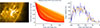 |
Fig. A.2. Left: Image of active region AR11226 in AIA channel 171, close before the occurrence of a M2.5 flare and coronal mass ejection on 7 June 2011 (SOL2011-06-07T06:16). Middle: Estimated survival curves as the time series approaches the event (yellow to red). Due to the high activity and varying lifetimes, the survival curves overlap and are difficult to interpret. Nonetheless, a trend is visible. Right: Mean lifetime curve extracted from the collection of survival curves as we approach the event. This is another example of the survival model accidentally capturing a C8.7 flare (SOL2011-05-29T20:11) at the beginning of the series, similar to the example captured in Fig. 6. The lifetime shows a decreasing trend roughly 5 days before the flare. C1.0 and C1.2 flares, with the addition of 3 B-flares, happened within 48 hours before the main event. |
One example of a nonflaring active region present in the SWAN-SF dataset is the active region with SHARP number 2488 (there is no associated NOAA AR number available). The survival curve evolution is dominated by jumps and fluctuations around 130 to 140 hours in the mean estimated lifetime (close to the censoring time of 6 days). Outliers and fluctuations are removable using Gaussian smoothing. The example is captured in Fig. A.3.
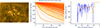 |
Fig. A.3. Left: Image of active region with SHARP-number 2488 (No associated NOAA number provided by JSOC) in AIA channel 171 as an example of a nonflaring active region in February 2013. Middle: Survival curves dominated by fluctuations. No trend is visible. Right: Following the survival curves, the mean lifetime is dominated by large fluctuations. After smoothing with a Gaussian kernel, the curve remains roughly constant at a value of 130 hours (orange line). |
On 12 August 2013, an M1.5 flare occurred at the active region with SHARP-number 3048 (no unique NOAA identifier). The model is able to capture the approach of the flare. Multiple C-flares occurred starting 30 hours before the event, explaining the early convergence of the mean lifetime toward values close to zero. The example is captured in Fig. A.4.
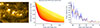 |
Fig. A.4. Left: Image of active region with SHARP-number 30482 in AIA channel 171, close before the occurrence of an M1.5 flare on 12 August 2013 (SOL2013-08-12T10:21). Middle: Evolution of the survival curves showing some minor fluctuations, but the overall trend is clearly visible. Right: Mean lifetimes make the fluctuations in the survival curve evolution clearer. However, Gaussian smoothing is able to remove these variations and extract a clear trend. Regular flares of C-type intensity occur starting ∼30 hours before the M1.5 flare, explaining the early convergence of the mean lifetime toward zero. |
Appendix B: Time-dependent ROC curves for survival analysis
In Section 5.1, we have used time-dependent receiver operating characteristic (ROC) curves and their areas under the curve (AUC) to assess model performance. A ROC curve plots the true positive rate (TPR) against the false positive rate (FPR) over all thresholds θ ∈ ( − ∞, ∞). This results in a monotone increasing function mapping  , where D represents a binary indicator. While in most cases the binary indicator remains constant for each subject, in survival analysis the indicator is a function of time, given as Di(t) = 1 if Ti ≤ t and Di(t) = 0 if Ti > t with Ti being the event (flare) time associated with a set of covariates Xi.
In many adaptations of ROC curves in survival analysis, the TPRt is calculated with the inverse probability of censoring weights retrieved from a Kaplan-Meier estimator fit on the training set (e.g., Heagerty et al. 2004). However, due to the nature of our dataset, these weights collapse to 0 for flare-quiet regions, and those that will only flare after Tmax = 6 days, and to 1 for regions flaring within Tmax days. Considering this simplification, we do not go into further detail on the estimator and the weights. Instead, we refer to the official documentation of the cumulative and/or dynamic AUC of scikit-survival and references therein.
Appendix C: Sensitivity to random forest classification
A random forest classifier (RFC) is included in our model to estimate the potential outburst energy of a flare event. This estimate is then fed into our survival model in the form of another input feature. In order to quantify the impact of the RFC, we fully randomize its estimates in the test set of our model and compare the survival predictions using a set of ROC curves and associated AUC values as done in Sect. 5.1 and explained in Appendix B.
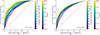 |
Fig. C.1. (a) ROC curves of the data test-set, each associated with a different evaluation time, using a trained RFC for flare-event intensity estimation (flare-class). (b) Similar to (a) but with fully randomized RFC predictions in the test set. |
We find a general decrease in performance of 0.02-0.09, depending on the evaluation time of the ROC or AUC. We further find that the range of achieved AUC values is slightly smaller, and thus less time-dependent. Whether this is an indicator for flare-class-dependent time evolution or not remains speculative. We, therefore, do not further investigate this in the present work.
All Tables
Statistical features X1, …, Xp calculated for each extracted magnetogram feature Y of the SWAN-SF dataset.
Hyperparameter setup for the mixed-input multilayer perceptron θNN ≡ θMLP used as our deep survival network.
Performance metrics of the SVM to classify linear regression values as belonging to nonflares (quiet active regions), flares happening in the next 24 hours, or flares happening within the next 24 hours to 6 days.
All Figures
|
Fig. 1. Images from HMI of active regions contained in the dataset that are considered as flaring (upper row) and nonflaring (lower row) by the applied classification scheme of separating M- and X-class flares from the rest. FQ refers to a completely flare-quiet region. |
| In the text | |
|
Fig. 2. Data count distribution after over- and undersampling in active region and flare type data. Nonflares are labeled “−1”. In red, we plot the KDE used for oversampling. |
| In the text | |
|
Fig. 3. Data counts of flare times. We note the right end of the distribution, which is associated with flare-quiet active regions. Any event-time above 6 days (144 hours) is treated as censored (see Sects. 2 and 3). |
| In the text | |
|
Fig. 4. Network diagram. The Cox-survival model, random survival forest, and support vector machines (introduced in Sect. 5.3) constitute the main segments of the overall forecasting model. |
| In the text | |
|
Fig. 5. Time-dependent receiver operating characteristic (ROCt) and the respective AUC(t) values for the survival model. As we shift the time threshold t for ROCt calculation, the model’s performance improves, as indicated by the color bars on the right. The data-imbalanced weighted mean AUC reaches a value of 0.751. |
| In the text | |
|
Fig. 6. Left: Image of active region AR11169 in AIA channel 171, just before the occurrence of an M4.2 flare on 14 March 2011 (SOL2011-03-14T19:30). Middle: Estimated survival curves as the time series approaches the event (yellow to red). A clear trend is visible, showing the ability of the model to capture the evolving active region before a flare. Right: Mean lifetime curve extracted from the collection of survival curves as we approach the event. The orange curve represents a version of the blue mean lifetime prediction passed through a Gaussian smoothing kernel. The dip around 180 h corresponds to a C6.0 flare. |
| In the text | |
|
Fig. 7. Left: Image of active region AR11432 in AIA channel 171, just before the occurrence of an M2.8 flare on 14 March 2012 (SOL2012-03-14T15:08). Middle: Estimated survival curves as the time series approaches the event (yellow to red). In contrast to the example displayed in Fig. 6, the model is visibly struggling to capture the timing of the flare. Right: Mean lifetimes extracted from the survival curves. There is no visible trend in the results, and outliers and fluctuations are more dominant. This is an example of the model failing. |
| In the text | |
|
Fig. 8. Predicted mean lifetime curves for active region AR12017. Left: Mean lifetime curve for an M2.0 flare on 28 March 2014 (SOL2014-03-28T19:04), the first major flare of the active region. The approach of the flare is clearly visible in the trend of the prediction. Middle: Prediction curve for an X1.0 following the M2.0 flare on the next day (SOL2014-03-29T17:48). The blue curve shows the rapid decrease in lifetime after a few hours, making the timing of the flare difficult to infer. Right: Final part of the series starts on 30 March 2014, where no further major flare occurred. After about 10 hours, the predicted mean lifetime increases, correctly indicating that no further flare will happen. |
| In the text | |
|
Fig. 9. Evolving mean lifetimes for a subset of flares. While most curves converge toward a lifetime of zero, their shapes vary significantly and deviate from an idealized linear model with a slope of one and an intercept of zero. |
| In the text | |
|
Fig. 10. Decision boundaries (green contours) defined by the hyperplanes found by the SVM classification model for a 24 h time boundary that are best at separating the outputs of the linear regression dataset. NF (green dots) constitutes the class representing nonflaring active regions. The NF data points are well separated from the flaring classes (data points in blue and red), whereas the separation boundary for flares occurring within the next 24 hours is more diffuse. |
| In the text | |
|
Fig. 11. Slopes and mean values of linear regressions computed on overlapping four-hour windows of mean lifetimes retrieved from the survival model, used for the training of support vector machines. We plot a set of decision contours in data space given (arbitrary) time-decision boundaries as targets for the SVMs. As the time boundary increases, the contours deform continuously, demonstrating self-consistency with the shift of boundary. The nonflaring (NF, gray markers) class separation remains similar for every time boundary. The scores for the different boundaries are shown in Fig. 12. |
| In the text | |
|
Fig. 12. Changes in the average TSS performance on 90 cross-validations (SVM and survival model) as the time decision boundary of the SVM shifts. Decision boundaries close to the flaring time show low scores for the flaring (FL) in x h class due to misclassifications as flaring (FL) after x h. However, as the boundary increases, the scores increase, while the flaring after x h class drops in performance due to misclassifications as nonflaring (NF). The overall (micro-averaged) TSS remains relatively stable at ∼0.71. High scores > 0.8 are consistently achieved for the nonflaring (NF) class, even surpassing 0.9 in certain cross-validation splits. |
| In the text | |
|
Fig. A.1. Left: Image of active region AR11261 in AIA channel 171, close before the occurrence of a M9.3 flare on 30 July 2011 (SOL2011-07-30T02:04). Other active regions (AR11263 & AR11260) are close by, potentially increasing the ambiguity of the model. Middle: Estimated survival curves as the time series approaches the event (yellow to red). A trend is visible. Right: Lifetime showing a decreasing trend starting around 48 hours before the flare. However, at the time of the event, the mean lifetime is still as high as 30 hours. |
| In the text | |
|
Fig. A.2. Left: Image of active region AR11226 in AIA channel 171, close before the occurrence of a M2.5 flare and coronal mass ejection on 7 June 2011 (SOL2011-06-07T06:16). Middle: Estimated survival curves as the time series approaches the event (yellow to red). Due to the high activity and varying lifetimes, the survival curves overlap and are difficult to interpret. Nonetheless, a trend is visible. Right: Mean lifetime curve extracted from the collection of survival curves as we approach the event. This is another example of the survival model accidentally capturing a C8.7 flare (SOL2011-05-29T20:11) at the beginning of the series, similar to the example captured in Fig. 6. The lifetime shows a decreasing trend roughly 5 days before the flare. C1.0 and C1.2 flares, with the addition of 3 B-flares, happened within 48 hours before the main event. |
| In the text | |
|
Fig. A.3. Left: Image of active region with SHARP-number 2488 (No associated NOAA number provided by JSOC) in AIA channel 171 as an example of a nonflaring active region in February 2013. Middle: Survival curves dominated by fluctuations. No trend is visible. Right: Following the survival curves, the mean lifetime is dominated by large fluctuations. After smoothing with a Gaussian kernel, the curve remains roughly constant at a value of 130 hours (orange line). |
| In the text | |
|
Fig. A.4. Left: Image of active region with SHARP-number 30482 in AIA channel 171, close before the occurrence of an M1.5 flare on 12 August 2013 (SOL2013-08-12T10:21). Middle: Evolution of the survival curves showing some minor fluctuations, but the overall trend is clearly visible. Right: Mean lifetimes make the fluctuations in the survival curve evolution clearer. However, Gaussian smoothing is able to remove these variations and extract a clear trend. Regular flares of C-type intensity occur starting ∼30 hours before the M1.5 flare, explaining the early convergence of the mean lifetime toward zero. |
| In the text | |
|
Fig. C.1. (a) ROC curves of the data test-set, each associated with a different evaluation time, using a trained RFC for flare-event intensity estimation (flare-class). (b) Similar to (a) but with fully randomized RFC predictions in the test set. |
| In the text | |
Current usage metrics show cumulative count of Article Views (full-text article views including HTML views, PDF and ePub downloads, according to the available data) and Abstracts Views on Vision4Press platform.
Data correspond to usage on the plateform after 2015. The current usage metrics is available 48-96 hours after online publication and is updated daily on week days.
Initial download of the metrics may take a while.