| Issue |
A&A
Volume 703, November 2025
|
|
|---|---|---|
| Article Number | A43 | |
| Number of page(s) | 12 | |
| Section | Galactic structure, stellar clusters and populations | |
| DOI | https://doi.org/10.1051/0004-6361/202556036 | |
| Published online | 31 October 2025 | |
Uncovering 3D dark-matter distribution of the Milky Way using an empirical triaxial orbit-superposition model: Method validation
1
Shanghai Astronomical Observatory, Chinese Academy of Sciences,
80 Nandan Road,
Shanghai
200030,
China
2
National Astronomical Observatories, Chinese Academy of Sciences,
Beijing
100101,
China
3
Department of Astronomy, Westlake University,
Hangzhou, Zhejiang
310030,
China
4
School of Physics and Optoelectronic Engineering, Hainan University,
58 Renmin Avenue,
Haikou
570228,
China
5
Institute for Frontiers in Astronomy and Astrophysics, Beijing Normal University,
Beijing
102206,
China
★ Corresponding author: This email address is being protected from spambots. You need JavaScript enabled to view it.
Received:
19
June
2025
Accepted:
26
August
2025
Abstract
We introduce the empirical, triaxial orbit-superposition model, a novel dynamical model for the Milky Way halo. This model relies on minimal physical assumptions that the system is stationary, meaning the distribution function in 6D phase space does not change when the stars orbit in the correct gravitational potential. We validated our method by applying it to mock datasets that mimic the observations of the Milky Way halo from LAMOST + Gaia with stars’ 3D positions and 3D velocities observed. By removing the stellar disc and substructures and correcting the selection function, we obtain a sample of smooth halo stars considered stationary and complete. We constructed a gravitational potential including a highly flexible, triaxial dark-matter halo with adaptable parameters. Within each specified gravitational potential, we integrated orbits of these halo stars and built a model by superposing the orbits together taking the weights of stars derived from the selection function correction. The goodness of each model was evaluated by comparing the density distributions as well as 3D velocity distributions numerically represented in the model to that in the data. The shape and radial density distribution of the underlying dark-matter halo can be constrained well simultaneously. We applied it to three mock galaxies with different intrinsic shapes of their dark-matter halos and achieved accurate recovery of the 3D dark-matter density distributions for all of them.
Key words: Galaxy: halo / Galaxy: kinematics and dynamics / Galaxy: structure
© The Authors 2025
 Open Access article, published by EDP Sciences, under the terms of the Creative Commons Attribution License (https://creativecommons.org/licenses/by/4.0), which permits unrestricted use, distribution, and reproduction in any medium, provided the original work is properly cited.
This article is published in open access under the Subscribe to Open model. This email address is being protected from spambots. You need JavaScript enabled to view it. to support open access publication.
1 Introduction
The three-dimensional (3D) distribution of dark matter (DM) within the Milky Way (MW) is crucial to understanding its formation history. Despite extensive studies, there remain significant uncertainties regarding its total mass, density profile, and, in particular, its debated 3D shape.
Streams, viewed as simple orbital pathways that trace the halo, played a significant role in constraining the shape of the MW DM halo. Several approaches have aimed to constrain the flattening of the DM using the two cold streams, Pal 5 and GD-1, which generally suggest a consistent result of q = 0.8–0.95, assuming an axisymmetric halo (Bovy et al. 2016; Bowden et al. 2015; Koposov et al. 2010; Küpper et al. 2015; Malhan & Ibata 2019). These streams trace the inner halo at r ≲ 20 kpc. However, some other streams in similar regions indicate a preference for a more prolate halo. Recent research involving the Heimi stream has identified a mildly triaxial DM halo, with parameters p = 1.013 and q = 1.204 within the inner 20 kpc (Woudenberg & Helmi 2024). Another stream, M68 (Palau & Miralda-Escudé 2019), might also favour a prolate halo. The combination of data from NGC 3201, M68, and Palomar 5 fit well with a halo axis ratio of q = 1.06. (Palau & Miralda-Escudé 2023).
In the outer halo, the Sagittarius stream, being the most notable structure, is analysed using a variety of methods, which results in different outcomes, with q ranges from 0.44 to 1.3 (Law & Majewski 2010; Johnston et al. 2005; Helmi 2004; Ibata et al. 2001). These inconsistent results could be mainly due to different parametrisations of the potential and treatment of the influence of the LMC on the outer portion of the stream (Vera-Ciro & Helmi 2013). Recent research shows that when modelling the Sagittarius stream in a dynamic potential, acknowledging our Galaxy’s motion towards the massive in-falling LMC, the shape of the DM halo is not strongly constrained by the Sagittarius stream (Vasiliev et al. 2021).
Conversely, halo stars - with full 6D phase-space information observed (3D position and 3D velocities) – span the entire space and, statistically, should exhibit stronger power in constraining the underlying DM distribution. However, these stars exist with complex orbital dynamics, necessitating accurate dynamical modelling. The current dynamical models applied to the MW halo usually impose ad hoc assumptions that might bias the results.
A commonly used dynamical model for the MW halo is the Jeans model, which often assumes either a spherical or axisymmetric configuration. Spherical Jeans models, which utilise giant stars in the halo extending to large radii of r ~ 100 kpc, provide strong constraints on the MW halo mass (e.g. Xue et al. 2008; Bird et al. 2022), but do not restrict its shape by definition. The axisymmetric assumptions in the Jeans model generally yield mass estimates for the MW that are consistent with those of the spherical model (see review by Wang et al. 2020). However, the results diverge with respect to the DM halo’s shape. Using RR Lyrae stars, research by Loebman et al. (2014) identified an oblate halo with q = 0.4 ± 0.1 at r < 20 kpc, but Wegg et al. (2019) found a nearly spherical halo with q = 1.00 ± 0.09 at 5 < r < 20 kpc. The alignment of the velocity ellipsoid in the traditional axisymmetric Jeans model differs from observations of MW halo stars, potentially leading to bias. Recently, an axisymmetric Jeans model that allows for a generic shape and radial orientation of the velocity ellipsoid was developed (Nitschai et al. 2020) and applied to MW BHB and K-giant stars, resulting in a near spherical DM halo with q = 0.9−0.95 (Zhang et al. 2025). Nevertheless, Jeans models are still limited in axisymmetric assumption and do not use the full 6D phase-space information, as they often only fit the first and second velocity moments and assume a specific tracer density.
To effectively use the 6D phase-space data, distribution functions (DFs) based dynamical models have been developed and implemented for the MW. A DF-based dynamical model applied to globular clusters (GCs) by Posti & Helmi (2019) identifies a prolate halo with q = 1.30 ± 0.25. In contrast, using DF-based axisymmetric models on halo stars reveals an oblate halo with q > 0.963 within r < 30 kpc, as determined by RR Lyrae stars (Hattori et al. 2021; Li & Binney 2022). These models presume an analytically assumed DF. A new approach named the empirical DF was recently proposed; it uses the observed 6D data of the tracers to construct the DF through appropriate smoothing of the observational data based on theoretical insights, making the DF data driven, with fewer inherent assumptions. Nevertheless, this model is restricted to spherical symmetry (Han et al. 2016; Li et al. 2025). Recently, a novel method was developed to determine the gravitational potential of the MW using 6D data, using deep-learning tools (Green et al. 2023), making minimal physical assumptions that the system is stationary. This method learns the DF from the data and does not restrict the gravitational potential; however, it has not been applied to the MW halo yet, as it may require × 105 data points to construct the model.
Currently, there is no triaxial dynamical model that properly represents the MW halo. However, triaxial, particle-based made-to-measure (Portail et al. 2017; Long et al. 2013) and orbit-based Schwarzschild models (Khoperskov et al. 2025a) are widely used for nearby galaxies and the MW bulge. In such models, the DF of the tracer is numerically constructed by superposition of stellar orbits. For nearby galaxies, the observational information is integrated along the line of sight, without resolution of single stars; the true stellar orbit distribution is unknown. In the traditional Schwarzschild orbit-superposition method, a comprehensive orbit library is created based on theoretical assumptions, and orbit weights are determined by fitting to the observational data, i.e. line-of-sight velocity distribution across the 2D projected plane (e.g., van den Bosch et al. 2008; Zhu et al. 2018; Thater et al. 2022; Tahmasebzadeh et al. 2024; Vasiliev & Athanassoula 2015). The limited observational data restrict the precision of the DF composed of stellar orbits and the ability to determine the DM shape of nearby galaxies. In the MW, we have measurements of the 6D phase space for individual stars. However, the bulge areas are significantly affected by dust extinction, leading to incomplete observations. Analytical models continue to be used in representing the stellar-density distribution and as model input, and libraries of orbits based on theoretical assumptions, along with the determination of orbit weights through data fitting, remain necessary in modeling the MW bulge (Khoperskov et al. 2025a; Portail et al. 2017; Long et al. 2013; Khoperskov et al. 2025c) and disc (Khoperskov et al. 2025b; Bovy et al. 2018).
In the MW halo, using data from LAMOST and Gaia, a large sample of K-giant stars has been constructed, with distances measured with an accuracy level within ≲15%, line-of-sight velocities with a typical error of ~10 km/s, and accurate proper motions with a typical error of ~30 km/s for tangential velocities. These stars cover a substantial portion of the halo, especially in the northern hemisphere, and the selection function is accurately calibrated for volumes up to 50 kpc (Liu et al. 2017; Yang et al. 2022). The DF function of the stellar halo is thus observationally known.
In this paper, we introduce an empirical, triaxial orbit-superposition model for the MW halo. Compared to traditional made-to-measure and Schwarzschild methods, we did not theoretically sample the orbit libraries or determine the orbit weights by fitting the model to data. Instead, we integrated the orbits of stars with 6D phase-space information observed and took the weights of stars from the correction of the selection function; i.e. the orbit library and orbit weights are entirely determined from the observations. We took the minimum physical assumption that the stellar halo is stationary, meaning the DF of stars integrated in a correct potential matches that of stars directly observed instantaneously; our model results will thus be highly data driven. However, this method requires high-quality observations and is confined to the Milky Way.
We applied the method to mock datasets that mimic the LAMOST and Gaia observations. Constrained by halo stars in 6D phase space, we show that the 3D shape and the radial density distribution of the Milky Way DM halo can be determined simultaneously. The paper is organised in the following way: we describe the details of mock data created from Auriga simulations in Section 2, we introduce the method and its application to the mock data in Section 3, we show the results in Section 4, and we discuss them in Section 5. We conclude in Section 6.
2 Simulations and mock data
We first created mock data mimicking the LAMOST and Gaia observations from Auriga simulations. Then, we processed and refined the data to prepare them for dynamical modelling, following the same procedures applied to real observations.
2.1 Auriga simulations
The simulations used for our study are taken from the Auriga project (Grand et al. 2017, 2019), which is a suite of 40 cosmo-logical magneto-hydrodynamical simulations for the formation of the Milky Way-mass halos. These simulations were performed with the AREPO moving-mesh code (Springel 2010) and follow many important galaxy formation processes such as star formation, a model for the ionising UV background radiation, a model for the multi-phase interstellar medium, mass loss and metal enrichment from stellar evolutionary processes, energetic super-novae and AGN feedback, and magnetic fields (Pakmor et al. 2017). We refer the reader to Grand et al. (2017) for more details. In this study, we selected three galaxies from the Auriga simulation suite at a mass resolution of ~5 × 10⁴ M⊙ for baryons. The comoving gravitational softening length for the star particles and high-resolution DM particles is set to 500 h−1 cpc. The physical gravitational softening length grows with the scale factor until a maximum physical softening length of 369 pc is reached. This corresponds to z = 1, after which the softening remains constant.
2.2 Coordinates and measurement of true DM shape
Initially, we found the principal axis of the stellar component. The galactocentric coordinate xgc ≡ {xgc, ygc, zgc} is established such that the zgc-axis is perpendicular to the disc, while the xgc and ygc axes are set somewhat arbitrarily within the plane of the disc, similarly to the Milky Way’s galactocentric coordinate.
The intrinsic shapes of the DM halos in the Auriga simulation were determined by Prada et al. (2019), using the axis ratio measured along the principal axis of the DM halo. In this analysis, we used Auriga 23, 5, and 12 to test our models. These three galaxies exhibit considerable variability in the intrinsic shapes of their DM halos, allowing us to assess our model’s adaptability to various DM-halo configurations.
The DM halo does not typically align precisely with the stars. The principal axes of the DM halo, denoted X ≡ {X, Y, Z}, may be connected to the galactocentric coordinate through a rotation matrix, characterised by three Euler angles, αq, βq, and γq:
 (1)
(1)
where c○, s○ stands for cos ○, sin ○. The z-axis is tilted by the angle βq relatively to the zgc-axis. Meanwhile, the angles αq (γq) define the rotation between the xgc (X) axes and the intersection line of the xgcygc and XY planes.
In practice, when DM distributions are derived from observational data, the orientation angles and intrinsic shapes of DM are highly degenerate. To simplify this, we set Z = zgc by assuming βq = 0°. The orientation of the DM halo in the xgcygc plane is left unrestricted. By projecting DM particles along the z-axis, we determine the principal axis in the XY plane using particles within r < 100 kpc. The long axis in this plane is labelled as X and the short axis as Y. We define the axis ratio as pDM = Y/X, and qDM = Z/X. In this definition, pDM is restricted to be <1, while qDM is allowed to be >1.
The intrinsic shape of Auriga halos 23, 5, and 12 measured in such a coordinate XYZ is shown in Fig. 1. The intrinsic shapes measured in our coordinate XYZ are slightly different but close to the intrinsic shapes measured along the principal axes of the DM halo shown in Prada et al. (2019).
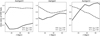 |
Fig. 1 Shapes of DM halos in Auriga 23, 5, and 12, measured in the coordinate system where the z-axis is perpendicular to the stellar disc, and X and Y are the long and short axes of the DM halo in the disc plane. The DM halos of Auriga 23 and 5 are oblate, aligned with the stellar disc (pDM > qDM), and vary little with radius. The DM shape of Auriga 12 varies from being oblate and aligned with the stellar disc (pDM ~ 1 and pDM > qDM) in the inner regions to being vertically aligned with the disc (pDM < qDM and qDM ~ 1) at r ≳ 20 kpc. |
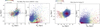 |
Fig. 2 Left: MW observations from LAMOST + Gaia. Right: mock data created for Auriga 23. Each dot represents one star/particle coloured by weight obtained from selection-function correction. There are about 15 000 k giants in the final sample of the smooth halo of the Milky Way. The mock data of Auriga 23 include about 20 000 particles, which generally match the spatial distribution of the MW sample. |
2.3 Mock data
By cross-matching LAMOST with Gaia DR3, we achieve a sample of 619 284k giants; with 3D velocity measured, the typical errors of radial velocity υr and tangential velocities υϕ and υθ are 10, 30, and 30 km/s, respectively. The typical distance error is about 15%. We excluded disc stars chemodynamically to avoid biasing the spatial distribution of the halo. We carefully excluded all substructures, including streams, overdensities, and GES using the friend-of-friend method (Wang et al. 2022; Yang et al. 2019), and we further performed 3σ clipping to remove outliers. In the end, we had 15 000 k giants in the smooth halo with the spatial distribution shown in Fig. 2.
We took three galaxies from the Auriga simulations, Auriga 23, 5, and 12. For each one, we took the following steps to create mock data to mimic LAMOST + Gaia observations for the MW halo.
First, we treated each particle as a single star, transferring their positions and velocities into the ICRS coordinate. We adopted a relative error of 15% for distance, an error of 30 km/s for the tangential velocity in the RA and DEC directions, and an error of 20 km/s for the LOS velocity. The positions and velocities of stars were then perturbed by random numbers, which are normally distributed with dispersions equal to the observational errors.
Second, we performed spatial selection of the stars. We divided the particles into an original bulge with rgc < 4 kpc, an original disc with zgc < 4 kpc, rgc > 4 kpc and Z/Z⊙ > 0.5, and an original halo with the rest. We first randomly selected 1/100 particles from the disc, 1/3 particles from the halo (1/4 for Auriga 12), and no particles from the bulge, and we then performed further spatial selection by only including stars in the northern hemisphere and within a spatial volume similar to the MW LAMOST + Gaia observations, as shown in Fig. 2. This results in ~30 000 stars with the full 6D phase-space information measured. The sample size is much smaller than the original LAMOST + Gaia sample because we took a sparse sampling of the disc stars.
2.4 Data preparation and correction of selection function
With mock data created in an observational manner, we converted the stars into the galactocentric coordinate and obtain the uncertainty of position and velocity in the new coordinate via a bootstrapping process. We cleaned the data and corrected the select function to make it ready for the model construction, in a way similar to how we dealt with the real observations.
First, we used a position-velocity clustering estimator method to identify substructures; we selected the smooth halo by removing all stars identified in substructures with a link length of 0.84 in the 6D distance (Yang et al. 2019). The stellar halos of Auriga 5 and 23 are rather smooth, with no significant structures; we only performed this step on the mock data of Auriga 12. There are fewer substructures in the halo of Auriga simulations than in the real Milky Way galaxy due to the limited mass resolution in the simulation.
Second, we removed the stars from the disc. We integrated the stellar orbits into an initially estimated potential and calculated the circularity, λz, of each orbit. λz is defined as the angular momentum around the z-axis normalised by the maximum allowed by circular orbits with the same binding energy:  , where
  , and
, and  , taking the average of the points along each orbit. A star in a near circular orbit has λz ~ 1, and on a radial orbit it has λz ~ 0. We removed the disc stars in a cut that combines circularity and metallicity; all the stars with λz > 0.8 or λz > 0.5 and Z/Z⊙ > 0.5 were removed. As shown in Fig. 3, the remaining halo stars have an almost symmetric distribution in λz centred at λz = 0.
Third, we cleaned the data by 3σ clipping in the velocity distributions. Although we removed the substructures identified by the clustering estimator method, there are still some particles with high tangential velocities, which are unlikely to be part of a smooth halo in dynamical equilibrium. We also performed a 3σ clipping in υϕ versus υθ to remove the outliers.
Lastly, we corrected for the selection function. For this proof of concept, we used a simple approach by correcting the selection function in the Rgc – zgc plane. We divided the Rgc – zgc plane into 50 × 50 bins in Rgc = [0, 50] kpc and zgc = [0, 50] kpc. We calculated the density of stars in each volume of 2πRgcdRgcdzgc constructed from our sample (ρselect) and that of the original halo before performing spatial selection (ρoriginal). Any star, i, in the bin, j, will have a weight of wi = ρoriginal,j/ρselect,j. Such a selection correction is less accurate at zgc < 4 kpc, where disc stars are mixed in the original halo.
In the end, we were left with about 20 000 stars in the smooth halo; these stars are all located in the northern hemisphere and have the selection function corrected. The final sample of stars with their weights is shown in Fig. 2.
The real selection function of LAMOST is complicated and is corrected by comparing with photometric data, which are considered complete with the magnitude limit (Liu et al. 2017; Yang et al. 2022), resulting in the correction of the selection function in the 3D space, more accurate than what we did here. It is beyond the scope of this paper to test the method of selection function correction. We just wanted the spatial sampling of our mock data to match some major properties of the real observations: (1) the data are not complete in different azimuthal angles, and we have fewer data in the direction of the Galactic centre; (2) the observations at larger distances or with small polar angles are less complete; thus, we obtained larger weights for the stars at these positions. As shown in Fig. 2, the particle weight distribution in our mock data set generally matches the trend in the LAMOST + Gaia MW data.
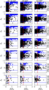 |
Fig. 3 Mock data for Auriga 23. The blue dots are disc stars that we excluded, i.e. stars with λz > 0.8 or stars with λz > 0.5 and Z/Z⊙ > 0.5. The black dots are taken as halo stars and kept in our sample. We divided the data into 7 × 6 bins in rgc versus θ with the intervals of rgc = [5, 8, 12, 16, 22, 30, 40, 50] kpc, θ = [0, 10, 20, 30, 40, 55, 90°]; here, we only show three columns to illustrate the data. |
3 Model construction
We have a sample of stars in the halo, which can be considered complete in the northern hemisphere at rgc ≲ 50 kpc after correction of the selection function. That is, we have the DF of halo stars in 6D phase space f (x, υ) numerically known from the observations. We assumed that the smooth halo is stationary and that the DF of stars integrated in the correct potential matches that directly observed instantaneously. Under this assumption, the DF constructed from the northern hemisphere should be representative of the whole system.
We constructed a dynamical model called the empirical orbit-superposition model according to the following steps: (1) we constructed an adaptable gravitational potential for the MW with a few free parameters; (2) in a gravitational potential with given parameters, we calculated the stellar orbits using stars’ positions and velocities measured as initial conditions and constructed a model by superposing the stellar orbits using the weights of stars given by the selection function correction; (3) we extracted stellar-density distribution and velocity distributions from the orbit-superposition model and evaluated the goodness of the model by calculating the likelihood (χ2) of each model against the data; (4) we explored the parameter grid of the gravitational potential to find the best-fitting models with the maximum likelihood (or least χ2). This method, in principle, is similar to the traditional Schwarzschild orbit-superposition method, but we have the true DF (orbit library and orbit weights) known from the observations. The only assumption we make in this model is that the system is stationary, which is the minimum assumption for all dynamical models. We confirmed the feasibility of this assumption for the smooth halo with a good match between the model and the data, as shown in Section 3.4.
3.1 Gravitational potential
We constructed a model of the gravitational potential by including a bulge, a disc, and a DM halo.
We adopted a Sérsic bulge,
 (2)
(2)
and a MiyamotoNagai disc,
 (3)
(3)
in which  . Our data in the halo do not have strong constraints on the bulge and disc. We fixed the density distribution of the bulge and discs via the true values of the simulation (Grand et al. 2017). We have M*,bulge = 3.2 × 10¹⁰ M⊙, a scale radius of abulge = 1.71 kpc, and a Sérsic index of n = 1.44, M*,disk = 5.6 × 10¹⁰ M⊙. Moreover, we obtain a scale radius of adisk = 4.9 kpc and a scale height of bdisk = 0.25 kpc for Auriga 23. The disc and bulge masses still have some uncertainty for the MW. We tried models with a 20% higher or lower disc mass for Auriga 23 and found no difference in our results. The true values parametrising the bulge and disc of Auriga 5 and Auriga 12 in Grand et al. (2017) are used in our models.
We adopted a flexible, triaxial generalised NFW model for the DM halo, allowing free orientations of the DM halo, and variable 3D shape as a function of radius generally following Vasiliev et al. (2021):
![Mathematical equation: ${\rho _{{\rm{halo}}}} = {\rho _0}{\left( {{{\tilde r} \over {{r_s}}}} \right)^{ - \gamma }}{\left[ {1 + {{\left( {{{\tilde r} \over {{r_s}}}} \right)}^\alpha }} \right]^{{{\gamma - \beta } \over \alpha }}} \times \exp - {\left( {{{\tilde r} \over {{r_{{\rm{cut}}}}}}} \right)^\xi },$](/articles/aa/full_html/2025/11/aa56036-25/aa56036-25-eq8.png) (4)
(4)
in which  , pDM, and qDM are the axis ratios of the DM halo.
The coordinate X ≡ {X, Y, Z} is related to the galactocentric Cartesian coordinate xgc ≡ {xgc, ygc, zgc} by a rotation matrix parametrised by three Euler angles, αq, βq, and γq, as shown in Section 2.3. In principle, all three angles can be left free. Taking into account the degeneracy between the DM orientation and the 3D shape, we fixed βq = 0. The combination of αq and γq determines the DM halo orientation in the XY plane; we fixed γq = 0 and allowed αq to be free in order to test the ability of constraining it. For default models, we also fix αq = 0.
When it is needed, we allowed pDM and qDM to vary as a function of radius with
 (5)
(5)
 (6)
(6)
 (7)
(7)
 (8)
(8)
where  , pin,DM, pout,DM, qin,DM, qout,DM, and the scale radius rq are allowed to be free parameters.
For the radial profile, we fixed α = 1, β = 3 and chose the outer cut-off radius, rcut = 500 kpc, and the cut-off strength, ξ = 5. We started with models for all three mock galaxies with fixed DM orientation (αq = 0, βq = 0 and γq = 0) and constant pDM and qDM. The five parameters in the DM halo, that is, the scale density ρ0 (or the mass Mhalo), the scale radius rs, the inner density slope γ, pDM and qDM, were left as free parameters. For Auriga 12, we further constructed a model with different orientation angles, αq, and a model that allows p(r) and q(r) to vary as a function of radius.
3.2 Orbit integration
Orbit integration was performed using the publicly released AGAMA package (Vasiliev 2019)1. We have about 20 000 stars in the cleaned sample of the smooth halo, with their positions and velocities measured from observations, and the weight of each star obtained from the correction of selection. We started with the position and velocity of the stars from observations and integrated ten orbital periods for each star. We withdrew 1000 particles from each orbit with equal time steps, and each particle was given the weight as the star that initialises the orbit. We superposed particles drawn from the orbits together, thus obtaining an orbit-superposed model, which numerically represents the DF of the stellar system.
3.3 Comparing model and data
The DF of the orbit-superposed model, fmodel(x, υ|potential), is based on data but incorporates the gravitational potential. If the system is in dynamical equilibrium, the DF of the model with the accurate gravitational potential should be statistically the same as that of the stars that initialised it ƒdata(x, υ). We detail particular components of the DF: the spatial density distribution and velocity distributions at different positions. We evaluated the goodness of the model by comparing these with the data.
We calculated the stellar-density distribution in the Rgc–zgc plane, by dividing it into 25 × 25 bins within 50 kpc. The density in each bin is calculated by N/(2πRdRdz) in units of N/kpc3. We calculated the density directly for both the observed data ρdata and the model ρmodel. The uncertainty of the data dρdata is assessed by bootstrapping the position of stars with their uncertainties. The density distributions of the data and model are shown in Fig. 4; we calculated  by directly comparing the data and model:
 (9)
(9)
To analyse velocity distributions, we categorised model particles into bins Nbin = 7 × 6 in r and θ. The divisions are r = [5, 8, 12, 16, 22, 30, 40, 50] kpc and θ = [0, 10, 20, 30, 40, 55, 90°]. We then constructed the velocity distributions (υr, υϕ, υθ) within each bin, as illustrated in Fig. 3. For each velocity component within bin j, we represent its distribution by a histogram using intervals M, labelled as ( ), where k corresponds to the velocities υr, υϕ, and υθ.
In bin j, we have Nj stars, and for a star i with a velocity and measurement uncertainty ( ) within that bin, we determine its likelihood in comparison to the model for each of the three velocity components as follows:
![Mathematical equation: $P_{i,j}^k = {1 \over {\sqrt {2\pi } \times \sigma _i^k}} \times {{\Sigma _{m = 1}^M\,h_{m,j}^k \times \exp \left[ { - {{\left( {\upsilon _i^k - \upsilon _{m,j}^k} \right)}^2}/\left( {2{{\left( {\sigma _i^k} \right)}^2}} \right)} \right]} \over {\Sigma _{m = 1}^M\left( {h_{m,j}^k} \right)}}.$](/articles/aa/full_html/2025/11/aa56036-25/aa56036-25-eq19.png) (10)
(10)
The collective likelihood of all Nj stars in this bin is given by  , and the overall likelihood across all the bins is represented by
  . Due to a deficit of stars at r < 4 kpc, which contributes to the DF of the inner bins, the DF for the innermost bins of our model remains incomplete. Therefore, we omit the first six bins within the r = [5, 8] range in our likelihood calculations. The likelihood across the three velocity components is merged to derive the constraints from the velocity distributions:
 (11)
(11)
Finally, we combine the χ2 values from both the density distribution and velocity distributions to obtain
 (12)
(12)
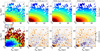 |
Fig. 4 Comparison of stellar-density distribution from data and model for Auriga 23. The top panels from left to right are composed of observational data and several models with different DM axis ratios of qDM and pDM. The colours represent the number density as indicated by the colour bar. and the dashed curves are iso-density contours. The second row shows the uncertainty of the data, and model residuals. The data are well matched by the model with DM qDM = 0.64 and pDM = 1, which are well consistent with the ground truth. The stellar-density distribution constructed by models are either too round or too flat if the shape of underlying DM changes. The stellar-density distribution strongly constrains the 3D shape of the underlying DM halo. |
3.4 Best-fitting models
We investigated the parameter space of ρ0, rs, γ, pDM, and qDM within the gravitational potential. A parameter grid is established with intervals of 0.1, 5 kpc, 0.02, 0.04, and 0.04 for ρ0, rs, γ, pDM, and qDM, respectively. An iterative approach is used to find the optimal models. The process begins with an initial model, and, after developing initial models, iterative refinement follows. During each iteration, we identify the optimal models using the criterion  , where
  . We then generate new models by walking two steps in every direction of the parameter grid of each optimal model. This approach guides the search towards the lower χ2 within the parameter grid and halts when the model with the minimum χ2 is identified. The relatively high value of
  is selected to ensure that all models within a 1σ confidence level are considered before the end of the iteration. Ultimately, we determine the best-fitting models by achieving the minimum
  .
.
We illustrate how the model works using Auriga 23 as an example. In Fig. 4, it is shown that the best-fitting model accurately reproduces the stellar density across the Rgc – zgc plane. Furthermore, it imposes strict constraints on the 3D shape of the underlying DM halo. The shape of the DM halo directly affects the direction of stellar acceleration and thus the shape of the stellar orbits. Variations in the DM halo shape can cause the constructed stellar halo to appear overly flat or excessively round. As shown in Fig. 5, the best-fitting model also reproduces the velocity distributions well in all three components: υr, υϕ, and υθ. These velocity distributions provide strong constraints on the radial density distribution of the DM halo which directly affects the strength of the acceleration, especially in the radial direction. The different radial profiles of the DM halo lead to notable discrepancies in the velocities between the observational data and the model, particularly in υr. Of course, both the stellar-density and velocity distributions are determined by the overall 3D DM distribution, which will be better constrained by combining both.
Our best-fitting model generally reproduces both the density and velocity distributions at various locations in the Rgc – zgc plane, thus validating our assumption of an overall stationary system with the agreement between the model and the data.
However, these stellar systems are never in perfect equilibrium. Although we have tried our best to clean the substructures, there will inevitably be some residual substructures or non-equilibrium features left in the data. For example, in Fig. 5, there are some peaks/bumps in the velocity distributions that are not matched by the model; some of them can indicate residual sub-structures. The υϕ distributions in the bin at 8 < r < 12 kpc close to the disc plane are not perfectly matched by the model either, which can indicate some non-equilibrium features.
In Fig. 6, we illustrate the parameter space explored for Auriga 23. The points denote models within a confidence level of 3σ, coloured according to the normalised  , where
  is the confidence level 1σ determined by bootstrapping2. As shown in Fig. 6, the combination of density distribution and velocity distribution strongly constrains the 3D shape of DM pDM and qDM. Due to the still limited data coverage, there are still strong degeneracies between the three parameters (ρ0, rs, and γ) determining the radial profile.
Nevertheless, the radial density profile within the data coverage is well constrained, as we detail in the next section.
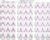 |
Fig. 5 Comparison of velocity distributions from data and model for Auriga 23. The velocity distributions, υr, υϕ, and υθ are calculated in 7 × 6 bins in r versus θ, but we only show three columns here as labelled. In each panel, the grey solid and dashed curves are the velocity distribution and uncertainty of observational data. The red solid curves are from the best-fitting model. Blue and magenta dashed curves show models with different radial distribution of the underlying DM mass. The velocity distributions, especially υr, strongly constrain the underlying DM radial density distribution. The best-fitting model (red solid) reproduces the velocity distributions in all three components well: υr, υϕ, and υθ. |
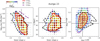 |
Fig. 6 Constraints on parameters of underlying DM distribution for Auriga 23. Each dot represents one model coloured by the relative |


4 Results
We applied the model to mock data created from Auriga 23, Auriga 5, and Auriga 12. In this section, we show our recovery of the DM radial density profile and 3D shape for these three galaxies.
4.1 Recovery of DM density profile
We demonstrate how effectively our models recover the DM radial-density profile and the enclosed DM mass in Fig. 7. Despite significant degeneracy between p0, rs, and γ, our models accurately capture the radial-density profile within the observational range of 4–50 kpc. The uncertainty is larger at r < 8 kpc due to the absence of data.
The enclosed DM mass profile is also well recovered, with a relative uncertainty of about 10%. It should be noted that the DM mass we obtained in the outer regions is 5%–10% higher than the true values but aligns well with the enclosed mass that combines DM and gas. The circumgalactic medium (CGM) in the halo of the simulation mirrors the DM’s density distribution. The mass of the CGM is compensated by an overestimation of the DM mass without a separate gas contribution in our model of the gravitational potential.
4.2 Recovery of the 3D shape of DM
4.2.1 Models with constant qDM and pDM
The three selected galaxies exhibit varied DM halo structures, as illustrated in Fig. 1. The DM halo of Auriga 23 is predominantly oblate, showing minimal change from the inner to the outer regions. The DM halo of Auriga 5 is more triaxial, displaying slight variation. On the other hand, the DM halo of Auriga 12 undergoes notable variations, transitioning from oblate within the inner 20 kpc to a vertical orientation at r > 20 kpc.
Initially, we developed models with constant qDM and pDM for all three galaxies. As depicted in Fig. 8, our model successfully recovered both pDM and qDM for Auriga 23 and Auriga 5, with relatively small uncertainties. For Auriga 12, the model captured the outer configuration of the DM halo, and there is a significant degeneracy between pDM and qDM when the halo is vertically aligned; this is characterised by pDM < qDM.
The stellar-density distribution in the Rgc – zgc plane, especially the flattening of the stellar halo, is crucial to constraining the DM shape. We measure the stellar-halo flattening, qstar, across various radii using isodensity contours and compared these from the data and several models in Fig. 9. The stellar halo of Auriga 23 is notably flat, becoming increasingly so from the centre to the outskirts, and our best-fitting model successfully mimicked qstar at all radii. The stellar halo of Auriga 5 appears rounder, with a tendency to become rounder moving outward; our model approximates the radial variation qstar(r), albeit with moderate inner-region discrepancies. The stellar halo of Auriga 12 is the most spherical, notably rounding from inner to outer areas, with qstar(r) challenging to replicate by a model with a constant DM shape. The failure to reproduce the tendency of qstar(r) suggests a variation of DM shapes from the inner to outer regions.
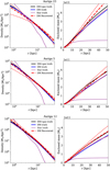 |
Fig. 7 Recovery of DM radial-density distribution. The radial-density profile and enclosed mass profile we obtained for Auriga 23, Auriga 5, and Auriga 12, which are well consistent with the ground truth within 1σ uncertainty, are shown. |
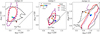 |
Fig. 8 Recovery of DM intrinsic shapes by models with constant qDM and pDM. The panels from left to right are Auriga 23, Auriga 5, and Auriga 12. In each panel, the solid red, black dashed, and purple dashed curves indicate the model 1σ confidence level determined by |


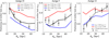 |
Fig. 9 Reproduction of stellar halo flattening qstar as a function of radius Rgc for models with different underlying DM halos. The three panels from left to right are Auriga 23, 5, and 12. The DM halo shapes of Auriga 23 show little variation within our data coverage. The qstar(r) is well reproduced by a model with constant pDM and qDM close to the ground truth. Auriga 5 shows mild variation, and Auriga 12 shows relatively strong variation of the DM halo shape, from r ~ 10 kpc to r ~ 50 kpc. Especially for Auriga 12, the stellar-halo flattening, qstar(r), at all regions can hardly be reproduced by a model with constant pDM and qDM; in contrast, it can be reproduced well by a model with pDM(r) and qDM(r), which vary with radius, close to its ground truth. The stellar-halo flattening qstar(r) has strong constraints on the underlying DM shape. |
4.2.2 Models allowing DM shape to vary from inner to outer regions
We create models with variables pDM(r) and qDM(r) as specified in Eqs. (5)–(8) for Auriga 12. We fixed the transition radius rq = 20 kpc, while the remaining four parameters, qin,DM, qout,DM, pin,DM, and pout,DM were treated as free parameters. The parameters determining the radial DM profile do not degenerate significantly with the 3D shape. To optimise the efficiency of the model, we fixed them at log(ρ0[M⊙/kpc3]) = 6.2, rs = 40 kpc, and γ = 1.6.
The parameter grid we explored for this model is shown in Fig.10. Despite significant uncertainties, a twisted DM halo that is oblate (pin,DM > qin,DM and pin,DM ~ 1) in the inner regions and vertically aligned in the outer regions (pout,DM < qout,DM and qout,DM ~ 1) is strongly favoured.
We derived pDM(r) and qDM(r) from our models within the 1σ confidence level and compared those with the true profiles derived from the simulation. Our model generally recovers the true tendency of the DM shape variation with radius, as shown in the right panels of Fig. 10.
Such models allowing variables pDM(r) and qDM(r) are indeed able to reproduce the stellar-halo-density distribution. We took one of the best-fitting models with pin = 1.04, pout = 0.84, qin = 0.6, and qout = 1.32, which reproduces the surface density distribution well from the inner to outer regions, with the residuals significantly reduced compared to the model with constant pDM and qDM as shown in Fig. 11. The tendency of qstar(r) derived from this model matches the data well (the dashed black curve in Fig. 9).
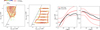 |
Fig. 10 Left: constraints on qin,DM, pin,DM, qout,DM, and pout,DM for model allowing DM axis ratios to vary as a function of radius for Auriga 12. Right: comparison of pDM(r) and qDM(r) profiles obtained by the model (red) and the ground truth (black). The solid and dashed red curves represent the mean and 1σ uncertainty of the results obtained by the model. |
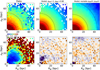 |
Fig. 11 Comparison of stellar-density distribution constructed from data and different models for Auriga 12. The columns from left to right are the data, best-fitting model with constant pDM and qDM, and best-fitting model with pDM(r) and qDM(r) varying as a function of radius, r. The model with constant pDM and qDM cannot match the density distribution in all radial regions; there are significant residuals in the inner 20 kpc. The consistency between data and model improves with the model allowing variable pDM(r) and qDM(r). |
5 Discussion
We fixed the DM orientation with the tilt angle βq = 0. In reality, the DM halo might not be perfectly aligned with the stellar disc. The three galaxies we tested have DM tilt angles of βq ~ 10–15°.
The axis ratio, q, recovered from our model is close to the true axis ratio measured along the fixed zgc axis, not the intrinsic q measured along the principal axes of the DM halo, although the latter two are close to each other when βq is small. For galaxies with a larger tilt angle, βq, we expect the model to still recover q measured along the fixed zgc in a similar way; in this case, it may be significantly different from the intrinsic q measured along the DM principal axes.
The orientation of the DM halo in the xgcygc plane remains largely undetermined. Ideally, if the DM orientation αq can be constrained, we converge two solutions: one with p < 1 and the correct αq and one with p′ = 1/p when αq is misaligned with 90°. In our exploration of the Auriga 12 model that allows a free orientation (αq) of the DM halo in the xgcygc plane, we failed to find significant constraints on αq. In particular, the stellar-density distributions created by various αq values of the DM halo appeared similar, resulting in no constraints on αq from  , and the same is true for the radial velocity distribution υr. The velocities υϕ and υθ are somewhat influenced by the orientation of the DM αq, but this effect occurs in a somewhat unpredictable manner.
This arises because we averaged out information along the azimuthal angle when correcting the selection function and comparing the data with the model. We had to do so because observational data at various azimuthal angles remain incomplete, particularly with a lack of observations directed towards the Galactic centre. Consequently, this process results in a significant level of uncertainty for pDM = Y/X, especially when pDM < qDM, as demonstrated by Auriga 12. Despite this, the relative positioning of pDM and qDM is effectively constrained. In our models for Auriga 12, pDM < qDM is strongly preferred in the outer regions, in contrast to Auriga 23 and 5, where pDM > qDM is strongly preferred.
The stellar halo of the three galaxies we tested is generally in dynamical equilibrium, but inevitably with some residual substructures and non-equilibrium features; they did not introduce obvious systematic bias according to our test results. The LMC, which fell in recently, may have perturbed the Milky Way halo and will affect the results of dynamical modelling. However, the LMC mainly induces a bulk motion in the outskirts of the halo, while it only mildly affects the inner halo, causing a velocity shift in Vz with ~10 km/s at r < 50 kpc (Erkal et al. 2020). Among the Auriga simulations, Auriga 25 had a recent minor merger with mass and orbits similar to the LMC, but its perturbation of the disc and inner halo is significantly stronger than that of the LMC of the Milky Way. We applied the method to Auriga 25 and showed that even with some obvious non-equilibrium in the data, the DM distribution can still be roughly recovered but with larger statistical uncertainty (see the appendix).
6 Summary
We present an empirical, triaxial orbit-superposition model tailored for the MW halo. In this method, we take the minimum assumption of dynamical models whereby the stellar halo is stationary, meaning that the DF in the 6D phase space, f (x, υ), does not change when the stars orbit in the correct gravitational potential. The feasibility of this assumption can be gauged by the final goodness of the match of the data and the model.
The gravitational potential of the model is a combination of disc, bulge, and DM halo with adaptable parameters. Our approach employs a highly flexible triaxial NFW halo, which allows variations in the DM axis ratios (pDM = Y/X, qDM = Z/X) with radius. Within each specified gravitational potential, we take the 6D phase-space information of stars observed as initial conditions, integrate their orbits in the gravitational potential, and form a model by superposing the orbits together. The orbits are weighted by the weights assigned to the stars when correcting the observation selection function. We evaluated the goodness of the model by comparing the DF of the model with that directly constructed from the data, which is expressed in terms of density distribution and velocity distributions (υr, υϕ, υθ) across the Rgc – zgc plane.
This methodology was validated using mock observational data of the MW halo from LAMOST + Gaia with three Auriga galaxies, halo 23, 5, 12, with different intrinsic shapes of the DM halo. The mock data were created with similar spatial selection and observational errors as in LAMOST + Gaia. We cleaned the data by subtracting the disc, substructures, and so on, in exactly the same way as we dealt with the real observational data.
We created models with constant DM axis ratios from all three mock galaxies and extra models allowing pDM(r), qDM(r) to vary with radius for Auriga 12. We find the following:
The density distribution and velocity distributions of the stellar halo provide consistent constraints on the DM distribution. Specifically, the stellar-density distribution has stronger constraints on the DM shape, while velocity distributions better restrict the DM radial-density profile;
The DM radial-density profile and the enclosed DM mass of the three galaxies within the data coverage are well recovered, with a relative uncertainty of about 10%. We still have relatively large uncertainty in each of the three parameters that determine the radial profile (ρ0, rs, and γ) with limited data coverage;
Auriga 23 and Auriga 5 have oblate-to-triaxial DM halos that vary only mildly with radius. The DM axis ratios (pDM, qDM) are well recovered by the models with constant pDM and qDM, and the best-fitting models reproduce the stellar-halo-density distribution reasonably well;
The DM halo of Auriga 12 is twisted, oblate (pDM > qDM) in the inner 20 kpc, and vertically aligned (pDM < qDM) in the outer regions. Our model with constant pDM and qDM recovers those in the outer regions, and it does not reproduce the stellar-halo-density distribution in the inner regions well. We recover pDM(r), qDM(r) of Auriga 12 as a function of radius generally well with a model that allows them to vary, which also better reproduces the stellar-halo-density distribution from inner to outer regions.
Acknowledgements
We thank David Hogg, Jianhui Lian, Zhaozhou Li for useful discussions. LZ acknowledges the support from the CAS Project for Young Scientists in Basic Research under grant No. YSBR-062 and the National Key R&D Program of China No. 2022YFF0503403. X.X.X. acknowledges the support from the National Key Research and Development Program of China No. 2024YFA1611902, CAS Project for Young Scientists in Basic Research grant No. YSBR-062 and YSBR-092, and the science research grants from the China Manned Space Project with No. CMS-CSST-2025-A11.
Appendix A The recovery of DM distributions for Auriga 25
Auriga 25 has a recent minor merger which significantly perturbed its stellar disk and inner halo. The infall orbit and mass of this merger are similar to those of the LMC in the Milky Way, but its perturbation to the disk and inner halo are significantly stronger than the LMC did to the Milky Way.
We orient Auriga 25 in the way that the LMC-like satellite is located in the southern hemisphere, and we take the particles in the north to create the mock data; the stars in the north look closer to dynamical equilibrium with less asymmetrical structures. The mock data are created in a similar way as for the other three galaxies. As shown in Figure A.1, there are significant substructures in the inner halo. We removed the big tail at the end of the disk, but not the other substructures.
We applied the dynamical model to this galaxy in the same way as we did to the three galaxies we showed in the paper. In Figure A.2, we show the recovery of the DM radial density distribution and the 3D shape of the DM halo. In this case, we have larger statistical errors in the results. However, the true DM distribution is still generally recovered by our model within the 1σ confidence level.
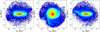 |
Fig. A.1 The surface brightness of Auriga 25 projected with different directions. Its disk was significantly destroyed by a recent merger. Both its stellar disk and its halo are not in fully dynamical equilibrium. |
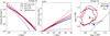 |
Fig. A.2 The recovery of DM radial density distribution and DM 3D shape of Auriga 25, similar to that shown in Figure 7 and Figure 8 for other galaxies. |
References
- Bird, S. A., Xue, X.-X., Liu, C., et al. 2022, MNRAS, 516, 731 [NASA ADS] [CrossRef] [Google Scholar]
- Bovy, J., Bahmanyar, A., Fritz, T. K., & Kallivayalil, N. 2016, ApJ, 833, 31 [NASA ADS] [CrossRef] [Google Scholar]
- Bovy, J., Kawata, D., & Hunt, J. A. S. 2018, MNRAS, 473, 2288 [NASA ADS] [CrossRef] [Google Scholar]
- Bowden, A., Belokurov, V., & Evans, N. W. 2015, MNRAS, 449, 1391 [NASA ADS] [CrossRef] [Google Scholar]
- Erkal, D., Belokurov, V. A., & Parkin, D. L. 2020, MNRAS, 498, 5574 [Google Scholar]
- Grand, R. J. J., Gomez, F. A., Marinacci, F., et al. 2017, MNRAS, 467, 179 [Google Scholar]
- Grand, R. J. J., van de Voort, F., Zjupa, J., et al. 2019, MNRAS, 490, 4786 [Google Scholar]
- Green, G. M., Ting, Y.-S., & Kamdar, H. 2023, ApJ, 942, 26 [Google Scholar]
- Han, J., Wang, W., Cole, S., & Frenk, C. S. 2016, MNRAS, 456, 1017 [Google Scholar]
- Hattori, K., Valluri, M., & Vasiliev, E. 2021, MNRAS, 508, 5468 [NASA ADS] [CrossRef] [Google Scholar]
- Helmi, A. 2004, ApJ, 610, L97 [NASA ADS] [CrossRef] [Google Scholar]
- Ibata, R., Lewis, G. F., Irwin, M., Totten, E., & Quinn, T. 2001, ApJ, 551, 294 [Google Scholar]
- Johnston, K. V., Law, D. R., & Majewski, S. R. 2005, ApJ, 619, 800 [Google Scholar]
- Khoperskov, S., Di Matteo, P., Steinmetz, M., et al. 2025a, A&A, 700, A90 [NASA ADS] [CrossRef] [EDP Sciences] [Google Scholar]
- Khoperskov, S., Steinmetz, M., Haywood, M., et al. 2025b, A&A, 700, A89 [NASA ADS] [CrossRef] [EDP Sciences] [Google Scholar]
- Khoperskov, S., van de Ven, G., Steinmetz, M., et al. 2025c, A&A, 695, A220 [NASA ADS] [CrossRef] [EDP Sciences] [Google Scholar]
- Koposov, S. E., Rix, H.-W., & Hogg, D. W. 2010, ApJ, 712, 260 [Google Scholar]
- Küpper, A. H. W., Balbinot, E., Bonaca, A., et al. 2015, ApJ, 803, 80 [Google Scholar]
- Law, D. R., & Majewski, S. R. 2010, ApJ, 714, 229 [Google Scholar]
- Li, C., & Binney, J. 2022, MNRAS, 510, 4706 [NASA ADS] [CrossRef] [Google Scholar]
- Li, Z., Han, J., Wang, W., et al. 2025, MNRAS, 538, 1442 [Google Scholar]
- Liu, C., Xu, Y., Wan, J.-C., et al. 2017, Res. Astron. Astrophys., 17, 096 [Google Scholar]
- Loebman, S. R., Ivezic, Ž., Quinn, T. R., et al. 2014, ApJ, 794, 151 [NASA ADS] [CrossRef] [Google Scholar]
- Long, R. J., Mao, S., Shen, J., & Wang, Y. 2013, MNRAS, 428, 3478 [Google Scholar]
- Malhan, K., & Ibata, R. A. 2019, MNRAS, 486, 2995 [NASA ADS] [CrossRef] [Google Scholar]
- Nitschai, M. S., Cappellari, M., & Neumayer, N. 2020, MNRAS, 494, 6001 [Google Scholar]
- Pakmor, R., Gómez, F. A., Grand, R. J. J., et al. 2017, MNRAS, 469, 3185 [NASA ADS] [CrossRef] [Google Scholar]
- Palau, C. G., & Miralda-Escudé, J. 2019, MNRAS, 488, 1535 [Google Scholar]
- Palau, C. G., & Miralda-Escudé, J. 2023, MNRAS, 524, 2124 [NASA ADS] [CrossRef] [Google Scholar]
- Portail, M., Gerhard, O., Wegg, C., & Ness, M. 2017, MNRAS, 465, 1621 [NASA ADS] [CrossRef] [Google Scholar]
- Posti, L., & Helmi, A. 2019, A&A, 621, A56 [NASA ADS] [CrossRef] [EDP Sciences] [Google Scholar]
- Prada, J., Forero-Romero, J. E., Grand, R. J. J., Pakmor, R., & Springel, V. 2019, MNRAS, 490, 4877 [NASA ADS] [CrossRef] [Google Scholar]
- Springel, V. 2010, MNRAS, 401, 791 [Google Scholar]
- Tahmasebzadeh, B., Zhu, L., Shen, J., et al. 2024, MNRAS, 534, 861 [NASA ADS] [CrossRef] [Google Scholar]
- Thater, S., Jethwa, P., Tahmasebzadeh, B., et al. 2022, A&A, 667, A51 [NASA ADS] [CrossRef] [EDP Sciences] [Google Scholar]
- van den Bosch, R. C. E., van de Ven, G., Verolme, E. K., Cappellari, M., & de Zeeuw, P. T. 2008, MNRAS, 385, 647 [Google Scholar]
- Vasiliev, E. 2019, MNRAS, 482, 1525 [Google Scholar]
- Vasiliev, E., & Athanassoula, E. 2015, MNRAS, 450, 2842 [Google Scholar]
- Vasiliev, E., Belokurov, V., & Erkal, D. 2021, MNRAS, 501, 2279 [NASA ADS] [CrossRef] [Google Scholar]
- Vera-Ciro, C., & Helmi, A. 2013, ApJ, 773, L4 [Google Scholar]
- Wang, W., Han, J., Cautun, M., Li, Z., & Ishigaki, M. N. 2020, Sci. China Phys. Mech. Astron., 63, 109801 [NASA ADS] [CrossRef] [Google Scholar]
- Wang, F., Zhang, H. W., Xue, X. X., et al. 2022, MNRAS, 513, 1958 [NASA ADS] [CrossRef] [Google Scholar]
- Wegg, C., Gerhard, O., & Bieth, M. 2019, MNRAS, 485, 3296 [NASA ADS] [CrossRef] [Google Scholar]
- Woudenberg, H. C., & Helmi, A. 2024, A&A, 691, A277 [NASA ADS] [CrossRef] [EDP Sciences] [Google Scholar]
- Xue, X. X., Rix, H. W., Zhao, G., et al. 2008, ApJ, 684, 1143 [Google Scholar]
- Yang, C., Xue, X.-X., Li, J., et al. 2019, ApJ, 880, 65 [NASA ADS] [CrossRef] [Google Scholar]
- Yang, C., Zhu, L., Tahmasebzadeh, B., Xue, X.-X., & Liu, C. 2022, AJ, 164, 241 [NASA ADS] [CrossRef] [Google Scholar]
- Zhang, L., Xue, X.-X., Zhu, L., et al. 2025, ApJ, 987, 143 [Google Scholar]
- Zhu, L., van den Bosch, R., van de Ven, G., et al. 2018, MNRAS, 473, 3000 [Google Scholar]
We take the gravitational potential of the best-fitting model and perturb the position and velocity of observed stars with their uncertainty for 100 trials. In each trial, we recompute the model and evaluate the resulting  (including
  and
and  ). The standard deviation of these 100 values χ2 is taken as the confidence level 1σ of the model
  .
.
All Figures
|
Fig. 1 Shapes of DM halos in Auriga 23, 5, and 12, measured in the coordinate system where the z-axis is perpendicular to the stellar disc, and X and Y are the long and short axes of the DM halo in the disc plane. The DM halos of Auriga 23 and 5 are oblate, aligned with the stellar disc (pDM > qDM), and vary little with radius. The DM shape of Auriga 12 varies from being oblate and aligned with the stellar disc (pDM ~ 1 and pDM > qDM) in the inner regions to being vertically aligned with the disc (pDM < qDM and qDM ~ 1) at r ≳ 20 kpc. |
| In the text | |
|
Fig. 2 Left: MW observations from LAMOST + Gaia. Right: mock data created for Auriga 23. Each dot represents one star/particle coloured by weight obtained from selection-function correction. There are about 15 000 k giants in the final sample of the smooth halo of the Milky Way. The mock data of Auriga 23 include about 20 000 particles, which generally match the spatial distribution of the MW sample. |
| In the text | |
|
Fig. 3 Mock data for Auriga 23. The blue dots are disc stars that we excluded, i.e. stars with λz > 0.8 or stars with λz > 0.5 and Z/Z⊙ > 0.5. The black dots are taken as halo stars and kept in our sample. We divided the data into 7 × 6 bins in rgc versus θ with the intervals of rgc = [5, 8, 12, 16, 22, 30, 40, 50] kpc, θ = [0, 10, 20, 30, 40, 55, 90°]; here, we only show three columns to illustrate the data. |
| In the text | |
|
Fig. 4 Comparison of stellar-density distribution from data and model for Auriga 23. The top panels from left to right are composed of observational data and several models with different DM axis ratios of qDM and pDM. The colours represent the number density as indicated by the colour bar. and the dashed curves are iso-density contours. The second row shows the uncertainty of the data, and model residuals. The data are well matched by the model with DM qDM = 0.64 and pDM = 1, which are well consistent with the ground truth. The stellar-density distribution constructed by models are either too round or too flat if the shape of underlying DM changes. The stellar-density distribution strongly constrains the 3D shape of the underlying DM halo. |
| In the text | |
|
Fig. 5 Comparison of velocity distributions from data and model for Auriga 23. The velocity distributions, υr, υϕ, and υθ are calculated in 7 × 6 bins in r versus θ, but we only show three columns here as labelled. In each panel, the grey solid and dashed curves are the velocity distribution and uncertainty of observational data. The red solid curves are from the best-fitting model. Blue and magenta dashed curves show models with different radial distribution of the underlying DM mass. The velocity distributions, especially υr, strongly constrain the underlying DM radial density distribution. The best-fitting model (red solid) reproduces the velocity distributions in all three components well: υr, υϕ, and υθ. |
| In the text | |
|
Fig. 6 Constraints on parameters of underlying DM distribution for Auriga 23. Each dot represents one model coloured by the relative |
| In the text | |
|
Fig. 7 Recovery of DM radial-density distribution. The radial-density profile and enclosed mass profile we obtained for Auriga 23, Auriga 5, and Auriga 12, which are well consistent with the ground truth within 1σ uncertainty, are shown. |
| In the text | |
|
Fig. 8 Recovery of DM intrinsic shapes by models with constant qDM and pDM. The panels from left to right are Auriga 23, Auriga 5, and Auriga 12. In each panel, the solid red, black dashed, and purple dashed curves indicate the model 1σ confidence level determined by |
| In the text | |
|
Fig. 9 Reproduction of stellar halo flattening qstar as a function of radius Rgc for models with different underlying DM halos. The three panels from left to right are Auriga 23, 5, and 12. The DM halo shapes of Auriga 23 show little variation within our data coverage. The qstar(r) is well reproduced by a model with constant pDM and qDM close to the ground truth. Auriga 5 shows mild variation, and Auriga 12 shows relatively strong variation of the DM halo shape, from r ~ 10 kpc to r ~ 50 kpc. Especially for Auriga 12, the stellar-halo flattening, qstar(r), at all regions can hardly be reproduced by a model with constant pDM and qDM; in contrast, it can be reproduced well by a model with pDM(r) and qDM(r), which vary with radius, close to its ground truth. The stellar-halo flattening qstar(r) has strong constraints on the underlying DM shape. |
| In the text | |
|
Fig. 10 Left: constraints on qin,DM, pin,DM, qout,DM, and pout,DM for model allowing DM axis ratios to vary as a function of radius for Auriga 12. Right: comparison of pDM(r) and qDM(r) profiles obtained by the model (red) and the ground truth (black). The solid and dashed red curves represent the mean and 1σ uncertainty of the results obtained by the model. |
| In the text | |
|
Fig. 11 Comparison of stellar-density distribution constructed from data and different models for Auriga 12. The columns from left to right are the data, best-fitting model with constant pDM and qDM, and best-fitting model with pDM(r) and qDM(r) varying as a function of radius, r. The model with constant pDM and qDM cannot match the density distribution in all radial regions; there are significant residuals in the inner 20 kpc. The consistency between data and model improves with the model allowing variable pDM(r) and qDM(r). |
| In the text | |
|
Fig. A.1 The surface brightness of Auriga 25 projected with different directions. Its disk was significantly destroyed by a recent merger. Both its stellar disk and its halo are not in fully dynamical equilibrium. |
| In the text | |
|
Fig. A.2 The recovery of DM radial density distribution and DM 3D shape of Auriga 25, similar to that shown in Figure 7 and Figure 8 for other galaxies. |
| In the text | |
Current usage metrics show cumulative count of Article Views (full-text article views including HTML views, PDF and ePub downloads, according to the available data) and Abstracts Views on Vision4Press platform.
Data correspond to usage on the plateform after 2015. The current usage metrics is available 48-96 hours after online publication and is updated daily on week days.
Initial download of the metrics may take a while.