| Issue |
A&A
Volume 703, November 2025
|
|
|---|---|---|
| Article Number | A160 | |
| Number of page(s) | 18 | |
| Section | Interstellar and circumstellar matter | |
| DOI | https://doi.org/10.1051/0004-6361/202556088 | |
| Published online | 13 November 2025 | |
Large-field CO (1–0) observations towards the Galactic historical supernova remnants: Shocked molecular clouds towards the Crab Nebula
1
Purple Mountain Observatory & Key Laboratory of Radio Astronomy, Chinese Academy of Sciences,
10 Yuanhua Road,
210023
Nanjing,
PR
China
2
School of Astronomy and Space Science, University of Science and Technology of China, Hefei,
Anhui
230026,
PR
China
★ Corresponding author: This email address is being protected from spambots. You need JavaScript enabled to view it.
Received:
24
June
2025
Accepted:
28
August
2025
Abstract
Context. The investigation of the interstellar gas surrounding supernova remnants (SNRs) is not only necessary to improve our knowledge of SNRs, but also to understand the nature of the progenitor systems.
Aims. As part of the Milky Way Imaging Scroll Painting (MWISP) CO line survey, we studied the interstellar gas towards the Galactic historical SNRs. In this work, we present the CO observational results of the Crab Nebula.
Methods. We performed large-field and high-sensitivity CO (1–0) molecular line observations towards the Crab Nebula using the 3×3 beam Superconducting Spectroscopic Array Receiver (SSAR) at the PMO 13.7 m millimeter telescope. The Gaia optical data were used to measure the distances of molecular clouds detected in this work, while the HI data from the GALFA-HI and the HI4PI surveys were used to compare the distributions of the molecular and atomic gas.
Results. The CO observations show molecular clouds towards the Crab Nebula with velocities ranging from about 0 to 16 km s−1. From the CO spectra, we find shocked signatures in the clouds with velocities of roughly [5, 11] km s−1. These shocked molecular clouds, with an angular distance of ~0⋅∘4−0⋅∘5 towards the Crab Nebula, are located at the shell of a bubble discovered in the HI images in the same velocity range. The dimension of the bubble is roughly 2⋅∘3 × 2⋅∘6, and the expansion velocity is ~5 km s−1. The kinetic energy released by the supernova is estimated to be about 3.5 × 1051 erg.
Conclusions. The kinetic energy inferred from the shocked molecular clouds, together with the HI bubble, supports the picture that the Crab Nebula belongs to a typical core-collapse SNR. Nevertheless, due to the significant uncertainty in the distance measurement, further observations are needed to verify the physical association between the shocked molecular clouds and the Crab Nebula.
Key words: ISM: clouds / ISM: kinematics and dynamics / ISM: supernova remnants / ISM: individual objects: Crab Nebula (SN 1054, G184.6-5.8)
© The Authors 2025
 Open Access article, published by EDP Sciences, under the terms of the Creative Commons Attribution License (https://creativecommons.org/licenses/by/4.0), which permits unrestricted use, distribution, and reproduction in any medium, provided the original work is properly cited.
This article is published in open access under the Subscribe to Open model. This email address is being protected from spambots. You need JavaScript enabled to view it. to support open access publication.
1 Introduction
The Crab Nebula, the remnant of the historical supernova of 1054 AD, is one of our prime laboratories in which to study astrophysics and high-energy physics in the Universe (see the review by Hester 2008). This widely studied supernova remnant (SNR) is a synchrotron nebula powered by the Crab Pulsar, enclosed by a bright expanding shell of thermal gas (see reviews by Bühler & Blandford 2014 and Amato & Olmi 2021). The observed dimension of the Crab Nebula is approximately 7′ × 5′, with a position angle of ~126° (measured east of north; e.g. Ng & Romani 2004).
Numerous studies have noted that the kinetic energy of the observed nebula (~3 × 1049 ergs) is far less than the canonical 1051 ergs seen in normal core-collapse supernovae (see Hester 2008 and references therein). It has been suggested that either the Crab Nebula resulted from an unusual low-energy explosion (e.g. Frail et al. 1995; Yang & Chevalier 2015) or there is a large, but as yet undetected, freely expanding shell around the Crab Nebula, which contained most of the kinetic energy of the supernova explosion (e.g. Chevalier 1977). Whether or not a large shell surrounding the nebula is the key to understanding the nature of the Crab Nebula, as well as many branches of astrophysics. Nevertheless, despite long searches at various wavelengths (e.g. Murdin & Clark 1981; Frail et al. 1995; Fesen et al. 1997; Wallace et al. 1999; Sollerman et al. 2000; Seward et al. 2006a), this putative large shell remains unseen.
We started a programme to perform large-field CO observations towards the known Galactic historical SNRs (see e.g. Chen et al. 2017) to study the interstellar gas surrounding them. This programme is part of the Milky Way Imaging Scroll Painting (MWISP1), an unbiased CO(1–0) multi-line survey towards the northern Galactic plane conducted with the Purple Mountain Observatory (PMO) 13.7 m telescope (Su et al. 2019; Sun et al. 2021). In this work we present MWISP CO (1–0) observations towards the Crab Nebula. We note that the Crab Nebula was in the MWISP CO study towards a large catalogue of Galactic SNRs (see Zhou et al. 2023). Nevertheless, the larger-field and, in particular, higher-sensitivity CO data in this work help us to derive new results. In Section 2 we describe the observations and data reduction. Observational results are presented and discussed in Section 3 and summarized in Section 4.
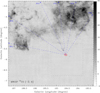 |
Fig. 1 Intensity image of the MWISP 12CO (1–0) emission, integrated in the velocity range −2 to 6 km s−1. The dashed grey square shows the area of deep mapping observations. The red ellipse shows the position and size (7′ × 5′) of the Crab Nebula. The dashed blue arrow lines show the routings of the PV diagrams in Figure 2. |
2 Observations and data reduction
The CO (1–0) observations towards the Crab Nebula were made from September 2016 to November 2020 with the PMO 13.7 m telescope in Delingha, China. A 4° × 4° area, covering ![Mathematical equation: $\[183^{\circ}_\cdot25 \leq l \leq 187^{\circ}_\cdot25\]$](/articles/aa/full_html/2025/11/aa56088-25/aa56088-25-eq3.png) and
and ![Mathematical equation: $\[-7^{\circ}_\cdot25 \leq b \leq -3^{\circ}_\cdot25\]$](/articles/aa/full_html/2025/11/aa56088-25/aa56088-25-eq4.png) , was observed around the Crab Nebula. The nine-beam Superconducting Spectroscopic Array Receiver (SSAR; Shan et al. 2012) was used as the front end in sideband separation mode. Three CO (1–0) lines were simultaneously observed, 12CO in the upper sideband (USB) and two other lines, 13CO and C18O, in the lower sideband (LSB). Typical system temperatures were around 210 K for the USB and around 130 K for the LSB, and the variations among different beams were less than 15%. A fast Fourier transform spectrometer with a total bandwidth of 1 GHz and 16 384 channels was used as the back end. The corresponding velocity resolutions were ~0.16 km s−1 for the 12CO line and ~0.17 km s−1 for both the 13CO and C18O lines.
, was observed around the Crab Nebula. The nine-beam Superconducting Spectroscopic Array Receiver (SSAR; Shan et al. 2012) was used as the front end in sideband separation mode. Three CO (1–0) lines were simultaneously observed, 12CO in the upper sideband (USB) and two other lines, 13CO and C18O, in the lower sideband (LSB). Typical system temperatures were around 210 K for the USB and around 130 K for the LSB, and the variations among different beams were less than 15%. A fast Fourier transform spectrometer with a total bandwidth of 1 GHz and 16 384 channels was used as the back end. The corresponding velocity resolutions were ~0.16 km s−1 for the 12CO line and ~0.17 km s−1 for both the 13CO and C18O lines.
The observations were performed in on-the-fly mode. The total of pointing and tracking errors was about 5″, while the half-power beam width was ~52″ in the 12CO line and ~54″ in the 13CO and C18O lines. The main-beam efficiencies during the observations were ~44% for the USB, with the differences between the beams less than 16%, and ~48% for the LSB, with differences less than 6%.
In the MWISP survey (see Su et al. 2019 and Sun et al. 2021), the typical rms noises were set to ~0.5 K for 12CO (at a velocity resolution of ~0.16 km s−1) and ~0.3 K for 13CO and C18O (at a velocity resolution of ~0.17 km s−1). We deeply mapped a ![Mathematical equation: $\[1^{\circ}_\cdot5 \times 1^{\circ}_\cdot5\]$](/articles/aa/full_html/2025/11/aa56088-25/aa56088-25-eq5.png) area (
area (![Mathematical equation: $\[183^{\circ}_\cdot75 \leq l \leq 187^{\circ}_\cdot25, -6^{\circ}_\cdot75 \leq b \leq -5^{\circ}_\cdot25\]$](/articles/aa/full_html/2025/11/aa56088-25/aa56088-25-eq6.png) ) around the Crab Nebula to obtain much higher sensitivity. The resulting rms noises in this deep area were about 0.25 ± 0.03 K for the 12CO line and about 0.15 ± 0.02 K for the 13CO and C18O lines. Figure A.1 shows the distribution of the 12CO line rms noises in the observations.
) around the Crab Nebula to obtain much higher sensitivity. The resulting rms noises in this deep area were about 0.25 ± 0.03 K for the 12CO line and about 0.15 ± 0.02 K for the 13CO and C18O lines. Figure A.1 shows the distribution of the 12CO line rms noises in the observations.
After removing bad channels and abnormal spectra, and correcting the first-order (linear) baseline fitting, the observed CO data were re-gridded into standard flexible image transport system (FITS) files with a pixel size of 30″ × 30″ (approximately half of the beam size). All data were reduced using the GILDAS package2 and self-developed pipelines.
3 Results and discussion
3.1 Large-field CO mapping area
Figure A.2 shows the large-field (4° × 4°) 12CO velocity channel maps towards the Crab Nebula. A large-scale molecular cloud, in the velocity range from roughly −2 to 6 km s−1, is observed towards the north of the Crab Nebula3. Figure 1 shows the 12CO velocity-integrated intensity image. This large-scale molecular cloud was detected in a previous MWISP CO study towards the Crab Nebula (see Figure 19 in Zhou et al. 2023). Zhou et al. (2023) suggest that the cloud might be associated with the Crab Nebula, though no evidence was found of interaction between them.
It is important to investigate the relationship between the Crab Nebula and the large-scale molecular cloud. Figure 2 shows the position-velocity (PV) diagrams of the Crab Nebula across the cloud (see the PV routings in Fig. 1). No expanding signature is found in any of the various PV directions (see Fig. 2). We further measured the distance to the cloud using a similar method to that described in Yan et al. (2021), based on MWISP CO and Gaia Data Release 3 (DR3) data (Gaia Collaboration 2023). This method uses the principle that molecular clouds usually impose higher optical extinction than other phases of the interstellar medium (ISM). Aided by Bayesian analyses, we derived the distance by identifying the breakpoint in the stellar extinction towards molecular cloud (on-cloud regions) and using the extinction of Gaia stars around the molecular cloud (off-cloud regions) to confirm the breakpoint. The systematic error in the measurement is approximately 5%. The measured distance to the large-scale cloud is roughly 1374 pc (see Figure B.1).
The early estimated distances to the Crab Nebula range from roughly 1400 to 2700 pc (see Trimble 1968, 1973), and an unweighted average of the various methods yields a distance of about 1900 pc (see Trimble 1973). In previous studies of the Crab Nebula, a distance of 2 kpc was generally adopted (see e.g. Hester 2008). Based on more recent very long baseline interferometry observations and Gaia DR3 data, the distance to the Crab Nebula is more precisely estimated to be ![Mathematical equation: $\[1.90_{-0.18}^{+0.22}\]$](/articles/aa/full_html/2025/11/aa56088-25/aa56088-25-eq7.png) kpc (Lin et al. 2023), which is greater than the distance to the north cloud. Based on the PV diagrams and distances measured in the CO observations, we consider there to be no association between the Crab Nebula and the north large-scale molecular cloud. A detailed study of the large-scale cloud is beyond the scope of this work and will be presented in other works in the near future.
kpc (Lin et al. 2023), which is greater than the distance to the north cloud. Based on the PV diagrams and distances measured in the CO observations, we consider there to be no association between the Crab Nebula and the north large-scale molecular cloud. A detailed study of the large-scale cloud is beyond the scope of this work and will be presented in other works in the near future.
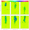 |
Fig. 2 PV diagrams from the Crab across the north molecular cloud (see the routings shown in Figure 1). In each panel, the contours start at 3 σ and then increase in steps of 4 σ, where 1 σ in the large-field 12CO observations is roughly 0.25 K. The red rectangle in the bottom-right corner of each panel shows the angular (52″) and velocity (0.16 km s−1) resolution in the MWISP 12CO observations. |
3.2 Deep CO mapping area
Figure A.3 shows the 12CO velocity channel maps towards the Crab Nebula in the deep observations (see Sect. 2). In the broad bandwidth covering by the MWISP CO survey (16,384 channels, or ±1300 km s−1), the 12CO emission is only detected within a velocity range between 0 and +16 km s−1 towards the Crab region. This is because the Crab Nebula is in the Galactic anticentre direction and the velocities of different arms are coupled together (see e.g. Dame et al. 2001). As seen in Figure A.3, small-scale molecular clouds are found ‘around’ the remnant. According to the velocity continuity of the CO emission, as well as the similarity of the cloud morphology, the CO emission is divided into five velocity ranges: [0, 3], [3, 5], [5, 11], [11, 13], and [13, 16] km s−1. Figures 3a and 3b show the CO intensity images integrated for the individual velocity ranges.
Generally, for a molecular cloud affected by stellar feedback (e.g. stellar wind and/or a supernova shock), its observed CO spectra should show broadened line widths and/or asymmetric (non-Gaussian) line profiles (see e.g. Jiang et al. 2010; Kilpatrick et al. 2016). As seen in Figure A.4, the CO spectra for the molecular clouds detected in the velocity ranges [0, 3], [3, 5], [11, 13], and [13, 16] km s−1 show typical Gaussian line profiles with narrow full width at half maximum (FWHM) line widths (~1–2 km s−1). This suggests that these clouds are quiescent. Therefore, we consider that these molecular clouds are not associated with the Crab Nebula.
On the other hand, the CO spectra of a few molecular clouds in the velocity range [5, 11] km s−1 show line broadening and asymmetry (see CO spectra 6–9 in Figure 4 and the grid spectra in Appendix C). The measured velocity ranges above the baseline (Δv) of the clouds extend to 5–6 km s−1, while the FWHM line width ranges from 2 to 4 km s−1. The observed spectra suggest that these clouds are shocked. We note that no 13CO or C18O line emission from these clouds is detected.
We also tried to measure the distances to the clouds in the velocity range [5, 11] km s−1 using the same method described above. Nevertheless, due to the small angular sizes of the clouds, the number of ‘on-cloud’ stars taken into account is small. Furthermore, the estimated column density of the clouds ranges from ~5 to ~10 × 1021 cm−2 (a CO-to-H2 conversion factor of X = 1.8 × 1020 cm−2 K−1 km−1 s was adopted in the estimation; see Dame et al. 2001), which means that the optical extinction caused by the clouds is also relatively low. Therefore, a large uncertainty remains in the measurements. As seen in Figure B.2, the distance to these clouds is estimated to be ![Mathematical equation: $\[1796_{-121}^{+146}\]$](/articles/aa/full_html/2025/11/aa56088-25/aa56088-25-eq8.png) pc. This distance is comparable to the recently measured distance to the Crab Nebula (
pc. This distance is comparable to the recently measured distance to the Crab Nebula (![Mathematical equation: $\[1.90_{-0.18}^{+0.22}\]$](/articles/aa/full_html/2025/11/aa56088-25/aa56088-25-eq9.png) kpc; Lin et al. 2023).
kpc; Lin et al. 2023).
3.3 Molecular clouds shocked by the Crab?
As introduced in Section 1, the search for the outer shell/shock from the supernova explosion of SN 1054 has taken decades (see e.g. Seward et al. 2006a and Hester 2008, and references therein). Previous HI observations towards the Crab Nebula suggested that the remnant is located within a large, low-density bubble (Romani et al. 1990; Wallace et al. 1994, 1999), roughly 90 pc in radius (at a distance of 2 kpc) and in the velocity range ~[−17, −3] km s−1 (see e.g. Romani et al. 1990). This bubble is thought to have formed as a result of energy input from stellar winds and/or previous supernovae. It is also suggested that such a low-density interstellar gas environment could be the reason for no detection of a radio shell towards the Crab (e.g. Frail et al. 1995; Seward et al. 2006a). Dense molecular knots were observed within the Crab Nebula in the high-angular-resolution observations (Loh et al. 2010, 2011; Wootten et al. 2022). These dense knots, associated with the filaments in the nebula, trace the high-velocity expansion of the nebula caused by the supernova explosion and the pulsar jet. The distribution of the radial velocities of these knots is very asymmetric, and the estimated systemic radial velocity is near 0 km s−1 (see Loh et al. 2011).
Based on the deep CO observations in this work, molecular clouds with shocked signatures are observed towards the south-east of the Crab Nebula, with angular distances ranging from ~![Mathematical equation: $\[0^{\circ}_\cdot4\]$](/articles/aa/full_html/2025/11/aa56088-25/aa56088-25-eq11.png) to ~
to ~![Mathematical equation: $\[0^{\circ}_\cdot5\]$](/articles/aa/full_html/2025/11/aa56088-25/aa56088-25-eq12.png) (see Fig. 3b). Although the observed spectral line widths of these clouds (Δv ~ 5–6 km s−1 and FWHM ~ 2–4 km s−1; see Fig. 4) are smaller than the broadened velocity line widths found in a few SNR-molecular cloud interaction cases, for example IC 433 (>25 km s−1; Dickman et al. 1992), the values are comparable with many other observed interaction cases, such as G16.7+0.1 (Δv ~ 1.5–4.4 km s−1; Reynoso & Mangum 2000) and 3C 397 (Δv ~ 4 km s−1 and FWHM ~ 2.5 km s−1; Jiang et al. 2010). Therefore, these clouds could be affected by the shocks from the SN 1054 supernova, which cause the broadened and asymmetric CO spectra seen in the observations.
(see Fig. 3b). Although the observed spectral line widths of these clouds (Δv ~ 5–6 km s−1 and FWHM ~ 2–4 km s−1; see Fig. 4) are smaller than the broadened velocity line widths found in a few SNR-molecular cloud interaction cases, for example IC 433 (>25 km s−1; Dickman et al. 1992), the values are comparable with many other observed interaction cases, such as G16.7+0.1 (Δv ~ 1.5–4.4 km s−1; Reynoso & Mangum 2000) and 3C 397 (Δv ~ 4 km s−1 and FWHM ~ 2.5 km s−1; Jiang et al. 2010). Therefore, these clouds could be affected by the shocks from the SN 1054 supernova, which cause the broadened and asymmetric CO spectra seen in the observations.
If the shocks from the SN 1054 supernova interacted with these molecular clouds, the velocities of the shocks should reach at least 16 000 km s−1, inferred from a radius of ~![Mathematical equation: $\[0^{\circ}_\cdot5\]$](/articles/aa/full_html/2025/11/aa56088-25/aa56088-25-eq13.png) (or ~17 pc at a distance of 1.9 kpc; see Fig. 3b). Such high velocities have been observed in a few young SNRs, such as Cas A (~15 000 km s−1; see e.g. Fesen et al. 2016) and G1.9+0.3 (~13 000–18 000 km s−1; see e.g. Borkowski et al. 2013, 2017). In this case, the kinetic energy released from the supernova explosion (E0) can be estimated from the shock radius (Rshock) using the Sedov-Taylor evolution mode,
(or ~17 pc at a distance of 1.9 kpc; see Fig. 3b). Such high velocities have been observed in a few young SNRs, such as Cas A (~15 000 km s−1; see e.g. Fesen et al. 2016) and G1.9+0.3 (~13 000–18 000 km s−1; see e.g. Borkowski et al. 2013, 2017). In this case, the kinetic energy released from the supernova explosion (E0) can be estimated from the shock radius (Rshock) using the Sedov-Taylor evolution mode,
![Mathematical equation: $\[R_{\text {shock}} \approx 8\left(\frac{t}{2750 ~\mathrm{yr}}\right)^{\frac{2}{5}}\left(\frac{E_0}{10^{51} ~\mathrm{erg}}\right)^{\frac{1}{5}}\left(\frac{n_0}{1 \mathrm{~cm}^{-3}}\right)^{-\frac{1}{5}} \mathrm{pc},\]$](/articles/aa/full_html/2025/11/aa56088-25/aa56088-25-eq14.png) (1)
(1)
where the shock radius (Rshock) is assumed to be 17 pc and the initial gas density (n0) 0.01 cm−3. From the age of SN 1054, the estimated E0 is ~3.5 × 1051 erg.
Based on very high-energy γ-ray observations, recent studies suggest there is a contribution from hadronic emission from the environment of the Crab Nebula by re-accelerated particles (see e.g. Peng et al. 2022; Spencer et al. 2025), which is somewhat consistent with the shocked molecular clouds found in this work. However, it must be noted that the molecular clouds may be affected by other sources in the region. For example, source SAO 77293 (also known as HD 36879), an O7-type massive star, is located in the region (see Fig. 3b). Its distance, estimated from Gaia parallax data, is roughly 1.8 kpc. The shocked molecular clouds could be affected by the stellar wind from this source. Nevertheless, molecular clouds detected towards SAO 77293 show quiescent spectra in CO observations (see spectra 3–5 in Fig. 4). Further observations, such as high transition CO (or 1720 MHz OH lines) observations, are needed to verify the shock effect towards the molecular clouds in the [5, 11] km s−1 velocity range.
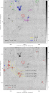 |
Fig. 3 12CO intensity image (grey scale) in the deep observations, integrated within the velocity range [0, 16] km s−1. The red ellipse shows the position and size (7′ × 5′) of the Crab Nebula, while the red dot at the center of the ellipse shows the FWHM beam (52″) in the MWISP 12CO observations at the position of the pulsar ( |
![Mathematical equation: $\[l = 184^{\circ}_\cdot56, ~b = -5^{\circ}_\cdot78\]$](/articles/aa/full_html/2025/11/aa56088-25/aa56088-25-eq10.png)
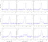 |
Fig. 4 12CO spectra of the clouds in the velocity range [5, 11] km s−1. All the spectra are sampled from a circle with a radius of 90″, and the sampled positions are marked in Figure 3b. |
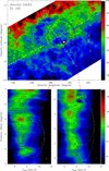 |
Fig. 5 Top: GALFA-HI intensity image, integrated in the velocity range [5, 10] km s−1. The contours correspond to 370, 410, 430, and 450 K km s−1. The red circle shows position of the Crab Nebula. The dashed yellow circles show the bubble and shells distinguished in the HI image, while dashed white arrows show the routings of the PV diagrams shown in the bottom panels. For the two PV diagrams, the contours start from 70 K and then increase in steps of 5 K. The white (partial) ellipses show the fittings towards the cavity-like (spur-like) structures. The white rectangle in the bottom-right corner of the panels shows the angular (4′) and velocity (0.184 km s−1) resolutions in the GALFA-HI survey. |
3.4 A newly discovered HI bubble associated with the shocked clouds
We also checked the HI data from the Galactic Arecibo L-Band Feed Array HI (GALFA-HI; Peek et al. 2018) and HI 4π (HI4PI; HI4PI collaborations et al. 2016) surveys of the Crab Nebula. Figure 5 shows a large-field HI intensity image from the GALFAHI survey. In a velocity range similar to that of the shocked CO clouds, the GALFA-HI image clearly shows a bubble surrounding the Crab Nebula (see also the HI intensity channel maps in Fig. D.1), but the pulsar is far (about 1°) from the centre of the bubble (![Mathematical equation: $\[l = 184^{\circ}_\cdot95, ~b = -4^{\circ}_\cdot95\]$](/articles/aa/full_html/2025/11/aa56088-25/aa56088-25-eq15.png) ). The dimension of the bubble is roughly
). The dimension of the bubble is roughly ![Mathematical equation: $\[2^{\circ}_\cdot3 \times 2^{\circ}_\cdot6\]$](/articles/aa/full_html/2025/11/aa56088-25/aa56088-25-eq16.png) , corresponding to a linear size of about 80 pc × 90 pc (at an assumed distance of 1.9 kpc). Interestingly, concentric shells are also seen outside the bubble, and the diameter of the largest shell is roughly 5° (or 170 pc).
, corresponding to a linear size of about 80 pc × 90 pc (at an assumed distance of 1.9 kpc). Interestingly, concentric shells are also seen outside the bubble, and the diameter of the largest shell is roughly 5° (or 170 pc).
In the HI PV diagrams across the bubble (see Fig. 5), cavity-like structures are detected, which indicates that the bubble is expanding. Furthermore, spur-like protrusions, spatially coincident with the concentric shells seen in the intensity images, are also observed in the PV diagrams (see Fig. 5). The fitted expansion velocities for the bubble and shells are similar to each other (~5 ± 1 km s−1), and the systemic velocity of the bubble and shells is roughly 7.5 km s−1. We also note that (1) relatively low-angular-resolution HI4PI images also show the bubble and the large shell in the same velocity range (images not shown here); and (2) no clear bubble or cavity structures are found in the GALFA-HI images (or HI4PI images) in the velocity range [−20, 0] km s−1 (see Fig. D.2).
Figure 6 compares the distribution of the shocked CO clouds and the HI gas. Here we used the HI4PI HI data instead of the GALFA-HI data due to large-area bad pixels at the position of the Crab Nebula in the GALFA-HI image (see Fig. 5). As seen in Fig. 6, the shocked CO clouds are found at the edge of the HI shell towards the south-east of the Crab Nebula.
The relationship between the Crab Nebula and this newly discovered HI bubble is still uncertain. We did not find extended ionized emission within the bubble in the large-field Hα images (e.g. Finkbeiner 2003). Therefore, the bubble could be opened by stellar wind from massive star(s). Using the method suggested by Weaver et al. (1977), the value of the mechanical luminosity of the wind (Lwind) needed to excavate a bubble with a radius of Rbubble and an expansion velocity of Vexp within a cloud with a density of ngas can be calculated as
![Mathematical equation: $\[L_{\mathrm{wind}} \approx \frac{1}{3}\left(\frac{n_{\mathrm{gas}}}{\mathrm{~cm}^{-3}}\right)\left(\frac{R_{\text {bubble }}}{\mathrm{pc}}\right)^2\left(\frac{V_{\exp }}{\mathrm{km} \mathrm{~s}^{-1}}\right)^3 \times 10^{30} ~\mathrm{erg} \mathrm{~s}^{-1}.\]$](/articles/aa/full_html/2025/11/aa56088-25/aa56088-25-eq18.png) (2)
(2)
With the radius (~45 pc) and expansion velocity (~5 km s−1) measured above, the Lwind is estimated to be ![Mathematical equation: $\[{\sim} 8.4 \times\left(\frac{n_{\text {gas }}}{\mathrm{cm}^{-3}}\right) \times 10^{34} ~\mathrm{erg} ~\mathrm{s}^{-1}\]$](/articles/aa/full_html/2025/11/aa56088-25/aa56088-25-eq19.png) . The kinetic timescale (tkin) of the wind needed to open the bubble was estimated as
. The kinetic timescale (tkin) of the wind needed to open the bubble was estimated as
![Mathematical equation: $\[t_{\text {kin }}(\mathrm{Myr})=\frac{16}{27} \frac{R_{\text {bubble }}}{V_{\text {exp }}},\]$](/articles/aa/full_html/2025/11/aa56088-25/aa56088-25-eq20.png) (3)
(3)
and found to be roughly 5.3 Myr. For the Crab Pulsar, the mass of the progenitor is suggested to be ~8–13 M⊙ (see Hester 2008 and references therein). This kind of massive star is able to drive the stellar wind estimated above, given that the ngas density surrounding the star is less than 1 cm−3. However, the large shell with a diameter of ~5° cannot be opened by the stellar wind from the progenitor of the Crab Pulsar. Other massive stars or supernovae are needed to supply the necessary energy.
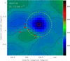 |
Fig. 6 HI4PI HI intensity image, integrated in the velocity range [5, 11] km s−1. The contours start at 320 K km s−1 and then increase in steps of 20 K km s−1. The red contours show the CO emission in the velocity range [5, 11] km s−1 (from Fig 3b), while the dashed yellow circle (radius of |
![Mathematical equation: $\[0^{\circ}_\cdot45\]$](/articles/aa/full_html/2025/11/aa56088-25/aa56088-25-eq17.png)
4 Summary
We present large-field and high-sensitivity CO (1–0) line observations towards the Crab Nebula by the PMO 13.7 m telescope in order to better understand the interstellar gas environment of this well-known historical remnant. The main results of this work are summarized below.
(1) The CO observations show a large-scale molecular cloud, with velocities of −2 to 6 km s−1, to the north of the Crab Nebula. After measuring the distance to the large-scale cloud (~1374 pc), we conclude that the cloud is located in front of the Crab Nebula.
(2) In the deep CO observations, small-scale molecular clouds are detected in the velocity range [0, 16] km s−1 towards the Crab Nebula. The CO spectra indicate that molecular clouds in the velocity range [5, 11] km s−1 have shocked signatures. These clouds, displayed as an arc, are located roughly ![Mathematical equation: $\[0^{\circ}_\cdot4\mathcal{-}0^{\circ}_\cdot5\]$](/articles/aa/full_html/2025/11/aa56088-25/aa56088-25-eq21.png) to the south-east of the Crab Nebula.
to the south-east of the Crab Nebula.
(3) Based on the complementary HI data, we find around the Crab Nebula a large HI bubble, with a dimension of roughly ![Mathematical equation: $\[2^{\circ}_\cdot3 \times 2^{\circ}_\cdot6\]$](/articles/aa/full_html/2025/11/aa56088-25/aa56088-25-eq22.png) and an expansion velocity of ~5 km s−1. The shocked CO clouds are spatially distributed at the edge of the HI shell towards the south-east of the Crab Nebula.
and an expansion velocity of ~5 km s−1. The shocked CO clouds are spatially distributed at the edge of the HI shell towards the south-east of the Crab Nebula.
(4) The combined observational data suggest that the molecular clouds at a velocity of [5, 11] km s−1 are affected by front shocks from the SN 1054 explosion, while the HI bubble could be opened by the stellar wind from its progenitor. In this picture, the kinetic energy released from SN 1054 is estimated to be roughly 3.5 × 1051 erg.
Nevertheless, it must be noted that it is still difficult to confirm an association between the shocked molecular clouds and the Crab Nebula, due to large uncertainty in the distance measurement towards the molecular clouds.
Acknowledgements
We thank the referee for providing insightful suggestions, which helped us to improve this work. This research made use of the data from the Milky Way Imaging Scroll Painting (MWISP) project, which is a multiline survey in 12CO/13CO/C18O along the northern Galactic plane with the PMO 13.7 m telescope. We are grateful to all the members of the MWISP working group, particularly the staff members at the PMO 13.7 m telescope, for their long-term support. MWISP is sponsored by the National Key R&D Program of China with grants 2023YFA1608000, 2017YFA0402701, and the CAS Key Research Program of Frontier Sciences with grant QYZDJ-SSW-SLH047. This work is supported by the National Natural Science Foundation of China (grant No. 12041305). X.C. acknowledges the support from the Tianchi Talent Program of Xinjiang Uygur Autonomous Region.
Appendix A Large-field and deep MWISP CO observations
As we introduced in Section 2, the typical rms noise in the MWISP survey was about 0.5 K for the 12CO line (at a velocity resolution of ~0.16 km s−1). To obtain higher sensitivity, we deeply mapped a ![Mathematical equation: $\[1^{\circ}_\cdot5 \times 1^{\circ}_\cdot5\]$](/articles/aa/full_html/2025/11/aa56088-25/aa56088-25-eq23.png) area (
area (![Mathematical equation: $\[183^{\circ}_\cdot75 \leq l \leq 185^{\circ}_\cdot25, -6^{\circ}_\cdot75 \leq b \leq-5^{\circ}_\cdot25\]$](/articles/aa/full_html/2025/11/aa56088-25/aa56088-25-eq24.png) ) around the Crab Nebula, in which the rms noise was about 0.25 ± 0.03 K for 12CO. Figure A.1 shows the rms distribution in the MWISP observations. Figure A.2 shows the large-field (4° × 4°) 12CO velocity channel maps toward the Crab Nebula. Figure A.3 shows the 12CO velocity channel maps toward the Crab Nebula in the deep (
) around the Crab Nebula, in which the rms noise was about 0.25 ± 0.03 K for 12CO. Figure A.1 shows the rms distribution in the MWISP observations. Figure A.2 shows the large-field (4° × 4°) 12CO velocity channel maps toward the Crab Nebula. Figure A.3 shows the 12CO velocity channel maps toward the Crab Nebula in the deep (![Mathematical equation: $\[1^{\circ}_\cdot5 \times 1^{\circ}_\cdot5\]$](/articles/aa/full_html/2025/11/aa56088-25/aa56088-25-eq25.png) ) observations. Figure A.4 shows the sampled 12CO spectra.
) observations. Figure A.4 shows the sampled 12CO spectra.
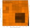 |
Fig. A.1 Distribution of rms noises in the MWISP 12CO (1–0) observations (velocity resolution of ~0.16 km s−1) toward the Crab Nebula. The unit of the scale bar is K. The relatively dark region shows the deep mapping area in the CO observations. The red ellipse shows the position and size (7′ × 5′) of the Crab Nebula, while the red dot at the center of the remnant shows the FWHM beam (52″) in the MWISP 12CO observations at the position of the pulsar ( |
![Mathematical equation: $\[l = 184^{\circ}_\cdot56, ~b = -5^{\circ}_\cdot78\]$](/articles/aa/full_html/2025/11/aa56088-25/aa56088-25-eq26.png)
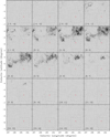 |
Fig. A.2 Velocity-integrated intensity channel maps of the MWISP 12CO (1–0) emission in the large-field observations. The integrated velocity range is written in the bottom-left corner of each panel (in km s−1). The plotting scale for each panel is same (from −2 to 9 K km s−1). In each panel, the dashed grey square shows the area of deep mapping observations, while the red ellipse shows the position and size (7′ × 5′) of the Crab Nebula. |
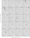 |
Fig. A.3 Velocity-integrated intensity channel maps of the MWISP 12CO (1–0) emission in the deep observations. In each panel, contour levels correspond to 3, 5, 7, 10, 14 σ, then increase in steps of 5 σ, where the 1 σ level is ~0.16 K km s−1. The integrated velocity range is written in the bottom left corner of each panel (in km s−1). The red ellipse shows the position and size (7′ × 5′) of the Crab Nebula, while the red dot at the center of the ellipse shows the FWHM beam (52″) in the MWISP 12CO observations at the position of the pulsar ( |
![Mathematical equation: $\[l = 184^{\circ}_\cdot56, ~b = -5^{\circ}_\cdot78\]$](/articles/aa/full_html/2025/11/aa56088-25/aa56088-25-eq27.png)
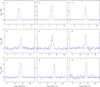 |
Fig. A.4 12CO spectra of the clouds in the velocity ranges of [0, 3] km s−1 (spectra No. 1–3), [3, 5] km s−1 (spectrum No. 4), [11, 13] km s−1 (spectrum No. 5), and [13, 16] km s−1 (spectra No. 6–9). All the spectra are sampled in a circle with a radius of 90″, and the sampled positions are marked in Figure 3a. |
Appendix B The distances of the molecular clouds
Based on the MWISP 12CO and Gaia DR3 data (Gaia Collaboration 2023), we measure the distances toward the molecular clouds in the observed region, using the same method as described in Yan et al. (2021). As seen in Figure B.1, a large-scale molecular cloud is seen to the northeast of the Crab Nebula. The distance measured for this molecular cloud is ~ 1374 pc. Therefore, this cloud is located in front of the Crab Nebula. For the shocked molecular clouds to the southeast of the Crab Nebula (see Figure B.2), larger uncertainty remains in the distance measurement, due to the small angular sizes and column densities of these clouds. The estimated distance of these clouds is roughly 1800 pc.
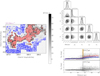 |
Fig. B.1 Measured distance toward the north large-scale cloud. The left panel shows the MWISP 12CO intensity image. The black contour shows the edge of molecular cloud (3 σ threshold), while red and blue dots represent on- and off-cloud Gaia DR 3 stars. In the right bottom panel, red and blue points represent on- and off-cloud stars (binned every 5 pc), respectively. The dashed green line is the modeled extinction AG. The distance is derived with raw on-cloud Gaia DR3 stars, which are represented with gray points. The black vertical lines indicate the distance (D) estimated with Bayesian analyses and Markov Chain Monte Carlo (MCMC) sampling, and the shadow area depicts the 95% highest posterior density (HPD) distance range. The plots of the MCMC samples are displayed in the right top panel (distance, the extinction of foreground and background stars and uncertainties). The mean and 95% HPD of the samples are shown with solid and dashed vertical lines, respectively. |
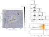 |
Fig. B.2 Same as Figure B.1 but with the clouds in the velocity range [5, 11] km s−1. |
Appendix C The CO spectra of the shocked molecular clouds
Figure C.1 shows the 12CO intensity from Figure 3b, while Figure C.2 shows the grid 12CO spectra superposed on the intensity images.
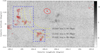 |
Fig. C.1 12CO velocity-integrated intensity image (same as the Fig. 3b). The two blue dashed-line rectangles mark the regions for showing the 12CO grid spectra. |
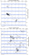 |
Fig. C.2 Grid 12CO spectra of the regions marked in Fig. C.1, superposed on the 12CO intensity images. The temperature and velocity ranges are shown in the bottom-left panel for the two images. The grid spacing is 3′ for the top image and 1.5′ for the bottom image. |
Appendix D The GALFA-HI channel maps and intensity image
Figure D.1 shows the GALFA-HI channel maps in the velocity range from 0 to 12 km s−1, in which detailed information about the distribution and kinematics of the HI gas can be found. Figure D.2 shows the GALFA-HI intensity image integrated within the [-20, 0] km s−1.
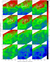 |
Fig. D.1 Velocity-integrated intensity channel maps of the GALFA-HI emission. The integrated velocity range is written in the left top corner of each panel (in km s−1). The unit of the scale bar is K km s−1. For all panels, red circle marks the position of the Crab Nebula. The overlapped white contour (1.5 K km s−1) shows the MWISP 12CO intensity image integrated within the same velocity range as the HI emission. |
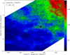 |
Fig. D.2 GALFA-HI intensity image integrated in the velocity range of [-20, 0] km s−1. The unit of the scale bar is K km s−1. The contours start from 200 K km s−1, and then increase by steps of 100 K km s−1. The red circle shows the position of the Crab Nebula. |
References
- Amato, E., & Olmi, B. 2021, Universe, 7, 448 [NASA ADS] [CrossRef] [Google Scholar]
- Borkowski, K. J., Reynolds, S. P., Hwang, U., et al. 2013, ApJ, 771, L9 [NASA ADS] [CrossRef] [Google Scholar]
- Borkowski, K. J., Gwynne, P., Reynolds, S. P., et al. 2017, ApJ, 837, L7 [NASA ADS] [CrossRef] [Google Scholar]
- Bühler, R., & Blandford, R. 2014, Rep. Prog. Phys., 77, 066901 [NASA ADS] [CrossRef] [Google Scholar]
- Chen, X., Xiong, F., & Yang, J. 2017, A&A, 604, A13 [NASA ADS] [CrossRef] [EDP Sciences] [Google Scholar]
- Chevalier, R. A. 1977, Supernovae, 66, 53 [Google Scholar]
- Dame, T. M., Hartmann, D., & Thaddeus, P. 2001, ApJ, 547, 792 [Google Scholar]
- Dickman, R. L., Snell, R. L., Ziurys, L. M., et al. 1992, ApJ, 400, 203 [Google Scholar]
- Fesen, R. A., & Milisavljevic, D. 2016, ApJ, 818, 17 [Google Scholar]
- Fesen, R. A., Shull, J. M., & Hurford, A. P. 1997, AJ, 113, 354 [Google Scholar]
- Finkbeiner, D. P. 2003, ApJS, 146, 2, 407 [Google Scholar]
- Frail, D. A., Kassim, N. E., Cornwell, T. J., et al. 1995, ApJ, 454, L129 [Google Scholar]
- Gaia Collaboration (Vallenari, A., et al.) 2023, A&A, 674, A1 [NASA ADS] [CrossRef] [EDP Sciences] [Google Scholar]
- Hester, J. J. 2008, ARA&A, 46, 127 [Google Scholar]
- HI4PI Collaboration (Ben Bekhti, N., et al.) 2016, A&A, 594, A116 [NASA ADS] [CrossRef] [EDP Sciences] [Google Scholar]
- Jiang, B., Chen, Y., Wang, J., et al. 2010, ApJ, 712, 1147 [NASA ADS] [CrossRef] [Google Scholar]
- Kilpatrick, C. D., Bieging, J. H., & Rieke, G. H. 2016, ApJ, 816, 1 [Google Scholar]
- Lin, R., van Kerkwijk, M. H., Kirsten, F., et al. 2023, ApJ, 952, 161 [Google Scholar]
- Loh, E. D., Baldwin, J. A., & Ferland, G. J. 2010, ApJ, 716, L9 [Google Scholar]
- Loh, E. D., Baldwin, J. A., Curtis, Z. K., et al. 2011, ApJS, 194, 2, 30 [Google Scholar]
- Murdin, P., & Clark, D. H. 1981, Nature, 294, 543 [Google Scholar]
- Ng, C.-Y., & Romani, R. W. 2004, ApJ, 601, 479 [Google Scholar]
- Peek, J. E. G., Babler, B. L., Zheng, Y., et al. 2018, ApJS, 234, 2 [Google Scholar]
- Peng, Q.-Y., Bao, B.-W., Lu, F.-W., et al. 2022, ApJ, 926, 7 [NASA ADS] [CrossRef] [Google Scholar]
- Reynoso, E. M., & Mangum, J. G. 2000, ApJ, 545, 874 [NASA ADS] [CrossRef] [Google Scholar]
- Romani, R. W., Reach, W. T., Koo, B. C., et al. 1990, ApJ, 349, L51 [Google Scholar]
- Seward, F. D., Gorenstein, P., & Smith, R. K. 2006a, ApJ, 636, 873 [NASA ADS] [CrossRef] [Google Scholar]
- Seward, F. D., Tucker, W. H., & Fesen, R. A. 2006b, ApJ, 652, 1277 [NASA ADS] [CrossRef] [Google Scholar]
- Shan, W., Yang, J., Shi, S., et al. 2012, IEEE Trans. Terahertz Sci. Technol., 2, 593 [Google Scholar]
- Sollerman, J., Lundqvist, P., Lindler, D., et al. 2000, ApJ, 537, 861 [Google Scholar]
- Spencer, S. T., Mitchell, A. M. W., & Reville, B. 2025, A&A, 698, A131 [NASA ADS] [CrossRef] [EDP Sciences] [Google Scholar]
- Su, Y., Yang, J., Zhang, S., et al. 2019, ApJS, 240, 9 [Google Scholar]
- Sun, Y., Yang, J., Yan, Q.-Z., et al. 2021, ApJS, 256, 32 [NASA ADS] [CrossRef] [Google Scholar]
- Trimble, V. 1968, AJ, 73, 535 [Google Scholar]
- Trimble, V. 1973, PASP, 85, 579 [NASA ADS] [CrossRef] [Google Scholar]
- Wallace, B. J., Landecker, T. L., & Taylor, A. R. 1994, A&A, 286, 565 [NASA ADS] [Google Scholar]
- Wallace, B. J., Landecker, T. L., Kalberla, P. M. W., et al. 1999, ApJS, 124, 181 [Google Scholar]
- Weaver, R., McCray, R., Castor, J., et al. 1977, ApJ, 218, 377 [NASA ADS] [CrossRef] [Google Scholar]
- Wootten, A., Bentley, R. O., Baldwin, J., et al. 2022, ApJ, 925, 1, 59 [Google Scholar]
- Yan, Q.-Z., Yang, J., Su, Y., et al. 2021, ApJ, 922, 8 [NASA ADS] [CrossRef] [Google Scholar]
- Yang, H., & Chevalier, R. A. 2015, ApJ, 806, 153 [NASA ADS] [CrossRef] [Google Scholar]
- Zhou, X., Su, Y., Yang, J., et al. 2023, ApJS, 268, 61 [NASA ADS] [CrossRef] [Google Scholar]
All the directions mentioned in this work are in the Galactic coordinate system.
All Figures
|
Fig. 1 Intensity image of the MWISP 12CO (1–0) emission, integrated in the velocity range −2 to 6 km s−1. The dashed grey square shows the area of deep mapping observations. The red ellipse shows the position and size (7′ × 5′) of the Crab Nebula. The dashed blue arrow lines show the routings of the PV diagrams in Figure 2. |
| In the text | |
|
Fig. 2 PV diagrams from the Crab across the north molecular cloud (see the routings shown in Figure 1). In each panel, the contours start at 3 σ and then increase in steps of 4 σ, where 1 σ in the large-field 12CO observations is roughly 0.25 K. The red rectangle in the bottom-right corner of each panel shows the angular (52″) and velocity (0.16 km s−1) resolution in the MWISP 12CO observations. |
| In the text | |
|
Fig. 3 12CO intensity image (grey scale) in the deep observations, integrated within the velocity range [0, 16] km s−1. The red ellipse shows the position and size (7′ × 5′) of the Crab Nebula, while the red dot at the center of the ellipse shows the FWHM beam (52″) in the MWISP 12CO observations at the position of the pulsar ( |
| In the text | |
|
Fig. 4 12CO spectra of the clouds in the velocity range [5, 11] km s−1. All the spectra are sampled from a circle with a radius of 90″, and the sampled positions are marked in Figure 3b. |
| In the text | |
|
Fig. 5 Top: GALFA-HI intensity image, integrated in the velocity range [5, 10] km s−1. The contours correspond to 370, 410, 430, and 450 K km s−1. The red circle shows position of the Crab Nebula. The dashed yellow circles show the bubble and shells distinguished in the HI image, while dashed white arrows show the routings of the PV diagrams shown in the bottom panels. For the two PV diagrams, the contours start from 70 K and then increase in steps of 5 K. The white (partial) ellipses show the fittings towards the cavity-like (spur-like) structures. The white rectangle in the bottom-right corner of the panels shows the angular (4′) and velocity (0.184 km s−1) resolutions in the GALFA-HI survey. |
| In the text | |
|
Fig. 6 HI4PI HI intensity image, integrated in the velocity range [5, 11] km s−1. The contours start at 320 K km s−1 and then increase in steps of 20 K km s−1. The red contours show the CO emission in the velocity range [5, 11] km s−1 (from Fig 3b), while the dashed yellow circle (radius of |
| In the text | |
|
Fig. A.1 Distribution of rms noises in the MWISP 12CO (1–0) observations (velocity resolution of ~0.16 km s−1) toward the Crab Nebula. The unit of the scale bar is K. The relatively dark region shows the deep mapping area in the CO observations. The red ellipse shows the position and size (7′ × 5′) of the Crab Nebula, while the red dot at the center of the remnant shows the FWHM beam (52″) in the MWISP 12CO observations at the position of the pulsar ( |
| In the text | |
|
Fig. A.2 Velocity-integrated intensity channel maps of the MWISP 12CO (1–0) emission in the large-field observations. The integrated velocity range is written in the bottom-left corner of each panel (in km s−1). The plotting scale for each panel is same (from −2 to 9 K km s−1). In each panel, the dashed grey square shows the area of deep mapping observations, while the red ellipse shows the position and size (7′ × 5′) of the Crab Nebula. |
| In the text | |
|
Fig. A.3 Velocity-integrated intensity channel maps of the MWISP 12CO (1–0) emission in the deep observations. In each panel, contour levels correspond to 3, 5, 7, 10, 14 σ, then increase in steps of 5 σ, where the 1 σ level is ~0.16 K km s−1. The integrated velocity range is written in the bottom left corner of each panel (in km s−1). The red ellipse shows the position and size (7′ × 5′) of the Crab Nebula, while the red dot at the center of the ellipse shows the FWHM beam (52″) in the MWISP 12CO observations at the position of the pulsar ( |
| In the text | |
|
Fig. A.4 12CO spectra of the clouds in the velocity ranges of [0, 3] km s−1 (spectra No. 1–3), [3, 5] km s−1 (spectrum No. 4), [11, 13] km s−1 (spectrum No. 5), and [13, 16] km s−1 (spectra No. 6–9). All the spectra are sampled in a circle with a radius of 90″, and the sampled positions are marked in Figure 3a. |
| In the text | |
|
Fig. B.1 Measured distance toward the north large-scale cloud. The left panel shows the MWISP 12CO intensity image. The black contour shows the edge of molecular cloud (3 σ threshold), while red and blue dots represent on- and off-cloud Gaia DR 3 stars. In the right bottom panel, red and blue points represent on- and off-cloud stars (binned every 5 pc), respectively. The dashed green line is the modeled extinction AG. The distance is derived with raw on-cloud Gaia DR3 stars, which are represented with gray points. The black vertical lines indicate the distance (D) estimated with Bayesian analyses and Markov Chain Monte Carlo (MCMC) sampling, and the shadow area depicts the 95% highest posterior density (HPD) distance range. The plots of the MCMC samples are displayed in the right top panel (distance, the extinction of foreground and background stars and uncertainties). The mean and 95% HPD of the samples are shown with solid and dashed vertical lines, respectively. |
| In the text | |
|
Fig. B.2 Same as Figure B.1 but with the clouds in the velocity range [5, 11] km s−1. |
| In the text | |
|
Fig. C.1 12CO velocity-integrated intensity image (same as the Fig. 3b). The two blue dashed-line rectangles mark the regions for showing the 12CO grid spectra. |
| In the text | |
|
Fig. C.2 Grid 12CO spectra of the regions marked in Fig. C.1, superposed on the 12CO intensity images. The temperature and velocity ranges are shown in the bottom-left panel for the two images. The grid spacing is 3′ for the top image and 1.5′ for the bottom image. |
| In the text | |
|
Fig. D.1 Velocity-integrated intensity channel maps of the GALFA-HI emission. The integrated velocity range is written in the left top corner of each panel (in km s−1). The unit of the scale bar is K km s−1. For all panels, red circle marks the position of the Crab Nebula. The overlapped white contour (1.5 K km s−1) shows the MWISP 12CO intensity image integrated within the same velocity range as the HI emission. |
| In the text | |
|
Fig. D.2 GALFA-HI intensity image integrated in the velocity range of [-20, 0] km s−1. The unit of the scale bar is K km s−1. The contours start from 200 K km s−1, and then increase by steps of 100 K km s−1. The red circle shows the position of the Crab Nebula. |
| In the text | |
Current usage metrics show cumulative count of Article Views (full-text article views including HTML views, PDF and ePub downloads, according to the available data) and Abstracts Views on Vision4Press platform.
Data correspond to usage on the plateform after 2015. The current usage metrics is available 48-96 hours after online publication and is updated daily on week days.
Initial download of the metrics may take a while.