| Issue |
A&A
Volume 703, November 2025
|
|
|---|---|---|
| Article Number | A298 | |
| Number of page(s) | 13 | |
| Section | Numerical methods and codes | |
| DOI | https://doi.org/10.1051/0004-6361/202556221 | |
| Published online | 27 November 2025 | |
Modeling solar atmosphere dynamics with MAGEC
1
Instituto de Astrofísica de Canarias,
38205
La Laguna,
Tenerife,
Spain
2
Dpto. de Astrofísica, Universidad de La Laguna,
38205
La Laguna,
Tenerife,
Spain
★ Corresponding author: This email address is being protected from spambots. You need JavaScript enabled to view it.
Received:
2
July
2025
Accepted:
22
October
2025
Abstract
Context. Modeling the solar atmosphere is challenging due to its layered structure and dynamic multi-scale processes.
Aims. We aim to validate the new radiative magnetohydrodynamic (MHD) code MAGEC—built by integrating the MANCHA3D and MAGNUS codes into a finite-volume, shock-capturing framework—and to explore its capabilities through 2D simulations of magnetoconvection in the solar atmosphere.
Methods. The MAGEC code is parallelized with Message Passing Interface (MPI), enabling efficient scalability for large-scale simulations. We have enhanced it with advanced numerical techniques to address the specific complexities of the solar corona, including a module for local thermodynamic equilibrium (LTE) radiative coronal losses. To address the small time steps due to large heat flux values, we adopted the hyperbolic treatment for the thermal conduction of MANCHA3D, which significantly improves the computational times. In addition, we estimated the effective numerical resistivity and viscosity through a dedicated set of experiments. To evaluate the robustness and accuracy of MAGEC, we performed a series of 2D simulations covering a domain extending from 2 Mm below the solar surface to 18.16 Mm into the corona. Simulations were conducted with both open and closed magnetic field configurations. For each case, we analyzed the resulting steady-state temperature profiles and examined the energy contributions at different heights. In addition, we investigated the influence of the perpendicular component of thermal conduction in a dedicated simulation.
Results. The MAGEC code effectively reproduced expected temperature profiles based on the boundary conditions applied and the imposed magnetic field configuration. All simulations reached a thermally stable state. When using an open vertical magnetic field, the temperature in the middle corona was higher than in the case with a closed, arcade-like magnetic field structure. We quantified the contributions to the internal energy from all explicit and implicit terms in the steady state, both in terms of temporal averages and as functions of height, as well as their relative contributions to total heating and cooling. In a second phase of the study, we investigated the role of the perpendicular component of thermal conduction, which is often neglected in coronal models, and found that it can influence plasma dynamics around reconnection events. Although local effects are modest, their cumulative impact can lead to measurable changes in the average temperature profile.
Conclusions. Through detailed validation, MAGEC is a reliable and efficient code for radiative MHD simulations of the solar atmosphere. The integration of shock-capturing methods is particularly well suited to modeling the plasma environment, effectively handling the shocks and discontinuities characteristic of the solar atmosphere. MAGEC is a robust tool for high-fidelity magneto-convection simulations of the solar atmospheric dynamics.
Key words: conduction / convection / magnetohydrodynamics (MHD) / methods: numerical / Sun: atmosphere / Sun: corona
© The Authors 2025
 Open Access article, published by EDP Sciences, under the terms of the Creative Commons Attribution License (https://creativecommons.org/licenses/by/4.0), which permits unrestricted use, distribution, and reproduction in any medium, provided the original work is properly cited.
This article is published in open access under the Subscribe to Open model. This email address is being protected from spambots. You need JavaScript enabled to view it. to support open access publication.
1 Introduction
Modeling the solar atmosphere presents a significant computational challenge because of the complexity and diversity of its structure. The solar atmosphere comprises multiple layers -each with distinct dynamics, physical processes, and scales - that interact intricately with each other. From the convective motions in the photosphere to the highly structured magnetic fields in the corona, each layer requires specific modeling techniques to accurately capture its unique characteristics. Developing a code that can address these diverse and dynamic processes is a complex task. As our understanding of solar physics deepens and computational capabilities advance, it becomes crucial to continuously improve and adapt numerical codes to better capture the complexities inherent in the solar atmosphere.
The simulation of the solar atmosphere has evolved considerably over the past few decades, with successive studies incorporating increasingly sophisticated physics and numerical methods. Several representative works have focused on the layers up to the photosphere. For example, Stein & Nordlund (1998) investigated solar granulation using the STAGGER code, emphasizing convective motions and energy transport in the absence of magnetic fields. Steiner et al. (1998) explored the interaction between magnetic flux sheets and granular convection, highlighting dynamic phenomena such as shock formation, using an early version of the CO5BOLD code. Vögler et al. (2005) developed the MURAM code to simulate solar magneto-convection, analyzing the concentration and amplification of magnetic flux. Stein & Nordlund (2006) used STAGGER to study small-scale magneto-convection and the evolution of magnetic flux. Furthermore, Jacoutot et al. (2008), using the SOLARBOX code, examined the influence of magnetic fields on convection and acoustic oscillations.
Further studies have extended into the chromosphere, where additional complexities arise from this layer’s partial ionization and strong interactions with radiation. Schaffenberger et al. (2005) introduced the CO5BOLD code to model the solar atmosphere from the convection zone to the chromosphere, focusing on dynamic magnetic flux reshuffling, shock propagation, and flux tube formation. Using an earlier version of the BIFROST code (Gudiksen et al. 2011), Carlsson et al. (2010) performed 3D radiative MHD simulations to investigate chromospheric heating, emphasizing mechanisms such as Ohmic dissipation, magnetic field interactions, and swirling motions as channels for energy transport. More recently, Khomenko et al. (2018) employed the MANCHA3D code (Modestov et al. 2024) to study the role of ambipolar diffusion in wave propagation, Poynting flux absorption, and chromospheric heating, highlighting the importance of ion-neutral interactions in the partially ionized chromospheric plasma.
Increasing the complexity of solar models, several studies have succeeded in including the solar corona within the same computational domain as the convection zone and chromosphere. Among the first to achieve this were Abbett (2007), using the RADMHD code, and Hansteen et al. (2007), who employed 3D MHD simulations with the STAGGER code to model the dynamic coupling between these layers. These pioneering works highlighted the role of magneto-convection in driving energy and magnetic flux transport and emphasized the importance of magnetic connectivity in shaping coronal structures and enabling energy dissipation for heating.
Later, Rempel (2017) extended the MURaM code to simulate the corona, incorporating key physical processes such as optically thin radiative losses, field-aligned thermal conduction, and the Boris correction to manage high Alfvén speeds. Similarly, the BIFROST code (Gudiksen et al. 2011) - which includes non-gray, non-LTE radiative transfer, field-aligned thermal conduction, ambipolar diffusion, and the Hall effect - was employed by Martínez-Sykora et al. (2017, 2020) to investigate the influence of ion-neutral interactions and non-equilibrium ionization on chromospheric heating and spicule dynamics.
The two-fluid JOANA code (Wójcik et al. 2018) has been widely used for many solar applications. For example, Murawski et al. (2022) demonstrated how granulation-generated waves and plasma viscosity can balance radiative losses in the chromosphere. The MAGNUS code, derived from earlier work by Navarro et al. (2017) and built on the CAFE (Lora-Clavijo et al. 2015) and Newtonian-CAFE (González-Avilés et al. 2015) codes, has been applied to model chromospheric jets (Navarro et al. 2021) and flux emergence (Navarro et al. 2019).
The RAMENS code was used by Iijima et al. (2023) to simulate the formation of the solar wind, highlighting the roles of convection-driven wave excitation and magnetic reconnection. The R2D2 code was used by Toriumi et al. (2024) to study the impact of magnetic flux tube twist on flux emergence, revealing key processes underlying active region formation. A wide range of applications in solar and astrophysical plasma modeling have also been carried out using codes such as AMRVAC (Keppens et al. 2023), LARE3D (Arber et al. 2001), PENCIL (Pencil Code Collaboration 2021), PLUTO (Mignone et al. 2007), and GOEMHD3 (Skála et al. 2015).
Expanding into stellar contexts, Chiavassa et al. (2024) reviewed simulations performed with CO5BOLD (Freytag 2013, 2017) and Athena++ (Stone et al. 2008), uncovering the globalscale nature of convection in cool, evolved stars and its significant role in driving stellar winds and mass loss. Similarly, Canivete Cuissa & Teyssier (2022) used the RAMSES code to investigate stellar magneto-convection. Incorporating adaptive mesh refinement techniques for large-scale solar simulations, the codes DISPATCH (Popovas 2025) and DYABLO (Delorme et al. 2025) are being developed.
These codes adopt a variety of numerical methods. Some use finite-volume methods with shock-capturing schemes such as CO5BOLD, RAMSES, MAGNUS, JOANA, DISPATCH, and DYABLO. The rest employ finite-difference methods, and some have modular frameworks such as AMRVAC and PLUTO that support both schemes. Among the codes that implement shockcapturing schemes, only CO5BOLD, JOANA, DISPATCH, and DYABLO have been used to simulate magneto-convection. Of these, only JOANA has employed a simulation domain that extends into the corona and includes key coronal physics, such as radiative losses and thermal conduction.
Finite-volume methods with high-resolution shock-capturing techniques are particularly well suited to simulations of the solar atmosphere, as they are designed to handle complex fluid dynamics. Unlike traditional numerical schemes, advanced approaches such as Godunov-type methods use approximate Riemann solvers to accurately capture shocks and discontinuities (Toro 2009). These techniques allow the resolution of sharp gradients and abrupt changes in the plasma state without relying on artificial diffusivity, which can obscure the underlying physics. However, their implementation is generally more complex than finite-difference schemes, and they may require more computational resources, especially in multi-dimensional setups.
In this paper, we present the new numerical code MAGEC, which takes advantage of shock-resolving finite volume techniques. The paper is organized as follows: Section 2 provides a detailed introduction to the newly developed MAGEC code. The fundamental equations governing the simulations are outlined in Section 2.1, followed by a description of the numerical schemes implemented in Section 2.2. The thermal conduction model and its implementation are discussed in Section 2.3, while the equation of state is presented in Section 2.4. Section 2.5 gives an overview of the radiative modules, and Section 2.6 describes the calculation of the numerical resistivity and viscosity. The simulation setup and results are presented in Section 3. Finally, Section 4 provides a summary of the main findings and a discussion of potential future research.
2 Description of the MAGEC code
The MAGEC code is a finite volume-based tool developed to model MHD phenomena in the solar atmosphere and other astrophysical environments. It employs shock-capturing methods for high-precision simulations. MAGEC integrates the MANCHA3D code (Modestov et al. 2024) with the MAGNUS code (Navarro et al. 2017), merging the advanced numerical schemes of MAGNUS with the efficient, MPI-parallelized framework of MANCHA3D and its physical modules.
Beyond incorporating MAGNUS’s core schemes, MAGEC includes critical modules from MANCHA3D for optically thick LTE radiative transfer, thermal conduction, and non-ideal physics derived from plasma partial ionization in the single-fluid approximation (ambipolar diffusion and Hall effects), though the latter features are not applied in the present study. The code also integrates a newly developed module for coronal thin radiative losses. This section offers a comprehensive overview of each component within the code.
2.1 Equations
A gravitationally stratified plasma under the influence of thermal conduction and radiative terms can be represented by the following set of equations:
 (1)
(1)
 (2)
(2)
![Mathematical equation: & \frac{\partial (\rho {\bf v})}{\partial t} + \nabla \cdot \left[ \rho {\bf v} {\bf v} + \left( p + \frac{{\bf B}^2}{2\mu_0} \right) {\bf I} - \frac{{\bf B B} }{\mu_0} \right] = \rho {\bf g} , \label{eq:rhoV} \\](/articles/aa/full_html/2025/11/aa56221-25/aa56221-25-eq3.png) (3)
(3)
![Mathematical equation: & \frac{\partial e}{\partial t} + \nabla \cdot \left[ \left( e + p + \frac{{\bf B}^2}{2 \mu_0} \right){\bf v} - \frac{\bf B}{\mu_0} \left( {\bf B \cdot v} \right) \right] \label{eq:energy} \\ & \hspace{3.5 cm} = \rho {\bf v} \cdot {\bf g} - \nabla \cdot {\bf q} + \qradEQ + \qlossEQ , \nonumber](/articles/aa/full_html/2025/11/aa56221-25/aa56221-25-eq4.png) (4)
(4)
where ρ is the density, v is the velocity, p is the gas pressure, B is the magnetic field, g is the gravitational acceleration, q is the heat flux vector, Qrad/Qloss are the radiative terms in optically thick/thin plasma, and μ0 is the magnetic permeability of free space. The dot “•” represents the scalar product of vectors, while the notation “BB” stands for the tensor product and I is the identity tensor. In Equation (4), e represents the total energy per unit volume given by
 (5)
(5)
where eint is the internal energy per unit volume given by the equation of state, which is discussed in Section 2.4.
2.2 Numerical methods
The same system of Equations (1)–(4) can be written in the conservative form
 (6)
(6)
where U is the vector of conservative variables, F is the flux dyad and S is the vector of source/sink terms given by U = [ρ,ρv, e, B]T,
 (7)
(7)
and
 (8)
(8)
The equations are solved using the method of lines, which transforms PDEs into ODEs via spatial discretization with a finite volume (FV) approach, followed by time integration,
 (9)
(9)
where  ,
,  , and
, and  are the numerical fluxes at the interfaces of a cell and are calculated using highresolution shock capturing methods (HRSC), which couple slope limiters and Riemann solvers.
The modular structure of the code allows for a flexible combination of numerical methods. For time integration, the code includes third-order Strong-Stability preserving Runge-Kutta time-steppers (SSP-RK3) (Gottlieb et al. 2001) as well as fourth-and sixth-order standard Runge-Kutta schemes. The available HRSC methods include the Riemann solvers HLL (Harten et al. 1983), HLLC (Li 2005), and HLLD (Miyoshi & Kusano 2005) and the slope limiters: MINMOD (Roe 1986), MC (Van Leer 1977), Van Leer (van Leer 1974), Ospre (Waterson & Deconinck 2007), and WENO5 (Titarev & Toro 2004). The code uses the Flux Constrained Transport method (Evans & Hawley 1988) to prevent the divergence of magnetic field from growing in time due to numerical errors.
The time step due to advection is
 (10)
(10)
where Ccfl stands for the Courant number, and  is the speed of the fastest wave present traveling in direction d = x, y, z at the grid cell indexed by (i, j, k). The minimum is taken over all grid cells of the domain. The values of
  are obtained from the eigenvalues of the Jacobian matrix associated with the system of Equation (6). For instance, in the x-direction, they are given by
 (11)
(11)
where vα is the Alfvén speed and cf and cs are the fast and slow magnetosonic speeds given by
 (12)
(12)
with a the speed of sound.
2.3 Thermal conductivity
The effects of thermal conduction (TC) are represented by the term ∇ • q in the energy Equation (4). In the strongly magnetized regime, the heat flux is aligned with the magnetic field,
 (13)
(13)
where ∇|| gives the projection in the parallel direction to the magnetic field and κ|| is the thermal conductivity. This approximation is valid for most astrophysical applications and is commonly referred to as Spitzer’s (Spitzer 1956) thermal conduction.
If the magnetization is not strong, the propagation of heat along the other directions can be expressed in the following form
 (14)
(14)
where ∇⊥ = ∇ - ∇|| is the projection operator in the perpendicular direction to the magnetic field, and the last term is the projection in the transverse direction (second perpendicular direction to the magnetic field). Braginskii (1965) deduced the general expressions for the conductivity coefficients (κ||, κ⊥ and κ×) for electrons and ions in terms of the plasma properties like density, temperature, pressure and magnetic field. In the case of electrons, they are given by
 (15)
(15)
 (16)
(16)
 (17)
(17)
and for ions,
 (18)
(18)
 (19)
(19)
 (20)
(20)
Here the subscripts and superscripts e and i denote the electrons and ions, respectively. The pressures and masses of the two species are represented by pe, pi, me, and mi. The collision frequencies are given as νii for ion-ion collisions and νei for electron-ion collisions. The variables xi and xe represent the ratio of the cyclotron frequency (Ω) to the collision frequency (ν) for each species, respectively,
 (21)
(21)
where
 (22)
(22)
 (23)
(23)
e is the electron charge, Zi is the charge of the ion, ne and ni are the electron and ion number densities. All definitions are in SI units. The Coulomb logarithm can be approximated by:
 (24)
(24)
for Te < 50 eV, with ne given in cm−3 and Te in electronvolts. From these expressions, we can see that in the case of a null magnetic field, the heat flux becomes isotropic q = −κ||∇T since xe = 0 and  .
.
The parallel conductivity values predicted by the two models are nearly identical, with the value in the Spitzer model being 1.013094636 times that predicted by the Braginskii model. The difference between the models lies in their treatment of conduction: the Spitzer model considers only conduction along the magnetic field, whereas the Braginskii model accounts for propagation in all directions.
The numerical treatment of thermal conduction is challenging in regions with high temperatures and strong magnetic fields. Under these conditions, the parallel component of the heat flux becomes too high, causing a reduction of the timestep associated with heat conduction. To overcome this difficulty, we use the hyperbolic heat-conduction equation, which allows for larger timesteps.
This equation modifies the classical Fourier heat flux by adding a thermal inertia term. It was independently proposed by Vernotte (1958) and Cattaneo (1958) to resolve the paradox of infinite propagation speed in Fourier’s theory, leading to the concept of thermal waves. This approach has been extensively studied both theoretically and experimentally (see Abdel-Hamid 1999 and references therein). In astrophysics, it was first applied to model field-aligned diffusion of cosmic rays by Snodin et al. (2006) and later introduced in solar simulations by Rempel (2017) in the MURAM code. It has since been implemented in the PENCIL code (Warnecke & Bingert 2020), the MANCHA code (Navarro et al. 2022), and the BIFROST code (Cherry et al. 2024).
This method introduces an additional hyperbolic equation to evolve the parallel component of the heat flux q||. The equation is given by
 (25)
(25)
Here f sat is the saturation factor used for stability,
 (26)
(26)
and τ is the relaxation time, which should be calibrated depending on the problem. For the simulations used in this paper we used a value of τ = 10Δt.
In the code, the user can select the thermal conduction model appropriate for their simulation: either the Braginskii or Spitzer formulation for solar plasma conditions, or, for more general MHD applications, specify constant conductivity values manually. Additionally, the user can choose between a hyperbolic or parabolic treatment.
2.4 Equation of state
The system of equations is closed using an equation of state (EOS) for the solar chemical composition, as provided by Anders & Grevesse (1989). The internal energy per unit volume, density, and electron pressure are precomputed over a temperature-pressure grid, following the algorithm of Mihalas (1967), which is based on the Saha equation. This EOS accounts for the effects of both first and second atomic ionization for all elements up to Z = 92, as well as the formation of hydrogen molecules. The EOS results are stored in lookup tables, enabling efficient conversion between thermodynamic quantities. For more details check Vitas & Khomenko (2015) and Modestov et al. (2024).
2.5 Radiative terms
The radiative loss term in the optically thick plasma of the sub-photospheric regions, photosphere, and low chromosphere (Qrad) is calculated by solving the non-gray radiative transfer (RT) equation under the assumption of LTE, using a domain decomposition following Vögler et al. (2005). The wavelength dependence of emission and absorption coefficients is discretized through the opacity binning method (Nordlund 1982). For the simulations discussed in this paper, a single bin was used, corresponding to the gray approximation. Angle integration is performed using quadrature with three rays per octant. The RT module’s formal solver is based on the short-characteristics method by Olson & Kunasz (1987). A detailed description is provided in Modestov et al. (2024).
While the LTE assumption limits the accuracy of the RT module in regions above the photosphere, we turn off this term in regions with temperatures higher than 20000 [K], for which we used an approximation for radiative losses in the optically thin plasma of the form
 (27)
(27)
where the electron/hydrogen number densities ne/nH are given by
 (28)
(28)
with X = 0.7 begin hydrogen abundance, and mp the proton mass. We use the tabulated loss function Λ(T) from the CHIANTI 10.1 database (Dere et al. 2023) with photospheric abundances. Since the loss rate function in the database is provided for a specific particle density, we average the loss function over the range of 108 to 1012 particles per cm3. The resulting loss function is illustrated in Fig. 1.
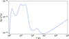 |
Fig. 1 Density-averaged radiative loss rate Λ(T) from the CHIANTI 10.1 database with photospheric abundances. |
2.6 Numerical resistivity and viscosity
To estimate the numerical resistivity and viscosity of the code, we performed a series of experiments in which we introduced additional terms into the source vector to account for both effects. The modified source vector is given by:
 (29)
(29)
where η is the resistivity and Π is the viscous stress tensor given by
 (30)
(30)
with ν representing the kinematic shear viscosity.
To evaluate the numerical resistivity in our experiments, we evolved a series of magneto-convection simulations using an arcade-like magnetic field configuration, varying the explicit resistivity. The specific details of the simulation setup are presented in the following section. Starting from a baseline snapshot in the steady-state regime, we performed multiple simulations with different resistivity values, each evolved for one solar second. At the end of this period, we measured the maximum amplitude of the magnetic field. The top panel of Figure 2 shows the maximum value of the magnetic field amplitude decreasing as the resistivity value grows.
The numerical resistivity is estimated by locating the value of η for which the change in the maximum magnetic field amplitude is above the numerical noise threshold, such as that arising from round-off errors. We determined the numerical noise threshold as follows. For each simulation, we computed the average of the maximum magnetic field amplitude, denoted as  , along with its standard deviation σi. The ratio
  provides an estimate of the numerical variations that arise from round-off errors. We then identified the maximum value of this ratio in all simulations. Finally, we define the numerical noise threshold as the difference between the maximum magnetic field amplitude obtained from the zero-resistivity experiment and the largest numerical variation estimated among the simulations. This is
 (31)
(31)
The top panel of Figure 2 shows that the intersection of the fitting function with the noise threshold (horizontal red dashed line) is when η = ηnum = 1.023 × 10³m2/s. To estimate the numerical viscosity, we followed the same procedure but varied the values of ν and calculated the maximum speed instead of the maximum magnetic field amplitude. In this case, the numerical noise is
 (32)
(32)
where σi corresponds now to the standard deviation of the maximum speed in each simulation. The corresponding plot is presented in the bottom panel of Figure 2. In such a case, we find that the numerical viscosity is νnum = 4.509 × 10³ m2/s.
To estimate the numerical resistivity, we focused on variations in the magnetic field amplitude, since resistivity appears in the induction equation and directly influences the magnetic field. While other physical quantities are also affected, the most significant variations are expected in the magnetic field. Following the same logic, we used the maximum velocity variations to estimate the numerical viscosity. Because viscosity acts as a dissipative term in the momentum equation, it primarily affects the momentum and velocity more rapidly than other variables.
It is important to note that the procedure used to estimate the numerical resistivity and viscosity provides only a simple approximation. The obtained values give an order-of-magnitude estimate, but in theory, they should not be constant. Moreover, the values we obtained may be valid only for our experiments, as they depend on the resolution, the Riemann solver, and the flux limiters employed. To obtain more accurate values, more specialized experiments should be carried out, for instance, as done by Rembiasz et al. (2017).
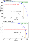 |
Fig. 2 Graphical estimation of numerical resistivity (top panel) and numerical viscosity (bottom panel). Each dot represents the maximum magnetic field (Bmax) or velocity (Vmax) obtained from a simulation with a specific explicit value of η or ν. The blue solid line is a fit to these data points. Two horizontal lines are shown: one corresponds to the Bmax/Vmax value for the case with η = 0 and ν = 0, and the other marks the threshold of numerical noise. The intersection of this threshold with the fitted curve defines the estimated numerical resistivity or viscosity, indicated by the vertical line. |
3 Coronal simulations
3.1 Initial setup
The initial atmospheric structure for the simulations is constructed by combining several solar models. At heights [−2,0] Mm, with z = 0 defined as the height where the continuum optical depth at 500 nm equals 1, we employed the solar convection zone model from Spruit (1974). This setup is connected to the VAL-C model (Vernazza et al. 1981) used in the height range [0, 2] Mm and is smoothly extended to z = 3 Mm where the temperature stabilizes at 1MK from [3, 18.16] Mm. The transition between models is achieved by imposing the hydrostatic equilibrium and ensuring consistency with the EOS. Figure 3 displays the initial density and temperature vertical profiles.
In all simulations, the computational domain spans 46.08 × 20.16 Mm2, extending from 2 Mm below the solar surface to 18.16 Mm above. The simulations use 2304 × 1440 points, providing a resolution of 20 km horizontally and 14 km vertically. Random noise was introduced to the internal energy to initiate the instability.
Horizontal boundary conditions (BC) are periodic, while the bottom boundary is open to allow mass flow, with automated control applied to regulate the fluctuation of the mass and entropy, as done in Khomenko et al. (2018). The upper boundary has symmetric (zero gradient) conditions imposed on the internal energy, density, vx, vy, and Bz and antisymmetric conditions on Bx and By. In all simulations, the temperature at the top boundary is kept to its initial value. For the vertical velocity vz, we used an outflow condition, and it is set to zero when it is negative, thus preventing inflows:
 (33)
(33)
where vz(N) and vz(N-1) are the top boundary points.
We first developed the convection instability in a simulation without a magnetic field, with q= 0 and Qloss= 0. Once convection is fully developed and the system stabilizes, we extract a snapshot at t = 1000 s, which we use as the base state for all subsequent simulations. Figure 5 shows a logarithmic color map of the temperature for this snapshot, overlaid with velocity field arrows, whose lengths are proportional to the local flow speed. At sub-surface depths, the plot reveals well-developed convective granules. However, in the overlying layers, the upward flows generated by the convective motions disrupt the coronal plasma, resulting in disorganized and unstructured mixing. This behavior is a consequence of the absence of a magnetic field, which in reality plays a crucial role in regulating and structuring coronal dynamics. While this scenario does not occur in nature, it serves as an intermediate step in the development of our models.
After 1000s add either of the two different magnetic fields to the base hydrodynamic convective structure: the first one is a 10 G vertical magnetic field, the second one is a potential arcadelike magnetic field given by
 (34)
(34)
 (35)
(35)
where B0 = 10 G, z0 = −2 Mm, k = 2π/Lx and Lx = 46.08 Mm is the horizontal size of the domain (figure 6). The magnetic field is either constant or potential and therefore is initially consistent with the equations because it is force-free. Then, convection smoothly moves the magnetic field to make it consistent with the flow structures.
Figure 4 presents one-dimensional vertical profiles of the plasma-beta for each implanted magnetic field configuration, evaluated at the center of the domain along the x-direction. The horizontal line indicates the location where plasma-beta equals one, marking the transition between pressure-dominated and magnetically dominated regions. Both configurations become magnetically dominated at approximately the same height (z ≈ 1 Mm), though the vertical field case exhibits a lower plasmabeta compared to the arcade configuration. In the arcade case, plasma-beta rises again, indicating a return to pressure domination around z ≈ 12 Mm.
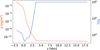 |
Fig. 3 Initial profiles of density and temperature as functions of height. |
3.2 Results
We performed a total of 4 simulations evolved for one hour of solar time, including a simulation featuring the arcade-like magnetic field, with Spitzer’s thermal conduction model. We use the minmod slope-limiter, the HLLC Riemann solver, and the SSP-RK3 time integration method. Table 1 summarizes the main characteristics of each simulation and includes hyperlinks to animations of the density and temperature. The column Field indicates the magnetic field configuration, and the column TC refers to the thermal conduction model applied (either Braginskii, B; or Spitzer, S).
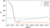 |
Fig. 4 Initial plasma-beta profiles as a function of height, evaluated at the center of the domain in the x-direction, for both the vertical and arcade magnetic field configurations after field implantation. |
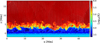 |
Fig. 5 Color map of the temperature from the baseline hydrodynamic simulation at t = 1000 s. Arrows indicate the velocity field, with lengths proportional to the local flow speed. The associated movie is available online. |
 |
Fig. 6 Color map of the magnetic field strength in gauss and field line configuration of the arcade-like model. |
3.2.1 Overview of the simulations
Intermediate states from Simulations 2 and 3 are shown in Figure 7, corresponding to the vertical and arcade-like magnetic field configurations, respectively. The snapshots were taken at 30 minutes of solar time - halfway through the total simulation duration. The full-time evolution for all simulations is available via the links provided in Table 1. The color map represents the logarithm of the temperature, with magnetic field lines overlaid using equally spaced seed points. Velocity vectors are also plotted, with arrow lengths proportional to the local flow speed.
A prominent feature in both cases is the preservation of the overall magnetic field topology above the surface. In Simulation 2, the field retains its predominantly vertical configuration, while in Simulation 3, the arcade-like structure remains largely intact. In both simulations, elongated structures form along the magnetic field lines.
The transition region behaves differently between the two configurations. In the arcade-like field simulation, it appears significantly broader beneath the loop system, where temperatures remain cooler than in areas with a predominantly vertical field.
The velocity field exhibits a clear trend with height: the flow speed generally increases with altitude. However, the flow does not strictly follow the direction of the magnetic field -particularly in the arcade-like configuration, where significant deviations are observed in the upper regions. These deviations occur mainly in areas where the plasma β > 1, as evident from the plasma β profile shown in Fig. 4. In the regions where β < 1, the flow is more closely aligned with the magnetic field; nevertheless, the alignment is not exact, since the plasma β is less than unity but not sufficiently small to enforce a strong coupling. In contrast, in the vertical field case, the inclination of the velocity vectors relative to the magnetic field lines is considerably smaller, indicating a more aligned flow, as expected.
Below z = 0 Mm, in the sub-convection region, both simulations exhibit similar thermal and dynamic behavior. The temperature profiles are comparable, and the granulation pattern - including cell size - is consistent across both runs. However, the magnetic field evolution differs: in the arcade-like field simulation, strong concentrations of magnetic field develop near the footpoints, forming localized, high-intensity braided structures.
For the statistical analysis, we compute the horizontal average of the temperature over the last 20 minutes of each simulation. The left panel of Figure 8 shows the horizontally averaged temperature as a function of height and time. The color map on the left corresponds to the vertical magnetic field case, while the one on the right corresponds to the arcade-like magnetic field case. Contour lines are overlaid to highlight three specific temperature levels: 104.5 K, 105.5 K, and 105.9 K. The first contour, 104.5 K, is characteristic of chromospheric temperatures; the second contour, 105.5 K, also shows little temporal variation and appears to maintain a height around z = 6 Mm in the vertical field case but about 1 Mm higher in the arcade-like configuration. This indicates that, beyond the transition region, the vertical field case maintains a hotter corona than the arcade-like case. The third contour, 105.9 K, shows greater oscillations in the arcade-like case, consistent with Figure 7, which shows that the coronal temperature depends in this case on the magnetic field inclination.
The right panel of Figure 8 presents the temperature averaged both horizontally and over time. The black dotted line indicates the initial temperature profile. The most significant difference between the two cases occurs in the height range z = [5,10] Mm, where the vertical field case retains a much hotter corona. The maximum temperature difference between the two models reaches approximately 135 kK. Comparing the time-averaged profiles to the initial state clearly shows that neither of the two models achieves a restoration of the chromospheric heating. Vertical error bars represent the standard deviation, which quantifies the variations of the horizontally averaged temperature over time. The variations are minimal in the solar interior (z < 0 Mm), peak in the transition region, and decrease again towards the corona. The vertical field case exhibits smaller deviations overall, consistent with both the left panel and the color maps of Figure 7.
To illustrate the overall behavior of the magnetic field divergence, Figure 9 shows the time evolution of the maximum and average values of the dimensionless error associated to the divergence of the magnetic field defined as |∇ ∙ B|∆x/(|B| + 〈|B|〉h). Here, the value of the average of the magnetic field is used to avoid indeterminations. The plot in the top corresponds to all the values in the domain, and the other two correspond to the heights z = 0 and z =10 Mm. The difference between the average and maximum errors spans approximately two orders of magnitude, both across the full domain and at fixed heights. Furthermore, the error is larger in the lower regions of the atmosphere and decreases in the upper layers, consistent with a stronger field in the near-surface convection. The bottom panels display the logarithmic color map of the error for an intermediate snapshot at t=2800s, shown for both simulations. These results demonstrate that, on average, the constrained transport method (Evans & Hawley 1988) is effective in maintaining the solenoidal condition of the magnetic field. However, they also indicate that the method does not completely eliminate local violations of the divergence-free constraint.
Summary of simulation parameters.
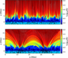 |
Fig. 7 Color map of the logarithmic temperature distribution after 1 hour of solar time. The top panel shows the simulation with a vertical magnetic field (Simulation 2), and the bottom panel shows the simulation with an arcade-like magnetic field (Simulation 3). The arrows indicate the velocity field, with lengths proportional to the local flow speed, bthe blacklines are magnetic field lines. |
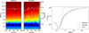 |
Fig. 8 Horizontally averaged temperature profiles for the simulations shown in Fig. 7 for the last 20 minutes. The left panel displays the horizontally averaged temperature as a function of height and time, with contour lines overlaid to highlight specific temperature values. The right panel shows the temperature averaged both horizontally and over time. The black dotted line indicates the initial profile. |
3.2.2 Energy contributions
To study the processes that most strongly influence the thermal structure of the atmosphere in our simulations, we considered the evolution equation for the internal energy:
 (36)
(36)
where ∇ ∙ (eintv) represents the internal energy flux, p∇ ∙ v the pressure work, ∇ ∙ q the thermal conduction contribution, Qloss the optically thin radiative losses, Qrad the optically thick radiative term. We included the numerical resistive heating, ηnum J2, and the numerical viscous dissipation term, ∇ ∙ (Πnum ∙ v), however both of them are implicit terms. We estimated the values of ηnum and νnum back in Section 2.6.
Figure 10 shows the horizontally and temporally averaged contributions to the internal energy equation, computed over the final 20 minutes of each simulation. For clarity, values smaller than 1 × 10⁻¹⁰ are omitted from the plots. Overall, the qualitative shape of the total heating and cooling profiles is similar in both simulations. In the case of the vertical magnetic field, the total cooling and heating contributions are nearly identical below a height of z = 3 Mm, but in the corona, the total cooling exceeds the heating. This indicates that the boundary condition maintaining the temperature at 1 MK dominates the upper atmosphere; without it, the corona would cool rapidly, as confirmed by independent test runs. In contrast, for the arcade-like magnetic field simulation, heating and cooling contributions are closely balanced at all heights, indicating a more thermally self-regulated state. However, in this case, without a fixed temperature at the top boundary, the corona would also cool, but at a slower rate than in the vertical-field case.
According to Figure 10, the dominant heating mechanism throughout the atmosphere is Joule heating resulting from numerical resistivity. Below z = 3 Mm, the primary cooling term is the optically thick radiative loss term Qrad. In the corona, the main cooling contributions arise from optically thin radiative losses Qloss, and thermal conduction (∇ ∙ q). The pressure work (p∇ ∙ v) term exhibits both heating and cooling behavior in the arcade-like field simulation, depending on height. The contribution from numerical viscous dissipation is present in both heating and cooling terms, but its magnitude is approximately five orders smaller than the dominant contributions.
While averaged contributions provide a general view, they do not always capture the full picture of which terms dominate the thermal structure at specific locations. To address this, Figure A.1 presents a more detailed analysis of the individual contributions to the internal energy equation at selected heights: z = 10, 6, 3, 1, 0, and −1 Mm. Each row of plots corresponds to one of these heights and shows histograms of the different terms in Equation (36), computed over the final 20 minutes of each simulation. The left panels correspond to the simulation with a vertical magnetic field, and the right panels to the arcadelike magnetic field. Next to each histogram are two pie charts that illustrate the relative contributions of the individual terms to the total heating and total cooling, respectively. The size of each pie chart is proportional to the total heating or cooling at that height. This figure offers a more comprehensive view of the internal energy exchange processes at different layers of the atmosphere and highlights the relative importance of each physical mechanism.
The detailed analysis in Figure A.1 reveals key differences in the heating and cooling balance across atmospheric layers. In fact, very few terms are visible in each of these plots. A comparison between the two simulations reveals that the flux contributions are generally similar across all heights. However, in the coronal region -at heights z =6 and 10 Mm, the balance between heating and cooling is more evenly distributed in the arcade configuration. In contrast, the vertical field case exhibits slightly more cooling than heating at those altitudes.
Radiative cooling becomes particularly significant in the mid-corona around z = 6 Mm, but its influence diminishes at higher altitudes. Thermal conduction, on the other hand, plays a dominant role in both heating and cooling throughout the coronal heights, contributing substantially to the energy exchange processes.
At z = 1 Mm, there is a net heating effect, where the heating rate exceeds the cooling rate by a factor of ~1.8, where the most dominant heating mechanism is the joule heating due to numerical resistivity. Only at these heights is the contribution of the numerical resistivity important in magnitude to the other terms, rather than uniformly throughout the atmosphere as Figure 10 might suggest, where its dominance emerged from the mutual cancellation of other terms in the average.
In the lower atmosphere, the radiative term for optically thin plasma (Qrad) is most significant at photospheric and chromospheric heights. In almost all heights, the internal energy flux and the pressure work term are key contributors to both heating and cooling and are especially important for near-surface convection layers.
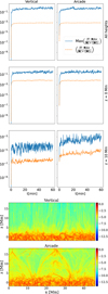 |
Fig. 9 Dimensionless error associated with the divergence of the magnetic field, defined as |∇ ∙ B|∆x/(|B| + 〈|B|〉h). The top three panels show the maximum and average values of this error as functions of time. The left panels correspond to the simulation with an initially vertical magnetic field, while the right panels show the results for the arcade magnetic field configuration. The first row presents values computed over the entire domain, while the second and third rows show values at heights of z=0 Mm and z =10 Mm, respectively. The bottom color maps display the error in logarithmic scale for both simulations for t=2800 s. |
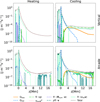 |
Fig. 10 Horizontally and temporally averaged heating and cooling contributions to the internal energy equation as a function of height. The plotted terms are the radiative terms Qloss(orange), Qrad(blue), divergence of heat flux (∇ ∙ q) (green), joule heating from numerical resistivity (ηnum J2, (red)), dissipation from numerical viscosity (∇ ∙ (Πnum ∙ v)), (violet), adiabatic heating (p∇ ∙ v), (navy blue), and flux of internal energy (∇ ∙ (eintv)), (light green). Left panels show heating terms, and right panels show cooling terms. The top row corresponds to the simulation with a vertical magnetic field (Simulation 2), while the bottom row corresponds to the simulation with an arcade-like magnetic field (Simulation 3). The black dotted line in each panel represents the total contribution (sum of all terms). For clarity, values smaller than 1 × 10⁻¹⁰ are omitted from the plots. |
3.2.3 Effects of the perpendicular thermal conductivity
The thermal conductivity model used in our simulations is based on the formulation by Braginskii, as discussed in Section 2.3. However, many similar studies adopt the model developed by Spitzer, which neglects the perpendicular component of thermal conduction. Although this simplification is often justified, we hypothesize that the perpendicular component may still play a non-negligible role in energy transport under certain conditions.
To assess the significance of this effect, we conducted Simulation 4, which uses the Spitzer thermal conduction model. This simulation employs the same setup as the arcade-like magnetic field configuration of Simulation 3. Animations illustrating the time evolution of density and temperature for Simulation 4 are provided in Table 1. Overall, the simulation behaves similarly to Simulation 3, though some differences are worth noting.
Figure 11 shows the difference in horizontally and time-averaged temperature between simulations 3 and 4 over the final 20 minutes of the runs. The vertical bars represent the propagated standard deviation, providing an estimate of the uncertainty. Although the differences may not be statistically significant, they suggest that distinct physical behavior is occurring between the two simulations.
To further check on the origin of these differences, Figure 12 compares temperature color maps between the two simulations in selected zoomed-in regions at different times. The first column of plots corresponds to the simulation with the Braginskii model and the right column to the Spitzer model. Each row represents a snapshot at a different simulation time: from top to bottom-t = 1606, 1613, 2065, 2065, 2075, and 2085 s.
These comparisons reveal localized differences in temperature structure between the two models during magnetic reconnection events near the top boundary, where null points are formed. Although individually small, the cumulative effect of many such events likely explains the differences seen in the time-averaged temperature profile in Figure 11.
From an analytical point of view, this behavior is expected. Eq. (16) shows how the perpendicular component of thermal conduction becomes comparable to the parallel component when the magnetic field strength approaches zero, as occurs at null points formed during reconnection. Therefore, while the impact of the perpendicular conductivity is limited in most regions, it becomes relevant in localized areas of magnetic reconnection.
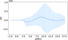 |
Fig. 11 Difference in horizontally and temporally averaged temperature between simulations using Braginskii and Spitzer heat flux models during the final 20 minutes of the simulation. Vertical error bars indicate the propagated standard deviation. |
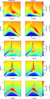 |
Fig. 12 Comparison of the temperature color map at selected snapshots for simulations with different heat flux models. The left column corresponds to the Braginskii model and the right to the Spitzer model. Each row represents a different time: from top to bottom —1=1606 s, t=1613 s, t=2065 s, t=2075 s, and t=2085 s. |
4 Discussion and conclusions
We have introduced the new MAGEC code, providing a detailed description of its numerical methods, as well as its physical modules for thermal conduction and coronal radiative losses. We have also presented the methodology used to estimate the effective numerical resistivity and viscosity. To evaluate the performance and accuracy of the code, we carried out a series of simulations of the solar atmosphere. These simulations serve to demonstrate the robustness and capabilities of MAGEC as a reliable and versatile numerical tool for solar physics research.
In these simulations, we investigated how the inclination of the magnetic field influences the thermal structure of the solar atmosphere. Our results show that a vertical magnetic field configuration sustains a hotter corona at intermediate heights compared to an arcade-like configuration. The stability of our models achieved by the inclusion of a hot plate at the boundary top reinforces the well-established conclusion that an additional heating mechanism is required to maintain coronal temperatures. These findings are consistent with results obtained from other widely used simulation codes.
Through a detailed analysis of the energy equation - including both explicit and implicit contributions - we found that, although numerical resistivity appears dominant in time-averaged heating profiles, its effects are concentrated primarily in the photosphere and chromosphere. In contrast, within the corona, the dominant energy transport mechanisms are thermal conduction and pressure work. The interplay of various heating and cooling processes across different atmospheric layers leads to a complex thermal structure, with alternating regions of net heating and net cooling.
We also examined the role of the perpendicular component of thermal conduction, which is often neglected in coronal models. By comparing simulations using the Braginskii and Spitzer conductivity formulations, we found that while the overall temperature profiles are broadly similar, the perpendicular component can influence local plasma dynamics, especially in the vicinity of magnetic reconnection events. When such events occur frequently, the cumulative effect of these localized differences can become apparent in the average temperature profile.
Although numerous MHD codes have been developed for solar physics, and several of them employ HRSC methods, we are some of the first to use these techniques to model both the near-surface solar interior and the atmosphere in the same computational box. Our approach uniquely incorporates key coronal physical processes, such as optically thin radiative losses and anisotropic thermal conduction, enabling more realistic and self-consistent modeling of the coupled solar interior-corona system. In future work, we plan to extend its capabilities to fully three-dimensional simulations and incorporate additional physical effects, including ambipolar diffusion, the Hall effect, and the Biermann battery.
Data availability
Movies associated to Fig. 5 and Table 1 are available at https://www.aanda.org.
Acknowledgements
This research was funded by the Agencia Estatal de Investigación del Ministerio de Ciencia, Innovación y Universidades (MCIU/AEI) and the European Regional Development Fund (ERDF) under grant “MHD MODeling and beyond: in preparation for the European Solar Telescope” with reference PID2021-127487NB-I00 and by the MCIU/AEI and the European Social Fund (ESF) under grant “Ayudas Ramón y Cajal Convocatoria 2020” with reference RYC2020-030307-I. It also contributes to the deliverables outlined in the FP7 European Research Council grant agreement ERC-2017-CoG771310-PI2FA for the project “Partial Ionization: Two-fluid Approach”. TF acknowledges support from the Project CNS2023-145233, funded by MICIU/AEI/10.13039/501100011033, and the European Union “NextGenera-tionEU/RTRP”. AN gratefully acknoweledges financial support from grant PID2024-156538NB-I00, funded by MCIN/AEI/10.13039/501100011033 and by “ERDF A way of making Europe”. The authors also acknowledge the technical support and expertise provided by the Spanish Supercomputing Network (Red Española de Supercomputación). Computational resources were provided by the LaPalma Supercomputer at the Instituto de Astrofísica de Canarias and the MareNostrum Supercomputer in Barcelona, Spain.
References
- Abbett, W. P. 2007, ApJ, 665, 1469 [Google Scholar]
- Abdel-Hamid, B. 1999, Appl. Math. Model., 23, 899 [CrossRef] [Google Scholar]
- Anders, E., & Grevesse, N. 1989, Geochim. Cosmochim. Acta, 53, 197 [Google Scholar]
- Arber, T. D., Longbottom, A. W., Gerrard, C. L., & Milne, A. M. 2001, J. Comput. Phys., 171, 151 [NASA ADS] [CrossRef] [Google Scholar]
- Braginskii, S. I. 1965, Rev. Plasma Phys., 1, 205 [Google Scholar]
- Canivete Cuissa, J. R., & Teyssier, R. 2022, A&A, 664, A24 [Google Scholar]
- Carlsson, M., Hansteen, V. H., & Gudiksen, B. V. 2010, Mem. Soc. Astron. Italiana, 81, 582 [Google Scholar]
- Cattaneo, C. 1958, Comptes rendus de l’Académie des Sciences, 247, 431 [Google Scholar]
- Cherry, G., Szydlarski, M., & Gudiksen, B. 2024, A&A, 692, A139 [NASA ADS] [CrossRef] [EDP Sciences] [Google Scholar]
- Chiavassa, A., Kravchenko, K., & Goldberg, J. A. 2024, Living Rev. Comput. Astrophys., 10, 2 [CrossRef] [Google Scholar]
- Delorme, M., Durocher, A., Sacha Brun, A., et al. 2025, in J. Phys.: Conf. Ser., 2997, J. Phys.: Conf. Ser. (IOP), 012014 [Google Scholar]
- Dere, K. P., Del Zanna, G., Young, P. R., & Landi, E. 2023, ApJS, 268, 52 [NASA ADS] [CrossRef] [Google Scholar]
- Evans, C. R., & Hawley, J. F. 1988, ApJ, 332, 659 [Google Scholar]
- Freytag, B. 2013, Mem. Soc. Astron. Ital. Suppl., 24, 26 [Google Scholar]
- Freytag, B. 2017, Mem. Soc. Astron. Italiana, 88, 12 [NASA ADS] [Google Scholar]
- González-Avilés, J. J., Cruz-Osorio, A., Lora-Clavijo, F. D., & Guzmán, F. S. 2015, MNRAS, 454, 1871 [Google Scholar]
- Gottlieb, S., Shu, C.-W., & Tadmor, E. 2001, SIAM Rev., 43, 89 [NASA ADS] [CrossRef] [Google Scholar]
- Gudiksen, B. V., Carlsson, M., Hansteen, V. H., et al. 2011, A&A, 531, A154 [NASA ADS] [CrossRef] [EDP Sciences] [Google Scholar]
- Hansteen, V. H., Carlsson, M., & Gudiksen, B. 2007, in ASP Conf. Ser., 368, The Physics of Chromospheric Plasmas, eds. P. Heinzel, I. Dorotovic, & R. J. Rutten, 107 [Google Scholar]
- Harten, A., Lax, P. D., & van Leer, B. 1983, SIAM Rev., 25, 35 [Google Scholar]
- Iijima, H., Matsumoto, T., Hotta, H., & Imada, S. 2023, ApJ, 951, L47 [NASA ADS] [CrossRef] [Google Scholar]
- Jacoutot, L., Kosovichev, A. G., Wray, A., & Mansour, N. N. 2008, ApJ, 684, L51 [NASA ADS] [CrossRef] [Google Scholar]
- Keppens, R., Popescu Braileanu, B., Zhou, Y., et al. 2023, A&A, 673, A66 [NASA ADS] [CrossRef] [EDP Sciences] [Google Scholar]
- Khomenko, E., Vitas, N., Collados, M., & de Vicente, A. 2018, A&A, 618, A87 [NASA ADS] [CrossRef] [EDP Sciences] [Google Scholar]
- Li, S. 2005, J. Comput. Phys., 203, 344 [NASA ADS] [CrossRef] [Google Scholar]
- Lora-Clavijo, F. D., Cruz-Osorio, A., & Guzmán, F. S. 2015, ApJS, 218, 24 [NASA ADS] [CrossRef] [Google Scholar]
- Martínez-Sykora, J., De Pontieu, B., Carlsson, M., et al. 2017, ApJ, 847, 36 [Google Scholar]
- Martínez-Sykora, J., Leenaarts, J., De Pontieu, B., et al. 2020, ApJ, 889, 95 [Google Scholar]
- Mignone, A., Bodo, G., Massaglia, S., et al. 2007, ApJS, 170, 228 [Google Scholar]
- Mihalas, D. 1967, ApJ, 149, 169 [NASA ADS] [CrossRef] [Google Scholar]
- Miyoshi, T., & Kusano, K. 2005, J. Comput. Phys., 208, 315 [NASA ADS] [CrossRef] [Google Scholar]
- Modestov, M., Khomenko, E., Vitas, N., et al. 2024, Sol. Phys., 299, 23 [NASA ADS] [CrossRef] [Google Scholar]
- Murawski, K., Musielak, Z. E., Poedts, S., Srivastava, A. K., & Kadowaki, L. 2022, Ap&SS, 367, 111 [NASA ADS] [CrossRef] [Google Scholar]
- Navarro, A., Lora-Clavijo, F. D., & González, G. A. 2017, ApJ, 844, 57 [NASA ADS] [CrossRef] [Google Scholar]
- Navarro, A., Murawski, K., Wójcik, D., & Lora-Clavijo, F. D. 2019, MNRAS, 489, 2769 [Google Scholar]
- Navarro, A., Lora-Clavijo, F. D., Murawski, K., & Poedts, S. 2021, MNRAS, 500, 3329 [Google Scholar]
- Navarro, A., Khomenko, E., Modestov, M., & Vitas, N. 2022, A&A, 663, A96 [NASA ADS] [CrossRef] [EDP Sciences] [Google Scholar]
- Nordlund, A. 1982, A&A, 107, 1 [Google Scholar]
- Olson, G. L., & Kunasz, P. B. 1987, J. Quant. Spec. Radiat. Transf., 38, 325 [NASA ADS] [CrossRef] [Google Scholar]
- Pencil Code Collaboration (Brandenburg, A., et al.) 2021, JOSS, 6, 2807 [CrossRef] [Google Scholar]
- Popovas, A. 2025, A&A, 698, A69 [NASA ADS] [CrossRef] [EDP Sciences] [Google Scholar]
- Rembiasz, T., Obergaulinger, M., Cerdá-Durán, P., Aloy, M.-Á., & Müller, E. 2017, ApJS, 230, 18 [Google Scholar]
- Rempel, M. 2017, ApJ, 834, 10 [Google Scholar]
- Roe, P. L. 1986, Annu. Rev. Fluid Mech., 18, 337 [NASA ADS] [CrossRef] [Google Scholar]
- Schaffenberger, W., Wedemeyer-Böhm, S., Steiner, O., & Freytag, B. 2005, in ESA Special Publication, Vol. 596, Chromospheric and Coronal Magnetic Fields, eds. D. E. Innes, A. Lagg, & S. A. Solanki, 65.1 [Google Scholar]
- Skála, J., Baruffa, F., Büchner, J., & Rampp, M. 2015, A&A, 580, A48 [NASA ADS] [CrossRef] [EDP Sciences] [Google Scholar]
- Snodin, A. P., Brandenburg, A., Mee, A. J., & Shukurov, A. 2006, MNRAS, 373, 643 [Google Scholar]
- Spitzer, L. 1956, Physics of Fully Ionized Gases (Interscience Publishers) [Google Scholar]
- Spruit, H. C. 1974, Sol. Phys., 34, 277 [Google Scholar]
- Stein, R. F., & Nordlund, Å. 1998, ApJ, 499, 914 [Google Scholar]
- Stein, R. F., & Nordlund, Å. 2006, ApJ, 642, 1246 [NASA ADS] [CrossRef] [Google Scholar]
- Steiner, O., Grossmann-Doerth, U., Knölker, M., & Schüssler, M. 1998, ApJ, 495, 468 [NASA ADS] [CrossRef] [Google Scholar]
- Stone, J. M., Gardiner, T. A., Teuben, P., Hawley, J. F., & Simon, J. B. 2008, ApJS, 178, 137 [NASA ADS] [CrossRef] [Google Scholar]
- Titarev, V. A., & Toro, E. F. 2004, J. Comput. Phys., 201, 238 [Google Scholar]
- Toriumi, S., Hotta, H., & Kusano, K. 2024, ApJ, 975, 209 [Google Scholar]
- Toro, E. F. 2009, Riemann Solvers and Numerical Methods for Fluid Dynamics (Springer) [Google Scholar]
- van Leer, B. 1974, J. Comput. Phys., 14, 361 [NASA ADS] [CrossRef] [Google Scholar]
- Van Leer, B. 1977, J. Comput. Phys., 23, 263 [NASA ADS] [CrossRef] [Google Scholar]
- Vernazza, J. E., Avrett, E. H., & Loeser, R. 1981, ApJS, 45, 635 [Google Scholar]
- Vernotte, P. 1958, Compt. Rendu, 246, 3154 [Google Scholar]
- Vitas, N., & Khomenko, E. 2015, Ann. Geophys., 33, 703 [NASA ADS] [CrossRef] [Google Scholar]
- Vögler, A., Shelyag, S., Schüssler, M., et al. 2005, A&A, 429, 335 [Google Scholar]
- Warnecke, J., & Bingert, S. 2020, Geophys. Astrophys. Fluid Dyn., 114, 261 [NASA ADS] [CrossRef] [Google Scholar]
- Waterson, N., & Deconinck, H. 2007, J. Comput. Phys., 224, 182 [Google Scholar]
- Wójcik, D., Murawski, K., & Musielak, Z. E. 2018, MNRAS, 481, 262 [CrossRef] [Google Scholar]
Appendix A Distribution of the heating and cooling terms in the internal energy equation
 |
Fig. A.1 Graphical analysis of the heating and cooling terms from Figure 10 at selected heights. Histograms and pie charts represent the contributions of the heating and cooling terms in the internal energy equation at z = 10, 6, 3, 1, 0, −1 Mm. The left column of plots corresponds to the simulation with a vertical magnetic field, and the right column to the simulation with an arcade-like magnetic field. Each histogram is accompanied by two pie charts illustrating the relative contributions of the individual terms to the total heating and cooling. |
All Tables
All Figures
|
Fig. 1 Density-averaged radiative loss rate Λ(T) from the CHIANTI 10.1 database with photospheric abundances. |
| In the text | |
|
Fig. 2 Graphical estimation of numerical resistivity (top panel) and numerical viscosity (bottom panel). Each dot represents the maximum magnetic field (Bmax) or velocity (Vmax) obtained from a simulation with a specific explicit value of η or ν. The blue solid line is a fit to these data points. Two horizontal lines are shown: one corresponds to the Bmax/Vmax value for the case with η = 0 and ν = 0, and the other marks the threshold of numerical noise. The intersection of this threshold with the fitted curve defines the estimated numerical resistivity or viscosity, indicated by the vertical line. |
| In the text | |
|
Fig. 3 Initial profiles of density and temperature as functions of height. |
| In the text | |
|
Fig. 4 Initial plasma-beta profiles as a function of height, evaluated at the center of the domain in the x-direction, for both the vertical and arcade magnetic field configurations after field implantation. |
| In the text | |
|
Fig. 5 Color map of the temperature from the baseline hydrodynamic simulation at t = 1000 s. Arrows indicate the velocity field, with lengths proportional to the local flow speed. The associated movie is available online. |
| In the text | |
|
Fig. 6 Color map of the magnetic field strength in gauss and field line configuration of the arcade-like model. |
| In the text | |
|
Fig. 7 Color map of the logarithmic temperature distribution after 1 hour of solar time. The top panel shows the simulation with a vertical magnetic field (Simulation 2), and the bottom panel shows the simulation with an arcade-like magnetic field (Simulation 3). The arrows indicate the velocity field, with lengths proportional to the local flow speed, bthe blacklines are magnetic field lines. |
| In the text | |
|
Fig. 8 Horizontally averaged temperature profiles for the simulations shown in Fig. 7 for the last 20 minutes. The left panel displays the horizontally averaged temperature as a function of height and time, with contour lines overlaid to highlight specific temperature values. The right panel shows the temperature averaged both horizontally and over time. The black dotted line indicates the initial profile. |
| In the text | |
|
Fig. 9 Dimensionless error associated with the divergence of the magnetic field, defined as |∇ ∙ B|∆x/(|B| + 〈|B|〉h). The top three panels show the maximum and average values of this error as functions of time. The left panels correspond to the simulation with an initially vertical magnetic field, while the right panels show the results for the arcade magnetic field configuration. The first row presents values computed over the entire domain, while the second and third rows show values at heights of z=0 Mm and z =10 Mm, respectively. The bottom color maps display the error in logarithmic scale for both simulations for t=2800 s. |
| In the text | |
|
Fig. 10 Horizontally and temporally averaged heating and cooling contributions to the internal energy equation as a function of height. The plotted terms are the radiative terms Qloss(orange), Qrad(blue), divergence of heat flux (∇ ∙ q) (green), joule heating from numerical resistivity (ηnum J2, (red)), dissipation from numerical viscosity (∇ ∙ (Πnum ∙ v)), (violet), adiabatic heating (p∇ ∙ v), (navy blue), and flux of internal energy (∇ ∙ (eintv)), (light green). Left panels show heating terms, and right panels show cooling terms. The top row corresponds to the simulation with a vertical magnetic field (Simulation 2), while the bottom row corresponds to the simulation with an arcade-like magnetic field (Simulation 3). The black dotted line in each panel represents the total contribution (sum of all terms). For clarity, values smaller than 1 × 10⁻¹⁰ are omitted from the plots. |
| In the text | |
|
Fig. 11 Difference in horizontally and temporally averaged temperature between simulations using Braginskii and Spitzer heat flux models during the final 20 minutes of the simulation. Vertical error bars indicate the propagated standard deviation. |
| In the text | |
|
Fig. 12 Comparison of the temperature color map at selected snapshots for simulations with different heat flux models. The left column corresponds to the Braginskii model and the right to the Spitzer model. Each row represents a different time: from top to bottom —1=1606 s, t=1613 s, t=2065 s, t=2075 s, and t=2085 s. |
| In the text | |
|
Fig. A.1 Graphical analysis of the heating and cooling terms from Figure 10 at selected heights. Histograms and pie charts represent the contributions of the heating and cooling terms in the internal energy equation at z = 10, 6, 3, 1, 0, −1 Mm. The left column of plots corresponds to the simulation with a vertical magnetic field, and the right column to the simulation with an arcade-like magnetic field. Each histogram is accompanied by two pie charts illustrating the relative contributions of the individual terms to the total heating and cooling. |
| In the text | |
Current usage metrics show cumulative count of Article Views (full-text article views including HTML views, PDF and ePub downloads, according to the available data) and Abstracts Views on Vision4Press platform.
Data correspond to usage on the plateform after 2015. The current usage metrics is available 48-96 hours after online publication and is updated daily on week days.
Initial download of the metrics may take a while.