| Issue |
A&A
Volume 703, November 2025
|
|
|---|---|---|
| Article Number | A251 | |
| Number of page(s) | 18 | |
| Section | Planets, planetary systems, and small bodies | |
| DOI | https://doi.org/10.1051/0004-6361/202556257 | |
| Published online | 26 November 2025 | |
Atmospheric composition and circulation of the ultra-hot Jupiter WASP-121b with joint NIRPS, HARPS and CRIRES+ transit spectroscopy
1
Observatoire de Genève, Département d’Astronomie, Université de Genève,
Chemin Pegasi 51,
1290
Versoix,
Switzerland
2
Institut Trottier de recherche sur les exoplanètes, Département de Physique, Université de Montréal,
Montréal,
Québec,
Canada
3
Centre Vie dans l’Univers, Faculté des sciences de l’Université de Genève,
Quai Ernest-Ansermet 30,
1205
Geneva,
Switzerland
4
Light Bridges S.L., Observatorio del Teide,
Carretera del Observatorio, s/n Guimar,
38500,
Tenerife,
Canarias,
Spain
5
Instituto de Astrofísica de Canarias (IAC),
Calle Vía Láctea s/n,
38205
La Laguna,
Tenerife,
Spain
6
Departamento de Astrofísica, Universidad de La Laguna (ULL),
38206
La Laguna,
Tenerife,
Spain
7
Division of Astrophysics, Department of Physics, Lund University,
Box 118,
SE-22100
Lund,
Sweden
8
Observatoire du Mont-Mégantic,
Québec,
Canada
9
Instituto de Astrofísica e Ciências do Espaço, Universidade do Porto,
CAUP, Rua das Estrelas,
4150-762
Porto,
Portugal
10
Departamento de Física e Astronomia, Faculdade de Ciências, Universidade do Porto,
Rua do Campo Alegre,
4169-007
Porto,
Portugal
11
Department of Earth, Planetary, and Space Sciences, University of California,
Los Angeles,
CA
90095,
USA
12
Univ. Grenoble Alpes, CNRS, IPAG,
38000
Grenoble,
France
13
Department of Physics, University of Toronto,
Toronto,
ON
M5S 3H4,
Canada
14
Departamento de Física Teórica e Experimental, Universidade Federal do Rio Grande do Norte,
Campus Universitário,
Natal,
RN
59072-970,
Brazil
15
Department of Physics & Astronomy, McMaster University,
1280 Main St W,
Hamilton,
ON
L8S 4L8,
Canada
16
Department of Physics, McGill University,
3600 rue University,
Montréal,
QC
H3A 2T8,
Canada
17
Department of Earth & Planetary Sciences, McGill University,
3450 rue University,
Montréal,
QC
H3A 0E8,
Canada
18
Centro de Astrobiología (CAB), CSIC-INTA,
Camino Bajo del Castillo s/n,
28692,
Villanueva de la Cañada (Madrid),
Spain
19
European Southern Observatory (ESO),
Karl-Schwarzschild-Str. 2,
85748
Garching bei München,
Germany
20
Space Research and Planetary Sciences, Physics Institute, University of Bern,
Gesellschaftsstrasse 6,
3012
Bern,
Switzerland
21
Consejo Superior de Investigaciones Científicas (CSIC),
28006
Madrid,
Spain
22
Bishop’s Univeristy, Department of Physics and Astronomy,
Johnson-104E, 2600 College Street,
Sherbrooke,
QC
J1M 1Z7,
Canada
23
Department of Physics, Engineering Physics, and Astronomy, Queen’s University,
99 University Avenue,
Kingston,
ON
K7L 3N6,
Canada
24
Department of Physics and Space Science, Royal Military College of Canada,
13 General Crerar Cres.,
Kingston,
ON
K7P 2M3,
Canada
25
School of Mathematical and Physical Sciences, Macquarie University,
Sydney,
NSW
2109,
Australia
26
Lund Observatory, Division of Astrophysics, Department of Physics, Lund University,
Box 118,
221 00
Lund,
Sweden
27
European Southern Observatory (ESO),
Av. Alonso de Cordova 3107,
Casilla
19001,
Santiago de Chile,
Chile
28
Université Côte d’Azur, Observatoire de la Côte d’Azur, CNRS, Laboratoire Lagrange,
06000
Nice,
France
29
Institute of Space Sciences (ICE, CSIC),
Carrer de Can Magrans S/N, Campus UAB,
Cerdanyola del Valles
08193,
Spain
30
Institut d’Estudis Espacials de Catalunya (IEEC),
08860
Castellde-fels (Barcelona),
Spain
★ Corresponding author: This email address is being protected from spambots. You need JavaScript enabled to view it.
Received:
4
July
2025
Accepted:
26
August
2025
Abstract
Ultra-hot gas giants such as WASP-121b provide unique laboratories for exploring atmospheric chemistry and dynamics under extreme irradiation conditions. Uncovering their chemical composition and atmospheric circulation is critical for tracing planet formation pathways. Here, we present a comprehensive atmospheric characterisation of WASP-121b using high-resolution transit spectroscopy across the optical to infrared with HARPS, NIRPS, and CRIRES+ spanning nine transit events. These observations are complemented with five TESS photometric sectors, two EulerCam light curves simultaneous to the HARPS and NIRPS transits, and an extensive radial velocity dataset in order to refine WASP-121b's orbital parameters. A cross-correlation analysis detected iron (Fe), carbon monoxide (CO) and vanadium (V) absorption signals with SNR of 5.8, 5.0, and 4.7, respectively. Our retrieval analysis constrains the water (H2O) abundance to −6.52−0.68+0.49 dex, although its absorption signal is effectively muted by the hydride (H−) continuum. We constrained the relative abundances of the volatile and refractory elements - which represents a crucial diagnostic of atmospheric chemistry, evolution, and planet formation pathways. The retrieved abundance ratios are broadly consistent with expected values of a solar composition atmosphere in chemical equilibrium, likely indicating minimal disequilibrium chemistry alterations at the probed pressures (∼10−4−10−3 bar). We update the orbital parameters of WASP-121b with its largest radial velocity dataset to date. By comparing orbital velocities derived from both the radial velocity analysis and the atmospheric retrieval, we determined a non-zero velocity offset caused by atmospheric circulation, ΔKp = −15 ± 3 km s−1 (assuming M⋆ = 1.38 ± 0.02 M⊙), consistent with predictions from either drag-free or weak-drag 3D global circulation models, while we caution the non-negligible dependence on the assumed stellar mass. These results place new constraints on the thermal structure, dynamics, and chemical inventory of WASP-121b, highlighting the power of multi-wavelength high-resolution spectroscopy to probe exoplanetary atmospheres.
Key words: instrumentation: spectrographs / methods: observational / techniques: spectroscopic / planets and satellites: atmospheres / planets and satellites: composition / planets and satellites: gaseous planets
© The Authors 2025
 Open Access article, published by EDP Sciences, under the terms of the Creative Commons Attribution License (https://creativecommons.org/licenses/by/4.0), which permits unrestricted use, distribution, and reproduction in any medium, provided the original work is properly cited.
This article is published in open access under the Subscribe to Open model. This email address is being protected from spambots. You need JavaScript enabled to view it. to support open access publication.
1 Introduction
Ultra-hot Jupiters represent the hottest class of gas giant exoplanets (Teq > 2000 K), showcasing extreme atmospheric conditions driven by the proximity to their hot, early-type (typically A or F) host star (e.g. Hellier et al. 2009; Collier Cameron et al. 2010; West et al. 2016; Delrez et al. 2016; Gaudi et al. 2017; Lund et al. 2017; Anderson et al. 2018). These planets receive an enormous amount of stellar irradiation that is orders of magnitude larger than what is observed in Solar-system planets. Importantly, it drives the thermal dissociation of molecules and the ionisation of atoms (Kitzmann et al. 2018; Parmentier et al. 2018; Hoeijmakers et al. 2018, 2019), atmospheric circulations (Arcangeli et al. 2019; Seidel et al. 2019, 2020a, 2021; Seidel et al. 2025), heat transport through the dissociation and recombination of molecular hydrogen (H2; Bell & Cowan 2018; Tan & Komacek 2019), and condensation of metals on the nightside (Ehrenreich et al. 2020; Gandhi et al. 2023; Pelletier et al. 2023). At such elevated temperatures, not only do new spectral features appear, but lines already present at lower temperatures also have their amplitude and width bolstered. This overall increase in the line strength relative to the continuum makes ultra-hot gas giants ideal targets for atmospheric characterisation via transmission and emission spectroscopy.
High-resolution transmission and emission spectroscopy have proven to be valuable methods to characterise the atmosphere. Ultra-hot Jupiters, in tandem with the cross-correlation technique (e.g. Snellen et al. 2010; Brogi et al. 2012; Birkby et al. 2013; Hoeijmakers et al. 2018, 2019, 2020a; Ehrenreich et al. 2020; Prinoth et al. 2022, 2023; Prinoth et al. 2025; Vaulato et al. 2025). The cross-correlation method has been broadly used to infer the chemical composition of planetary atmospheres as well as their dynamics (Seidel et al. 2020b; Seidel et al. 2025; Wardenier et al. 2024; Ramkumar et al. 2025) by resolving individual spectral lines of broad molecular bands and measuring the planet’s Doppler shift at the level of km s−1 precisions. Unlike low-resolution spectroscopy, high-resolution data are typically self-calibrated by removing broadband flux variations and temporal changes in flux at each wavelength, and thus they lack reliable information on the planet’s continuum, see however Santos et al. (2020). Cross-correlation is then limited in the sense of being insensitive to residual broadband variations. Brogi & Line (2019) have introduced a statistically robust atmospheric retrieval framework to overcome such limitations and access the chemical composition and temperature-pressure profile of planetary atmospheres.
Discovered by Delrez et al. (2016), WASP-121b is a benchmark ultra-hot Jupiter target (Rp = 1.753 ± 0.036 RJ, Mp = 1.157 ± 0.070 MJ, Porb ~ 1.27 days, T = 2358 ± 52 K; Delrez et al. 2016; Bourrier et al. 2020; Patel & Espinoza 2022) in an highly misaligned orbit (λ = 87.20 deg, Bourrier et al. 2020) around its F6V-type star. It has been extensively observed in both emission and transmission across a broad range of wavelengths in low and high-resolution (e.g. Evans et al. 2016; Hoeijmakers et al. 2020b; Sing et al. 2024; Seidel et al. 2025; Gapp et al. 2025).
Exospheric species such as excited hydrogen (Hα) and ionised iron (Fe II) and calcium (Ca II) (firstly detected at high altitudes by Sing et al. 2019; Borsa et al. 2021) have been found to extend beyond the Roche limit, which implies that implies the planet experiences mass loss. The 4-UT VLT/ESPRESSO (Pepe et al. 2021) partial transit data obtained during the commissioning of the spectrograph (Borsa et al. 2021) were also used in Seidel et al. (2023) to interpret the blue-shifted sodium feature (firstly identified by Hoeijmakers et al. 2020b) as a signature of equatorial day-to-nightside winds crossing the evening limb. In particular, Seidel et al. (2023) characterised the secondary Na feature visible only in egress, and they found that it was far more offset. Maguire et al. (2023) constrained the relative abundances of metals by stacking high-resolution optical spectra obtained with ESPRESSO. They used two transits in the 1-UT mode and an archival partial transit in the 4-UT mode from the commissioning data (i.e. the same data used by Borsa et al. 2021 and Seidel et al. 2023), and they retrieved abundance ratios generally consistent with stellar values, albeit with some exceptions. Further insights into atmospheric dynamics were gained through phase-resolved infrared transmission spectra from Gemini-S/IGRINS (Park et al. 2014). Carbon monoxide and H2O were detected and interpreted with 3D global circulation models (GCM; Wardenier et al. 2024), thus suggesting the importance of atmospheric drag. A new 4-UT ESPRESSO dataset, completing the partial transit reported in Borsa et al. (2021), Seidel et al. (2023), and Maguire et al. (2023) allowed Seidel et al. (2025) to unveil an onion-layered upper atmosphere. In this configuration (see their Figure 3), atomic iron (Fe I) traces sub-to-antistellar flows (day-to-night winds) at approximately millibar pressures; sodium (Na I) probes jet streams from the morning to evening terminator at lower pressures (−10−5 bar), and the hydrogen ions (HI) track the remarkably red- to blue-shifted signature of the jet at very high altitudes (-10−6 bar).
In the context of atmospheric characterisation, Hoeijmakers et al. (2024) reported on significant detections (earlier reported by Hoeijmakers et al. 2020b) of atomic calcium (Ca I), vanadium (V I), chromium (Cr I), manganese (Mn I), iron (Fe I), cobalt (Co I), and nickel (Ni I) in ESPRESSO dayside spectra, while atomic titanium (Ti I) and titanium oxide (TiO) were notably not detected in cross-correlation. These authors surmised that Ti-bearing species condense on the nightside and remain cold-trapped there, so they are thus inaccessible to both transmission and emission spectroscopy. Merritt et al. (2021) used VLT/UVES (Dekker et al. 2000) transit time series to confirm robust detections of Fe I, Cr I, V I, Ca I, K I and exospheric H I and Ca II while adding a novel detection of ionised scandium (Sc II). However, Prinoth et al. (2025), leveraging the high signal-to-noise ratio of 4-UT ESPRESSO transit observations, successfully detected titanium (Ti), but they found the signal to be notably weaker than expected. Meanwhile, titanium oxide (TiO) still remains undetected, likely due to limitations in the current line lists. Additionally, Prinoth et al. (2025) reported a plethora of detected species (i.e. neutral atoms such as H I, Li I, Na I, Mg I, K I, Ca I, Ti I, Cr I, Mn I, and Fe I as well as excited atoms such as V II, Fe II, Co I, Ni I, Ba II, Sr I, and Sr II), thus confirming and expanding on previous literature findings (Merritt et al. 2021; Silva et al. 2022; Hoeijmakers et al. 2024). Optical (ESPRESSO) and infrared (VLT/CRIRES+; Dorn et al. 2023) data were used by Pelletier et al. (2024) to measure the volatile-to-refractory budget and C/O ratio. An analogue study was carried out in Smith et al. (2024) using IGRINS data. Overall, similar properties for the dayside atmosphere of WASP-121b were retrieved, but the authors arrived at contrasting conclusions regarding the atmospheric volatile-to-refractory enrichment. Indeed, Pelletier et al. (2024) concluded that the atmosphere of WASP-121b is likely volatile rich, while Smith et al. (2024) preferred a super-stellar refractory-to-volatile ratio, despite both finding a C/O ~ 0.70 under the assumption of chemical equilibrium conditions. On this topic, a recent work by Evans-Soma et al. (2025) reports on super-stellar C/H, O/H and C/O ratios (along with robust water, carbon monoxide, and silicon monoxide detections) obtained with a single JWST observation, suggesting that pebbles and planetesimal are important in the formation pathway of giant planets. Among the latest published results, the Near-Infrared Planet Searcher (NIRPS; Bouchy et al. 2025) has confidently detected both H2O and its thermal dissociation byproduct, OH, in the thermal spectrum of WASP-121b, providing evidence for water dissociation that aligns with model predictions (Bazinet et al. 2025).
In this paper, we report on the first near-infrared highresolution spectroscopic NIRPS observations of WASP-121b’s transit, which we combine with simultaneous HARPS and archival CRIRES+ transit time series. The scientific objective is to characterise the chemical composition and the ongoing chemical processes in WASP-121b’s atmosphere. Furthermore, we complement the spectroscopic data with high-precision radial velocity (RV) measurements in order to refine the orbital parameters of the system.
In Section 2, we describe the spectroscopic and photometric observations. Section 3 presents a global fit to the RVs and photometry in order to improve the planetary parameters, particularly the RV semi-amplitude. It includes five TESS sectors, and a total of 1261 public RV measurements from CORALIE, HARPS, ESPRESSO, and NIRPS. We note that this is the largest RV dataset ever used to characterise WASP-121 b. Section 4 illustrates the data processing for atmospheric analyses, the cross-correlation approach, and the atmospheric retrieval recipe. In Section 5, we discuss the detections of cross-correlation functions, describe the key retrieval results, and compare the findings with previous results in the context of global circulation models, and discuss their implications.
Log of NIRPS, HARPS and CRIRES+ transit observations.
2 Observations
2.1 Spectroscopic transit observations with NIRPS and HARPS
We observed a total of four transits of WASP-121b across the disc of its relatively bright host star WASP-121 (V=10.51, J=9.63; Høg et al. 2000; Cutri et al. 2003, respectively) simultaneously with the high-resolution spectrographs HARPS (Pepe et al. 2000) and the new fiber-fed, ultra stable and high-precision Near-Infrared Planet Searcher (NIRPS; Bouchy et al. 2025). NIRPS has been designed (i) to expand the wavelength coverage from the optical to the Y, J, and H bands, (ii) to leverage avantgarde adaptive optics, and (iii) to operate simultaneously with HARPS at the 3.6-m telescope in La Silla, Chile. We observed WASP-121b transits on 2023-01-24 (Night 1) and 2023-03-02 (Night 2) as part of the commissioning (program ID 60.A-9109) of the NIRPS instrument, and on 2023-12-15 (Night 3) and 2025-01-21 (Night 4) as part of the ESO GTO program IDs 112.25P3.001 and 112.25P3.003, respectively (PI: F. Bouchy). Of those, three transit observations (i.e. Nights 2, 3, and 4) have been gathered simultaneously with HARPS in High Accuracy Mode (HAM) and NIRPS in High Efficiency (HE, Night 3 and 4) and High Accuracy (HA, Night 2) modes (Bouchy et al. 2025), whereas the first transit was observed with NIRPS only. The transit of WASP-121b has been partially observed by HARPS and NIRPS also on 2025-02-27, but the dataset was discarded and not used in this work because of major technical issues (problems with the hydraulic system causing the dome vignetting the mirror) severely impacting the quality of the data (low signal-to-noise ratio). We refer the reader to Table 1 and Figure 1 for a summary of the observation status.
The transit duration (from the first to the fourth contact) is about 3 hours, and the total observing time (transit duration + baseline before ingress and after egress) was about 5 hours for all transits. All spectra were reduced by the automated HARPS and NIRPS Data Reduction Softwares (DRS version 3.2.5 and 3.2.0, respectively; Pepe et al. 2021), which yield the echelle-order merged (S1D) and echelle-order separated (S2D) spectra corrected for the Barycentric Earth Radial Velocity (BERV). The starting point of the atmospheric analysis are the HARPS and NIRPS S2D_BLAZE_A.fits files, namely the science fiber acquired and neither blaze nor telluric corrected spectra. We thus work on a temporal series of spectra f (λ, t) = f (λ, t)|BERV (i.e. provided in the barycentric rest frame).
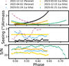 |
Fig. 1 Observing conditions as a function of phase. The blue, orange, yellow, and green points correspond to NIRPS (and simultaneous HARPS) observations, while the pink and black points represent CRIRES+ observations in the H- and K-bands, respectively. Top panel and mid panel illustrate the airmass and the average atmospheric Dimm seeing (i.e. value for the differential image monitor) evolving during the nights, respectively. The Dimm seeing is averaged for each observations (i.e. average between the start and the end of each observation). The bottom panel shows the signal-to-noise ratio (extracted from the fits header) changing during the nights. |
2.2 Spectroscopic transit observations with CRIRES+
We supplement our optical and near-infrared observations with two CRIRES+ transit time series (Night 5 on 2021-12-12, PI: Romain Allart, program ID: 108.22CZ; Night 6 on 2022-04-02, PI: Brian Thorsbro, program ID 109.23D2). CRIRES+ is a highresolution infrared slit spectrograph (Follert et al. 2014; Dorn et al. 2023) installed at UT3 of the Very Large Telescope in Paranal, Chile. The observations are gathered in the K (Night 5) and H (Night 6) spectroscopic bands, respectively. In the K-band, the exposures were taken in the ABBA nodding sequence (alternated position on the slit) to best subtract contributions from sky background sources, while in the H-band they were gathered in an unconventional AAABBBBBBAAA nodding to reduce the time spent on nodding. To preserve a better time sampling and avoid additional blurring of the rapidly accelerating planetary signal, we chose not to perform our analysis on the combined AB spectra, and instead we analysed the A and B output spectra individually. Specifically, we treated the A nodding positions and the B nodding positions as separate time series for both the H and K-band observations. That said, neither the H- nor K-band data were background subtracted, but this is not worrying as background subtraction was performed as part of by the principal component analysis at a later stage of the data reduction pipeline (see Section 4 for details).
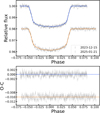 |
Fig. 2 Simultaneous photometry with EulerCam. Top: detrended EulerCam light curves with the best-fit transit models overlaid on top. Bottom: residuals for each observation. The horizontal dashed lines indicate the continuum at zero. |
2.3 Simultaneous photometry with EulerCam
Simultaneously with the NIRPS+HARPS observations on Nights 3 and 4, we acquired two photometric transits using the EulerCam instrument mounted on the ESO 1.2-meter Swiss Euler telescope (Lendl et al. 2012) on UT nights 2023-12-15 and 2025-01-21. The goal of our observations was to refine the ephemerides and to identify and mitigate the impact of any starspot occultations. The observations were taken in Geneva-r and Geneva-v filters with an exposure time of 30 and 45 seconds. The image reduction includes bias, flat and over-scan correction, and the aperture photometry uses the prose framework (Garcia et al. 2022). The optimal differential photometry is performed following Broeg et al. (2005). The transit light curves are modelled using the CONAN package (Lendl et al. 2017). The best-fit transit model along with the detrended light curves is shown in Figure 2. The obtained ephemerides are compatible with Bourrier et al. (2020). Thus, we choose to use the timings derived from Bourrier et al. (2020). Furthermore, we used PyTranSpot (Juvan et al. 2018; Chakraborty et al. 2024) to search for any starspot occultations by simultaneously fitting a transit and spot model. In conclusion, we found no evidence of starspot contamination in the transit light curves.
3 Refined system parameters
In order to refine the orbital solution of WASP-121b, in particular the radial velocity (RV) semi-amplitudes used to calculate the value and uncertainty of ΔKp (see Sect. 5.3), we carry out a simultaneous fit of all available RV datasets and all TESS photometric data with the juliet1 software (Espinoza et al. 2019). juliet uses the radvel package (Fulton et al. 2018) and the batman package (Kreidberg 2015) to model RVs and transits respectively, exploring the parameter space via importance nested sampling with the dynesty package (Speagle 2020). It employs random walk sampling with 500 live points by default. Gaussian processes (GPs) can be incorporated via the celerite package (Foreman-Mackey et al. 2017).
The fit incorporates ten RV datasets and five TESS sectors, which are described in Tables 2 and 3, respectively. We remove all in-transit RVs affected by the Rossiter-McLaughlin effect, but retain the out-of-transit baseline-establishing observations for these datasets, which notably allows us to incorporate three such sets of ESPRESSO data. For the TESS photometry, we use the Presearch Data Conditioning Simple Aperture Photometry (PDC-SAP) light curves (Stumpe et al. 2012, 2014; Smith et al. 2012) generated by the TESS Science Processing Operations Center (SPOC, Jenkins et al. 2016) at NASA Ames Research Center. We obtain the light curves from the Mikulski Archive for Space Telescopes (MAST) archive. The RV data, meanwhile, are obtained from the Data & Analysis Center for Exoplanets (DACE) platform2. The specific data reduction system (DRS) versions used for each dataset, and the median RV errors, are listed in Table 2. We treat datasets from different modes (e.g. NIRPS in high accuracy or high efficiency mode), and/or from before and after instrument upgrades (e.g. the ESPRESSO fibre link replacement, Pepe et al. 2021), as separate instruments for the purposes of this analysis. This allows us to account for any offsets between the datasets.
We pre-detrend the TESS sectors using a GP with the (approximate) Matern 3/2 kernel, as implemented in celerite, via a two-step process where we employ the out-of-transit data to constrain the GP which we then apply to the in-transit data. We first mask the in-transit data in each sector, with a 5h padding of the transit window. Next, we fit a GP to the out-of-transit data in each sector, with broad log-uniform priors of J(1 × 10⁻⁶, 1 × 10⁶) for σGP,sector and J(1 × 10⁻³, 1 × 10³) for ρGP,sector. We also fit the flux offset mflux,sector, and jitter σw,sector for each sector using the out-of-transit data, setting the dilution factor mdilution,sector to 1 for all sectors. We then fix the resulting parameters for the final fit, in which we use only the in-transit data.
We fit the following parameters in the global fit: stellar density p; the period Pb, RV semi-amplitude Kb (i.e. the stellar reflex motion), time of transit t0,b, planet-to-star radius ratio pb, and impact parameter bb for WASP-121b; the systemic RV μinstrument and jitter σw,instrument for each RV instrument; and common limb-darkening parameters q1,TESS and q2,TESS for all TESS sectors. For the limb-darkening parameters, we used the quadratic law parametrisation of Kipping (2013), with uninformative priors of U(0,1). Given the very short period of the planet, we fix the eccentricity to 0. For Pb, t0,b, pb, and bb we use the values of Bourrier et al. (2020) as the central point of normal priors. As we are especially interested in Kb, we take a broad prior of U(0,1000)ms−1. For the systemic radial velocities we set uniform priors between the minimum and maximum RV values for each instrument; for the RV jitter, we set log-uniform priors of J(0.001,100)ms−1. The host star is an active fast rotator, and this activity has previously been reported to affect the RVs, necessitating their detrending (Delrez et al. 2016; Bourrier et al. 2020). For this analysis, we also simultaneously fit a separate GP with the (approximate) Matern 3/2 kernel to each dataset except for the single-night ESPRESSO1, ESPRESSO2, and ESPRESSO5 datasets. These three datasets were excluded because their very short baselines do not allow for a good characterisation of the stellar activity; we also note that preliminary test fits including a GP component for these datasets showed no improvement in their RV dispersion. To constrain the GP parameters, we first fit a GP to the FWHM activity indicator time series for each dataset, which show significant scatter and structure, similarly to Hobson et al. (2024). We take broad uniform priors of U(1,5000) for σGP and U(0.1,10) for pGP. We then use the posteriors of these fits as normal priors for the RV GPs in the full fit.
The full priors and posteriors are reported in Table 4. We show the RV time series and best-fit model in Figure 3, the phase-folded RVs and model in Fig. 4 and the phase-folded TESS photometry in Fig. 5. We use the fitted stellar RV semi-amplitude Kb =  ms−1 to obtain a planet RV semi-amplitude of Kp = 218.42 ± 1.06kms−1. To compute WASP-121b's orbital velocity semi-amplitude, we use Equation 1 in Torres et al. (2010), which does not depend on the planet mass. The planet mass is measured from the juliet RV fit, thus we prefer not to assume its value a priori to derive the orbital Kp. To calculate the orbital planetary velocity, we assume a stellar mass M⋆ = 1.38 ± 0.02 M⊙ (Borsa et al. 2021), an orbital inclination i = 88.49 ± 0.16° (Bourrier et al. 2020), and a fixed zero eccentricity. However, Kp is directly proportional to the stellar mass which is not easy to extract in the case of F-type stars such as WASP-121 owing to the high stellar activity and fast rotation (see Section 5.3 for an in depth discussion). In this work, we assume the stellar mass extracted by Borsa et al. (2021) (see their Table 2, and Sections 3 and 4), as they relied on the complete 1-UT transit dataset gathered with VLT/ESPRESSO.
The uncertainty on Kp is calculated using error propagation. In this case, Kp depends on the stellar mass, the orbital inclination, the stellar reflex velocity, and the orbital period. To compute the uncertainty on Kp, we use the finite difference method to approximate the partial derivatives. Thus, when including all available RV datasets (Table 2, Figure 4), we improve the uncertainty on both the stellar reflex motion Kb and the computed semi-amplitude orbital velocity of WASP-121b with respect to Bourrier et al. (2020) (see their Table 1).
Radial velocity datasets for the juliet modelling.
TESS datasets for the juliet modelling.
Prior and posterior planetary parameter distributions obtained with juliet for WASP-121.
4 Data processing for atmospheric analyses
We carried out cross-correlation and atmospheric retrieval analyses on the combined HARPS, NIRPS and CRIRES+ transit time series. In order to isolate the planetary signal, the data must first be detrended in order to remove telluric and stellar contributions that dominate the observed spectra. This involves the steps described in Pelletier et al. (2021, 2023), and recapitulated as follow: We apply a σ-clipping to the flux variation and all outliers at more than 6σ are flagged and removed. We also discard those bad exposures affected by residual systematics. Heavily telluric contaminated regions are masked out (e.g., 0.6868-0.694 μm, 1.345-1.4465 μm, 1.7995-1.96 μm). Near-infrared to infrared spectra are notoriously polluted by Earth’s atmospheric emission (i.e. OH) and absorption lines (i.e. H2O, CH4, CO2, O2). An additional mask-clipping is applied to data below 0.5 (considering the spectrum as normalised to one) to mask deep telluric spectral lines outside those highly telluric contaminated regions already discarded. All spectra are adjusted to the same continuum level according to a double filtering approach (Gibson et al. 2020): a first box-filter of width 51 pixels is applied to each exposure, smoothed by a Gaussian convolution with a standard deviation of 100 pixels applied to each individual order. This accounts for continuum variations or blaze variations along the observed time series.
A second order polynomial is used to fit the built out-oftransit median spectrum for one night (done night by night) and then divided from each single exposure to remove first-order stellar or telluric residual lines. The Principal Component Analysis (PCA) routine is employed to remove any telluric lines and stellar residuals in the data and reconstruct the observed spectral temporal series. After testing, we decide to remove 5 principal components to best compromise on the cleanliness of the data while preserving the planetary signal. Finally, all column pixels having a standard deviation greater than 5σ that of the spectral order are masked out. Results of the detrending steps for NIRPS, HARPS, and CRIRES+ transit time series are shown in Figure A.1 in Appendix A.
4.1 Cross-correlation analysis
As described by Vaulato et al. (2025), we use SCARLET (Benneke & Seager 2012, 2013; Benneke 2015; Benneke et al. 2019; Pelletier et al. 2021) to generate synthetic transmission spectra of WASP-121b. SCARLET models use (i) H2-H2 and H2-He collision-induced opacities (Borysow 2002), (ii) molecular cross-sections for H2O (Polyansky et al. 2018), OH (Rothman et al. 2010), CO (Rothman et al. 2010; Li et al. 2015), and TiO (McKemmish et al. 2019), (iii) atomic cross-sections for Fe, Ti, V, Mn, Mg, Ca, Cr, Ni, Na, Y, Ba, Sc, C from the VALD database (Ryabchikova et al. 2015), and (iv) continuum cross-sections for H− (both bound-free and free-free regimes) from Gray (2021). Molecular and atomic cross-sections are computed using HELIOS-K (Grimm & Heng 2015; Grimm et al. 2021) and chemical equilibrium abundances using FastChem (Stock et al. 2018, 2022). For our SCARLET models (Figure 6), we set up a uniform and isothermal temperature structure, and a cloud-free atmosphere, which is a reasonable assumption considering the high temperatures of ultra-hot gas giant atmospheres, particularly on daysides expected to be cloud-free (Sing et al. 2016; Helling et al. 2021).
The fiducial atmospheric model, initially at resolution R = 250 000, is convolved with a rotational kernel (accounting for the planet’s synchronous rotation), coupled with a Gaussian one-dimensional kernel to match the instrumental resolution (R ~ 80 000 for NIRPS, R ~ 120 000 for HARPS, and R ~ 86 000-92 000 for CRIRES+ for the used slit width = 0.2″). For the cross-correlation step, we generate WASP-121b's transmission model spectrum assuming a 1 × solar metallicity atmosphere at temperature of 3000 K.
Once the atmospheric model had been tailored, we calculated the cross-correlation function (CCF; Snellen et al. 2010) between the template spectrum and the cleaned data by Doppler shifting the model from velocity v = −400 to +400 km s−1 with steps of 2 km s−1:
 (1)
(1)
where ri(λ, t) is the time series of N transmission spectra as function of time t and wavelength λ, namely each pixel in the transmission spectrum at a given time t, and Ti(v) are the computed model spectra Doppler shifted to a velocity v. We refer the reader to Section 4.3 in Vaulato et al. (2025) for further details. The computed CCFs as in Equation (1) are displayed as a function of orbital phase in two-dimensional cross-correlation trail maps for each tested chemical species.
To account for stellar contamination from the Doppler shadow, which, in our case, primarily affects HARPS optical wavelengths, we apply a 10 km s−1 wide mask centred at approximately +35 km s−1 - close to the expected systemic velocity (+38.35 ± 0.02 km s−1; Delrez et al. 2016) (Figure B.1). This masking removes cross-correlation values affected by the Doppler shadow in velocity space (Casasayas-Barris et al. 2022). The CCF values are then phase-folded for different orbital configurations, namely as varying the systemic velocity (Vsys) from −100 to +100 kms−1 (1 kms−1 step), and the orbital velocity (Kp) from 0 to +300 km s−1 (1 km s−1 step). The individual integrations are then “stacked” across the entire transit window to enhance a strong enough planet signal which can be interpreted as a time average being summed over the orbital phases. The results are velocity-velocity diagrams called Kp -Vsys maps (Brogi et al. 2012). The maximum signal-to-noise ratio (SNR) is measured when CCFs are co-added along the Keplerian planetary trail in the velocity space. In this work, the cross-correlation analysis is run for each instrument separately.
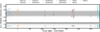 |
Fig. 3 Top panel: radial velocity time series (coloured dots) and best-fit Keplerian model (grey line) for the juliet fit of the WASP-121 public RVs. The fitted instrumental offsets μinstrument have been subtracted from each time series. Bottom panel: residuals of the fit. |
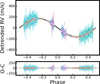 |
Fig. 4 Top panel: phase-folded RVs (coloured dots) and best-fit Keplerian model (black line). The colours of the RV points match those in Fig. 3. Both the fitted instrumental offsets and the GP components (where applicable) have been subtracted from each time series. Bottom panel: residuals of the fit. |
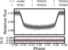 |
Fig. 5 Top panel: stacked phase-folded TESS photometry (grey dots), binned data for each sector (coloured dots), and best-fit model (black line) for the juliet fit of the WASP-121 TESS photometry. Bottom panel: residuals of the fit. |
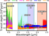 |
Fig. 6 Atmospheric models (transit depth as function of wavelength) for OH (brown), Fe (green), V (magenta), CO (red), H2O (blue), and TiO (orange) generated with the SCARLET code. The shaded regions highlight the spectral coverage of each instrument. The range of the wavelength of HARPS is in yellow, the NIRPS region is in cyan, and the CRIRES+ H-band and K-band are in purple and orange, respectively. |
WASP-121b SCARLET atmospheric posteriors from the retrieval analysis on the HARPS, NIRPS, and CRIRES+ time series combined.
4.2 Atmospheric retrieval recipe
We performed a retrieval analysis to constrain a range of key atmospheric parameters, as summarised in Table 5. These include the volume mixing ratios (VMRs) of several atomic and molecular species - specifically, log10 H2O, log10 CO, log10 OH, log10Fe, log10V, and log10H−. The VMR of a species, X, is defined as the logarithm (base 10) of its volume mixing ratio:
 (2)
(2)
In addition, we retrieved the electron density (log10 e−), atmospheric temperature (T), orbital velocity semi-amplitude of the planet (Kp), systemic velocity (Vsys), and the rotational broadening full width at half maximum (FWHM). To infer the posterior probability distributions, we used a high-resolution retrieval prescription (Brogi & Line 2019; Gibson et al. 2020, 2022) that utilises SCARLET to generate the transmission spectra as detailed in Pelletier et al. (2021, 2023, 2024); Bazinet et al. (2024); Vaulato et al. (2025). The Bayesian framework uses the likelihood approach from Gibson et al. (2020) and the emcee code as a sampler (Foreman-Mackey et al. 2013). We ran the atmospheric retrieval on the HARPS, NIRPS and CRIRES+ transits simultaneously. We also included the TESS photometric point from Bourrier et al. (2020) to ensure all sampled models match the true planetary radius. We opted for an atmospheric ‘free’ retrieval approach, allowing abundances of individual species to be fitted independently as free parameters, rather than enforcing any assumptions about the atmospheric chemistry (e.g., equilibrium chemistry). The free retrieval assumes input priors on the abundance profiles to be well-mixed (constant with altitude and hence uniform in pressure). We assumed a uniform prior distribution, U(−12,0), for all absolute abundance. Assuming the high temperature of WASP-121b prevents the formation of optically thick clouds, the continuum level is set by the H− continuum, which is parametrised with the abundances of H− and e−. We set up the free retrieval to fit for abundances of H2O and OH as representative of thermal dissociation processes, according to the following chemical reactions (Parmentier et al. 2018):

Moreover, we retrieved the abundance of CO as the main carbon-bearing species in ultra-hot Jupiters atmosphere, TiO acting as primary opacity source in optical wavelength, and the abundance of refractory species detected via cross-correlation (e.g. Fe and V). We let the retrieval free to fit for the abundance of H− and the electron density, used to infer the continuum opacity given by H−bound-free and free-free absorption transitions (Arcangeli et al. 2018; Parmentier et al. 2018; Vaulato et al. 2025).
Other than abundance parameters, the retrieval fits for the atmospheric temperature, the orbital velocities Kp and Vsys, and a Gaussian rotational broadening parameter in order to account for the observed signal appearing more ‘blurred’ in the Kp-Vsys space than what would be expected from the instrumental resolution alone. We assumed that an isothermal profile is likely a valid approximation for the average thermal structure probed in transmission, based on Gandhi et al. (2023) (see their Figure 11) and Maguire et al. (2023) (see their Figure 3, retrieved temperature-pressure profile).
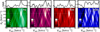 |
Fig. 7 Detections of CCFs for Fe (SNR=5.8), CO (SNR=5.0), and V (SNR=4.7), and non-detection of H2O (SNR<2.0) in the transmission spectrum of WASP-121b. Each squared panel shows the two-dimensional cross-correlation map in the velocity-velocity space (Kp − Vsys). The white dashed lines indicate the expected position of the planetary signal within the velocity-velocity space, namely the expected orbital (~216 km s−1, Hoeijmakers et al. 2024) and systemic (3 8.35 ± 0.02 km s−1, Delrez et al. 2016) velocities of WASP-121b. The rectangular panels on top depicts the one-dimensional cross-correlation of each species as signal-to-noise ratio versus systemic velocity. Detections of Fe and V are primarily driven by the optical HARPS observations, while the CO detection by the infrared CRIRES+ data (mostly K-band observations). |
5 Results
5.1 Detections of cross-correlation functions
We detected the signatures of Fe (SNR=5.8) and V (SNR=4.7) by combining HARPS optical spectra, and CO (SNR=5.0) from CRIRES+ spectra in the K-band (Figure 7). We thus confirm previous results reported in Section 1. Neither NIRPS nor CRIRES+ H-band spectra yield a statistically significant H2O signal (SNR<2.0) in the Kp-Vsys space (see H2O map in Figure 7). However, the latter datasets contribute at constraining H−, OH, and H2O individual abundances in the retrieval analysis, as discussed in Sect. 5.2. The non-detection of refractory elements (Fe or Ti) in the NIRPS range could be due to the fewer and weaker spectral lines exhibited by these species compared to those in the optical range of HARPS (Figure 6). However, Vaulato et al. (2025) showed that in the case of NIRPS observations of the ultrahot gas giant WASP-189b, these lines are damped below -1.6 μm by the H− bound-free continuum (Arcangeli et al. 2018; Parmentier et al. 2018, see also Fig. 7 in Lothringer et al. 2018).
The SNR maxima of the one-dimensional cross-correlation functions of all three detected signals (top panel in Fig. 7) are slightly offset (< 10 km s−1, more specifically the signal peaks between 31-36 km s−1) with respect to the reference Vsys ~ 38.35 km s−1 (Delrez et al. 2016). This could indicate the presence of winds at sub-millibar pressures (see Sect. 5.3). The consistent blueshifted signals observed for the refractory elements (e.g. Fe and V) are in agreement with sub-to-antistellar circulation in atmospheric layers, as reported by Seidel et al. (2025) (see their Figure 2). Alternatively, systematic offsets (different instrument by instrument) or instrumental noise might be responsible for the observed blueshifted features, hence the offset might have a non-physical meaning (not related to atmospheric circulations). However, it is worth noticing that the blueshift is fairly consistent between the HARPS-driven Fe and V detections, and the CRIRES+-driven CO detection, further supporting the hypothesis of day-to-night winds.
5.2 Retrieval results
We summarise the key results of the free atmospheric retrieval analysis on WASP-121b HARPS, NIRPS, and CRIRES+ time series combined in Figures 8, 9, and Table 5. We retrieved the best-fit abundances for the chemical species injected in our model (i.e. Fe, V, CO, H2O, OH, TiO, H−, and e−). However, retrieved absolute abundances are not informative of the underlying chemistry in a planet’s atmosphere, as they significantly rely on model assumptions and, thus, are model dependent. Furthermore, retrieved absolute abundances rely on abundance constraints that are generally broad, with uncertainties of the order of 1 dex, and dependent on prior distributions (Gibson et al. 2022, see also Burningham et al. 2017). Namely, the spectra can be well-fitted by models with different parameters (e.g. reference pressure, continuum level, or planet radius).
Inferring the volume mixing ratios of one specific absorbing gas of the atmosphere by directly measuring its absorption features is challenging because it depends on different combinations of the planet’s radius and the mixing ratio assumed, yielding the same number density. For instance, two atmospheres with different absorber mixing ratios might have consistent pressure and densities leading to similar absorption spectral features (Benneke & Seager 2012, see their Figure 4 and Section 4.1.1). Thus, this leads to strong correlations indicating that relative abundances of species are constrained more accurately than absolute abundances (Gibson et al. 2022, see their Section 5).
To investigate the chemical composition of WASP-121b’s atmosphere, we calculated abundance ratios between pairs of species, X and Y, using their volume mixing ratios as defined in Equation (2). The abundance ratio is expressed in logarithmic form as
 (3)
(3)
We constrained the relative abundances for  ,
,  ,
,  and
and  (Table 5, Figure 8). We then compared the retrieved abundance ratios with predictions from modelled equilibrium chemistry (Kitzmann et al. 2024). Overall, the retrieved abundance ratios are consistent with a 1 × solar metallicity and a solar C/O ratio ((C/O)⊙ = 0.59 ± 0.08; Asplund et al. 2021).
The fraction of H2O relative to CO (Figure 8, second panel) is 1 dex underabundant (sub-solar) than predictions from FastChem (but still consistent with solar within 1-σ), likely due to water being partially dissociated into OH and O (Parmentier et al. 2018) at the high temperatures at play. This underabundance would be even more pronounced if assuming the stellar C/O rather than the solar C/O. We, indeed, retrieve a temperature  , assumed to be uniform across the atmosphere at the pressures probed, in agreement with Gandhi et al. (2023). At this temperature, the abundance of CO for a nearly-solar C/O remains unchanged. Therefore, according to Madhusudhan (2012), the log(H2O/CO) ratio is expected to be close to unity for a nearly solar C/O ratio, in agreement with our retrieved abundance ratio (
 ).
).
Intriguingly, the free retrieval constrains the abundance of H2O despite the lack of a cross-correlation detection in our data (Figure 7, forth panel). This constraint is rather driven by the retrieval preferring to add water. In fact, H2O has been detected in both high- and low-resolution observations (Evans et al. 2016; Wardenier et al. 2024). Therefore, a non-detection in the crosscorrelation space is more likely due to the limited sensitivity of our data rather than the absence of H2O in WASP-121b atmosphere. Notably, Wardenier et al. (2024) reported a significant H2O detection only after stacking three transits gathered with IGRINS installed on Gemini, a 8-m class telescope. The breaking up of water molecules is significant in ultra-hot gas giants, where it must be accounted for when inferring chemical abundances, especially in comparison to more thermally stable species such as CO. Carbon monoxide is, indeed, a benchmark molecule to compare with (Parmentier et al. 2018; Savel et al. 2023). The reason is twofold: (i) due to its chemical robustness (thanks to the triple covalent bond), CO is less prone to thermal dissociation (via CO ⇄ C + O), thus remaining nearly constant with pressure (with the exception of known torrid exoplanets with fully dissociated atmospheres, such as KELT-9b, Gaudi et al. 2017; Hoeijmakers et al. 2018); and, (ii) CO is also poorly sensitive to model assumptions on its abundance profile, being resistant to thermal dissociation. The log(H2O/CO) abundance ratio also serves as an indicator of the atmospheric region probed by our data, as well as of the dissociation and condensation of volatile compounds. Indeed, water condensates and dissociates more readily than CO for the reasons illustrated above. According to the retrieved quantity, which relies on model assumptions, and the chemistry predictions, we sample the pressure layer from sub-to-millibar (~10−4−10−3 bar), hence, we do not have access to the inflated upper atmosphere of WASP-121b, but rather we have insights to lower pressures.
We find that the retrieved log(CO/Fe) ratio is consistent with the solar value (Figure 8, third panel), implying that the planet’s atmosphere likely experiences a moderate-to-high temperature that is not extreme enough to dissociate CO molecules and not cool enough to allow extensive Fe rainout. The log(CO/Fe) ratio can be also interpreted as a proxy of the volatile-to-refractory budget, i.e. the ice-to-rock ratio. Moreover, the log(CO/Fe) ratio, being consistent with a model assuming a solar amount of carbon relative to oxygen, suggests that the atmosphere is not heavily skewed towards either a super-solar abundance of carbon or oxygen, but is instead chemically balanced. However, an atmosphere carrying a C/O ratio consistent-with-solar, likely favour a surplus of oxygen which is mostly bound in water molecules at low temperatures but which is set free by thermal dissociation of H2O at high temperatures (as the case of ultrahot gas giants) and pairs to form CO (CH4+H2O ⇄ CO+3H2) and OH (H2O ⇄ 2H+O) (Madhusudhan 2012).
The retrieved consistency with a C/O=solar contrasts with: (i) the carbon-enriched (volatile-enriched relative to refractory) atmosphere reported by Pelletier et al. (2024), which shows a super-solar C/O ratio (C/O =  ) from a free retrieval and a super-stellar ratio (C/O =
  ) from a chemically consistent retrieval; and (ii) the super-stellar C/O ratio (C/O =
  ) and a moderately super-stellar refractory-to-volatileratio (
 × stellar) found by Smith et al. (2024) under chemical equilibrium conditions. Despite both studies report elevated C/O ratios from dayside observations, Pelletier et al. (2024) favour a scenario enriched in ice-forming elements over rock-forming elements, suggesting the planet formed farther out in the disc beyond the ice-line, while Smith et al. (2024) suggest that WASP-121b likely formed between the soot line and the H2O snow line (Lothringer et al. 2021; Chachan et al. 2023). Our finding places WASP-121b in the nearly chemically balanced regime, not markedly favouring either a volatile rich or refractory-rich formation environment. However, it is worth noticing that our results based on transit time series rather than dayside observations, thus our data probe a different altitude in the atmosphere of WASP-121b.
We retrieve a log(V/Fe) ratio that is consistent with chemical models assuming a solar composition (Figure 8, forth panel) indicating that the refractory balance is preserved in the atmosphere of WASP-121b, fully in agreement with equilibrium chemistry predictions. Our retrieved elemental ratio is also well consistent with that of Maguire et al. (2023) (see their Figure 4, second panel), based on three transits observed with ESPRESSO/VLT and fully in agreement with one UVES transit used as a benchmark.
The measured log(H−/Fe) ratio (Figure 8, first panel) can be a tracer of both the opacity contribution from H− in the (near-) infrared regime, and the ionisation processes involving the electron density associated with the ionisation of metals, which are the primary source of free electrons (Bell & Berrington 1987; John 1988).
The retrieval fails to constrain the abundance of free electrons (Figure 9), likely due to either the spectral range of our observations does not extend to wavelengths sensitive to the free-free transitions to form H , or the inefficiency of metal ionisation within the pressure and temperature regime probed by the data. H bound-free absorption can dominate the spectrum below ~1.6 μm, masking spectral features from species such as H2O and TiO. Similarly, the retrieval sets an upper limit for TiO, despite also non-detected in cross-correlation. Nevertheless, caution is warranted, as the line list used for TiO may lack the accuracy required to draw firm conclusions about the presence of TiO in the atmosphere of WASP-121b (Prinoth et al. 2025). However, Prinoth et al. (2025) reported a significant detection of Ti (albeit at a weaker strength then expected) in high signal-to-noise optical transits, suggesting that TiO may also be present.
In ultra-hot gas giants, ionisation involves both thermal processes and photoionisation (Kitzmann et al. 2018; Fossati et al. 2020). However, the effects of the latter is not considered in the equilibrium chemistry models. Hence, the modelled log(H−/Fe) profile primarily reflects thermally driven ionisation processes occurring in WASP-121b at (sub-)millibar pressures. In this context, the measured log(H−/Fe) is consistent with FastChem models of a solar composition, and function as a thermometer in thermal equilibrium atmospheres according to the Saha ionisation equation (Saha 1920). Even though the retrieved elemental hydride-to-Fe ratio is consistent with model predictions within 1σ, the median of the Gaussian distribution peaks at marginally super-solar values, hinting at either an elevated abundance of hydride continuum opacity similar to what found in WASP-189b (Vaulato et al. 2025) but likely to compensate for missing opacity contributions in the model assumption, or a depleted Fe content due to condensation. The atmosphere of WASP-121b boasts a wealth of detected chemical species (see Section 1 for a complete literature overview) which we decided not to include in our atmospheric retrieval calculation and model. The main reason behind our choice is computational limitations.
Therefore, H− is supposedly overcompensating for other missing opacity sources from species not included in our model. Indeed, the continuum should be handled mainly by the hydride and so by the density of free-electrons (e-), which have proven to be the principal continuum absorbers, particularly in ultra-hot gas giants (Parmentier et al. 2018; Arcangeli et al. 2018; Vaulato et al. 2025). We also surmise that photoionisation mechanisms might become relevant since the log(H− /Fe) ratio peaks at about 10−4, higher than predicted by solar chemical equilibrium models (10−5). Nevertheless, the retrieved log(H−/Fe) abundance ratio results consistent with solar models within 1 dex.
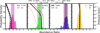 |
Fig. 8 Key retrieved results. The four distributions represent the probability density of retrieved chemical abundance ratios (in logarithmic scale). Overplotted the FastChem model predictions in chemical equilibrium as varying the metallicity and the C/O ratio. FastChem theoretical models are displayed as function of the pressure in bar. |
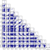 |
Fig. 9 Retrieved constraints on the atmospheric and orbital properties from HARPS, NIRPS and CRIRES+ combined transits of WASP-121b. We assumed a free atmospheric retrieval condition and hence a well-mixed chemistry (constant with altitude). |
5.3 Orbital velocities
We retrieved a systemic velocity of  . We also constrained an orbital velocity of
  .
.
Leveraging the largest RV dataset of WASP-121b to date, we update the orbital parameters, deriving the orbital velocity Kp from the stellar reflex motion obtained via the juliet fitting routine, as detailed in Section 3. By comparing our derived orbital velocities from both the RV analysis and the atmospheric retrieval routine, we calculate the velocity offset, ΔKp3 (Wardenier et al. 2025), which reflects the rate of change of the Doppler shift of the planetary signal across the orbital phases from (0,0) km s−1 in the planet rest frame. By inspecting the Kp - Vsys maps, the planetary signal appears overall diffused (not a point-like source), likely due to dynamics and 3D effects, which are modelled as one free rotational broadening parameter in the atmospheric retrieval and retrieved to be  km s−1, consistent with the expectations. Transmission data are generally more sensitive to atmospheric dynamics, hence, we could expect a rotational broadening parameter that slightly differs from the planet rotation rate4 The retrieved rotational broadening parameter is not significantly under or over-broadened, thus ruling out potential resolution biases. In case of Fe, V and CO, the signal-to-noise ratio peaks at both lower Kp and lower Vsys values (see Figure 7) than the reference ones, resulting in blueshifted signals along the RV axis and a change in slope (i.e. acceleration) along the orbital velocity axis. These results can be contextualised within the framework proposed by Wardenier et al. (2023, 2024) who present detailed three-dimensional global circulation models for WASP-121b, and simulate the resulting high-resolution transmission spectra across different dynamical regimes. We consider four GCMs (see Figure 10): the first is a drag-free (τdrag → ∞) model illustrated in Parmentier et al. (2018), while the other three models are presented in Tan et al. (2024) including one drag-free (τdrag → ∞) model, one weak-drag model (τdrag = 106 s), and one with a strong-drag prediction (τdrag = 104 s), where τ is the uniform drag timescale. The dragtimescale variable represents the time needed for a parcel of air to lose a substantial percentage of its kinetic energy. It describes the wind speed, thus the efficiency of heat redistribution, and the Doppler shifts observed in the spectra. The zero-drag model accounts for a super-rotating equatorial jet (Wardenier et al. 2021), while jet formation is suppressed in the drag-models. Indeed, in both weak- and strong-drag models, the wind profile is mainly dominated by day-to-night flows. Moreover, the day-tonight contrast is preserved in all models being the planet tidally locked. Therefore, these global circulation models demonstrate that the presence, or absence, of atmospheric drag strongly modulates the Doppler shift of the planetary signal. In particular, drag-free models naturally produce a symmetric latitudinal temperature structure and high longitudinal temperature gradients at the terminator (strong day-to-night temperature variations), resulting in measurable Doppler shifts in the planetary trail due to winds and rotation. Indeed, the changing and evolving structure of the planet’s atmosphere as viewed at different phases results in a variation of the position of the planet’s spectral lines, eventually resulting in a measurable shift in the Kp . This is consistent with our detection of a negative ΔKp and ΔVsys for Fe, V and CO. Indeed, GCMs predict a decrease in the observed Kp, specifically producing a negative ΔKp, regardless of the drag.
However, as highlighted in Table 6 and Figure 10, the calculation of ΔKp is sensitive to the assumed stellar mass, which feeds directly into the derived orbital velocity. Differences in M⋆ lead to non-negligible changes in the interpretation of the Doppler shift and, therefore, in how well our observations align with specific GCM predictions. This emphasises the importance of using consistent stellar parameters when comparing observationally derived kinematic shifts to model outputs.
WASP-121 is known as a hot, F6-type star, with a moderate chromospheric stellar activity level (logR′HK ≃ −4.8 measured by Borsa et al. 2021). Bourrier et al. (2020) also reported on magnetically active regions at the surface of WASP-121, visible in the periodogram of the RV residuals (see their Figure 3). Moreover, the moderate-to-fast rotation of WASP-121 (v sin(i) = 11.90 ± 0.31 km s−1, Borsa et al. 2021) broadens the few stellar spectral lines typical of A- and F-type stars, blending lines that are usually isolated and more ‘peaky’ in cold and slow rotating stars. As a result, deriving the chemical composition of these stars (e.g. the metallicity) becomes challenging and thus extracting stellar parameters such as the stellar mass is more difficult. Figure 10 clearly illustrates the variation in the computed ΔKp as function of the stellar mass, but using the stellar reflex motion obtained from the RV fitting in all four scenarios presented. Vertical lines mark the ΔKp values predicted by GCMs. We can surely claim that all computed planet’s orbital velocity are consistent with either weak-drag or drag-free models, while the strong-drag configuration is ruled out, regardless of the model. These results are fully consistent with Wardenier et al. (2024).
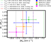 |
Fig. 10 Vecolity offset, ΔKp, as a function of different stellar masses. This plot serves to visualise the Table 6 in comparison with global circulation model predictions. Each data point with uncertainties corresponds to the computed ΔKp as a function of the stellar mass (reported in Table 6) as derived by Delrez et al. (2016) (M⋆ = 1.35 ± 0.08 M⊙), Borsa et al. (2021) (M⋆ = 1.38 ± 0.02 M⊙), Sing et al. (2024) (M⋆ = 1.33 ± 0.02 M⊙), and Prinoth et al. (2025) (M⋆ = 1.42 ± 0.03 M⊙), respectively. Uncertainties are calculated via error propagation. Vertical lines mark the GCM predictions, namely models with zero, weak, and strong drag by Tan et al. (2024) and drag-free models by Parmentier et al. (2018). |
Mass reference. We computed ΔKp assuming different stellar masses by keeping the stellar reflex motion fixed.
6 Conclusions
In this work, we have presented an atmospheric retrieval analysis of the ultra-hot Jupiter WASP-121b by combining highresolution transmission spectra from HARPS, NIRPS, and CRIRES+ (in both the K and H photometric bands). Leveraging the large high-resolution dataset, we constrained the planet’s atmospheric composition and orbital dynamics through a free retrieval approach using the SCARLET code.
We have reported the retrieved relative chemical abundances of key species, including Fe, V, CO, H2O, OH, TiO, H−, and e−. While absolute abundances remain highly model dependent and less informative, abundance ratios offer a more robust window into the atmospheric processes and underlying chemistry. Our results indicate that the atmosphere of WASP-121b is broadly consistent with a solar metallicity and a solar C/O ratio. This suggests that chemical equilibrium remains largely preserved at the pressure levels probed (~10−4−10−3 bar), with no strong evidence for substantial alteration from disequilibrium processes such as rainout, photochemistry, or deep vertical mixing.
Notably, we constrain the log(H2O/CO) ratio to be 1 dex sub-solar compared to chemical equilibrium predictions from FastChem, a result consistent with partial water dissociation at high temperatures. Despite lacking of a direct cross-correlation detection of H2O, the retrieval favours the inclusion of water vapour to reproduce the observed spectra. The retrieved temperature of  K reinforces the expectation of thermal dissociation affecting volatile species, such as water.
The log(CO/Fe) and log(V/Fe) ratios are in agreement with solar values, indicating that refractory-to-volatile balances are maintained and that CO remains stable against dissociation, which is consistent with its high bond energy. These findings reinforce the utility of CO as a chemically robust reference molecule in high-temperature atmospheres. In contrast, log(H− /Fe) emerges as a potentially sensitive tracer of thermal ionisation. The retrieval returns a value 1 dex elevated (but still within 1σ) compared to solar predictions, hinting at an elevated abundance of hydride continuum opacity but likely to compensate for missing opacity contributions in the model assumption, or at a depleted Fe content due to condensation. The retrieval fails to constrain the electron density, limiting our ability to distinguish between enhanced H− opacity and Fe depletion through condensation.
Intriguingly, the cross-correlation signals for Fe, V, and CO appear blueshifted along the RV axis and peak at a lower orbital velocity than compared to the reference one in the Kp-Vsys space, suggesting the presence of equatorial winds and rotational broadening. These results are potentially indicative of drag-free or weak-drag atmospheric circulation as predicted by global circulation models. These models support a scenario in which CO probes higher-altitude layers subject to faster wind speeds, while Fe and V trace deeper regions where rotation dominates.
We also re-examined the planet’s orbital parameters using the largest RV dataset to date. We report on a global fit to RV measurements (from CORALIE, HARPS, NIRPS, and ESPRESSO observations) and photometric light curves from TESS in order to refine the planetary orbital parameters. Indeed, thanks to the broad RV dataset, the orbital parameters of the system are improved. By comparing the derived orbital velocity from both the RV analysis and the atmospheric retrieval, we estimated the velocity offset, ΔKp, and find it is non-zero, but also consistent with predictions from either drag-free or weak-drag 3D global circulation models while cautioning the non-negligible dependence on the stellar mass assumed.
Overall, our results provide a chemically and dynamically coherent picture of WASP-121b's atmosphere. The planet’s bulk composition appears largely unaltered by disequilibrium processes, while local deviations - such as water dissociation and thermal ionisation - highlight the complexity of atmospheric processes in ultra-hot environments. This study demonstrates the power of combining high-resolution multi-instrument datasets with retrieval techniques to simultaneously probe chemical composition and atmospheric dynamics.
Future work will benefit from improved opacity databases - especially for TiO - and more physically complete models incorporating vertical mixing, photochemistry, and cloud condensation. The integration of low- and high-resolution datasets within a joint retrieval framework will be essential to further refining molecular abundance constraints.
Acknowledgements
This work has been carried out within the framework of the NCCR PlanetS supported by the Swiss National Science Foundation under grants 51NF40_182901 and 51NF40_205606. RA acknowledges the Swiss National Science Foundation (SNSF) support under the Post-Doc Mobility grant P500PT_222212 and the support of the Institut Trottier de Recherche sur les Exoplanètes (IREx). RA, JPW, ÉA, FBa, BB, NJC, RD, LMa & CC acknowledge the financial support of the FRQ-NT through the Centre de recherche en astrophysique du Québec as well as the support from the Trottier Family Foundation and the Trottier Institute for Research on Exoplanets. ML, HC & BA acknowledge support of the Swiss National Science Foundation under grant number PCEFP2_194576. DE and MS acknowledge support from the Swiss National Science Foundation for project 200021_200726. VV, SP, DE, &MS acknowledge the financial support of the SNSF. NN, JIGH, RR, ASM & AKS acknowledge financial support from the Spanish Ministry of Science, Innovation and Universities (MICIU) projects PID2020-117493GB-I00 and PID2023-149982NB-I00. NN acknowledges financial support by Light Bridges S.L, Las Palmas de Gran Canaria. NN acknowledges funding from Light Bridges for the Doctoral Thesis "Habitable Earth-like planets with ESPRESSO and NIRPS", in cooperation with the Instituto de Astrofísica de Canarias, and the use of Indefeasible Computer Rights (ICR) being commissioned at the ASTRO POC project in the Island of Tenerife, Canary Islands (Spain). The ICR-ASTRONOMY used for his research was provided by Light Bridges in cooperation with Hewlett Packard Enterprise (HPE). XDu acknowledges the support from the European Research Council (ERC) under the European Union’s Horizon 2020 research and innovation programme (grant agreement SCORE No. 851555) and from the Swiss National Science Foundation under the grant SPECTRE (No 200021_215200). This work was supported by grants from eSSENCE (grant number eSSENCE@LU 9:3), the Swedish National Research Council (project number 2023 05307), The Crafoord foundation and the Royal Physiographic Society of Lund, through The Fund of the Walter Gyllenberg Foundation. ÉA, FBa, RD & LMa acknowledges support from Canada Foundation for Innovation (CFI) program, the Université de Montréal and Université Laval, the Canada Economic Development (CED) program and the Ministere of Economy, Innovation and Energy (MEIE). SCB, ED-M, NCS & ARCS acknowledge the support from FCT - Fundaçåo para a Ciên-cia e a Tecnologia through national funds by these grants: UIDB/04434/2020, UIDP/04434/2020. SCB acknowledges the support from Fundaçåo para a Ciên-cia e Tecnologia (FCT) in the form of a work contract through the Scientific Employment Incentive program with reference 2023.06687.CEECIND and DOI 10.54499/2023.06687.CEECIND/CP2839/CT0002. XB, XDe and TF acknowledge funding from the French ANR under contract number ANR24-CE493397 (ORVET), and the French National Research Agency in the framework of the Investissements d’Avenir program (ANR-15-IDEX-02), through the funding of the “Origin of Life” project of the Grenoble-Alpes University. The Board of Observational and Instrumental Astronomy (NAOS) at the Federal University of Rio Grande do Norte’s research activities are supported by continuous grants from the Brazilian funding agency CNPq. This study was partially funded by the Coordenaçåo de Aperfeiçoamento de Pessoal de Nível Superior - Brasil (CAPES) - Finance Code 001 and the CAPES-Print program. BLCM acknowledge CAPES postdoctoral fellowships. BLCM acknowledges CNPq research fellowships (Grant No. 305804/2022-7). NBC acknowledges support from an NSERC Discovery Grant, a Canada Research Chair, and an Arthur B. McDonald Fellowship, and thanks the Trottier Space Institute for its financial support and dynamic intellectual environment. JRM acknowledges CNPq research fellowships (Grant No. 308928/2019-9). ED-M further acknowledges the support from FCT through Stimulus FCT contract 2021.01294.CEECIND. ED-M acknowledges the support by the Ramón y Cajal contract RyC2022-035854-I funded by MICIU/AEI/10.13039/501100011033 and by ESF+. ICL acknowledges CNPq research fellowships (Grant No. 313103/2022-4). CMo acknowledges the funding from the Swiss National Science Foundation under grant 200021_204847 “PlanetsInTime”. Co-funded by the European Union (ERC, FIERCE, 101052347). Views and opinions expressed are however those of the author(s) only and do not necessarily reflect those of the European Union or the European Research Council. Neither the European Union nor the granting authority can be held responsible for them. GAW is supported by a Discovery Grant from the Natural Sciences and Engineering Research Council (NSERC) of Canada.
KAM acknowledges support from the Swiss National Science Foundation (SNSF) under the Postdoc Mobility grant P500PT_230225. ARCS acknowledges the support from Fundaçao para a Ciência e a Tecnologia (FCT) through the fellowship 2021.07856.BD. BP acknowledges financial support from the Walter Gyllenberg Foundation. AKS acknowledges financial support from La Caixa Foundation (ID 100010434) under the grant LCF/BQ/DI23/11990071. BT acknowledges the financial support from the Wenner-Gren Foundation (WGF2022-0041). AP acknowledges support from the Unidad de Excelencia María de Maeztu CEX2020-001058-M programme and from the Generalitat de Catalunya/CERCA.
References
- Anderson, D. R., Temple, L. Y., Nielsen, L. D., et al. 2018, arXiv e-prints [arXiv:1809.04897] [Google Scholar]
- Arcangeli, J., Désert, J.-M., Line, M. R., et al. 2018, ApJ, 855, L30 [Google Scholar]
- Arcangeli, J., Désert, J.-M., Parmentier, V., et al. 2019, A&A, 625, A136 [NASA ADS] [CrossRef] [EDP Sciences] [Google Scholar]
- Asplund, M., Amarsi, A. M., & Grevesse, N. 2021, A&A, 653, A141 [NASA ADS] [CrossRef] [EDP Sciences] [Google Scholar]
- Bazinet, L., Pelletier, S., Benneke, B., Salinas, R., & Mace, G. N. 2024, AJ, 167, 206 [NASA ADS] [CrossRef] [Google Scholar]
- Bazinet, L., Allart, R., Benneke, B., et al. 2025, A&A, 701, A276 [NASA ADS] [CrossRef] [EDP Sciences] [Google Scholar]
- Bell, K. L., & Berrington, K. A. 1987, J. Phys. B: At. Mol. Phys., 20, 801 [NASA ADS] [CrossRef] [Google Scholar]
- Bell, T. J., & Cowan, N. B. 2018, ApJ, 857, L20 [Google Scholar]
- Benneke, B. 2015, arXiv e-prints [arXiv:1504.07655] [Google Scholar]
- Benneke, B., & Seager, S. 2012, ApJ, 753, 100 [NASA ADS] [CrossRef] [Google Scholar]
- Benneke, B., & Seager, S. 2013, ApJ, 778, 153 [Google Scholar]
- Benneke, B., Cowan, N., Rowe, J., et al. 2019, https://doi.org/10.5281/zenodo.3827830 [Google Scholar]
- Birkby, J. L., Kok, D., J, R., et al. 2013, MNRAS, 436, L35 [NASA ADS] [CrossRef] [Google Scholar]
- Borsa, F., Allart, R., Casasayas-Barris, N., et al. 2021, A&A, 645, A24 [EDP Sciences] [Google Scholar]
- Borysow, A. 2002, A&A, 390, 779 [NASA ADS] [CrossRef] [EDP Sciences] [Google Scholar]
- Bouchy, F., Doyon, R., Pepe, F., et al. 2025, A&A, 700, A10 [NASA ADS] [CrossRef] [EDP Sciences] [Google Scholar]
- Bourrier, V., Ehrenreich, D., Lendl, M., et al. 2020, A&A, 635, A205 [NASA ADS] [CrossRef] [EDP Sciences] [Google Scholar]
- Broeg, C., Fernández, M., & Neuhäuser, R. 2005, Astron. Nachr., 326, 134 [NASA ADS] [CrossRef] [Google Scholar]
- Brogi, M., & Line, M. R. 2019, AJ, 157, 114 [Google Scholar]
- Brogi, M., Snellen, I. A. G., de Kok, R. J., et al. 2012, Nature, 486, 502 [Google Scholar]
- Burningham, B., Marley, M. S., Line, M. R., et al. 2017, MNRAS, 470, 1177 [NASA ADS] [CrossRef] [Google Scholar]
- Casasayas-Barris, N., Borsa, F., Palle, E., et al. 2022, A&A, 664, A121 [NASA ADS] [CrossRef] [EDP Sciences] [Google Scholar]
- Chachan, Y., Knutson, H. A., Lothringer, J., & Blake, G. A. 2023, ApJ, 943, 112 [NASA ADS] [CrossRef] [Google Scholar]
- Chakraborty, H., Lendl, M., Akinsanmi, B., Petit dit de la Roche, D. J. M., & Deline, A. 2024, A&A, 685, A173 [NASA ADS] [CrossRef] [EDP Sciences] [Google Scholar]
- Collier Cameron, A., Guenther, E., Smalley, B., et al. 2010, MNRAS, 407, 507 [NASA ADS] [CrossRef] [Google Scholar]
- Cutri, R. M., Skrutskie, M. F., van Dyk, S., et al. 2003, VizieR Online Data Catalog: 2MASS All-Sky Catalog of Point Sources (Cutri+ 2003), VizieR On-line Data Catalog: II/246. Originally published in: University of Massachusetts and Infrared Processing and Analysis Center, (IPAC/California Institute of Technology) (2003) [Google Scholar]
- Dekker, H., D’Odorico, S., Kaufer, A., Delabre, B., & Kotzlowski, H. 2000, SPIE Conf. Ser., 4008, 534 [Google Scholar]
- Delrez, L., Santerne, A., Almenara, J.-M., et al. 2016, MNRAS, 458, 4025 [NASA ADS] [CrossRef] [Google Scholar]
- Dorn, R. J., Bristow, P., Smoker, J. V., et al. 2023, A&A, 671, A24 [NASA ADS] [CrossRef] [EDP Sciences] [Google Scholar]
- Ehrenreich, D., Lovis, C., Allart, R., et al. 2020, Nature, 580, 597 [Google Scholar]
- Espinoza, N., Kossakowski, D., & Brahm, R. 2019, MNRAS, 490, 2262 [Google Scholar]
- Evans, T. M., Sing, D. K., Wakeford, H. R., et al. 2016, ApJ, 822, L4 [NASA ADS] [CrossRef] [Google Scholar]
- Evans-Soma, T M., Sing, D. K., Barstow, J. K., et al. 2025, Nat. Astron. [arXiv:2506.01771] [Google Scholar]
- Follert, R., Dorn, R. J., Oliva, E., et al. 2014, in Ground-based and Airborne Instrumentation for Astronomy V, 9147 (International Society for Optics and Photonics), 914719 [Google Scholar]
- Foreman-Mackey, D., Hogg, D. W., Lang, D., & Goodman, J. 2013, PASP, 125, 306 [Google Scholar]
- Foreman-Mackey, D., Agol, E., Ambikasaran, S., & Angus, R. 2017, AJ, 154, 220 [Google Scholar]
- Fossati, L., Shulyak, D., Sreejith, A. G., et al. 2020, A&A, 643, A131 [NASA ADS] [CrossRef] [EDP Sciences] [Google Scholar]
- Fulton, B. J., Petigura, E. A., Blunt, S., & Sinukoff, E. 2018, PASP, 130, 044504 [Google Scholar]
- Gandhi, S., Kesseli, A., Zhang, Y., et al. 2023, AJ, 165, 242 [NASA ADS] [CrossRef] [Google Scholar]
- Gapp, C., Evans-Soma, T M., Barstow, J. K., et al. 2025, AJ, 169, 341 [Google Scholar]
- Garcia, L. J., Timmermans, M., Pozuelos, F. J., et al. 2022, MNRAS, 509, 4817 [Google Scholar]
- Gaudi, B. S., Stassun, K. G., Collins, K. A., et al. 2017, Nature, 546, 514 [NASA ADS] [Google Scholar]
- Gibson, N. P., Merritt, S., Nugroho, S. K., et al. 2020, MNRAS, 493, 2215 [Google Scholar]
- Gibson, N. P., Nugroho, S. K., Lothringer, J., Maguire, C., & Sing, D. K. 2022, MNRAS, 512, 4618 [NASA ADS] [CrossRef] [Google Scholar]
- Gray, D. F. 2021, The Observation and Analysis of Stellar Photospheres, 4th edn. (Cambridge: Cambridge University Press) [Google Scholar]
- Grimm, S. L., & Heng, K. 2015, ApJ, 808, 182 [NASA ADS] [CrossRef] [Google Scholar]
- Grimm, S. L., Malik, M., Kitzmann, D., et al. 2021, ApJSS, 253, 30 [Google Scholar]
- Hellier, C., Anderson, D. R., Cameron, A. C., et al. 2009, Nature, 460, 1098 [NASA ADS] [CrossRef] [Google Scholar]
- Helling, C., Lewis, D., Samra, D., et al. 2021, A&A, 649, A44 [NASA ADS] [CrossRef] [EDP Sciences] [Google Scholar]
- Hobson, M. J., Bouchy, F., Lavie, B., et al. 2024, A&A, 688, A216 [NASA ADS] [CrossRef] [EDP Sciences] [Google Scholar]
- Hoeijmakers, H. J., Ehrenreich, D., Heng, K., et al. 2018, Nature, 560, 453 [CrossRef] [Google Scholar]
- Hoeijmakers, H. J., Ehrenreich, D., Kitzmann, D., et al. 2019, A&A, 627, A165 [NASA ADS] [CrossRef] [EDP Sciences] [Google Scholar]
- Hoeijmakers, H. J., Cabot, S. H. C., Zhao, L., et al. 2020a, A&A, 641, A120 [EDP Sciences] [Google Scholar]
- Hoeijmakers, H. J., Seidel, J. V., Pino, L., et al. 2020b, A&A, 641, A123 [NASA ADS] [CrossRef] [EDP Sciences] [Google Scholar]
- Hoeijmakers, H. J., Kitzmann, D., Morris, B. M., et al. 2024, A&A, 685, A139 [NASA ADS] [CrossRef] [EDP Sciences] [Google Scholar]
- Høg, E., Fabricius, C., Makarov, V. V., et al. 2000, A&A, 355, L27 [Google Scholar]
- Jenkins, J. M., Twicken, J. D., McCauliff, S., et al. 2016, SPIE Conf. Ser., 9913, 99133E [Google Scholar]
- John, T. L. 1988, A&A, 193, 189 [NASA ADS] [Google Scholar]
- Juvan, I. G., Lendl, M., Cubillos, P. E., et al. 2018, A&A, 610, A15 [NASA ADS] [CrossRef] [EDP Sciences] [Google Scholar]
- Kipping, D. M. 2013, MNRAS, 435, 2152 [Google Scholar]
- Kitzmann, D., Heng, K., Rimmer, P. B., et al. 2018, ApJ, 863, 183 [Google Scholar]
- Kitzmann, D., Stock, J. W., & Patzer, A. B. C. 2024, MNRAS, 527, 7263 [Google Scholar]
- Kreidberg, L. 2015, PASP, 127, 1161 [Google Scholar]
- Lendl, M., Anderson, D. R., Collier-Cameron, A., et al. 2012, A&A, 544, A72 [NASA ADS] [CrossRef] [EDP Sciences] [Google Scholar]
- Lendl, M., Cubillos, P. E., Hagelberg, J., et al. 2017, A&A, 606, A18 [NASA ADS] [CrossRef] [EDP Sciences] [Google Scholar]
- Li, G., Gordon, I. E., Rothman, L. S., et al. 2015, ApJSS, 216, 15 [NASA ADS] [CrossRef] [Google Scholar]
- Lothringer, J. D., Barman, T., & Koskinen, T. 2018, ApJ, 866, 27 [NASA ADS] [CrossRef] [Google Scholar]
- Lothringer, J. D., Rustamkulov, Z., Sing, D. K., et al. 2021, ApJ, 914, 12 [CrossRef] [Google Scholar]
- Lund, M. B., Rodriguez, J. E., Zhou, G., et al. 2017, AJ, 154, 194 [Google Scholar]
- Madhusudhan, N. 2012, ApJ, 758, 36 [NASA ADS] [CrossRef] [Google Scholar]
- Maguire, C., Gibson, N. P., Nugroho, S. K., et al. 2023, MNRAS, 519, 1030 [Google Scholar]
- McKemmish, L. K., Masseron, T., Hoeijmakers, H. J., et al. 2019, MNRAS, 488, 2836 [Google Scholar]
- Merritt, S. R., Gibson, N. P., Nugroho, S. K., et al. 2021, MNRAS, 506, 3853 [NASA ADS] [CrossRef] [Google Scholar]
- Park, C., Jaffe, D. T., Yuk, I.-S., et al. 2014, in Ground-based and Airborne Instrumentation for Astronomy V, 9147 (SPIE), 510 [Google Scholar]
- Parmentier, V., Line, M. R., Bean, J. L., et al. 2018, A&A, 617, A110 [NASA ADS] [CrossRef] [EDP Sciences] [Google Scholar]
- Patel, J. A., & Espinoza, N. 2022, AJ, 163, 228 [NASA ADS] [CrossRef] [Google Scholar]
- Pelletier, S., Benneke, B., Darveau-Bernier, A., et al. 2021, AJ, 162, 73 [NASA ADS] [CrossRef] [Google Scholar]
- Pelletier, S., Benneke, B., Ali-Dib, M., et al. 2023, Nature, 619, 491 [NASA ADS] [CrossRef] [Google Scholar]
- Pelletier, S., Benneke, B., Chachan, Y., et al. 2024, AJ, 169, 10 [Google Scholar]
- Pepe, F., Mayor, M., Delabre, B., et al. 2000, in Optical and IR Telescope Instrumentation and Detectors, 4008 (SPIE), 582 [Google Scholar]
- Pepe, F., Cristiani, S., Rebolo, R., et al. 2021, A&A, 645, A96 [NASA ADS] [CrossRef] [EDP Sciences] [Google Scholar]
- Polyansky, O. L., Kyuberis, A. A., Zobov, N. F., et al. 2018, MNRAS, 480, 2597 [NASA ADS] [CrossRef] [Google Scholar]
- Prinoth, B., Hoeijmakers, H. J., Kitzmann, D., et al. 2022, Nat. Astron., 6, 449 [NASA ADS] [CrossRef] [Google Scholar]
- Prinoth, B., Hoeijmakers, H. J., Pelletier, S., et al. 2023, A&A, 678, A182 [NASA ADS] [CrossRef] [EDP Sciences] [Google Scholar]
- Prinoth, B., Seidel, J. V., Hoeijmakers, H. J., et al. 2025, A&A, 694, A284 [NASA ADS] [CrossRef] [EDP Sciences] [Google Scholar]
- Ramkumar, S., Gibson, N. P., Nugroho, S. K., Fortune, M., & Maguire, C. 2025, A&A, 695, A110 [NASA ADS] [CrossRef] [EDP Sciences] [Google Scholar]
- Rothman, L. S., Gordon, I. E., Barber, R. J., et al. 2010, JQSRT, 111, 2139 [NASA ADS] [CrossRef] [Google Scholar]
- Ryabchikova, T., Piskunov, N., Kurucz, R. L., et al. 2015, Phys. Scr., 90, 054005 [Google Scholar]
- Saha, M. N. 1920, London Edinb. Dublin Philos. Mag. J. Sci., 40, 472 [Google Scholar]
- Santos, N. C., Cristo, E., Demangeon, O., et al. 2020, A&A, 644, A51 [NASA ADS] [CrossRef] [EDP Sciences] [Google Scholar]
- Savel, A. B., Kempton, E. M.-R., Rauscher, E., et al. 2023, ApJ, 944, 99 [CrossRef] [Google Scholar]
- Seidel, J. V., Ehrenreich, D., Wyttenbach, A., et al. 2019, A&A, 623, A166 [NASA ADS] [CrossRef] [EDP Sciences] [Google Scholar]
- Seidel, J. V., Ehrenreich, D., Pino, L., et al. 2020a, A&A, 633, A86 [NASA ADS] [CrossRef] [EDP Sciences] [Google Scholar]
- Seidel, J. V., Lendl, M., Bourrier, V., et al. 2020b, A&A, 643, A45 [NASA ADS] [CrossRef] [EDP Sciences] [Google Scholar]
- Seidel, J. V., Ehrenreich, D., Allart, R., et al. 2021, A&A, 653, A73 [NASA ADS] [CrossRef] [EDP Sciences] [Google Scholar]
- Seidel, J. V., Borsa, F., Pino, L., et al. 2023, A&A, 673, A125 [NASA ADS] [CrossRef] [EDP Sciences] [Google Scholar]
- Seidel, J. V., Prinoth, B., Pino, L., et al. 2025, Nature, 639, 902 [Google Scholar]
- Silva, T. A., Demangeon, O. D. S., Santos, N. C., et al. 2022, A&A, 666, L10 [NASA ADS] [CrossRef] [EDP Sciences] [Google Scholar]
- Sing, D. K., Fortney, J. J., Nikolov, N., et al. 2016, Nature, 529, 59 [Google Scholar]
- Sing, D. K., Lavvas, P., Ballester, G. E., et al. 2019, AJ, 158, 91 [Google Scholar]
- Sing, D. K., Evans-Soma, T. M., Rustamkulov, Z., et al. 2024, AJ, 168, 231 [Google Scholar]
- Smith, J. C., Stumpe, M. C., Van Cleve, J. E., et al. 2012, PASP, 124, 1000 [Google Scholar]
- Smith, P. C. B., Sanchez, J. A., Line, M. R., et al. 2024, AJ, 168, 293 [NASA ADS] [CrossRef] [Google Scholar]
- Snellen, I. A. G., Kok, R. J. d., Mooij, E. J. W. d., & Albrecht, S. 2010, Nature, 465, 1049 [NASA ADS] [CrossRef] [Google Scholar]
- Speagle, J. S. 2020, MNRAS, 493, 3132 [Google Scholar]
- Stock, J. W., Kitzmann, D., Patzer, A. B. C., & Sedlmayr, E. 2018, MNRAS, 479, 865 [NASA ADS] [Google Scholar]
- Stock, J. W., Kitzmann, D., & Patzer, A. B. C. 2022, MNRAS, 517, 4070 [NASA ADS] [CrossRef] [Google Scholar]
- Stumpe, M. C., Smith, J. C., Van Cleve, J. E., et al. 2012, PASP, 124, 985 [Google Scholar]
- Stumpe, M. C., Smith, J. C., Catanzarite, J. H., et al. 2014, PASP, 126, 100 [Google Scholar]
- Tan, X., & Komacek, T. D. 2019, ApJ, 886, 26 [Google Scholar]
- Tan, X., Komacek, T. D., Batalha, N. E., et al. 2024, MNRAS, 528, 1016 [NASA ADS] [CrossRef] [Google Scholar]
- Torres, G., Andersen, J., & Giménez, A. 2010, A&A Rev., 18, 67 [Google Scholar]
- Vaulato, V., Pelletier, S., Ehrenreich, D., et al. 2025, A&A, 700, A9 [NASA ADS] [CrossRef] [EDP Sciences] [Google Scholar]
- Wardenier, J. P., Parmentier, V., Lee, E. K. H., Line, M. R., & Gharib-Nezhad, E. 2021, MNRAS, 506, 1258 [NASA ADS] [CrossRef] [Google Scholar]
- Wardenier, J. P., Parmentier, V., Line, M. R., & Lee, E. K. H. 2023, MNRAS, 525, 4942 [NASA ADS] [CrossRef] [Google Scholar]
- Wardenier, J. P., Parmentier, V., Line, M. R., et al. 2024, PASP, 136, 084403 [NASA ADS] [CrossRef] [Google Scholar]
- Wardenier, J. P., Parmentier, V., Lee, E. K. H., & Line, M. R. 2025, arXiv e-prints [arXiv:2502.01606] [Google Scholar]
- West, R. G., Hellier, C., Almenara, J.-M., et al. 2016, A&A, 585, A126 [NASA ADS] [CrossRef] [EDP Sciences] [Google Scholar]
Available at https://github.com/nespinoza/juliet
Available online at https://dace.unige.ch

 , where ω = 2π/P is the angular velocity, P is WASP-121b orbital period estimated with the juliet RV fitting carried out in this work (see Table 4), and Rp is the planet radius.
Appendix A Detrending steps
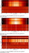 |
Fig. A.1 Data detrending procedure for an example spectral order (exposures versus wavelengths) from HARPS (panel a), NIRPS (panel b), and CRIRES+ (panel c). Each panel shows the following steps: A-the raw time series of a single spectral order during the transit; B-after continuum normalisation; C-after dividing out the median out-of-transit spectrum; D — final residuals after removing stellar and telluric spectral lines using the principal component analysis. |
Appendix B Correction for stellar effects
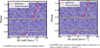 |
Fig. B.1 Iron cross-correlation trail maps for HARPS optical data exhibiting non-negligible stellar contamination (i.e. Rossiter-McLaughlin effect) at the systemic velocity expected from Delrez et al. (2016). Dashed yellow lines define the transit window. The solid red line illustrates the Keplerian curve (i.e. the planet’s orbital motion). Panel (a) shows the HARPS optical data not corrected for the stellar contamination as Doppler shadow, while panel (b) shows the Doppler shadow masked (corresponding flux values are set to NaN and discarded). |
All Tables
Prior and posterior planetary parameter distributions obtained with juliet for WASP-121.
WASP-121b SCARLET atmospheric posteriors from the retrieval analysis on the HARPS, NIRPS, and CRIRES+ time series combined.
Mass reference. We computed ΔKp assuming different stellar masses by keeping the stellar reflex motion fixed.
All Figures
|
Fig. 1 Observing conditions as a function of phase. The blue, orange, yellow, and green points correspond to NIRPS (and simultaneous HARPS) observations, while the pink and black points represent CRIRES+ observations in the H- and K-bands, respectively. Top panel and mid panel illustrate the airmass and the average atmospheric Dimm seeing (i.e. value for the differential image monitor) evolving during the nights, respectively. The Dimm seeing is averaged for each observations (i.e. average between the start and the end of each observation). The bottom panel shows the signal-to-noise ratio (extracted from the fits header) changing during the nights. |
| In the text | |
|
Fig. 2 Simultaneous photometry with EulerCam. Top: detrended EulerCam light curves with the best-fit transit models overlaid on top. Bottom: residuals for each observation. The horizontal dashed lines indicate the continuum at zero. |
| In the text | |
|
Fig. 3 Top panel: radial velocity time series (coloured dots) and best-fit Keplerian model (grey line) for the juliet fit of the WASP-121 public RVs. The fitted instrumental offsets μinstrument have been subtracted from each time series. Bottom panel: residuals of the fit. |
| In the text | |
|
Fig. 4 Top panel: phase-folded RVs (coloured dots) and best-fit Keplerian model (black line). The colours of the RV points match those in Fig. 3. Both the fitted instrumental offsets and the GP components (where applicable) have been subtracted from each time series. Bottom panel: residuals of the fit. |
| In the text | |
|
Fig. 5 Top panel: stacked phase-folded TESS photometry (grey dots), binned data for each sector (coloured dots), and best-fit model (black line) for the juliet fit of the WASP-121 TESS photometry. Bottom panel: residuals of the fit. |
| In the text | |
|
Fig. 6 Atmospheric models (transit depth as function of wavelength) for OH (brown), Fe (green), V (magenta), CO (red), H2O (blue), and TiO (orange) generated with the SCARLET code. The shaded regions highlight the spectral coverage of each instrument. The range of the wavelength of HARPS is in yellow, the NIRPS region is in cyan, and the CRIRES+ H-band and K-band are in purple and orange, respectively. |
| In the text | |
|
Fig. 7 Detections of CCFs for Fe (SNR=5.8), CO (SNR=5.0), and V (SNR=4.7), and non-detection of H2O (SNR<2.0) in the transmission spectrum of WASP-121b. Each squared panel shows the two-dimensional cross-correlation map in the velocity-velocity space (Kp − Vsys). The white dashed lines indicate the expected position of the planetary signal within the velocity-velocity space, namely the expected orbital (~216 km s−1, Hoeijmakers et al. 2024) and systemic (3 8.35 ± 0.02 km s−1, Delrez et al. 2016) velocities of WASP-121b. The rectangular panels on top depicts the one-dimensional cross-correlation of each species as signal-to-noise ratio versus systemic velocity. Detections of Fe and V are primarily driven by the optical HARPS observations, while the CO detection by the infrared CRIRES+ data (mostly K-band observations). |
| In the text | |
|
Fig. 8 Key retrieved results. The four distributions represent the probability density of retrieved chemical abundance ratios (in logarithmic scale). Overplotted the FastChem model predictions in chemical equilibrium as varying the metallicity and the C/O ratio. FastChem theoretical models are displayed as function of the pressure in bar. |
| In the text | |
|
Fig. 9 Retrieved constraints on the atmospheric and orbital properties from HARPS, NIRPS and CRIRES+ combined transits of WASP-121b. We assumed a free atmospheric retrieval condition and hence a well-mixed chemistry (constant with altitude). |
| In the text | |
|
Fig. 10 Vecolity offset, ΔKp, as a function of different stellar masses. This plot serves to visualise the Table 6 in comparison with global circulation model predictions. Each data point with uncertainties corresponds to the computed ΔKp as a function of the stellar mass (reported in Table 6) as derived by Delrez et al. (2016) (M⋆ = 1.35 ± 0.08 M⊙), Borsa et al. (2021) (M⋆ = 1.38 ± 0.02 M⊙), Sing et al. (2024) (M⋆ = 1.33 ± 0.02 M⊙), and Prinoth et al. (2025) (M⋆ = 1.42 ± 0.03 M⊙), respectively. Uncertainties are calculated via error propagation. Vertical lines mark the GCM predictions, namely models with zero, weak, and strong drag by Tan et al. (2024) and drag-free models by Parmentier et al. (2018). |
| In the text | |
|
Fig. A.1 Data detrending procedure for an example spectral order (exposures versus wavelengths) from HARPS (panel a), NIRPS (panel b), and CRIRES+ (panel c). Each panel shows the following steps: A-the raw time series of a single spectral order during the transit; B-after continuum normalisation; C-after dividing out the median out-of-transit spectrum; D — final residuals after removing stellar and telluric spectral lines using the principal component analysis. |
| In the text | |
|
Fig. B.1 Iron cross-correlation trail maps for HARPS optical data exhibiting non-negligible stellar contamination (i.e. Rossiter-McLaughlin effect) at the systemic velocity expected from Delrez et al. (2016). Dashed yellow lines define the transit window. The solid red line illustrates the Keplerian curve (i.e. the planet’s orbital motion). Panel (a) shows the HARPS optical data not corrected for the stellar contamination as Doppler shadow, while panel (b) shows the Doppler shadow masked (corresponding flux values are set to NaN and discarded). |
| In the text | |
Current usage metrics show cumulative count of Article Views (full-text article views including HTML views, PDF and ePub downloads, according to the available data) and Abstracts Views on Vision4Press platform.
Data correspond to usage on the plateform after 2015. The current usage metrics is available 48-96 hours after online publication and is updated daily on week days.
Initial download of the metrics may take a while.