| Issue |
A&A
Volume 703, November 2025
|
|
|---|---|---|
| Article Number | A242 | |
| Number of page(s) | 15 | |
| Section | Numerical methods and codes | |
| DOI | https://doi.org/10.1051/0004-6361/202556339 | |
| Published online | 20 November 2025 | |
Interpreting the detection of anomalies in SDSS spectra
1
Departamento de Física, Universidad de Antofagasta
Avenida Angamos 601,
Antofagasta,
Chile
2
Université Côte d’Azur, Observatoire de la Côte d’Azur, CNRS, Laboratoire Lagrange,
06000
Nice,
France
★ Corresponding authors: This email address is being protected from spambots. You need JavaScript enabled to view it.
; This email address is being protected from spambots. You need JavaScript enabled to view it.
Received:
10
July
2025
Accepted:
29
September
2025
Abstract
Context. The increasing use of machine-learning methods in astronomy introduces important questions about interpretability. The complexity and nonlinear nature of machine-learning methods means that it can be challenging to understand their decision-making process, especially when applied to the detection of anomalies. While these models can effectively identify unusual spectra, it remains a great challenge to interpret the physical nature of the flagged outliers.
Aims. We aim to bridge the gap between an anomaly detection and the physical understanding by combining deep learning with interpretable machine-learning (iML) techniques to identify and explain anomalous galaxy spectra from SDSS data.
Methods. We present a flexible framework that uses a variational autoencoder to compute multiple anomaly scores, including physically motivated variants of the mean-squared error. We adapted the iML LIME algorithm to spectroscopic data, systematically explored segmentation and perturbation strategies, and computed explanation weights that identified the features that are most likely to cause a detection. To uncover population-level trends, we normalized the LIME weights and applied clustering to 1% of the most strongly anomalous spectra.
Results. Our approach successfully separated instrumental artifacts from physically meaningful outliers and grouped anomalous spectra into astrophysically coherent categories. These include dusty metal-rich starbursts, chemically enriched H II regions with moderate excitation, and extreme emission-line galaxies with a low metallicity and hard ionizing spectra. The explanation weights agree with established emission-line diagnostics and enable a physically grounded taxonomy of spectroscopic anomalies.
Conclusions. Our work shows that an interpretable anomaly detection provides a scalable, transparent, and physically meaningful approach to exploring large spectroscopic datasets. Our framework opens the door for incorporating interpretability tools into quality control, follow-up targeting, and discovery pipelines in current and future surveys.
Key words: methods: data analysis / methods: miscellaneous / methods: statistical
© The Authors 2025
 Open Access article, published by EDP Sciences, under the terms of the Creative Commons Attribution License (https://creativecommons.org/licenses/by/4.0), which permits unrestricted use, distribution, and reproduction in any medium, provided the original work is properly cited.
This article is published in open access under the Subscribe to Open model. This email address is being protected from spambots. You need JavaScript enabled to view it. to support open access publication.
1 Introduction
The recent advances in instrumentation and telescope technology (Moravec et al. 2019; Siemiginowska et al. 2019), have ushered in an era of abundance for astronomy. This abundance poses new challenges. The traditional knowledge-discovery process does not scale well in this scenario of big and complex data. For instance, the Vera Rubin Legacy Survey of Space and Time (LSST) is estimated to deliver about 500 Petabytes worth of data (Ivezić et al. 2019). In this context, the use of machine-learning (ML) methods is gaining momentum.
Among the many types of ML algorithms, deep neural networks (DNNs) are becoming ubiquitous. While their flexibility and the affinity of these models with GPUs has made them prime choices for addressing many challenges, employing them often comes at the expense of interpretability: The nonlinear interactions between the features of the data and the different parameters of DNNs make the problem intractable in most cases. This opacity, often referred to as the black-box problem, is a widely recognized challenge in applying advanced artificial intelligence (AI) to scientific domains because it can hinder trust, verification, and reproducibility (Adadi & Berrada 2018; Molnar 2020; Biecek & Burzykowski 2021; Li et al. 2025; Wetzel et al. 2025; Lieu 2025). In this sense, DNNs are black boxes.
The field of interpretable machine-learning (iML) methods, or explainable AI (XAI), aims to demystify these complex models and to provide human-friendly explanations for the predictions of a model. Because ML is increasingly adopted in astronomy, iML techniques are becoming a requirement for ensuring that AI-driven research remains reliable, transparent, and aligned with scientific principles. The use of iML in science facilitates the debugging and improvement of models, builds trust by verifying that predictions are based on sound and well-established physics and phenomenology, and, most importantly, it accelerates knowledge acquisition by providing insights into the underlying processes a model has learned from data, which might lead to new hypotheses and discoveries (Adadi & Berrada 2018; Sahakyan 2024; Wetzel et al. 2025).
Recent years have seen a growing interest in applying iML techniques in astronomy. Use cases spanned galaxy morphology, spectroscopic classification, photometric redshift estimation, and cosmology. These methods fall into two main categories. The first category includes model-specific explanations, which are intrinsically tied to the architecture or training process of the model itself (Yip et al. 2021; Jacobs et al. 2022; Bhambra et al. 2022; Lucie-Smith et al. 2022; Gully-Santiago & Morley 2022; Pandey et al. 2023; Bonse et al. 2025). The second category comprises model-agnostic post hoc methods, such as local interpretable model-agnostic explanations (LIME, Ribeiro et al. 2016) and Shapley additive explanations (SHAP, Lundberg & Lee 2017; Lundberg et al. 2020), which can be applied to any predictive model. Within this class, SHAP-based studies have been used to understand model behavior across applications including SED modeling, galaxy clustering, molecular abundance prediction, and cosmological parameter inference (Gilda et al. 2021; Machado Poletti Valle et al. 2021; Villaescusa-Navarro et al. 2022; Dey et al. 2022; Heyl et al. 2023b,a; Crupi et al. 2024; Elvitigala et al. 2024; Grassi et al. 2025; Ye et al. 2025). On the other hand, LIME-based approaches have been used in studies of strong emission-line galaxies, black hole accretion, and cosmological model selection (Dold & Fahrion 2022; Pasquato et al. 2024; Ocampo et al. 2025). Together, these efforts show the growing role of iML in astronomy and its potential to improve trust, transparency, and scientific interpretability.
The detection of anomalies represents a particularly compelling application for iML. With continuously growing data volumes, the ability to automatically flag outliers in surveys such as the Sloan Digital Sky Survey (SDSS), Gaia, or LSST becomes critical for identifying rare or unexpected phenomena. The field has advanced significantly with the development of unsupervised and self-supervised ML methods that detect outliers in images, spectra, and time-series data (e.g., Baron & Poznanski 2017; Reis et al. 2018; Ichinohe & Yamada 2019; Giles & Walkowicz 2020; Lochner & Bassett 2021; Vafaei Sadr et al. 2023; Ciprijanović et al. 2023; Etsebeth et al. 2024; Aleo et al. 2024; Lochner & Rudnick 2025; Semenikhin et al. 2025; Kornilov et al. 2025). The detection alone is insufficient for scientific insight, however. Many flagged outliers remain poorly characterized, and the sheer volume of candidates overwhelms efforts of manual inspection. In this context, iML offers a promising solution by helping us to diagnose why an object is considered anomalous. It high-lights the features that contribute most to the anomaly score. This not only improves trust and interpretability, but also enables astronomers to prioritize the most compelling candidates.
We present a new and flexible public tool for easily performing an explainable anomaly detection on spectroscopic observations based on LIME. In Sect. 2 we present the SDSS Data Release 16 (DR16) spectroscopic sample we used and the data-cleaning procedures we performed in preparation for the anomaly-detection algorithm that we introduce in Sect. 3. We detail the LIME algorithm adaptation for an interpretable anomaly detection in Sect. 4 before we present the results in Sect. 5 and discuss them in Sect. 6. We conclude in Sect. 7.
2 Sample selection and data processing
We adopted the SDSS DR16 spectroscopic dataset of galaxies. Its reasonably large size and excellent quality make it ideal for detecting an anomaly, as shown by Baron & Poznanski (2017).
The data and associated metadata were obtained from the skyserver data repository1. They yielded a total of 1 230 784 spectra from the sdss dataset. We shifted the spectra to their rest frame and interpolated them to a common grid in the optical region of 350–750 nm. High-redshift spectra have many missing values. To avoid this scenario, we constrained our sample to the redshift range between 0.01–0.50. As a consequence, we worked with a total of 791 738 spectra. To avoid contamination by the [OIλ557.7] line, we removed the wavelengths in the region of 556.5–559.0 nm from all spectra before we deredshifted them. Afterward, we removed wavelengths with a signal-to-noise ratio (S/N) lower than one. We also corrected for the Milky Way fore-ground extinction according to dust maps from Schlegel et al. (1998)2. After the spectra were corrected for the foreground extinction, we shifted them to rest frame and interpolated all the spectra to a common grid with a resolution of 0.1 nm. After the interpolation, we dropped all spectra with not-a-number (NaN) values higher than 10%. The final sample contained 728 133 spectra. The summary statistics for the redshift and median S/N of this sample are presented in Table 1.
To further refine the sample, we first dropped all wavelengths for which more than 10% of spectra have NaN values. This reduced the number of wavelength points per spectrum from 4000 to 3773. Because ML algorithms are sensitive to missing values and the dynamical range of the data, we replaced the NaNs for the remaining missing values in each individual spectrum with its median flux to ensure consistency. We then applied a median-flux normalization to each spectrum to bring them onto a common scale and mitigate the effect of absolute flux variations. Finally, considering that machine-learning algorithms are sensitive to noise levels, we divided the sample into four bins based on the median S/N of each spectrum. This binning helped us to homogenize noise properties and prevented the anomaly-detection model from identifying different noise levels as anomalous features. The first three bins contained 182 094 spectra each, and the fourth bin (highest S/N) contained 181 850 spectra. To develop the model, we used 80% of the spectra in each bin for the training and the remaining 20% for the validation (see Sect. 3.1).
Summary statistics for the redshift (z) and median S/N of the final sample.
3 Anomaly detection
Anomaly detection is a complex task, in particular with high dimensional data, as is the case of spectra with thousands of fluxes as features. In order to detect an anomaly, we need a measure of the similarity between different observations. An object is anomalous when it is dissimilar from the rest; in a scientific context, the goal is to identify which of these dissimilar objects are astrophysically interesting. This is a subjective task. In high dimensional spaces, the notion of distance is distorted. For instance, Aggarwal et al. (2001) showed that as the dimensionality of a space increases, the Euclidean metric is unable to discern between the farthest and the closest point to the origin of a dataset where all points are generated with a multidimensional uniform distribution. One implication of this result is that there is no single universal anomaly score that is capable of retrieving all types of anomalies, in particular, when we consider that the definition of a useful anomaly depends on the scientific goal. Similarly, the theorem of “no free lunches” from optimization theory states that there is no best model for performing a particular task (Wolpert & Macready 1997). This conclusion directly applies to the detection of an anomaly, for which there is no universal algorithm. Different algorithms will retrieve different types of anomalies (Nun et al. 2016; Reis et al. 2021).
We implemented an anomaly-detection framework based on variational autoencoders (VAEs), which are a type of NNs. VAEs can be considered as a black box that aims to reconstruct the most common features of spectra. As a consequence, spectra with anomalous features are poorly reconstructed (Ichinohe & Yamada 2019). One way to assign an anomaly score is to measure the distance between a spectrum and its reconstruction by the VAE. When we couple the VAE with a distance metric, we obtain a regression model that maps a spectrum to an anomaly score. We considered different distance metrics to mitigate the curse of dimensionality and be able to retrieve different types of anomalous spectra. While some authors identified anomalies as points in low-density regions of the VAE latent space (Portillo et al. 2020), we focused on the reconstruction error. This approach has the advantage of directly linking an anomaly score to specific misreconstructed features in the spectrum, which agrees with our goal of generating feature-based interpretations. In what follows, we describe VAEs and the distances we used to assign an anomaly score to a spectrum.
3.1 Variational autoencoders
The VAEs are neural networks that belong to the family of generative learning (GL) models in ML (Kingma & Welling 2013). GL models are designed to generate synthetic data (Goodfellow et al. 2016; Foster 2019). An example of the use of VAEs with spectra can be found in Portillo et al. (2020), who used them as a dimensionality-reduction technique that outperformed methods such as principal component analysis and non-negative matrix factorization. In addition, the authors used the lower dimensional representation obtained with VAEs for other downstream tasks, such as generating synthetic data or detecting an anomaly. A VAE is composed of an encoder network and a decoder network. The encoder outputs a lower dimensional vector representation of the input spectrum. This representation is also called the latent representation. The decoder takes the latent representation to produce a reconstruction of the original spectrum. Another possibility is to sample points from the latent space and generate new spectra with the decoder. VAEs, by their nature, also allow us to explore perturbations of the data used in the training phase (Engel et al. 2017). We describe the architecture and the training of the VAE in detail in Appendix A. While a detailed quantitative comparison with other anomaly-detection algorithms is beyond the scope of this paper, it is worth noting that VAEs have proven to be a robust method for this task in astronomy (e.g., Ichinohe & Yamada 2019; Portillo et al. 2020; Sánchez-Sáez et al. 2021; Liang et al. 2023; Rogers et al. 2024; Quispe-Huaynasi et al. 2025; Nicolaou et al. 2025). Our VAE performs well in its primary function: It successfully learns to reconstruct the spectra of typical galaxies from the SDSS dataset with low error, as exemplified in the top panel of Figure 1. Consequently, it produces poor reconstructions with high error for spectra containing features that are not well represented in the training data (Fig. 1, bottom panel). This behavior demonstrates that the VAE has effectively learned the underlying distribution of the data, which makes its reconstruction error a reliable proxy for an anomaly scoring.
3.2 Anomaly score
To obtain the anomaly score of a spectrum using the VAE, we followed the Algorithm 1.
First, we propagated the spectrum through the VAE and reconstructed it. To compute the anomaly score, we used the spectrum, X, and its reconstruction, X′. By nature, the most common features in the spectra will be well reconstructed and anomalous features will be poorly reconstructed (see Fig. 1 for examples of reconstructions with high and low anomaly scores).
Require: X ⊳X: observed spectrum
Require: VAE
Require: S ⊳ S: anomaly scoring function
X′ ← VAE .reconstruction(X) ⊳ X′: reconstruction of X
s ← S(X, X′) ⊳ s: outlier score of X return score
Then, the key ingredient is the metric to compute the distance, which under Algorithm 1 is the anomaly score S(X, X′). We explored eight anomaly scores, each derived by comparing a spectrum X with its reconstruction X′. These scores fall into two families depending on the underlying distance metric: the standard mean-squared error (MSE), and an inverse-flux weighted variant (χ2). The key idea is that poorly reconstructed features correspond to anomalous content, and each variation is designed to probe a different type of deviation.
The first family was based on the standard MSE metric (see Eq. (A.3)). We added three physically motivated variations to the MSE to probe different behaviors in spectra. For instance, we noted that the MSE has the tendency to highlight as anomalous spectra with strong standard emission lines and data glitches. Strong emission lines are anomalous in the sense that they are rare in our data, but they are objects that in most cases are known, such as startburst galaxies. On the other hand, data glitches are often due to either cosmic rays or instrumental errors. These spectra are anomalous in the same sense as spectra with strong emission lines, but they do not constitute interesting anomalies. The variations we introduced to mitigate the prevalence of these anomalous patterns are listed below.
-
Filtered MSE: this masks common emission lines before the residuals are computed. This variation mitigates the dominance of strong emission lines. The filtered MSE is defined as
 (1)
(1)where fi corresponds to the filter and takes the value of one for fluxes at wavelengths outside the filtered region, and zero otherwise. The width of the filter is defined by ∆λ = λl∆υ/c, with λl the wavelength of the line, c is the speed of light, and ∆υ the velocity width of the masking window. The filtered lines are given in Table B.1.
Trimmed MSE: this removes the top 3% highest residuals before the MSE is computed. This helps suppress the influence of localized glitches, such as cosmic rays or bad pixels.
Filtered + trimmed MSE: this applies line masking and trimming. This combination targets subtle continuum-level anomalies while avoiding common strong features and data artifacts.
Together with the unmodified MSE, these yield four total MSE-based scores. The second family uses an inverse-flux weighted MSE that effectively computes the χ2 between the observation and the reconstruction,
 (2)
(2)
where δ is a positive and low value. We introduced δ to avoid division by zero. This score naturally downweights residuals in bright regions (e.g., strong emission lines), making it complementary to standard MSE. As with MSE, we defined three additional variants: (1) Filtered χ2, (2) trimmed χ2, and (3) filtered + trimmed χ2. Together with the baseline χ2 score, this yields four additional χ2-based scores for the total of eight anomaly-scoring functions we used in our analysis.
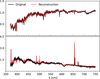 |
Fig. 1 Example of a good (upper panel) and poor (lower panel) reconstruction by the VAE. The MSE score for the good reconstruction is ≈0.00019, and for the poor reconstruction, it is ≈0.015. The fluxes are median normalized. |
4 Interpretable machine-learning with LIME
It is essential to understand what drives the anomaly score for an object for the scientific validation, knowledge discovery, and error diagnosis. Interpretable machine-learning provides tools and methods for verifying that ML-driven conclusions agree with physical expectations. These methods can be broadly categorized into model-specific and model-agnostic techniques. Model-specific approaches, such as decision trees and integrated gradients in neural networks (Sundararajan et al. 2017), have an inherent interpretability. In contrast, model-agnostic approaches, such as SHAP (Lundberg & Lee 2017) and LIME (Ribeiro et al. 2016), can be applied to any ML model without modifying its internal structure. We introduce the LIME-spectra-interpreter, which is an adaptation of LIME for interpreting an anomaly detection in spectroscopic data. We show that when anomaly is detected, the intuition we gain with the LIME-spectra-interpreter can help us to automate the insight by highlighting the features that are correlated to the anomaly score of an object. To explain a prediction, LIME approximates the complex model with a surrogate that is easier to interpret. We considered the case of linear surrogates. An interesting point about LIME is that the space of features of the interpreter is different from the space of features of the model we wish to inspect.
The algorithm LIME is traditionally used for image and tabular data by perturbing input features (pixels or table columns) and training a simple surrogate model to approximate the complex ML model locally. In an image analysis, LIME groups neighboring pixels into superpixels and then selectively removes information to determine the feature importance. Our adaptation, the LIME-spectra-interpreter, extends this idea to spectroscopic data by using spectral segments. Instead of grouping neighboring pixels in an image, we segment spectra into wavelength bins, which can be defined either uniformly or using clustering techniques such as SLIC (Achanta et al. 2010). For instance, the interpreter uses segments of the spectrum as predictors and not a single wavelength. These segments constitute what Ribeiro et al. (2016); Molnar (2020) and Biecek & Burzykowski (2021) denominated human-friendly or meaningful representations of the data. The perturbation process then modifies spectral regions (e.g., by adjusting flux values or adding noise) to examine the effect of these changes on the anomaly scores.
To explain the model, LIME perturbs the original data to obtain a new set of spectra. These new spectra are then used to fit the interpreter that approximates the original model. The process of obtaining perturbed spectra makes use of the segmented representation of the spectrum. To generate a new spectrum, LIME randomly selects a subset of segments and grays them out. All perturbed wavelengths can be set to either a hard coded value defined by the user or to the mean value of their respective segment.
In mathematical terms, the segmented representation of a perturbed spectrum Z can be considered as a binary vector Z′, where each entry labels a segment. A one (zero) value in the ith entry of Z′ means that the ith segment of Z is not perturbed (perturbed). When we denote the interpreter by 𝑔, then the interpreter has the form
 (3)
(3)
where N is the number of segments, and  is the ith entry of Z′. The weights of the linear model indicate the importance of each segment. Because of the random nature of the perturbation process, some spectra are very dissimilar from the original, which might harm the ability of the interpreter to locally approximate the model in the vicinity of the original spectrum. To mitigate this effect, LIME weights the proximity of a perturbation to the original spectrum using an exponential kernel that is given by
 (4)
(4)
where D(x, z) is the distance between the original spectrum and the perturbation z. By default, LIME uses the L2 norm.
Finally, when we call our model f, then the weights of the interpreter are found by minimizing the loss function,
 (5)
(5)
where 𝒵 is the set of perturbed spectra and their segment representation.
In summary, our adaptation of LIME for spectroscopic data involves two key modifications. First, instead of image superpixels, we segment spectra into meaningful wavelength regions using either uniform divisions or clustering-based methods. Second, instead of masking pixels, we perturb the data by scaling fluxes and replacing segments with their mean flux or fixed values to probe the sensitivity of the model to specific features.
Throughout this work, we adopt the following default configuration: a flux scaling as in the perturbation method with a scale factor of 0.9, a uniform segmentation (each section indicates the number of segments), and 5000 perturbed samples. These settings balance interpretability, resolution, and computational efficiency (see Sect. 6.2).
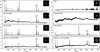 |
Fig. 2 Overview of SDSS anomalies identified by different variations of the MSE score. Each row displays example spectra (with SDSS imaging thumbnails) that we found using the respective MSE variation (e.g., MSE or trimmed MSE), with two representative examples per variation. The different MSE variations effectively highlight different anomalous patterns in the spectra. The fluxes are median normalized. |
5 Results
5.1 Overview of anomaly score findings
Our anomaly detection framework computed eight anomaly scores: four scores derived from the MSE, and four from inverse-flux weighting (χ2), each incorporating optional filtering and trimming strategies (Sect. 3.2) for each SDSS spectrum. Through the inspection of the top anomalous spectra, we found that different scoring metrics emphasized distinct spectral characteristics and revealed a variety of astrophysical and instrumental anomalies. We present a sample of anomalous spectra in Fig. 2.
The MSE metric (top row) primarily identifies spectra with strong emission-line features, particularly in the [OIII] and Hα regions. This suggests a sensitivity to extreme star-forming galaxies, in which these emission lines dominate the flux distribution. Additionally, MSE detects spectra with data artifacts.
When the MSE score was computed after ignoring 3% of the highest residuals (second row), its focus shifted toward anomalies with unusual continua. This modification reduced the sensitivity to extreme flux variations and instead highlighted objects with peculiar stellar populations or spectra that do not correspond to a typical galaxy.
A 250 km s−1 filter applied to the locations of standard emission lines (third row) further refined the selection by prioritizing spectra with broader emission lines. This variation detected anomalies that likely correspond to turbulent star-forming regions or AGNs. On the other hand, the sensitivity to data artifacts was also increased by filtering out standard emission lines.
Finally, combining the velocity filter with residual suppression (bottom row) resulted in a diverse set of anomalies that included both emission-line sources and spectra with moderate continuum deviations. A direct comparison of these metrics shows that only 4% (14.8%) of the top 100 (1000) anomalies are common across all different scores, which reinforces our finding that the anomaly scores are sensitive to different behaviors in spectra. This result is consistent with the results of other studies that reported little overlap between different methods for detecting an anomaly (Reis et al. 2021), even when only variations in the MSE were considered and the metrics were not completely different.
5.2 Interpretable anomaly detection: Matching anomalies to astronomical intuition
Beyond identifying outliers, we assessed whether the explanation weights provided by our framework agreed with the interpretation of an astronomer of the anomalous spectra. To do this, we analyzed four of the anomalies illustrated in Fig. 2 using the explanation weights obtained with our LIME-based approach. The selected spectra and their explanations are shown in Fig. 3.
The object in panel a exhibits exceptionally strong and narrow emission lines, with [OII] λλ372.7, 372.9, [OII] λλ495.9, 500.7,Hβ, and Hα dominating the spectrum. These lines reach flux levels that are ≈20 times stronger than the continuum, suggesting the presence of a starburst. The LIME explanation weights plotted below the spectrum confirm this interpretation: The highest weights are sharply peaked at the exact locations of the most prominent emission lines, especially [OII], [OIII], Hβ, and Hα. This outcome illustrates that the anomaly score is driven by physically meaningful features that would naturally be identify as unusual. The interpreter therefore provides a transparent justification for the anomaly score decision of the model. This again provides confidence that the framework agrees with domain expertise.
By contrast, the spectrum in panel b highlights a different class of anomalies that is not tied to extreme astrophysical properties, but instead to data-quality issues: a forest of irregular high-frequency fluctuations across the redder wavelengths, with a sharp discontinuity near λ ≈750 nm. These features lack a coherent physical structure and do not correspond to known spectral lines. This suggests the presence of noise or poor sky subtraction. In this case, the LIME weights are concentrated precisely in the problematic red part of the spectrum, which confirms that the anomaly score is dominated by the noisy segment. This would manually be classified as an observational artifact and not as a genuine astrophysical outlier. The interpreter correctly identifies the region of concern, even in an unphysical case. This demonstrates that the model and explanation can be used not only to highlight meaningful features, but also to flag unreliable data products.
In panel c, we analyze a spectrum that was flagged as anomalous using the MSE score with a 250 km s−1 filter applied around the locations of standard emission lines (Table B.1). At first glance, the spectrum appears to be dominated by classic nebular emission features such as [OII] λλ372.7,372.9, [OII] λ500.7, Hβ, and Hα. This object stands out not simply because of the strength of the lines, but because their profiles are unusually broad. The explanation weights reinforce this interpretation. They peak precisely at the locations of these broad features, which indicates that the anomaly score is driven not only by the flux amplitude, but by the width and structure of the lines. This behavior matches expectations, as the applied filter suppresses narrow lines and enhances sensitivity to broader features, such as those associated with turbulent star-forming regions or possible AGN activity. The agreement between the score, the explanation, and the astrophysical interpretation offers a compelling validation of the interpreter’s ability to highlight relevant anomaly-driving features.
Finally, in panel d, we examine an anomalous spectrum that was identified using the MSE score filtered at 250 km s−1 and further refined by ignoring the top 3% of the reconstruction residuals from the VAE. This spectrum stands out for its atypical structure. To the left of Hα, the flux distribution shows irregular broadening, while toward the blue end, just short of the 400 nm break, there is a dip-like flux suppression that deviates from the standard galaxy continuum. The LIME explanation weights confirm that these regions dominate the anomaly score, with high weights concentrated in the vicinity of the 650–670 nm region and in the 380–400 nm range. The ability of the interpreter to isolate these regions helps us to narrow the interpretation space and guides further scrutiny. This outcome strongly agrees with the goals of an interpretable anomaly detection.
These case studies illustrate the value of integrating explanation mechanisms with anomaly detection in spectra. In each example, the LIME-spectra-interpreter correctly highlighted the spectral regions that an astronomer would identify as the cause for the anomaly, whether based on extreme emission features, broadened line profiles, continuum deviations, or potential data artifacts. This agreement between algorithmic reasoning and expert intuition builds trust in the framework and demonstrates that the model is not only effective at flagging unusual spectra, but is also capable of offering interpretable justifications that facilitate scientific insight and follow-up analysis.
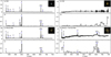 |
Fig. 3 Explanations of four representative anomalies detected with different MSE-based scores, each showing the median normalized flux (top. with an SDSS imaging thumbnail) and corresponding maximum normalized LIME explanation weights (bottom). The panels show: (a) an extreme emission-line object driven by [OIII] and Hα peaks (MSE), (b) the red-end weighting from likely instrumental noise (MSE), (c) a broad emitter with high weights on Hα and [OII] (filtered MSE), and (d) continuum deviations near Hα and the 400 nm break (filtered + trimmed MSE). The explanations consistently highlight features driving the anomaly. This agrees with astronomers’ interpretations. |
5.3 General trends in anomalies
Sections 5.1 and 5.2 demonstrated that different variations of the MSE-based anomaly score and the LIME-explanation weights are sensitive and highlight diverse anomalous patterns in spectra, including strong emission-line galaxies, unusual continua, and data artifacts. To move from individual case studies to population-level insights, we now analyze global trends using clustering over LIME explanation weights. We focus on the top 1% most anomalous spectra as measured by the standard MSE score, that is, on 1818 spectra.
Since LIME produces individualized explanations per spectrum, the scale and sign of the weights can vary significantly across the sample. To make these explanations comparable, we focused on the strength of the contribution of each feature using its absolute value and normalized each explanation vector to unit length. This transformation ensured that we focused on explanation patterns without being affected by differences in scale. We used the KMeans clustering algorithm from the scikit-learn3 library. KMeans is an unsupervised clustering algorithm that partitions data into clusters by minimizing the intracluster sum of square Euclidean distances (inertia). It iteratively assigns each point to the nearest cluster centroid and updates centroids based on the mean of the assigned points until convergence.
To obtain an optimal number of clusters, we applied the elbow method, which plots the inertia against the number of clusters and identifies a point from which adding more clusters yields diminishing returns. We also complemented the elbow method with the silhouette score, which measures the similarity of an object to its own cluster compared to other clusters. A higher silhouette score indicates better-defined clusters. It is worth mentioning that under the unit length normalization of the explanation weights, the Euclidean distance behaves similarly to the cosine similarity. Therefore, we minimized the curse of dimensionality when clustering the explanation weights. We found that seven clusters are adequate for a meaningful partitioning of the top 1% anomalies. We summarize the cluster distribution in Table 2.
We organize our discussion by grouping the clusters into three categories: (i) artifact-driven outliers (clusters 0 and 5), (ii) hybrid cases that blend physical signals with data-processing artifacts (clusters 4 and 6), and (iii) physically rich emission-line populations (clusters 1, 2, and 3). Figures 4, 5 and 6 show the average spectrum and explanation for each cluster.
The inspection of the clustering output reveals that clusters 0 and 5 primarily capture outliers dominated by observational or data-reduction artifacts. For cluster 0, the left upper panels of Fig. 4 show that these spectra exhibit common emission features such as Hα, Hβ, and [OIII] on average. Nonetheless, the LIME explanation weights reveal that the anomaly score is not driven solely by these lines. Instead, the average explanation shows a broad uneven structure across the continuum, with an increasing trend at the blue end of the spectrum. The cumulative importance of the region blueward of 450 nm exceeds that of the main emission lines. A visual inspection of the top 20 ranked anomalous spectra confirms recurring data artifacts and high-frequency noise around the 400 nm break and the [OII] λ372.7 regions. A similar pattern emerges in cluster 5. The right upper panels of Fig. 4 show that the average explanation is diffuse and fails to target any specific spectral feature. A visual inspection of the top-ranked anomalies shows spectra dominated by single sharp spikes at a random wavelengths, with otherwise flat or featureless continua. Overall, the outliers in these two clusters are not driven by physical processes in galaxies, but rather by data-reduction errors or isolated instrumental anomalies. This result highlights the discriminative power of the LIME-based framework to isolate systematic outliers. It offers an automatic quality-control layer for future spectroscopic explorations.
Clusters 4 and 6, in the left and right bottom panels of Fig. 4, represent a second category where the detected anomalies reflect a combination of physical structure and data-processing artifacts. Both clusters are characterized by strong [OIII] λ500.7 emission, but this line appears to be partially clipped across the spectra. Upon closer inspection, we identified the origin of this effect: During preprocessing, prior to de-redshifting, the region between 556.5–559.0 nm was masked in all spectra to remove contamination from the strong night-sky line [OI] λ557.7. Because clusters 4 and 6 have median redshifts of z = 0.1083 and z = 0.1181, respectively, the [OIII] λ500.7 feature overlaps with this masked region, which results in systematic truncation. The LIME explanation weights consistently assign the highest importance to this region, indicating that the clustering successfully identifies a coherent anomaly pattern rooted in preprocessing artifacts. While the clipping prevents a reliable estimation of excitation line ratios, the spectra in both clusters nonetheless show strong nebular emission and structured continua. Photometric inspection reveals predominantly compact morphologies that are consistent with small actively star-forming galaxies. This case illustrates how explanation-based clustering can disentangle subtle combinations of physical signals and systematic effects. This offers a useful diagnostic for both astrophysical interpretation and data-quality control.
Finally, we studied clusters 1, 2, and 3, which account for 34%, 16%, and 19% of the top 1% most anomalous spectra, respectively. Together, they comprise 69% of the sample and correspond to physically interesting systems. As shown in Fig. 5 and 6, the average spectra in these clusters all exhibit rich nebular emission features, including the Balmer series, [OIII] λλ495.9, 500.7, and [OII] λ372.7, and low-ionization lines such as [NII] and [SII]. While these signatures broadly indicate active star formation, their spectral subtleties and LIME explanation profiles reveal distinct physical regimes across clusters. Overall, the structured feature attributions in the LIME explanations indicate different line ratios as the key drivers of the anomaly scores. In clusters 1–3, the Balmer decrement ranges from 3.43 to 3.93 (Table 3), indicating non-negligible dust attenuation.
Cluster 1 (left panels in Fig. 5) shows a strong LIME emphasis at Hα+[NII], with additional attributions (similar) to Hβ, [OIII], [OII], and [SII]. Its line ratios, [NII]/Hα (0.26–0.32) and O3N2 (0.53–0.69), suggest a moderate metallicity. The [OIII]/[OII] ratio (1.06–1.32) indicates a moderately hard radiation field. A visual inspection of the SDSS imaging reveals that the top 20 ranked anomalies in this cluster are compact blue star-forming galaxies. This is consistent with the spectroscopic interpretation of this cluster as a population of moderate-excitation enriched H II regions with active star formation.
Cluster 2 (right panels in Fig. 5) exhibits a more line-balanced explanatory pattern dominated by [OII] λ372.7, with more evenly distributed weights across other features. The diagnostic ratios, [NII]/Hα (0.17–0.21), [OIII]/Hβ (1.58–1.86), and [OIII]/[OII] (1.24–1.48), imply a harder ionizing field and lower metallicities than cluster 1. The SDSS photometry for the top 20 ranked anomalies in this cluster shows a more morphologically diverse population than cluster 1. Several galaxies appear to be inclined or are seen edge-on, which is suggestive of disk-like morphologies. A number of systems are compact and relatively symmetric, but generally less blue and concentrated than those in cluster 1. The colors vary, with some objects displaying bluer tones that are indicative of ongoing star formation, while others show redder hues that may reflect older stellar populations. In summary, the photometric diversity in cluster 2 agrees well with its moderate- to high-excitation spectral features. This cluster seems to contain a mix of low-metallicity star-forming spirals and compact galaxies, possibly at more evolved or varied evolutionary stages than those in cluster 1.
In contrast, cluster 3 (Fig. 6) isolates galaxies with stronger excitation conditions than the previous clusters. The average spectrum is dominated by [OIII] λ500.7 in flux and explanation weight. Secondary explanation importance is assigned to Hα+[NII], Hβ, [OIII] λ495.9, and [OII]. Its [OIII]/Hβ (3.13–3.53), [OIII]/[OII] (2.54–3.06), and O3N2 (1.23–1.37) ratios exceed those of the other clusters, while [NII]/Hα drops (0.11–0.15). These values indicate low-metallicity systems with hard ionizing fields. The SDSS images of the top 20 ranked anomalies in cluster 3 show predominantly compact blue-dominated morphologies that are consistent with high surface brightness star-forming regions. Many exhibits round or slightly irregular shapes, with little evidence of extended structure or disk components. A few galaxies display asymmetric light distributions or faint tidal features that might indicate interactions or bursts triggered by mergers. The uniformity in their compactness and color further supports the interpretation of these systems as low-metallicity extreme emission-line galaxies, possibly similar to Green Pea analogs or high-ionization starburst galaxies (e.g. Cardamone et al. 2009).
Together, these three clusters demonstrate the power of explanation-driven anomaly detection to uncover astrophysical diversity. Despite their broadly similar emission-line spectra, the LIME-based clustering enables the separation of galaxies into physically coherent subsets that range from dusty moderately enriched bursts (cluster 1) to lower-metallicity moderate-excitation systems (cluster 2) and extreme low-metallicity emitters with hard ionizing fields (cluster 3).
To provide a more concrete connection to these galaxies, we present the spectra and corresponding optical imaging for a selection of interesting anomalies from these three clusters in Appendix C. While we focused on establishing the method and validating it against known astrophysical phenomena, these examples show that the framework has the potential for scientific discovery by highlighting a diverse range of compelling and extreme objects.
Distribution of the top 1% most anomalous spectra across explanation-based clusters.
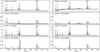 |
Fig. 4 Average spectrum and LIME explanation weights for clusters 0, 5, 4, and 6 from the top 1% most anomalous spectra (MSE score). Clusters 0 and 5 (top rows) show diffuse or noisy explanations with low weights, which is consistent with poor continuum reconstructions or spikes. Clusters 4 and 6 (bottom rows) feature strong weights at truncated [OIII] λ500.7 lines due to masked regions during preprocessing. This illustrates how explanation-based clustering isolates artifacts from astrophysical signals. The fluxes are median normalized. |
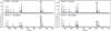 |
Fig. 5 Average spectrum and LIME explanation weights for clusters 1 and 2 of the top 1% most anomalous spectra (MSE score). Cluster 1 (left panels) emphasizes Hα+[NII] and [OIII], consistent with dusty metal-rich starbursts. Cluster 2 (right panels) highlights [OII]λ372.7, indicating moderate-excitation enriched H II regions. Clustering by explanation profiles reveals distinct physical regimes within spectrally similar galaxies. The fluxes are median normalized. |
Emission line diagnostics for clusters 1–3.
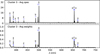 |
Fig. 6 Average spectra and LIME explanation weights for cluster 3 of the top 1% most anomalous spectra (MSE score). Cluster 3 is dominated by [O III]λ500.7, which is characteristic of extreme low-metallicity systems. As discussed for clusters 1 and 2, clustering by explanation profiles reveals distinct physical regimes within spectrally similar galaxies. The fluxes are median normalized. |
6 Discussion
6.1 Interpretation speed
The latest generation of large surveys in astronomy will generate massive amounts of data and produce numerous alerts as they find anomalies in near real time. Tools such as the one we presented will be increasingly essential for exploring these alerts efficiently and for helping astronomers triage and interpret them. To illustrate the practical feasibility of our method, we measured the explanation generation time. On a standard notebook with an AMD Ryzen 7 PRO 5850U CPU, LIME produces one explanation in approximately 0.82 s per core. Scaling this to a dataset of one million spectra results in a total runtime of roughly 9.5 days on a single core. With basic parallelization, for example, 100 parallel jobs on a small computing cluster, however, this time drops to ≈2.3 hours. These results show that our interpretability framework is scalable and well suited for integration into high-throughput pipelines.
6.2 Effects of segmentation and perturbation
The LIME explanations depend on several hyperparameters, including the type of perturbation, the segmentation strategy, the number of segments, and the number of perturbed samples used to fit the local surrogate model. These choices can significantly affect the resulting explanations. In the remainder of this section, we systematically assess the sensitivity of LIME explanations to each parameter by varying them independently while keeping the others fixed to their default values (Sect. 4).
6.2.1 Perturbation
The perturbation strategy plays a critical role in how LIME assigns explanation weights to different spectral regions. Our default approach was to apply a flux scaling within randomly selected segments. This perturbation preserves local flux structures and agrees with the interpolation capabilities of neural networks. This method is robust across a range of scaling factors. Fig. 7 shows the explanation weights for a spectrum when scaling factors of 0.6, 0.9 (default), and 1.2 were applied. The overall attribution pattern remains qualitatively consistent, particularly in the continuum. This suggests that the explanations are stable against moderate changes in scaling magnitude.
We then tested flat perturbations, in which each segment was replaced by a constant value to gray its signal out. Because all the spectra were median-normalized, a natural baseline was 1.0. Figure 8 compares this to values of 0.8 and 1.2 and shows that small deviations introduce spurious continuum attributions. In contrast, using 1.0 yields results closest to the scaling-based explanations, which confirms it as the most neutral choice.
We also tested a variant in which each segment was replaced by its mean flux, which removed local structure while preserving the global level. The left panel of Fig. 9 shows that this perturbation highlights sharp emission and absorption lines, while continuum regions receive fewer attributions. An explanation peak around 517.5 nm arises from missing data, which illustrates the sensitivity of this method to flux contrasts. To further explore this behavior, we applied this scheme to a spectrum dominated by sky-subtraction artifacts and to another with strong emission lines (middle and right panel in Fig. 9). In both cases, the explanations correctly highlight the unusual features in each case, but broader attribution patterns are more difficult to interpret. This method can be helpful in diagnosing artifact-dominated spectra or probing flux ratios, but it requires caution.
In summary, the perturbation method has a substantial effect on the resulting explanations. Scaling-based perturbations provide stable interpretable results that preserve local structure and are most consistent with the training distribution of the model. Flat or mean-based perturbations can be informative in specific contexts, but risk injecting artifacts or suppressing physically meaningful features.
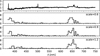 |
Fig. 7 Explanation weights under different flux scaling perturbations of 0.6, 0.9 (default), and 1.2. The overall structure is stable across scale factors. The fluxes are median normalized, and the weights are factors of 10−2. |
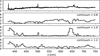 |
Fig. 8 Explanation weights using flat perturbation values of 0.8, 1.0, and 1.2. The value of 1.0 (third panel; the median-normalized flux) yields coherent results, while deviations (second and fourth panels) introduce spurious continuum weights. The fluxes are median normalized, and the weights are factors of 10−2. |
6.2.2 Segmentation
Two key parameters govern the segmentation of the input spectrum for perturbation-based explanation: the number of segments, and the number of perturbed samples. These parameters are interdependent because the number of segments defines the dimensionality of the local neighborhood that the interpreter must sample. Specifically, given n segments, the number of possible perturbed combinations is 2n − 1. A small number of segments results in fewer degrees of freedom and requires fewer samples to fit the surrogate model. Conversely, a larger number of segments expands the combinatorial space, demanding more samples to faithfully approximate the local behavior of the model. Fewer segments often group together physically distinct regions (e.g., continuum and emission lines), however, which might reduce or eliminate the interpretability. At the other extreme, too many segments may lead to overfitting or include segment sizes that are smaller than the spectral resolution; an ill-posed scenario. Figure 10 illustrates these trade-offs using uniform segmentation (left panel) and SLIC segmentation (right panel). The uniform segmentation divides the spectrum into equal-width segments, while SLIC uses a clustering approach to adaptively determine segment boundaries based on flux structure.
In both segmentation schemes, explanations with very few segments tend to concentrate weights over broad continuum regions and fail to isolate specific features. With many segments (e.g., >942), explanations become noisy and less structured. Notably, the SLIC segmentation with an upper bound of 111 (yielding 54 segments) produces an explanation that captures the anomalous continuum structure of this spectrum. It is interesting to note that the SLIC segmentation with an upper bound of 943 segments yields 1058 segments, which is more than the number of segments in the uniform segmentation. This results in a very noisy explanation because the segments are too small to capture meaningful flux variations.
We also explored the effect of the number of perturbed samples on the explanation quality. Fig. 11 shows explanations using 100, 1000, and 5000 perturbed spectra under a uniform segmentation of 77 segments. With only 100 samples, the interpreter produces noisy and unreliable weights. At 1000 samples, the structure begins to emerge with little continuum noise. Finally, at 5000 samples, the explanation is stable and agrees with the anomalous nature of this spectrum. This emphasizes that under high-dimensional perturbation spaces, sufficient sampling is essential to suppress artifacts and recover faithful attributions.
6.3 Interpretable machine-learning in astronomy
As machine-learning becomes ubiquitous in astronomy, extending interpretability frameworks to accommodate different astronomical data types is increasingly important. We demonstrated that model-agnostic explainability tools such as LIME can be successfully adapted to spectroscopic data to provide physically grounded insights into anomaly-detection results. In our case, two core components were adapted: segmentation, and perturbation. Instead of pixel-based superpixels used in image tasks, we segmented galaxy spectra into wavelength intervals uniformly or via clustering. Perturbations, instead of masking or replacing features, involve flux rescaling within segments, which preserves the spectral structure in a way that is compatible with anomaly detection. This modularity highlights the broader flexibility of LIME. The same framework might, in principle, be extended to other astronomical domains. For instance, time series can be sliced into temporal segments, similar to spectral segments. Photometric data can be explained using passbands or color indices as interpretable features. Data cubes, such as ΓFU (Integral Field Unit) observations, present a more complex case, but can be segmented spatially and spectrally to assess local and global contributions to predictions. These generalizations are especially relevant in the context of ongoing and upcoming large-scale surveys such as LSST, DESI, and 4MOST, which, combined, will produce massive volumes of multimodal data that require scalable and interpretable analysis tools.
We showed that interpretable anomaly detection is not just viable, but powerful: The explanation weights align with astro-physical intuition, and the clustering of the explanations reveals structured trends in the top anomalies. This opens the door for automated prioritization, classification, and debugging work-flows that are transparent and scientifically meaningful.
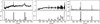 |
Fig. 9 Explanation weights using the mean flux of a segment as perturbation. Left: example spectrum from earlier sections. Middle: Artifact-dominated object. Right: Strong emission line galaxy. While this method highlights prominent lines effectively, it may also amplify flux gaps or downweight continua. The segmentation used 77 segments (left, middle) and 150 segments (right). The fluxes are median normalized, and the weights are max normalize. |
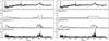 |
Fig. 10 Effect of the segment count on the explanation quality. Left: Uniform segmentation with 11, 111, and 943 segments. Right: SLIC segmentation with equivalent upper bounds, yielding 4, 54, and 1058 segments. Having too few segments dilutes key features; having too many adds noise. Intermediate settings yield clearer and more meaningful explanations. The fluxes are median normalized, and the weights are factors of 10−2. |
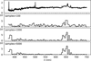 |
Fig. 11 Effects of the number of perturbed samples on the quality of the explanation. Explanations stabilize and improve as more perturbed samples are used. Too few samples yield noisy or misleading weights. The fluxes are median normalized and weights are factors of 10−2. |
7 Conclusions
We introduced a framework for an interpretable anomaly detection of SDSS galaxy spectra using a variational autoencoder (VAE) coupled with a customized LIME interpreter. Our key contributions include (1) a flexible VAE-based anomaly-scoring system using multiple reconstruction-based metrics, each capturing distinct types of spectral deviations. (2) A spectral adaptation of LIME that segments spectra into interpretable wavelength regions and applies perturbations through flux scaling, enabling local explanations of anomaly scores. (3) A systematic analysis of segmentation and perturbation choices, with default parameters selected to balance resolution and stability. (4) Clustering of LIME explanation weights for the top 1% most anomalous spectra, revealing astrophysically meaningful subgroups that agree with known emission line diagnostics and morphological traits.
By providing an interpretation of why spectra are anomalous, our framework connects the complex outputs from our model with expert-driven astrophysical insights. The explanations isolate features such as strong emission lines, continuum irregularities, and instrumental artifacts and enable automatic categorization and quality control. Our clustering analysis further demonstrates that the explanation space encodes rich physical structure, distinguishing dusty starbursts, chemically enriched H II regions, and extreme low-metallicity emitters. This work illustrates how interpretable ML can scale to large spectro-scopic datasets and deliver insights beyond an anomaly score to guide follow-up science and model development. The method can be generalized to other domains in astronomy to support the broader integration of explainability in the data-driven era of astronomy.
Data availability
All code used in this work is publicly available under an open-source license and can be found at the GitHub link in the footnote4. The organization hosts modular repositories for each component: data processing (sdss), VAE training (autoencoders), anomaly scoring (anomaly), and LIME-based explanation of spectra (xai-astronomy). Code is written in Python, with dependencies and usage instructions provided in each repository to ensure reproducibility.
Acknowledgements
EO belongs to the PhD Program Doctorado en Física, mención Física-Matemática, Universidad de Antofagasta, Antofagasta, Chile, and acknowledges support from the National Agency for Research and Development (ANID)/Scholarship Program/DOCTORADO BECAS NACIONAL CHILE/2018-21190387. MB acknowledges support from the ANID BASAL project FB210003. This work was supported by the French government through the France 2030 investment plan managed by the National Research Agency (ANR), as part of the Initiative of Excellence of Université Côte d’Azur under reference number ANR-15-IDEX-01.
References
- Achanta, R., Shaji, A., Smith, K., et al. 2010, EPFL Technical Report 149300 [Google Scholar]
- Adadi, A., & Berrada, M. 2018, IEEE Access, 6, 52138 [Google Scholar]
- Aggarwal, C. C., Hinneburg, A., & Keim, D. A. 2001, in Database Theory, ICTD 200, 8th International Conference, London, UK, January 4–6, 2001, 8, 15 [Google Scholar]
- Aleo, P. D., Engel, A. W., Narayan, G., et al. 2024, ApJ, 974, 172 [Google Scholar]
- Baron, D., & Poznanski, D. 2017, MNRAS, 465, 4530 [NASA ADS] [CrossRef] [Google Scholar]
- Bhambra, P., Joachimi, B., & Lahav, O. 2022, MNRAS, 511, 5032 [Google Scholar]
- Biecek, P., & Burzykowski, T. 2021, Explanatory Model Analysis (New York: Chapman and Hall/CRC) [Google Scholar]
- Bonse, M. J., Gebhard, T. D., Dannert, F. A., et al. 2025, AJ, 169, 194 [Google Scholar]
- Cardamone, C., Schawinski, K., Sarzi, M., et al. 2009, MNRAS, 399, 1191 [NASA ADS] [CrossRef] [Google Scholar]
- Chen, X., Kingma, D. P., Salimans, T., et al. 2016, arXiv e-prints [arXiv:1611.02731] [Google Scholar]
- Ciprijanovic, A., Lewis, A., Pedro, K., et al. 2023, Mach. Learn. Sci. Technol., 4, 025013 [Google Scholar]
- Crupi, R., Dilillo, G., Della Casa, G., Fiore, F., & Vacchi, A. 2024, Galaxies, 12, 12 [Google Scholar]
- Dey, B., Andrews, B. H., Newman, J. A., et al. 2022, MNRAS, 515, 5285 [NASA ADS] [CrossRef] [Google Scholar]
- Dold, D., & Fahrion, K. 2022, A&A, 663, A81 [NASA ADS] [CrossRef] [EDP Sciences] [Google Scholar]
- Elvitigala, A., Navaratne, U. d., Rathnayake, S., & Dissanayaka, K. 2024, in 2024 9th International Conference on Information Technology Research (ICITR), 1 [Google Scholar]
- Engel, J., Hoffman, M., & Roberts, A. 2017, arXiv e-prints [arXiv:1711.05772] [Google Scholar]
- Etsebeth, V., Lochner, M., Walmsley, M., & Grespan, M. 2024, MNRAS, 529, 732 [Google Scholar]
- Foster, D. 2019, Generative Deep Learning (O’Reilly Media, Inc.) [Google Scholar]
- Géron, A. 2017, Hands-On Machine Learning with Scikit-Learn and TensorFlow, 2nd edn., 4 (O’Reilly Media, Inc.), 10 [Google Scholar]
- Gilda, S., Lower, S., & Narayanan, D. 2021, ApJ, 916, 43 [NASA ADS] [CrossRef] [Google Scholar]
- Giles, D. K., & Walkowicz, L. 2020, MNRAS, 499, 524 [NASA ADS] [CrossRef] [Google Scholar]
- Goodfellow, I., Bengio, Y., & Courville, A. 2016, Deep Learning (MIT Press), http://www.deeplearningbook.org [Google Scholar]
- Grassi, T., Padovani, M., Galli, D., et al. 2025, A&A, 702, A71 [NASA ADS] [CrossRef] [EDP Sciences] [Google Scholar]
- Gully-Santiago, M., & Morley, C. V. 2022, ApJ, 941, 200 [Google Scholar]
- Heyl, J., Butterworth, J., & Viti, S. 2023a, MNRAS, 526, 404 [NASA ADS] [CrossRef] [Google Scholar]
- Heyl, J., Viti, S., & Vermariën, G. 2023b, Faraday Discuss., 245, 569 [Google Scholar]
- Ichinohe, Y., & Yamada, S. 2019, MNRAS, 487, 2874 [CrossRef] [Google Scholar]
- Ivezic, Ž., Kahn, S. M., Tyson, J. A., et al. 2019, ApJ, 873, 111 [NASA ADS] [CrossRef] [Google Scholar]
- Jacobs, C., Glazebrook, K., Qin, A. K., & Collett, T. 2022, Astron. Comput., 38, 100535 [NASA ADS] [CrossRef] [Google Scholar]
- Kingma, D. P., & Welling, M. 2013, arXiv e-prints [arXiv: 1312.6114] [Google Scholar]
- Kornilov, M. V., Korolev, V. S., Malanchev, K. L., et al. 2025, Astron. Comput., 52, 100960 [Google Scholar]
- Li, G., Lu, Z., Wang, J., & Wang, Z. 2025, arXiv e-prints [arXiv:2502.15388] [Google Scholar]
- Liang, Y., Melchior, P., Hahn, C., et al. 2023, ApJ, 956, L6 [Google Scholar]
- Lieu, M. 2025, Universe, 11, 187 [Google Scholar]
- Lochner, M., & Bassett, B. A. 2021, Astron. Comput., 36, 100481 [NASA ADS] [CrossRef] [Google Scholar]
- Lochner, M., & Rudnick, L. 2025, AJ, 169, 121 [Google Scholar]
- Lucie-Smith, L., Adhikari, S., & Wechsler, R. H. 2022, MNRAS, 515, 2164 [Google Scholar]
- Lundberg, S., & Lee, S.-I. 2017, arXiv e-prints [arXiv: 1705.07874] [Google Scholar]
- Lundberg, S. M., Erion, G., Chen, H., et al. 2020, Nat. Mach. Intell., 2, 2522 [Google Scholar]
- Machado Poletti Valle, L. F., Avestruz, C., Barnes, D. J., et al. 2021, MNRAS, 507, 1468 [CrossRef] [Google Scholar]
- Molnar, C. 2020, Interpretable Machine Learning (lulu.com) [Google Scholar]
- Moravec, E., Alpasian, M., Amon, A., et al. 2019, in BAAS, 51, 8 [Google Scholar]
- Nicolaou, C., Nathan, R. P., Lahav, O., et al. 2025, arXiv e-prints [arXiv:2506.17376] [Google Scholar]
- Nun, I., Protopapas, P., Sim, B., & Chen, W. 2016, AJ, 152, 71 [NASA ADS] [CrossRef] [Google Scholar]
- Ocampo, I., Alestas, G., Nesseris, S., & Sapone, D. 2025, Phys. Rev. Lett., 134, 041002 [Google Scholar]
- Pandey, C., Angryk, R. A., Georgoulis, M. K., & Aydin, B. 2023, Lect. Notes Comput. Sci., 14276, 567 [CrossRef] [Google Scholar]
- Pasquato, M., Trevisan, P., Askar, A., et al. 2024, ApJ, 965, 89 [NASA ADS] [CrossRef] [Google Scholar]
- Patel, A. A. 2019, Hands-On Unsupervised Learning Using Python: How to Build Applied Machine Learning Solutions from Unlabeled Data, 2nd edn., 4 (O’Reilly Media, Inc.), 10 [Google Scholar]
- Portillo, S. K. N., Parejko, J. K., Vergara, J. R., & Connolly, A. J. 2020, AJ, 160, 45 [Google Scholar]
- Quispe-Huaynasi, F., Roig, F., Holanda, N., et al. 2025, AJ, 169, 332 [Google Scholar]
- Reis, I., Poznanski, D., Baron, D., Zasowski, G., & Shahaf, S. 2018, MNRAS, 476, 2117 [CrossRef] [Google Scholar]
- Reis, I., Rotman, M., Poznanski, D., Prochaska, J. X., & Wolf, L. 2021, Astron. Comput., 34, 100437 [NASA ADS] [CrossRef] [Google Scholar]
- Ribeiro, M. T., Singh, S., & Guestrin, C. 2016, in Proceedings of the 22nd ACM SIGKDD International Conference on Knowledge Discovery and Data Mining, KDD ’16 (New York, NY, USA: Association for Computing Machinery), 1135 [Google Scholar]
- Rogers, B., Lintott, C. J., Croft, S., Schwamb, M. E., & Davenport, J. R. A. 2024, AJ, 167, 118 [Google Scholar]
- Sahakyan, N. 2024, arXiv e-prints [arXiv:2412.10093] [Google Scholar]
- Sánchez-Sáez, P., Lira, H., Martí, L., et al. 2021, AJ, 162, 206 [CrossRef] [Google Scholar]
- Schlegel, D. J., Finkbeiner, D. P., & Davis, M. 1998, ApJ, 500, 525 [Google Scholar]
- Semenikhin, T. A., Kornilov, M. V., Pruzhinskaya, M. V., et al. 2025, Astron. Comput., 51, 100919 [Google Scholar]
- Shafkat, I. 2018, Intuitively Understanding Variational Autoencoders, https://towardsdatascience.com/intuitively-understanding-variational-autoencoders-1bfe67eb5daf, accessed: 2022-05-08 [Google Scholar]
- Siemiginowska, A., Eadie, G., Czekala, I., et al. 2019, BAAS, 51, 355 [Google Scholar]
- Sundararajan, M., Taly, A., & Yan, Q. 2017, arXiv e-prints [arXiv: 1703.01365] [Google Scholar]
- Vafaei Sadr, A., Bassett, B. A., & Sekyi, E. 2023, RAS Tech. Instrum., 2, 586 [Google Scholar]
- Villaescusa-Navarro, F., Ding, J., Genel, S., et al. 2022, ApJ, 929, 132 [NASA ADS] [CrossRef] [Google Scholar]
- Wetzel, S. J., Ha, S., Iten, R., Klopotek, M., & Liu, Z. 2025, arXiv e-prints [arXiv:2503.23616] [Google Scholar]
- Wolpert, D., & Macready, W. 1997, IEEE Trans. Evol. Computat., 1, 67 [Google Scholar]
- Ye, S., Cui, W.-Y., Li, Y.-B., Luo, A. L., & Jones, H. R. A. 2025, A&A, 697, A107 [NASA ADS] [CrossRef] [EDP Sciences] [Google Scholar]
- Yip, K. H., Changeat, Q., Nikolaou, N., et al. 2021, AJ, 162, 195 [NASA ADS] [CrossRef] [Google Scholar]
- Zhao, S., Song, J., & Ermon, S. 2017, arXiv e-prints [arXiv:1706.02262] [Google Scholar]
Appendix A VAE architecture
The architecture of a VAE is defined with the number of layers in the encoder, the decoder, and the dimensionality of latent space. Each layer is defined by a set of neurons. The input of a neuron is the output of the neurons in the previous layer. The neuron performs a dot product of its inputs with a vector of weights, then it adds a bias term. The results of these operations is the input of an activation function. In this work we use the standard Rectified Linear Unit (ReLU) function,
 (A.1)
(A.1)
where max represents the maximum value between 0 and x. The output of a neuron is the output of the activation function.
We trained our VAE following standard procedures (Géron 2017; Patel 2019). Shortly, we define a loss function, a training and a validation set, and a criterion to stop training. The loss function guides the learning process of the VAE during the training phase. During training, batches of spectra from the training set are feed to the VAE. The reconstructions and latent representations of each batch are used to compute the loss function. If the loss function is not reduced, then the parameters of the VAE are updated using the back propagation algorithm (Géron 2017; Patel 2019). In this work, we used the Adam optimization algorithm for back propagation. The algorithm completes a training epoch when all the batches accounting for the training are feed to the model. The training finishes when the value of the loss function on the validation set does not drop during 10 epochs. It is worth remarking that the validation set contains different spectra from the training set, and it is used as a control set to avoid overfitting of the training set. In this work we train our VAE with spectra from SDSS DR16, see Sect. 2. The training and validation set contain 80% and 20% of the spectra of a given bin, respectively.
The loss function is given by the following equation,
 (A.2)
(A.2)
The loss function in Eq. A.2 contains three terms. A reconstruction term defined by the Mean Squared Error,
 (A.3)
(A.3)
where N represents the number of fluxes in a spectrum, denoted by X,and xi denotes a single flux of X. The MSE drives the VAE reconstruction power and helps to encode similar spectra onto clusters in the latent space (Shafkat 2018).
The second term is the Kullback-Leibler Divergence (KLD) (Kingma & Welling 2013),
![Mathematical equation: ${{\rm{D}}_{{\rm{KL}}}}\left( {q\left( w \right)\parallel p\left( w \right)} \right) = {{\rm{E}}_{q\left( w \right)}}\left[ { - \log \left( {{{q\left( w \right)} \over {p\left( w \right)}}} \right)} \right],$](/articles/aa/full_html/2025/11/aa56339-25/aa56339-25-eq10.png) (A.4)
(A.4)
where q(w) and p(w) are the probability distribution of the encoder and the prior for the decoder respectively. Finally, 𝔼q(w) is the expected value over q(w).
The last term is Maximum Mean Discrepancy (MMD) (Zhao et al. 2017),
![Mathematical equation: $\matrix{ {{\rm{MMD}}\left( {q\left( w \right)\parallel p\left( w \right)} \right) = {{\rm{E}}_{q\left( w \right),p\left( {w'} \right)}}\left[ {k\left( {w,\,w'} \right)} \right]} \cr { + {{\rm{E}}_{q\left( w \right),q\left( {w'} \right)}}\left[ {k\left( {w,\,w'} \right)} \right]} \cr { - 2{{\rm{E}}_{p\left( w \right),q\left( {w'} \right)}}\left[ {k\left( {w,\,w'} \right)} \right],} \cr } $](/articles/aa/full_html/2025/11/aa56339-25/aa56339-25-eq11.png) (A.5)
(A.5)
where w is the latent representation of a spectrum and w′ is a vector with the same dimension of w but sampled from prior of the decoder.
The KLD and MDD act as regularization terms to improve smoothness on the latent space (Zhao et al. 2017; Shafkat 2018). A smooth latent space is what makes VAEs generative models, since they allow a meaningful interpolation among points in it. A VAE with only the MSE, is an Auto Encoder (AE). An AE does not guarantee that an interpolation over empty regions in latent space will generate realistic spectra, therefore limiting its capabilities. This is because these gaps contain points not seen by the model during the training phase. To alleviate this situation, in conjunction with the MMD and KLD terms, VAEs incorporate a stochastic layer. This layer samples each spectrum over a distribution in the latent space during training. For this work, we use a multivariate Gaussian distribution, where its means and variances are trainable parameters of the model. In the training process, the VAE will see each spectrum several times. Therefore, thanks to this layer, each point will be sampled over a small region of latent space, rather than to a single point. Given this stochastic layer, the encoder network constitutes a distribution on the latent space, that is, the encoding distribution. As mentioned before, this distribution is represented by q(w), and the prior for the decoder by p(w). The objective of the KLD term is to make the encoder distribution in latent space similar to that of a normal distribution in a point by point fashion. Henceforth, the latent representation of the data is encouraged to be evenly distributed around the origin of the latent space. Finally, the MMD term, discourages the KL divergence to force the encoding distribution to match the prior, avoiding an uninformative latent space. The MMD term accomplishes this objective by encouraging the encoding distribution to match the prior p(w) of the decoder in expectation (Chen et al. 2016; Zhao et al. 2017). This is accomplished using a kernel function k(w, w′) as shown in Eq. A.5. The kernel function measures the similarity between two samples, in this case, a sample of w from the encoding distribution and sample of w′ from the prior of the decoder, in our case a multivariate normal distribution. We used a Gaussian kernel,
 (A.6)
(A.6)
where the variance of the kernel was defined as the inverse of the dimensionality in the latent space, following recommendations in Zhao et al. (2017).
To select our models, first we defined different architectures, and for each we performed a grid search for α and λ. Among the different architectures, we found that the model with the best reconstructions have three layers in the encoder and the decoder and a latent dimension of 12. The number of neurons per layer, including the latent space, is given by 256 − 128 − 64 − 12 − 64 − 128 − 256. The values of α and λ for the best performing model trained on the bin with the largest S/N are 0 and 8.6 respectively.
Appendix B Lines
Narrow emission lines used in filters for anomaly scores
Appendix C Interesting anomalies from Cluster analysis
This appendix showcases a selection of representative interesting anomalies from the three main physically driven clusters discussed in section 5.3. For each of the three main clusters, we present four representative galaxies to connect clusters’ properties derived from the LIME weights with their spectral characteristics, the features that drive the anomaly score, with the underlying physical state and morphology revealed by their optical imaging.
The galaxies presented in Figure C.1 are examples from cluster 1, confirming its nature as a collection of moderate-excitation, enriched H II regions. All four spectra showcase the key features identified from the cluster’s average properties: strong Balmer emission lines (Hδ, Hγ, Hβ) and a prominent Hα+[NII] that is the most dominant feature, consistent with the average LIME weights that peak in this region. This shared spectral signature points to a common physical driver of intense star formation. Interestingly, the examination of these individual anomalies reveals important nuances. While Ranks 1, 2, and 18 are archetypal members of this cluster with strong Hα emission and moderate [OIII]/Hβ ratios, Rank 5 stands out as a more extreme case. Its spectrum shows the strongest emission lines in this small sample, with the [OIII] line being significantly stronger than Hα, indicating a considerably higher ionization parameter than is typical for this group. This highlights the diversity within a single cluster and demonstrates how the method groups objects with broadly similar interpretation patterns, even with significant variations in line strength. The photometry in this sample provides additional context. The thumbnails in the upper right of each spectrum reveal that these class of anomalies are found in a variety of dynamically active systems, from the disturbed spiral of Rank 1 and a starburst in the spiral arms of Rank 18 to the clumpy edge-on disk of Rank 2. The particularly high-excitation spectrum of Rank 5 corresponds to an intensely blue and compact morphology, suggesting a concentrated and powerful starburst event.
The anomalies in cluster 2 (Fig C.2) represent a distinct population with a significantly higher ionization state compared to cluster 1. This is spectrally evident in two main ways across the examples. First, the [OIII] emission becomes much more prominent, being of similar strength, and in some cases stronger than Hα, as seen in the spectrum of Rank 11. This highlights the harder ionizing field characteristic of the cluster. Second, another key feature is the consistently strong [OII] emission, which aligns with the average LIME interpretation for this group being centered on this line. The photometry of these objects shows morphological evidence of gravitational interactions. This is evidenced by a diverse range of features, including the asymmetric “tadpole” structure of Rank 7, the large-scale warp in the disk of Rank 8, the chaotic morphology in Rank 11 pointing to a merger, and the tidal tails of the post-merger system in Rank 14.
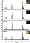 |
Fig. C.1 A selection of four representative anomalies from Cluster 1, which primarily consists of moderate-excitation, enriched H II regions. The sample highlights the diverse morphologies linked to this spectral class, including a disturbed spiral (Rank 1), an edge-on starburst (Rank 2), a compact galaxy (Rank 5), and an ongoing merger (Rank 18). The fluxes are median normalized. |
Finally, cluster 3 (Fig. C.3) represents the most spectrally extreme objects identified by our framework, consistent with the properties of rare “Green Pea” galaxies. All four spectra perfectly embody the defining characteristic of this class: they are overwhelmingly dominated by the [OIII] λλ495.9, 500.7 nm emission lines. This is a direct confirmation of the average LIME interpretation for this cluster, which peaks strongly on this feature. Furthermore, the characteristically low [NII]/Hα ratio, visible in all four panels, is a classic signature of the low-metallicity gas and hard ionizing radiation fields that define these systems. Photometry reveals that these extreme spectra originate in intensely blue and compact galaxies, with Rank 1 and 5 serving as archetypal examples. Rank 9 shows a chaotic merger while Rank 19 shows an interacting close pair of galaxies, suggesting that these extreme events are merger-triggered.
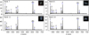 |
Fig. C.2 A selection of four representative anomalies from Cluster 2, characterized by harder ionizing fields and lower metallicities than Cluster 1. This cluster is characterized by a wide range of interaction-driven morphologies, including a “tadpole” galaxy (Rank 7), a warped disk (Rank 8), a chaotic merger (Rank 11), and a post-merger with tidal tails (Rank 14). Fluxes are median normalized. |
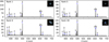 |
Fig. C.3 A selection of four representative anomalies from cluster 3, which isolates extreme emission-line, low-metallicity galaxies resembling “Green Pea” analogs. The examples showcase the compact, blue morphologies characteristic of this class, often found within interacting or merging systems. The fluxes are median normalized. |
Taken together, these examples illustrate interesting anomalous spectra and one of the utilities of our interpretable frame-work. It not only groups anomalies by their statistical properties but also successfully separates them into astrophysically coherent classes of anomalies as discussed in Section 5.3.
All Tables
Distribution of the top 1% most anomalous spectra across explanation-based clusters.
All Figures
|
Fig. 1 Example of a good (upper panel) and poor (lower panel) reconstruction by the VAE. The MSE score for the good reconstruction is ≈0.00019, and for the poor reconstruction, it is ≈0.015. The fluxes are median normalized. |
| In the text | |
|
Fig. 2 Overview of SDSS anomalies identified by different variations of the MSE score. Each row displays example spectra (with SDSS imaging thumbnails) that we found using the respective MSE variation (e.g., MSE or trimmed MSE), with two representative examples per variation. The different MSE variations effectively highlight different anomalous patterns in the spectra. The fluxes are median normalized. |
| In the text | |
|
Fig. 3 Explanations of four representative anomalies detected with different MSE-based scores, each showing the median normalized flux (top. with an SDSS imaging thumbnail) and corresponding maximum normalized LIME explanation weights (bottom). The panels show: (a) an extreme emission-line object driven by [OIII] and Hα peaks (MSE), (b) the red-end weighting from likely instrumental noise (MSE), (c) a broad emitter with high weights on Hα and [OII] (filtered MSE), and (d) continuum deviations near Hα and the 400 nm break (filtered + trimmed MSE). The explanations consistently highlight features driving the anomaly. This agrees with astronomers’ interpretations. |
| In the text | |
|
Fig. 4 Average spectrum and LIME explanation weights for clusters 0, 5, 4, and 6 from the top 1% most anomalous spectra (MSE score). Clusters 0 and 5 (top rows) show diffuse or noisy explanations with low weights, which is consistent with poor continuum reconstructions or spikes. Clusters 4 and 6 (bottom rows) feature strong weights at truncated [OIII] λ500.7 lines due to masked regions during preprocessing. This illustrates how explanation-based clustering isolates artifacts from astrophysical signals. The fluxes are median normalized. |
| In the text | |
|
Fig. 5 Average spectrum and LIME explanation weights for clusters 1 and 2 of the top 1% most anomalous spectra (MSE score). Cluster 1 (left panels) emphasizes Hα+[NII] and [OIII], consistent with dusty metal-rich starbursts. Cluster 2 (right panels) highlights [OII]λ372.7, indicating moderate-excitation enriched H II regions. Clustering by explanation profiles reveals distinct physical regimes within spectrally similar galaxies. The fluxes are median normalized. |
| In the text | |
|
Fig. 6 Average spectra and LIME explanation weights for cluster 3 of the top 1% most anomalous spectra (MSE score). Cluster 3 is dominated by [O III]λ500.7, which is characteristic of extreme low-metallicity systems. As discussed for clusters 1 and 2, clustering by explanation profiles reveals distinct physical regimes within spectrally similar galaxies. The fluxes are median normalized. |
| In the text | |
|
Fig. 7 Explanation weights under different flux scaling perturbations of 0.6, 0.9 (default), and 1.2. The overall structure is stable across scale factors. The fluxes are median normalized, and the weights are factors of 10−2. |
| In the text | |
|
Fig. 8 Explanation weights using flat perturbation values of 0.8, 1.0, and 1.2. The value of 1.0 (third panel; the median-normalized flux) yields coherent results, while deviations (second and fourth panels) introduce spurious continuum weights. The fluxes are median normalized, and the weights are factors of 10−2. |
| In the text | |
|
Fig. 9 Explanation weights using the mean flux of a segment as perturbation. Left: example spectrum from earlier sections. Middle: Artifact-dominated object. Right: Strong emission line galaxy. While this method highlights prominent lines effectively, it may also amplify flux gaps or downweight continua. The segmentation used 77 segments (left, middle) and 150 segments (right). The fluxes are median normalized, and the weights are max normalize. |
| In the text | |
|
Fig. 10 Effect of the segment count on the explanation quality. Left: Uniform segmentation with 11, 111, and 943 segments. Right: SLIC segmentation with equivalent upper bounds, yielding 4, 54, and 1058 segments. Having too few segments dilutes key features; having too many adds noise. Intermediate settings yield clearer and more meaningful explanations. The fluxes are median normalized, and the weights are factors of 10−2. |
| In the text | |
|
Fig. 11 Effects of the number of perturbed samples on the quality of the explanation. Explanations stabilize and improve as more perturbed samples are used. Too few samples yield noisy or misleading weights. The fluxes are median normalized and weights are factors of 10−2. |
| In the text | |
|
Fig. C.1 A selection of four representative anomalies from Cluster 1, which primarily consists of moderate-excitation, enriched H II regions. The sample highlights the diverse morphologies linked to this spectral class, including a disturbed spiral (Rank 1), an edge-on starburst (Rank 2), a compact galaxy (Rank 5), and an ongoing merger (Rank 18). The fluxes are median normalized. |
| In the text | |
|
Fig. C.2 A selection of four representative anomalies from Cluster 2, characterized by harder ionizing fields and lower metallicities than Cluster 1. This cluster is characterized by a wide range of interaction-driven morphologies, including a “tadpole” galaxy (Rank 7), a warped disk (Rank 8), a chaotic merger (Rank 11), and a post-merger with tidal tails (Rank 14). Fluxes are median normalized. |
| In the text | |
|
Fig. C.3 A selection of four representative anomalies from cluster 3, which isolates extreme emission-line, low-metallicity galaxies resembling “Green Pea” analogs. The examples showcase the compact, blue morphologies characteristic of this class, often found within interacting or merging systems. The fluxes are median normalized. |
| In the text | |
Current usage metrics show cumulative count of Article Views (full-text article views including HTML views, PDF and ePub downloads, according to the available data) and Abstracts Views on Vision4Press platform.
Data correspond to usage on the plateform after 2015. The current usage metrics is available 48-96 hours after online publication and is updated daily on week days.
Initial download of the metrics may take a while.