| Issue |
A&A
Volume 704, December 2025
|
|
|---|---|---|
| Article Number | A40 | |
| Number of page(s) | 29 | |
| Section | Galactic structure, stellar clusters and populations | |
| DOI | https://doi.org/10.1051/0004-6361/202452449 | |
| Published online | 02 December 2025 | |
How well can we unravel the accreted constituents of the Milky Way stellar halo?: A test on cosmological hydrodynamical simulations
1
Instituto de Astrofísica de Canarias,
38205
La Laguna, Tenerife,
Spain
2
Universidad de La Laguna, Dpto. Astrofísica,
38206
La Laguna, Tenerife,
Spain
3
Astrophysics Research Institute, Liverpool John Moores University,
146 Brownlow Hill,
Liverpool
L3 5RF,
UK
★ Corresponding author: This email address is being protected from spambots. You need JavaScript enabled to view it.
Received:
1
October
2024
Accepted:
29
September
2025
Abstract
Context. One of the primary goals of Galactic Archaeology is to reconstruct the Milky Way’s accretion history. To achieve this, significant efforts have been dedicated to identifying signatures of past accretion events. In particular, the study of the integrals of motion (IoM) space has proven to be highly insightful for uncovering these ancient mergers and understanding their impact on the Galaxy’s evolution.
Aims. This paper evaluates the effectiveness of a state-of-the-art method for detecting debris from accreted galaxies by testing it on four Milky Way-like galaxies from the Auriga suite of cosmological magnetohydrodynamic simulations.
Methods. We employed an innovative method to identify substructures in the IoM space within the local stellar halos of the four simulated galaxies. This approach enabled us to evaluate the method’s performance by comparing the properties of the identified clusters with the known populations of accreted galaxies in the simulations. Additionally, we investigated whether incorporating chemical abundances and stellar age information can help to link distinct structures originating from the same accretion event.
Results. This method is very effective in detecting debris from accretion events occurring less than 6–7 Gyr ago, but it struggles to detect most of the debris from older accretion. Furthermore, most of the detected structures suffer from significant contamination from in situ stars. Our results also show that the method might also generate artificial detections.
Conclusions. Our work shows that the Milky Way’s accretion history remains uncertain, while questioning the reality of some of the structures detected in the solar vicinity.
Key words: Galaxy: formation / Galaxy: halo / Galaxy: kinematics and dynamics / Galaxy: structure
© The Authors 2025
 Open Access article, published by EDP Sciences, under the terms of the Creative Commons Attribution License (https://creativecommons.org/licenses/by/4.0), which permits unrestricted use, distribution, and reproduction in any medium, provided the original work is properly cited.
This article is published in open access under the Subscribe to Open model. This email address is being protected from spambots. You need JavaScript enabled to view it. to support open access publication.
1 Introduction
In the current Λ cold dark matter cosmological model, the accretion of smaller satellite galaxies and interactions between galaxies play a fundamental role in the formation and evolution of galaxies. Indeed, large galaxies, such as the Milky Way (MW), grow hierarchically by accreting gas from cosmic filaments, which drives their secular evolution and leads to the formation of in situ stars, but also by cannibalising smaller satellite galaxies during successive accretion events (Eggen et al. 1962; Searle & Zinn 1978; White & Frenk 1991; Springel & Hernquist 2005; Carollo et al. 2007, 2010; Purcell et al. 2011; Qu et al. 2017). Therefore, it is fundamental to understand the relative importance of these two formation channels to shape the properties of galaxies as we see them today. Furthermore, determining the epoch of accretion of the accreted galaxies, and studying their internal properties (e.g. mass, luminosity, chemical evolution, star formation history, and associations with globular clusters or other galaxies) are essential for constraining cosmological models. However, the majority of the accretion events occurred in the early Universe (e.g. Blumenthal et al. 1984; Grand et al. 2017; Monachesi et al. 2019; Horta et al. 2023). As such, observing this process while it is ongoing at high redshift will likely remain unfeasible in the foreseeable future due to their inherently faint luminosity, even with cutting-edge instruments such as the James Webb Space Telescope (JWST). Although, it has recently been shown that the JWST can detect galaxy pairs prior to their merger for systems with stellar masses as low as 108 M⊙ (Duan et al. 2024), its use in studying these mergers remains limited. Therefore, the Galactic archaeology approach of uncovering past accretion and merger events by identifying the stars shed among those of the host galaxy is fundamental to complementing the work carried out with large galaxy samples, including those at high redshifts (e.g. Conselice 2014; Costantin et al. 2023), with the aim of developing a comprehensive understanding of the processes driving the formation and evolution of galaxies across different environments and epochs.
Over the lifetime of a large galaxy, the spatial coherence of an accreted galaxy is rapidly lost due to phase-mixing, especially for the most massive accreted galaxies. These massive galaxies, due to dynamical friction, quickly sink into the centre of the host, where the dynamical timescale is on the order of a few hundred million years (Amorisco 2017; Vasiliev et al. 2022). Even less massive galaxies situated in the outer stellar halo, where ongoing galaxy disruption can be observed in the form of stellar streams (see Amorisco 2017; Mateu 2023; Ibata et al. 2024, and references therein), typically lose their spatial coherence within a few billion years (Johnston et al. 2008; Gómez et al. 2010).
Despite this loss of spatial coherence, it was postulated that the remnants of accreted galaxies remain clustered in integrals of motion (IoM) space or in action space, which would still allow for the debris left by past accreted galaxies to be identified (Helmi & White 1999; Helmi & de Zeeuw 2000; Knebe et al. 2005; Brown et al. 2005; Font et al. 2006; McMillan & Binney 2008; Morrison et al. 2009; Gómez & Helmi 2010). Additionally, the chemical composition of individual stars serves as an additional tool for identifying the remnants of these accreted galaxies, as stars from the same galaxy share similar chemical abundance patterns (Freeman & Bland-Hawthorn 2002; Venn et al. 2004; Lee et al. 2015; Fernandes et al. 2023), which are somewhat distinct from those of stars formed in situ (e.g. Hawkins et al. 2015; Haywood et al. 2018; Das et al. 2020; Horta et al. 2021; Belokurov & Kravtsov 2022).
In this context, the MW offers a unique opportunity to study the accretion history of an individual galaxy. Not only is it a typical galaxy within the Local Universe (Kormendy et al. 2010; van Dokkum et al. 2013; Papovich et al. 2015; Bland-Hawthorn & Gerhard 2016), but it is also the only massive galaxy for which we can obtain full 6D phase-space information, detailed chemical abundances, and relative ages for large samples of individual stars. Although similar attempts have been made on other nearby galaxies within the Local Volume (e.g. Gilbert et al. 2014; D’Souza & Bell 2018; McConnachie et al. 2018; Mackey et al. 2019; Zhu et al. 2020; Davison et al. 2021), the MW remains unparalleled in the level of detail that can be achieved.
The ESA flagship mission Gaia (Gaia Collaboration 2018) provides accurate astrometry, parallaxes, proper motions, and even radial velocities and stellar parameters and chemical abundance (Recio-Blanco et al. 2023). These data can be complemented with ground-based spectroscopic surveys that provide radial velocities and chemical abundances for stars too faint for Gaia RVS, such as the Sloan Digital Sky Survey / Sloan Extension for Galactic Understanding and Exploration (SDSS/SEGUE; Yanny et al. 2009), Large Sky Area Multi-Object Fiber Spectroscopic Telescope (LAMOST; Zhao et al. 2012; Yan et al. 2022), RAdial Velocity Experiment (RAVE; Steinmetz et al. 2006, 2020b,a), Galactic Archaeology with HERMES (GALAH; Buder et al. 2021), Apache Point Observatory Galactic Evolution Experiment (APOGEE; Abdurro’uf et al. 2022), and the Gaia–European Southern Observatory Survey (Gaia-ESO; Gilmore et al. 2022; Randich et al. 2022) have collectively transformed our understanding of the Milky Way. These efforts will soon be complemented by new large-scale spectroscopic surveys such as the Dark Energy Spectroscopic Instrument Milky Way Survey (DESI-MWS; Cooper et al. 2023), William Herschel Telescope Enhanced Area Velocity Explorer (WEAVE; Dalton et al. 2012; Jin et al. 2024), 4-metre MultiObject Spectroscopic Telescope (4MOST; de Jong et al. 2019), and Sloan Digital Sky Survey V (SDSS-V; Kollmeier et al. 2017). These comprehensive data sets now make it possible to detect the dynamical debris left by past accreted galaxies, even if they do not form spatially coherent structures anymore (see Helmi 2020 and Deason & Belokurov 2024 for recent reviews).
With these data, numerous stellar debris associated with accreted galaxies have been discovered in the local stellar halo complementing already known debris, such as the Sagittarius dwarf galaxy (M⋆ = 108 M⊙ accreted ~4–6 Gyr ago; Ibata et al. 1994; Majewski et al. 2003; Niederste-Ostholt et al. 2010). These include Gaia-Enceladus-Sausage (GES; M⋆ = 108−1010 M⊙ accreted ~10 Gyr ago; Helmi et al. 2018; Vincenzo et al. 2019; Mackereth et al. 2019; Gallart et al. 2019; Feuillet et al. 2020; Naidu et al. 2022; Lane et al. 2023), Heracles-Kraken-IGS (M⋆ ~ 2 × 10⁸ M⊙ accreted ~11 Gyr ago; Kruijssen et al. 2019, 2020; Massari et al. 2019; Horta et al. 2021), Sequoia (M⋆ ~ 5 × 10⁷ M⊙ accreted ~9 Gyr ago; Myeong et al. 2018b, 2019; Naidu et al. 2020; Matsuno et al. 2022), the Helmi stream (Helmi & White 1999; Kepley et al. 2007; Koppelman et al. 2019b, M⋆ ~ 108 M⊙, accreted 5–9 Gyr ago), and Thamnos (M⋆ ~ 5 × 10⁶ M⊙, accreted > 10 Gyr ago; Koppelman et al. 2019a; Ruiz-Lara et al. 2022; Dodd et al. 2024). This list is far from exhaustive, and many recent studies have also identified smaller stellar substructures (e.g. LMS-1/Wukong, Pontus, Typhon/ED-4, ED-2-6, Shakti, Shiva, Rg5, Arjuna, L’Itoi, Nyx, L-RL64/Antaeus, etc.; Malhan et al. 2021; Malhan 2022; Naidu et al. 2020; Necib et al. 2020; Yuan et al. 2020; Myeong et al. 2022; Oria et al. 2022; Tenachi et al. 2022; Lövdal et al. 2022; Ruiz-Lara et al. 2022; Dodd et al. 2023); however, the accreted origins of some remain a matter of debate (e.g. Nyx and Aleph; Necib et al. 2020; Naidu et al. 2020; Zucker et al. 2021; Horta et al. 2023).
In most cases, the detection of these structures is carried out either through manual selection (e.g. Naidu et al. 2020; Oria et al. 2022; Tenachi et al. 2022) or by using clustering algorithms in dynamical or chemical space (e.g. Koppelman et al. 2019b; Myeong et al. 2022). However, the selection criteria used in manual methods, or the choice of parameters in clustering algorithms, can significantly influence which stars are assigned to a particular structure and might even alter the perceived properties of the structures themselves (Rodriguez et al. 2019; Carrillo et al. 2024). Machine learning techniques have also been employed to find clusters in IoM or action space (Yuan et al. 2018; Myeong et al. 2018a; Borsato et al. 2020; Shih et al. 2022) and have successfully identified various stellar streams. They were also used to separate accreted stars or globular clusters (Trujillo-Gomez et al. 2023) from those formed in situ (Veljanoski et al. 2019; Ostdiek et al. 2020; Tronrud et al. 2022; Sante et al. 2024). However, all these different methods have tat least one flaw and limitation; in particular, none of them are currently capable of measuring robustly the significance of each of these detections.
More recently, Lövdal et al. (2022) (hereafter L22) introduced a data-driven algorithm designed to detect and evaluate the significance of substructures in IoM space. This method is based on a single-linkage clustering approach and quantifies the number of stars grouped together by comparing them against a set of artificial background halos. What sets this technique apart is its ability to not only identify substructures but also to assign a robust statistical significance to each detection, while simultaneously providing insights into potential associations between distinct substructures by incorporating additional information such as the metallicity or the colour distribution. The effectiveness of this method has been demonstrated by its successful identification of new substructures in the IoM space within the local stellar halo of the MW (Ruiz-Lara et al. 2022; Dodd et al. 2023, hereafter RL22 and D23, respectively).
Another aspect to be considered is that the image d’Épinal of the preservation of the phase-space properties of the debris left by accreted galaxies and their significant chemical difference with in situ stars needs to be somewhat relativised. Cosmologically motivated simulations have demonstrated that a single accreted galaxy can give rise to multiple distinct structures in IoM or action space, which may further exhibit varying chemical distributions due to the underlying metallicity gradient in the original galaxy (Jean-Baptiste et al. 2017; Grand et al. 2019; Amarante et al. 2022; Khoperskov et al. 2023b,a; Mori et al. 2024). Conversely, the same simulations suggest that a given structure might result from the accumulation of stellar debris from multiple accretions or could be contaminated by in situ stars (Naidu et al. 2020; Orkney et al. 2022; Khoperskov et al. 2023a). Similar complexities have also been observed in groups of globular clusters (Pagnini et al. 2023).
In this paper, we assess the effectiveness of the L22 method in identifying structures and determining their significance using solar-neighbourhood-like stellar mocks derived from four MW-like galaxies from the Auriga suite of cosmological magnetohydrodynamic simulations (Grand et al. 2017, 2024). In Sect. 2, we present the properties of the primary progenitors of these four simulated galaxies. In Sect. 3, we describe the creation of the stellar halo mocks and introduces the L22 algorithm, including the modifications made to adapt it for use with the different mocks. The results of applying the algorithm to the mocks are analysed in Sect. 4. The properties of significant clusters are detailed in Sect. 4.1 and their chemical and age characteristics are thoroughly examined in Sect. 4.2. In Sect. 4.3, we investigate the purity and completeness of groups of dynamically close clusters, while Sect. 4.4 evaluates the algorithm’s effectiveness in scenarios lacking in situ stars. In Sect. 5, we explore the impact of artificial background halos on the significance of the detected clusters. Finally, in Sect. 6, we summarise our findings, discussing both the challenges inherent in the methods used for identifying and quantifying substructures, as well as the more intrinsic issues stemming from the initial expectations regarding the distribution in phase space and the chemical abundance patterns trends of accreted galaxies. We then used these insights to propose hypothetical properties of the accreted structures identified in the MW to date.
2 Data
2.1 Sample of Milky Way-like galaxies
We performed our analysis on a sample of high resolution gravo-magnetohydrodynamic cosmological zoom-in simulations of MW-mass halos (1 < M200/[1012 M⊙] < 2 at redshift 01) taken from the Auriga project (Grand et al. 2017). These simulations adopt the following cosmological parameters: Ωm = 0.307, Ωb = 0.048, ΩΛ = 0.693, σ8 = 0.8288, and a Hubble constant of H0 = 100 h km s−1 Mpc−1, where h = 0.6777, taken from Planck Collaboration XVI (2014). The initial conditions are generated for a starting redshift of 127, and follow the evolution of gas, dark matter, stars, and black holes down to a redshift of 0, according to a comprehensive galaxy formation model. The model includes: primordial and metal-line radiative cooling and heating from a spatially uniform, redshift-dependent ultraviolet background radiation field with self-shielding corrections (Faucher-Giguère et al. 2009); an effective two-phase sub-grid model for the multi-phase interstellar medium (ISM) (Springel & Hernquist 2003); stochastic star formation in dense ISM gas above a threshold density of n = 0.13 cm−3 assuming the Chabrier (2003) initial mass function; stellar evolution including mass-loss and chemical enrichment of surrounding gas from asymptotic giant branch stars, as well as supernovae Ia and II; an energetic stellar feedback scheme that models galactic-scale gaseous outflows; seeding and growth of supermassive black holes via Bondi accretion; and thermal feedback from active galactic nuclei in quasar and radio modes. A full description of the simulations can be found in Grand et al. (2017).
In this study, we focus on the high resolution ‘level 3’ simulations: each star particle (or gas cell) is ~6 × 10³ M⊙. These are the highest resolution Auriga simulations available, thereby allowing us to maximise the amount of stellar substructure predicted from the cosmological assembly of MW-mass halos. Specifically, we selected four galaxies (Au. 21, Au. 23, Au. 24, and Au. 27), which have either undergone the radial accretion (with an anisotropy β > 0.7) of a satellite galaxy that contributed at least 40% of the stellar halo mass (see Figure 3 of Fattahi et al. 2019), akin to the properties of the progenitor of the GES (Helmi et al. 2018; Belokurov et al. 2018) accreted 8–11 Gyr ago by the MW (Di Matteo et al. 2019; Gallart et al. 2019), or they have a massive satellite galaxy on a first infall orbit, similar to the leading hypothesis for the Large Magellanic clouds (Smith-Orlik et al. 2023; but see Vasiliev 2024 for a 2-passage scenario). The simulations for these objects are publicly available2 (Grand et al. 2018, 2024).
As noted in previous works, the disc of the simulated Auriga galaxies are more extended than the disc of the MW and they present a wide diversity of radial scale-length, ranging from 2.16 to 11.64 kpc (Grand et al. 2017). In comparison, the scale-length of the MW disc is Rd,MW = 2.6 ± 0.5 kpc (average value from 15 literature studies compiled by Bland-Hawthorn & Gerhard 2016)3. The four simulated galaxies used in this paper are no exception, since their scale-length varies from 3.2 kpc (Au. 27) to 6.1 kpc (Au. 24, Grand et al. 2018). As a consequence, at a physical radius of 8 kpc the density of stars from the disc, which are mostly formed in situ, is more important than in the MW. Therefore, to ensure that the simulations are comparable to the MW in the solar vicinity, we scaled each system (unless explicitly stated otherwise) in a way to ensure that the solar volume is located at the same position with respect to the disc scale length (approximately three times the scale radius), matching the value measured for the MW.
These re-scaled galaxies were then used to produce mock samples of stellar particles having similar properties as the Gaia sample used by L22 and RL22 to search for the signature of accreted galaxies in the MW stellar halo around the solar neighbourhood. We built these solar neighbourhood-like mocks by selecting stellar particles located within four spheres, of radius 2.5 kpc, centred at the Sun Galactocentric distance of 8.129 kpc (Gravity Collaboration 2018) and placed at four different azimuths spaced by 90 degrees. The choice of having multiple spheres is driven by the need for halo-like mocks with the same ballpark number of stellar particles as the number of stars with halo-like kinematics in Dodd et al. (2023, ~69 000, in the former; this is versus 87 000–119 000 for the Auriga solar neighbourhood mocks, as explained in Sect. 3.1).
2.2 Properties of the most massive accreted galaxies
In the Auriga simulations, the stellar particles of the simulated galaxies are categorised either as having been formed in situ, accreted, or found in existing sub-halos (ACCRETEDFLAG −1, 0, 1, respectively). Following the definition in Monachesi et al. (2019), and used in several works based on this suite of simulations (e.g. Fattahi et al. 2019; Thomas et al. 2021), the accreted stellar component contains the stellar particles that are gravitationally bound to the host galaxy at z = 0, but that were born in a satellite galaxy (i.e. particles that were bound to a satellite galaxy in the snapshot when they were first identified). The in situ component comprises the stellar particles that were bound to the host at ‘birth time’. Therefore, with this definition, the stars formed in the host from gas accreted from a satellite galaxy are flagged as in situ. We note here that we did not take into account the particles that were still bound to a surviving satellite galaxy; namely, we only considered particles with ACCRETEDFLAG = −1 to trace the in situ component and 0 for the accreted one.
Among the accreted systems, in this work, each progenitor is treated individually. However, to facilitate the analysis and the visualisation of the results, we list the individual properties only of the six most massive progenitors within each simulated galaxy and group together the smaller ones. However, as we show later, this distinction is not critical, as smaller progenitors do not significantly contribute to the formation of notable clusters in the solar vicinity, with the exception of one cluster out of 111 in Au. 23. The mass ranking was performed according to a progenitor’ mass contribution to the overall stellar mass budget of the main galaxy. For each MW-like galaxy studied here, Fig. 1 presents the current (z = 0) stellar mass and the redshift of accretion of the six most massive progenitors, as well as the stellar mass of the in situ component, in the entire galaxy (left) and in the solar vicinity region (right). These parameters are also listed in Table A.1, along with the ratio of total and stellar mass between these accreted galaxies and the main galaxy at the infall time; namely, the first moment when these satellite crossed the Virial radius. We note that the ranking of a given progenitor can change depending on the volume being considered, due to the way debris are shed as a consequence of the intricate interplay between a progenitor’s mass, its epoch of accretion, and its orbital properties. It is important to point out that the progenitor ranking was performed using only the particle labelled as accreted and not those still bound to a surviving progenitor. However, for the majority of progenitors, this does not impact the ranking, as most progenitors are already mostly, if not completely, disrupted. The only exception is Prog. 4 of Au. 21, for which 84% of its stellar mass is still bound to a progenitor, despite having passed to its pericentre twice (at 40 kpc) in the last 3.5 Gyr. Considering the surviving progenitor, this galaxy will be the most significant accreted galaxy in terms of stellar mass. The total stellar mass of the galaxies given in Table A.1 differs slightly from the values quoted in Grand et al. (2024) due to the different methods used to account for the particles of the main galaxy. However, this small change does not impact our analysis.
As it can be seen, there is a range of accretion redshifts, with a few instances of recent accretions, z < 1. This, combined with the orbital history and mass of each given progenitor, results in a diversity of morphologies in the z = 0 spatial distribution of accreted stellar particles (an example is illustrated in Fig. 2). In particular, the z < 1 accretions are in general found to retain spatial coherence at present-day, either as stellar streams or as disc-like structures, although Prog. 1 and 2 of Au. 21 are counter-examples. Therefore, we visually classified the debris of the six most massive progenitors in stream-like or disc-like structures or as spatially mixed if no structure is clearly identifiable. The state of each progenitor is indicated in Table A.1.
Perhaps surprisingly, we observed that the debris of some of the most massive progenitors end up in disc-like structures, aligned with the host disc and prograde, although these structures are slightly thicker. In the MW, the few clearly prograde structures identified to date do not have a disc-like morphology and tend to have polar orbits instead (i.e. the Helmi stream, Cetus-Palca, and Sgr; Koppelman et al. 2019b; Thomas & Battaglia 2022; Ruiz-Lara et al. 2022). The only notable exceptions are the Aleph and Nyx structure both prograde, with Aleph having a low eccentricity (Naidu et al. 2020), while Nyx have higher eccentricities than the thick disc (Necib et al. 2020). However, their chemo-dynamical properties tend to indicate that this structure does not emerge from an accreted galaxy, but, rather, that it originated from the Galactic disc itself (Zucker et al. 2021; Horta et al. 2023), as in the case of the Monoceros ring, A13, and Triangulum-Andromeda stream (Martin et al. 2007; Sharma et al. 2010; Gómez et al. 2016; Laporte et al. 2018b). Among the possible ways to explain that all these disc-like structures are prograde with respect to the host disc, we can look at the fact that their progenitor was massive enough to provide a torque on the disc; either by direct tidal stripping (Villalobos & Helmi 2008; Yurin & Springel 2015; Gómez et al. 2017) or by the generation of asymmetric features in the dark matter halo of the host galaxy (Debattista et al. 2013; Gómez et al. 2016; Garavito Camargo et al. 2020). These processes ultimately led to align the spin axis of the disc with the orbital angular momentum of the satellite. This scenario is in agreement with the conclusion drawn by Gómez et al. (2017), who observed the presence of a prograde disc-like accreted structure (referred to as an ex situ disc in their paper) in one-third of the simulated galaxy they studied. In the first case, the induced torque may primarily result from the infall of gas from the accreted galaxy, which subsequently reforms a disc in the host galaxy aligned with the axis of the merger. This scenario is particularly plausible given that most of these massive progenitors are gas-rich and are typically accreted during the early phase of the main galaxy. However, this process is not systematic, as illustrated by Au. 23 and Au. 24, where massive prograde accretions occurred relatively recently when the disc of the main galaxy was already well in place (Gómez et al. 2017). The detailed analysis of the precise mechanisms driving this effect is beyond the scope of this paper and will be addressed in a future study.
To get an intuition of whether given regions of the integral-of-motion space are dominated by particles proceeding from an individual progenitor or by multiple progenitors, we show the distribution of these six accreted massive galaxies in the total energy (E), vertical angular momentum (Lz), and perpendicular angular momentum (L⊥) space in the form of ‘dominance diagrams’. In practise, we colour-coded the bins in these quantities with a hue scale that reflects whether that bin is mainly populated by particles from one progenitor or from a mix; for example, a blue corresponding exactly to the blue used for Progenitor 1 in the legend implies that a given bin is entirely populated of particles originating from Progenitor 14, while the colours blends area show where there is a mix of progenitors. Fig. 3 shows the case when both in situ and accreted particles are considered, while Fig. 4 shows the case when only accreted particles are considered. As it has been noted in several previous works (Jean-Baptiste et al. 2017; Orkney et al. 2023; Horta et al. 2024), there are ample regions of the parameters space in which the debris from multiple progenitors overlap; at the same time, one accreted galaxy can give rise to multiple clumps in the integral-of-motion space.
When considering only accreted particles, it is possible to distinguish several areas in which a given galaxy is the dominant progenitor (e.g. in the prograde region of Au. 23 and 24, or for some clumps at high energy in Au. 21 and 27). However, not all massive accreted galaxies do have areas in this space where they are clearly dominant; for example, in Au. 21 and 27, we can distinguish three main colours rather than six; in Au. 23, two colours, and in the best case of Au. 24, four colours are ‘dominant’.
When including the in situ component, everything becomes more interfused and dominated by in situ particles and the regions in which the dominance of a given accreted progenitor is visible are further reduced. This already lends a hint to the fact that most of the clumps that we are detecting in this work would end up actually being dominated by in situ stars even when applying a cut in velocity to select halo stars; that is, unless we are able to find an alternative way to remove the clearly in situ component (e.g. on the basis of some elemental ratio; Hawkins et al. 2015; Das et al. 2020; Horta et al. 2021; Belokurov & Kravtsov 2022).
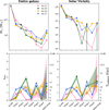 |
Fig. 1 Current (z = 0) stellar mass (upper row) and redshift of accretion (lower row) of the six most massive accreted progenitors of the four Auriga MW-like galaxies studied here. The stellar mass of the in situ component at z = 0 is also indicated for comparison, as it is the redshift of accretion of the smaller progenitors. The left column displays these properties as calculated within the entire galaxy (i.e. < R200), while the right column for the solar vicinity region (see Section 3.1). In the bottom panels, the circles (shaded regions) indicate the (range of) redshift when 50% (5–90%) of the stellar particles from a progenitor were accreted by the main galaxy. The accreted galaxies with a surviving progenitor with more than 1% of the initial mass of the progenitor at z = 0 are indicated with an open circle. |
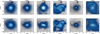 |
Fig. 2 Spatial distribution at z = 0 of the particles (accreted or still bound to the progenitor) for the six most massive progenitors (blue) compared to all particles (grey) in Au. 27. Note: the physical distances presented here have been rescaled, such as the scale-length of the simulated disc is similar to the scale-length of the MW (see Section 2.1). |
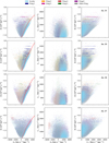 |
Fig. 3 Dominance diagrams of IoM space of the solar vicinity for the four simulated galaxies analysed. Each progenitor is identified by a specific colour, as indicated in the legend. In these diagrams, the local uniqueness of a colour indicates that the region is mainly populated by particles originating from a single progenitor. On the contrary, regions where particles have different origins are identified by areas with blended colours, proportional to the local contribution of each progenitor. The density variation is logarithmically proportional to the colour opacity. The red line on the left panels indicates the approximate limit of the kinematically selected halo (see Section 3.1). |
3 Methodology adapted to the Auriga simulations
To identify the signatures of accreted galaxies, we followed the methodology described in L22. This involves searching for overdensities that could be caused by merger debris in the IoM space using a single linkage-based clustering algorithm. The significance of these clusters is quantified by comparing them to artificially created smoothed halos.
The hypothesis behind this approach is that the debris of an accreted galaxy remain clustered in IoM space even several gigayears after the complete dissolution of the progenitor (Helmi & White 1999). It is also implicitly assumed that the gravitational potential of the host galaxy can be well approximated by a time-independent axisymmetric potential, since the employed IoMs are the total energy (E), the vertical angular momentum (Lz), and the perpendicular angular momentum (L⊥). All of these assumptions are, in reality, somewhat broken. For instance, L⊥ is not fully conserved in an axisymmetric potential. Nonetheless, it is often used in searching for signatures of accreted galaxies, as it is generally expected that stars originating from the same progenitor remain clustered for several gigayears in this parameter space (e.g. Helmi & White 1999; Williams et al. 2011; Jean-Baptiste et al. 2017; Koppelman et al. 2019b). Even regarding the other parameters, it has been shown that the quantities are not always conserved during and after the accretion, in particular for the most massive galaxies, as their energy and angular momentum decrease rapidly due to dynamical friction, which can result in several local overdensities at different energy and angular momentum level (e.g. Jean-Baptiste et al. 2017; Grand et al. 2019; Amarante et al. 2022; Khoperskov et al. 2023b). Another source of limitation of these assumptions is that the Galactic gravitational potential is not axisymmetric, due to the presence of the bar, spiral arms or large scale perturbations that affect the dynamics of disrupted structures (see Pearson et al. 2017; Vasiliev et al. 2021; Thomas et al. 2023, for the impact of non-axi-symmetries on stellar streams), and because it is varying over time (e.g. Buist & Helmi 2015; Koppelman & Helmi 2021). The algorithm from L22 used to detect substructures in the IoM space is succinctly outlined below; however, we refer to Sects. 3 and 4 of that work for a more detailed description.
The first step is based on the single linkage method (Everitt et al. 2011) to identify potential clusters in the IoM. This hierarchical clustering procedure incrementally connects the two closest groups of stars (or two individual stars) that are not yet connected according to a given metric. The metric chosen by L22 was the Euclidean distance between two (groups of) stars in the scaled IoM space. Indeed, to ensure that each IoM parameter (E, Lz, L⊥) is equally important when searching for clusters, each of them is rescaled such that the values of the distribution are in the range [−1,1].
In the second step of the algorithm, the significance of each potential cluster (Ci) found in the previous step is computed by comparing the number of stars belonging to the cluster, NCi, to the average number of stars ![Mathematical equation: $\[\langle N_{C_{i}}^{a r t}\rangle\]$](/articles/aa/full_html/2025/12/aa52449-24/aa52449-24-eq1.png) measured in the same region of the IoM space in a set of 𝒩 artificial halos, whose generation process is described in the Sect. 3.3. As done by L22, we only investigated candidate clusters with at least ten members, since smaller clusters are not significant assuming Poissonian statistics. It is important to acknowledge that this minimum threshold may restrict our ability to detect debris from low-mass accreted galaxies with stellar masses ~106 M⊙, since they are composed of ~100 stellar particles in the simulations used here. Following L22, the area covered by of each potential cluster is assumed to be elliptical, with the axis lengths equal to
measured in the same region of the IoM space in a set of 𝒩 artificial halos, whose generation process is described in the Sect. 3.3. As done by L22, we only investigated candidate clusters with at least ten members, since smaller clusters are not significant assuming Poissonian statistics. It is important to acknowledge that this minimum threshold may restrict our ability to detect debris from low-mass accreted galaxies with stellar masses ~106 M⊙, since they are composed of ~100 stellar particles in the simulations used here. Following L22, the area covered by of each potential cluster is assumed to be elliptical, with the axis lengths equal to ![Mathematical equation: $\[a_{i}=2.83 ~\sqrt{\lambda_{i}}\]$](/articles/aa/full_html/2025/12/aa52449-24/aa52449-24-eq2.png) , where λi are the eigenvalues obtained using a principal component analysis (PCA, Pearson 1901; Hotelling 1933) on stars composing the potential cluster. As L22, the clusters below a significance threshold of 3σ are discarded, such that only the clusters where
, where λi are the eigenvalues obtained using a principal component analysis (PCA, Pearson 1901; Hotelling 1933) on stars composing the potential cluster. As L22, the clusters below a significance threshold of 3σ are discarded, such that only the clusters where ![Mathematical equation: $\[N_{C_{i}}-\langle N_{C_{i}}^{a r t}\rangle \geq 3 \sigma_{i}\]$](/articles/aa/full_html/2025/12/aa52449-24/aa52449-24-eq3.png) are conserved. Here
are conserved. Here ![Mathematical equation: $\[\sigma_{i}=\sqrt{N_{C_{i}}+\left(\sigma_{C_{i}}^{a r t}\right)^{2}}\]$](/articles/aa/full_html/2025/12/aa52449-24/aa52449-24-eq4.png) , where
, where ![Mathematical equation: $\[\sigma_{C_{i}}^{a r t}\]$](/articles/aa/full_html/2025/12/aa52449-24/aa52449-24-eq5.png) is the standard deviation of the number of stars detected over the set of 𝒩 artificial halos5. Some identified clusters with at least a significance of 3σ overlapped to each other in the IoM space and are linked together by the single linkage method. Therefore, by making the assumption that the significance increases by adding stars of the same structure and decreases by adding noise, we can select the final exclusive clusters by searching the location of the maximum significance of connected significant clusters (more than 3σ). In practice, this is done by exploring the merger tree of the significant clusters obtained by the single linkage method, ordered by descending significance (see Section 4.1.2 of L22).
is the standard deviation of the number of stars detected over the set of 𝒩 artificial halos5. Some identified clusters with at least a significance of 3σ overlapped to each other in the IoM space and are linked together by the single linkage method. Therefore, by making the assumption that the significance increases by adding stars of the same structure and decreases by adding noise, we can select the final exclusive clusters by searching the location of the maximum significance of connected significant clusters (more than 3σ). In practice, this is done by exploring the merger tree of the significant clusters obtained by the single linkage method, ordered by descending significance (see Section 4.1.2 of L22).
In L22 and D23, the number of stars in each cluster was refined by retaining only those with a Mahalanobis distance from the cluster centre of less than 2.13. This approach preserves 80% of the original cluster members, assuming the stars in a cluster follow a multivariate Gaussian distribution in the IoM. Furthermore, they include extra members by adding all stars located within that Mahalanobis distance range, even if they were not part of the original clusters according to the single linkage method. However, we found that this revised selection has a minimum impact on our results (see discussion about it in Sect. 4.1). Therefore, we decided to keep the original cluster populations, without adding extra members.
The steps outlined above are solely based on the stars’ IoM properties. In a companion article, RL22 also investigated whether incorporating additional information about the stellar population properties, such as the average age and metallicity distribution function (MDF), could provide further insight into the reality of these features. In Sects. 4.2 and 4.4, we explore this approach as well.
3.1 Selection of the halo sample in the solar vicinity
Akin to what has been done in several works to identify the local stellar halo of the MW in data (Koppelman et al. 2018, 2019b; Lövdal et al. 2022; Dodd et al. 2023), we selected particles with halo-like kinematics, requiring them to have a total velocity with respect to the local standard of rest (LSR; VT ≡ |V − VLSR|) above a given threshold velocity (Vth), chosen to remove the large majority of the particles of the galactic disc.
In the simulations, VLSR is equal to the circular velocity at the solar radius Vcirc(R⊙). For each simulated galaxy, we obtain the circular velocity curve (presented in Fig. 5) from young (≤1 Gyr old) in situ stellar particles located within 1 kpc of the Galactic plane. The circular velocity at the solar radius is Vcirc(R⊙) = 229.5 km s−1 for simulation Au. 21, 261.4 km s−1 for Au. 23, 207.2 km s−1 for Au.24 and 261.1 km s−1 for Au.27.
Ideally, we would like to fix the threshold velocity (Vth) used to select the stellar halo, so that the majority of the particles with VT ≥ Vth originated from accreted galaxies. However, as visible in Fig. 6, this is not possible in all simulations, as the fraction of accreted stars remains at most of 45–55% even for Vth = 350 km s−1, at which point the completeness would drop to 10–25%. Therefore, we decided to use the same threshold velocity than Koppelman et al. (2018, 2019b) and L22 (i.e. Vth = 210 km s−1) since it yields a fraction of accreted stellar particles not too dissimilar than when adopting larger thresholds, but for a much higher level of completeness.
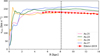 |
Fig. 5 Circular velocity curve of the four MW-like galaxies studied here. We note that the radii have been rescaled as explained in Section 2.1. The solar radius (R⊙ = 8.2 kpc) is indicated by the black vertical line. For comparison, we show the rotation curve of the MW measured by Eilers et al. (2019). |
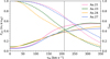 |
Fig. 6 Fraction of accreted stellar particles (ℱacc, solid lines) in the solar vicinity with velocities above a given threshold velocity (Vth), for the four simulated galaxies. The dashed lines show the evolution of the completeness of accreted stellar particles (𝒞acc) as a function of the threshold velocity. The vertical dashed line indicates a velocity threshold of 210 km s−1, used to kinematically define the halo in the solar vicinity. |
3.2 Calculation of IoM and re-normalisation in IoM space
We computed the total energy of each particle using directly the gravitation potential of the simulated system. In our case, the factors used to re-normalise the distribution of E, Lz, and L⊥ are different for each simulated galaxy, given that they cover a different range of the parameter space. The values used to re-normalise the IoM space for each galaxy, listed in Table 1, correspond to the approximate minimum and maximum range spanned by each of these parameters for the stellar particles in the solar vicinity. The re-normalised parameters space of the local halo sample of each simulated galaxy is compared to that of the L22 sample given in Fig. 7. In this figure, we can see that, with the notable exception of Au. 23, which has a clear overdensity of particles with high vertical angular momentum, all the simulated systems have a distribution in the re-normalised IoM space similar to that observed in the MW solar neighbourhood. However, we can also see that none of them present a structure similar to the GES in the energy-vertical angular momentum plane, which in the data is clearly visible by the almost vertical overdensity around (Lz,scaled, Escaled) = (0, 0). This is very interesting, as Fattahi et al. (2019) found that Au. 24 and Au. 27 have a progenitor with current characteristic similar to the GES. However, their criteria, based on the velocity anisotropy, and the region (9 < |z| < 15 kpc) used to identify this progenitor, are different from the criteria we used and the region we study. Orkney et al. (2022) also identified a GES-like progenitor in Au. 24, which was chosen to have a redshift of accretion and a stellar mass similar to the estimation obtained for GES (z ≃ 2–1.5, M* ~ 108−109 M⊙, Helmi et al. 2018; Mackereth et al. 2019; Gallart et al. 2019; Naidu et al. 2022; Lane et al. 2023). Their GES-like progenitor corresponds to our Prog. 2 of Au. 24, and their Kraken-like progenitor corresponds to Prog. 3. In their Fig. 3, we can see that the GES structure presents a vertical profile centred on Lz = 0 km s−1 kpc−1. However, the region they are studying is larger than the volume of the solar vicinity we are using in this study, which naturally tends to increase the energy it spans, and the scattering in Lz is significantly larger than the actual scatter of GES.
Boundary of each IoM parameter used to rescale their distribution into the range [−1,1] for the dynamically selected halo.
3.3 Generation of the artificial halos
As mentioned in a previous section, the significance of each cluster is computed by comparing the number of particles inside an IoM region to that in a set of 𝒩 artificial halo. Similar to L22, the artificial halos are made by scrambling two of the three the velocity components of the original dataset (i.e. in practice vy and vz). By doing so, these artificial halos are smoother than the original dataset, since the structures present in the integral-of-motion space are washed out (Helmi et al. 2017). However, by scrambling the velocities, this method tends to increase the kinetic energy of individual stars and, thus, their total energy. As a result, some stars with a high potential energy might end up having a positive total energy in these artificial halos; thus, they would no longer be bound to the galaxy.
To mitigate this problem, L22 generated the artificial halos by scrambling the velocity of an extended halo sample, selected using a less restrictive kinematic criterion of Vth,art = 180 km s−1, instead of Vth = 210 km s−1 for the original halo sample. The artificial halo is then obtained by sub-selecting N stars with VT ≥ 210 km s−1 from this extended halo sample, where N is the number of stars present in the original halo dataset.
In our case, because the distribution in the IoM space is very different across the simulated galaxies to another, it is not possible to use a unique value of Vth,art. Our experiments revealed that using a common value of Vth,art for all the simulation led to notable discrepancies between the artificial halos and their corresponding original counterparts. In particular, the artificial halos consistently exhibited higher average vertical angular momentum than the original halos.
To determine the optimal Vth,art for each case, we conducted a systematic analysis where we calculated the average values of IoM parameters (E, Lz, and L⊥) across ten artificial halos for various Vth,art values, ranging from 50 to 210 km s−1 with an increment of 5 km s−1. The correct Vth,art value was identified as the one at which the normalised Euclidean distance (D) between the means of IoM parameters in the original halo dataset and those in the set of ten artificial halos was minimised. Mathematically, this is expressed as
![Mathematical equation: $\[D=\sqrt{\sum_{X=E, L_z, L_{\perp}}\left(\frac{\left\langle X_{a r t}\right\rangle-\left\langle X_{o r i}\right\rangle}{\sigma_{X, o r i}}\right)^2},\]$](/articles/aa/full_html/2025/12/aa52449-24/aa52449-24-eq6.png) (1)
(1)
where σX,ori is the standard dispersion of each IoM parameters in the original halo.
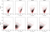 |
Fig. 7 Distribution of the rescaled IoM parameters of the kinematically selected local halo sample of the four simulated galaxies (black contours). As a comparison, in each panel, the distribution of the local MW halo sample by L22 is shown by the red contours. In both cases the iso-density contours are plotted at the 1, 10, 20, 50, and 90% of the maximum density. |
4 Analysis and results
We applied the methodology described in Sect. 3 to the four Auriga halos previously discussed. In the remainder of the article, we use Au. 27 to discuss some of the results in context because this halo presents an accretion history that is the closely resembles the one currently estimated for the MW. Specifically, it is characterised by two important accretion episodes occurring at z ≃ 1–2 (see Deason & Belokurov 2024, and references therein for a recent review on the vision of the MW history), similarly to GES and Kraken, as well as one more important accretion in the last 4–6 Gyr. For this latter episode, the debris of the progenitor is still forming a stellar stream at z = 0, similarly to the Sagittarius stream in the MW. The results and plots concerning the other halos are included as online material.
Table B.1 lists the statistically significant clumps found for Au. 27, along with their main properties (number of particles, significance, fraction of particles accreted, mean position in the IoM, dominant progenitor, contribution of the dominant progenitor to the cluster), as well as their suggested association in groups on the basis of a threshold in Mahalanobian distance in IoM space between the clusters (see Sect. 4.3) and with the addition of the information on the metallicity, magnesium abundance, and age distribution of the stellar particles belonging to them. We find 63 clusters, with statistical significance between 3 and 17 and containing from a few dozen up to more than 4000 particles, with a median of 58 particles per cluster. These values are similar to those encountered by L22. This indicates that the kinematically selected stellar halo of Au. 27 presents a similar level of lumpiness as observed in the MW. The fraction of stellar particles that are associated with clusters is ~9.4%, similar to the values found by L22 and D23 for the MW (~13%). In the other simulated galaxies, the number of significant clusters found ranges from 49 (Au. 24) to 111 (Au. 23), with a fraction of stars in clusters varying from 4% (Au. 24) to 13.5% (Au. 23), reflecting the different accretion histories that occur in each of them. We go on to examine the general purity and recovery rate (completeness) both of the individual clumps and then of the groups themselves.
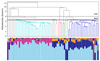 |
Fig. 8 Dendrogram (similar to Fig. 10 of L22) showing the relationship between the significant clusters detected by the single linkage algorithm according to their Mahalanobis distance in the IoM space, with the same cut-off threshold as used by D23 (indicated by the black line). For reference, the cut-off threshold used by L22 is shown by the dashed line. The vertical bars at the bottom of the figure indicate the relative contribution of the different progenitors to each significant cluster, using the same colour scheme as in Fig. 3. Note: the colours used to indicate the different groups of clusters linked together in the dendrogram are not related to the progenitors. |
4.1 Recovery rate and purity of individual clumps
The bottom panel of Figure 8 displays, for each of the individual statistically significant clumps, their composition in terms of birth environment and progenitor, with the length of the vertical bars being directly proportional to the percentage of particles belonging to that progenitor (the most dominant progenitor is found at the bottom of the bar). Across all halos, the majority of clumps are heavily contaminated by the presence of in situ particles, with the exact percentage varying from halo to halo. In Au. 27, and this is particularly the case for this simulation, in situ particles are numerically dominant in all but a minority of clumps. This is a surprising result, as in situ particles are not expected to form overdensities, unlike accreted particles. Some of these in situ dominated clusters might have originated from the response of the Galactic disc to past mergers (Gómez et al. 2012; Jean-Baptiste et al. 2017; Laporte et al. 2018a; Thomas et al. 2019), but this will explain the presence of such clusters on prograde orbits. However, we found that between 20 and 40% of clusters where in situ particles make up more than 50% of the population are located at Lz < 500 km s−1 kpc−1.
Moreover, it is also rare to find clumps where all the (or at least the great majority of) particles originate from a single accreted progenitor, except for possible cases of in situ particles formed from gas that was previously bound to accreted galaxies. For instance, in Au. 21 (23), only 5 (17) out of 54 (111) clusters have more than 75% of their particles originating from a single accreted progenitor, with just one such cluster in both Au. 24 and Au. 27. This number further drops to 2 (5) clusters in Au. 21 (23) and none in Au. 24 and Au. 27 when the threshold is increased to 90%. Similar results were obtained by wu et al. (2022), who analysed the substructures identified by Enlink on MW-like galaxies from the FIRE-2 suite of simulations.
None of the simulations show a clear trend between the purity (i.e. the relative contribution of the dominant progenitor) and the significance of a cluster, regardless of the inclusion or not of in situ particles. However, for significance higher than 7–8, we observe that the minimum purity of the clusters is of ≃0.6, which increases such that clusters with a significance >15 are pure at 90%. This remains true even when the clusters are separated into different categories based on their population size. This is surprising because it is reasonable to expect that the most significant clusters would be mainly composed of particles from a single progenitor, since these clusters are much more populated compared to a smooth background. This lack of correlation between the purity and the significance indicates a limitation of the method, and might be linked to spurious overand under-densities from the generation of artificial backgrounds (see Sect. 5).
Figure 9 shows that the rate of recovering accreted particles as part of statistically significant clumps is in general below 10–15%. This percentage drops to <5% if we count only particles belonging to the dominant progenitor of a given clump6. Exceptions to this behaviour are progenitor 3 in Au. 21, progenitor 1 in Au. 23, 1–4–5 in Au. 24 (only 5 for the case of the dominant particles), progenitor 4 in Au. 27; qualitatively speaking, these are essentially those progenitors that produce the tight clumpy features in energy visible in Fig. 3, i.e. typically those that have been recently accreted (z < 0.6; < 6 Gyr ago), and are found either in a stream- or disk-like configuration and do contribute with a sufficient percentage of particles to the sample in the volume being analysed. In the four simulations, all the clusters with a significance higher than 6σ not dominated by in situ particles are dominated by particles originating by a galaxy accreted less than 6–7 Gyr ago. Interestingly, this relationship between the recovery rate and the age of accretion is independent of the total or stellar mass involved in the merger. Although all these recent accretion events are minor mergers, with a stellar mass ratio of less than 10:1, their impact on the recovery rate appears negligible, provided the progenitors leave debris in the solar vicinity. This result is intriguing because, for a given accretion time, we might expect the debris of smaller progenitors to be more easily detectable, and thus having a higher recovery rate than most massive progenitors for which dynamical friction is more important, leading to a wider dispersion of debris in Integral of Motion (IoM) space (Jean-Baptiste et al. 2017) and, consequently, to a lower recovery rate.
As mentioned in Sect. 3, in L22 and D23, the number of stars assigned to a cluster is revised by selecting all stars within a Mahalanobis distance of 2.13 from the cluster centre, even if they were not part of the core selection made by the single linkage method, and by excluding all stars beyond this distance. Applying the same method to our simulations, we found that the fraction of stars increased of order 1%. The revised selection had a negligible impact on the purity of clusters; however, the recovery rate worsened, particularly when considering only the particles belonging to a progenitor that dominates a given clump. For example, the recovery fraction for Prog. 3 in Au. 21 dropped from 66% to 58%, for Prog. 5 in Au. 24 it dropped from 29% to 26%, and for Prog. 4 in Au. 27 it dropped from 73% to 65%. Notably, clusters dominated by these progenitors display the highest level of purity. For the other progenitors, the recovery fraction was similar between the two cases. Given the negligible impact of the revised selection on our results and conclusions, we retain the initial selection obtained by the single linkage method for the rest of the paper.
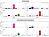 |
Fig. 9 Percentage of stellar particles, separated by their birth environment, located in the kinematically selected halo in the solar vicinity identified as being part of any significant cluster (>3σ) by the single-linkage method (upper panels). The lower panels show the similar quantity but considering only the particles that belong to clusters where their progenitor is the dominant contributor to a given clump. In all panels, the grey histograms indicate the contribution of each progenitor to the solar vicinity halo. Note: the second bar represent the value of all the accreted stellar particles grouped together. |
4.2 Chemical and age properties of the individual clumps
Although, the single linkage method only uses dynamical properties to detect the clusters, chemical and stellar age information can be used in disentangling clusters (or structures) dominated by accreted particles from those mostly populated by stars formed in situ (e.g. Nissen & Schuster 2010; Kruijssen et al. 2020; Gallart et al. 2019; Belokurov & Kravtsov 2022; Bellazzini et al. 2023; Dodd et al. 2023). In Fig. 10, we show the median [Fe/H], [Mg/Fe], and stellar age of the cluster populations as function of their average vertical angular momentum, colour-coded by the fraction of accreted particles they contain. We separated the clusters in three main orbital categories: retrograde (Lz < −500 km s−1 kpc−1), non-rotating (−500 < Lz < 500 km s−1 kpc−1), and prograde (Lz > 500 km s−1 kpc−1). In all the simulations, the large majority of clusters that are predominantly composed of in situ particles (ℱacc < 0.3) are prograde. Although, as mentioned in the previous section, the detection of such a high number of clusters dominated by in situ particles is unexpected, it is not surprising that such clusters are prograde. This is consistent with the fact that in the solar vicinity, 50–70% of the prograde kinematically selected stellar halo is populated by in situ particles, and that 40 to 60% of the in situ particles of the stellar halo are on prograde orbits, except for Au. 24, where this percentage drops to 29%, as shown in Fig. 3.
However, some clusters dominated by in situ particles are also encountered on non-rotating and on retrograde orbits. The presence of in situ dominated clusters in the non-rotating region is not unexpected, as in the MW it has be shown that up to ≃50% of the halo stars with a low circularity can be born in situ (Bonaca et al. 2017; Haywood et al. 2018; Di Matteo et al. 2019; Amarante et al. 2020), either because they were formed in the proto-galaxy (also called Aurora; Belokurov & Kravtsov 2022; Chandra et al. 2023), or because they were part of the disc and were subsequently splashed into halo orbits due to an interaction with a massive progenitor (Di Matteo et al. 2019; Gallart et al. 2019; Belokurov et al. 2020). What is more surprising is the observation that in situ particles can also dominate a significant fraction of retrograde clusters (≥60%, except for Au. 23), with a contribution of in situ particles to the cluster in the order of 50–60%, and in some cases reaching up to ≃90% in Au. 21. This is unexpected, given that the retrograde halo is generally thought to be largely populated by accreted stars (Naidu et al. 2020; Myeong et al. 2022; Horta et al. 2023; Ceccarelli et al. 2024).
From Fig. 10, we can see that prograde clusters dominated by in situ particles tend to be more metal-rich by approximately 0.3 dex compared to those dominated by accreted particles. However, in [Fe/H], some clusters dominated by accreted particles overlap with clusters mostly populated by in situ particles. When the contribution of in situ stars to the clusters’ properties is excluded, as indicated by the black triangles, the median metallicity of prograde clusters generally tends to be lower and more widely distributed. However, some clusters still exhibit a relatively high metallicity ([Fe/H] ≃ −0.6 dex), similar to when in situ particles are accounted for, even for well-populated clusters (>100 particles), particularly in Au. 23 and Au. 27. On the other hand, [Mg/Fe] and stellar age provide a clearer distinction between prograde clusters dominated by accreted particles and those dominated by in situ particles, with the former ones being ~0.05–0.1 dex richer in [Mg/Fe] and ~4 Gyr older than the latter. This distinction is further confirmed by the median values of these quantities when in situ particles are removed from prograde clusters, as the median [Mg/Fe] and stellar age accounting only for accreted particles closely resemble those of clusters that are actually dominated by accreted particles.
Regarding the non-rotating and retrograde clusters, none of the studied parameters can effectively distinguish between clusters dominated by accreted particles and those dominated by in situ particles. Indeed, regardless of the galactic origin of the dominant populations, the clusters are populated by old (~10–12 Gyr) metal-poor ([Fe/H] < −1.0) and alpha-rich ([Mg/Fe] ≃ 0.2) particles. Even when in situ particles are not taken into account, the properties of the non-prograde clusters remain similar. This is in line with the results of Khoperskov et al. (2023a), who find that in situ particles without net rotation and on retrograde orbit have a similar mean metallicity than the accreted particles, while prograde in situ particles are ~0.5 dex more metal-rich than accreted one on similar orbits. However, none of the detected clusters dominated by in situ particles have a median metallicity lower than [Fe/H] < −1.35. Although the statistics are limited, this allows us to tentatively suggest that clusters with a median metallicity lower than [Fe/H] < −1.35 are dominated by accreted particles, while the origin of the dominant population for clusters above this threshold remains unclear. Nevertheless, it is important to stress that the majority of clusters with a high fraction of accreted particles have a median metallicity [Fe/H] > −1.4. As such, this criterion does not allow for the detection of all the debris left by accreted galaxies.
It is not entirely possible to exclude the possibility that some of the particles classified as in situ are actually formed in the gas clouds brought by an accreted galaxy, in particular for those on non-rotating or retrograde orbits (e.g. Pillepich et al. 2015). If it is the case, this might explain why the fraction of in situ particles on retrograde orbits (~50%) is higher than found in other simulations (e.g. Khoperskov et al. 2023a), but also why the clusters detected on these orbits share the same properties, regardless of the fraction of accreted particles they contain. However, it seems unlikely that this is the only explanation, as the high fraction of in situ particles found in clusters would require that 40–70% of the stars originally from an accreted event were formed during or shortly after the accretion process.
It is interesting to compare the chemical characteristics of the clusters’ populations with the fraction of accreted particles measured in the [Fe/H]-[Mg/Fe] plane for different orbital properties, as shown in Fig. 11. With the notable exception of Au. 24, the relative fraction of accreted stars remains largely unchanged across different orbital properties. in situ particles dominate the low-alpha region, while accreted particles dominate the high-alpha region, and [Fe/H] ≲ −1.4, regardless of [Mg/Fe] value. This last point supports our hypothesis that clusters with median metallicity below this threshold are dominated by accreted particles, regardless of its orbital properties. At higher metallicities, a clear separation emerges between in situ and accreted particles based on [Mg/Fe]. However, the contour lines representing the particle distribution indicate that, that except for the prograde region, the vast majority of the particles have chemical properties where both accreted and in situ population coexist, with typically an accreted fraction of ~0.3. This explains why the chemical properties of retrograde and non-rotating clusters are similar, regardless of the origin of their population.
It is also interesting to note that prograde in situ particle reach a higher metallicity than that on retrograde and non-orbiting orbit. Accreted particles do not necessarily exhibit such behaviour, as the most metal-rich stars tend to originate from one or two accreted progenitors. These progenitors can have varying orbital properties from one galaxy to another, reflecting the diverse formation histories of these galaxies. This is very interesting as Kordopatis et al. (2020) found super-solar metallicity stars on retrograde orbits in the MW. In addition, the simulations seem to suggest that these stars could have an accreted origin.
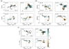 |
Fig. 10 Median [Fe/H] (panels a), [Mg/Fe] (panels b), and stellar age (panels c) as a function of the mean (Lz) of each cluster found in the kinematically selected halo of the solar vicinity in the four simulated galaxies (circles). The circles are colour-coded by their fraction of accreted stellar particles. The triangles represent the same quantity, but with the in situ particles removed. The vertical dashed lines located at (Lz ± 500 km s−1 kpc−1) indicate the separations between the retrograde, non-rotating, and prograde clusters. For the prograde clusters, the metallicity, but mostly the [Mg/Fe] and the stellar age separate well those dominated by in situ and accreted particles. However, none of those parameters is able to disentangle the clusters dominated by in situ to those dominated by accreted particles for the non-rotating and the retrograde clusters. |
4.3 Association of clumps into groups
As discussed in L22 and RL22, the fact that the single linkage method finds an individual cluster does not necessary mean that it is a unique structure by itself, because a single accreted galaxy can generate several clusters/over-densities in the IoM space (Gómez et al. 2013; Jean-Baptiste et al. 2017; Grand et al. 2019; Koppelman et al. 2020; Khoperskov et al. 2023b; Mori et al. 2024). In that sense, L22 tentatively proposed that neighbouring clusters in dynamical space might be populated by the same progenitor. As the volume occupied by each cluster is different, these authors used the Mahalanobis distance between two clusters as a metric to find group of nearby clusters,
![Mathematical equation: $\[\mathrm{D}_{\mathrm{M}}=\sqrt{\left(\boldsymbol{\mu_1}-\boldsymbol{\mu_2}\right)^T\left(\Sigma_1+\Sigma_2\right)^{-1}\left(\boldsymbol{\mu_1}-\boldsymbol{\mu_2}\right)},\]$](/articles/aa/full_html/2025/12/aa52449-24/aa52449-24-eq7.png) (2)
(2)
where μi and Σi describe the mean and the covariance matrix of the i-th cluster, respectively. The Mahalanobis distance between two clusters is then used by a single linkage method to generate a dendrogram as shown on the top panel of Fig. 8 (for Au. 27; the same figures for the other halos are available online). The individual clumps are associated in groups according to a Mahalanobis distance cut-off value. We colour-coded those that are associated with each other adopting the same cut-off as D23.
In Au. 27, there are five groups of clumps associated with each other, with group sizes ranging from 2 to 25 clusters. This is similar to the number of groups found by L22 and D23 in the MW. Additionally, 10 clusters are not associated with any group because they are too distant from other clusters in the IoM space. This is clearly visible in Fig. 12, which shows the locations of these different groups in the IoM space of Au. 27.
The dendrogram of Fig. 8 shows that clumps for which the most dominant accreted progenitor is Prog. 1 (in blue) or Prog. 3 (in pink) tend to be grouped together. However, there is no strict one-to-one correspondence between a single group and a single main accreted progenitor. Moreover, we can see that some clusters with different dominant accreted progenitors are grouped together. For instance, cluster 61, which is well-populated (Npart ≃ 380) and dominated by Prog. 4 (red), is linked to a group that is mostly dominated by particles formed in situ and in Prog. 1 (see Table B.1).
It is clear from that figure that the cluster associations are highly sensitive to the Mahalanobis distances threshold used to group clusters together. For example, a threshold slightly lower than the one used by D23 would prevent cluster 61 from being linked to most of the clusters dominated by Prog. 1. On the contrary, using the same threshold as L22 will result in more clusters dominated by different accreted progenitors being grouped together. While the specifics vary from halo to halo, this general trend remains consistent across the different simulated galaxies. Therefore, a natural question arises: is there a Mahalanobis distance threshold that can maximise the number of clusters dominated by the same progenitor grouped together without incorporating clusters dominated by other progenitors? In other words, can we optimise both the completeness of clusters dominated by the same progenitor linked into the same group, and the purity of each group of clusters? Given the predominance of in situ contaminants, and they are not expected to be clustered in IoM space, we do not account for in situ particles in the following calculations7.
We define the completeness as the fraction of pairs of significant clusters dominated by the same progenitor that are grouped together. Mathematically, for a given Mahalanobis distances threshold (DM,th) this is expressed as
![Mathematical equation: $\[\mathcal{C}\left(\mathrm{D}_{\mathrm{M}, \mathrm{th}}\right)=\sum_p \frac{2}{C_p\left(C_p-1\right)} \sum_{\substack{i, j=1 \\ i \neq j}}^{C_p} \delta\left(G_i, G_j\right),\]$](/articles/aa/full_html/2025/12/aa52449-24/aa52449-24-eq8.png) (3)
(3)
where p represents a given dominant progenitor, Cp is the number of clusters dominated by this progenitor, and Gi is the ID of the group to which belong the cluster i. The evolution of the completeness of the four simulations studied here as function of the adopted Mahalanobis distance threshold is presented in the left panel of Fig. 13. We see that for Au. 24 and Au. 27, the completeness rises rapidly, reaching a plateau of 0.7 between 3.5 < DM,th < 7.0. On the contrary, for Au. 21 and Au.23, the completeness is below 0.2 up to DM,th ≃4–5, and then rises suddenly to unity. Several factors can explain the difference observed between the different simulations. For Au. 24, the quick rise of the completeness is explained by the fact that five different progenitors dominate the different clusters, which are furthermore relatively close one to another. Therefore, the distance threshold needed to regroup together most of the clusters dominated by the same progenitor is relatively low. For Au. 23, the slow rise of the completeness is a consequence of the large spread in the IoM of Prog. 1 which is highly clustered at different energy levels (see Fig. 4). Therefore, a higher distance threshold is needed to link most of them into the same group. The reasons behind the difference between Au. 21 and Au. 27 are less clear. A tentative explanation is that in Au.27 the two progenitors that dominate the IoM (Prog. 1 and 3; see Fig. 4) occupy two different regions in the IoM space, while at the same time, for Au. 21, the separation between Prog. 1 and 2 is less clear, as they overlap in energy and perpendicular angular momentum. From these results, we observe that with the Mahalanobis distance threshold adopted by D23, on average, between 11% and 56% of the clusters dominated by the same progenitor are grouped together. With the less restrictive threshold adopted by L22, these values increase to 15% and 68%. Based on these results, it is likely that several different groups found by L22 and D23, which are assumed to be populated by different accreted galaxies, are actually formed by the same single progenitor.
Regarding the purity, several definitions are imaginable. For instance, it is possible to define the purity as the relative contribution of the dominant progenitor of the group in terms of mass fraction (or fraction of particles). In that case, the purity is largely dominated by the most populated cluster of the group, which often is an order of magnitude more populated than the other clusters. As a result, with this definition, the purity does not change significantly with the Mahalanobis distance threshold adopted. Although this definition of the purity is valid, its use in determining the optimal threshold value is limited. An alternative and potentially more insightful definition of the purity is to consider it as the fraction of clusters within a given group that are dominated by the most common dominant progenitor in that group, averaged over the different groups. In other words, with this definition, the purity corresponds to the average fraction of clusters grouped together that are dominated by the same progenitor. Mathematically, this can be expressed as
![Mathematical equation: $\[\mathcal{P}_{c g}\left(\mathrm{D}_{\mathrm{M}, \mathrm{th}}\right)=\frac{1}{\mathrm{G}\left(\mathrm{D}_{\mathrm{M}, \mathrm{th}}\right)} \sum_{g=1}^{\mathrm{G}}\left(\frac{1}{C_g} \sum_{i=1}^{C_g} \delta\left(P_{g i}, P_{g, m o s t}\right)\right),\]$](/articles/aa/full_html/2025/12/aa52449-24/aa52449-24-eq9.png) (4)
(4)
where G(DM,th) is the number of groups for a given Mahalanobis distance threshold value (DM,th), Cg is the number of clusters belonging to the group, g, and Pgi is the dominant progenitor of the cluster, i, of the group, g. The term Pg,most represents the most common progenitor in a group g, defined as
![Mathematical equation: $\[P_{g, m o s t}=\operatorname{argmax}_P\left(\sum_{i=1}^{C_g} \delta\left(P_{g i}, P\right)\right).\]$](/articles/aa/full_html/2025/12/aa52449-24/aa52449-24-eq10.png) (5)
(5)
We note that in the case of several equally dominant progenitors, we randomly selected one of the progenitors, since the result of Eq. (4) is invariant to the choice of the dominant cluster in Eq. (5). With this definition, when lim DM,cut → ∞, the purity reaches a plateau that corresponds to the fraction of clusters that are dominated by the same progenitor (i.e. the dominant progenitor the most encounter across all the clusters). As we can see from the plain lines in the right panel of Fig. 13, we observe that the most frequent dominant progenitor tends to dominate 60% of the overall clusters found in the halo of the solar vicinity, except for Au. 24, where it dominates only 30% of the clusters. The reason for this is that in the other galaxies, two progenitors dominate 80% of the clusters, while in Au. 24, the number of dominant progenitors is higher. It is also noticeable that, with this definition, the evolution of the purity is not monotonic, and can increase when DM,th increases. Although this might seem counter-intuitive, it highlights the fact that two groups of different sizes dominated by the same progenitor can be joined together, which in some cases can increase the purity. Using this definition, we see that the purity is relatively similar for both Mahalanobis distance threshold adopted by L22 (𝒫cg ≃ 0.94) and by D23 (𝒫cg ≃ 0.97). This mean that, respectively, on average, only 6% and 3% of the clusters of a group have a different dominating progenitor than the other clusters of the group. However, this number has to be taken with care, as at low DM,th, the large majority of the group are composed of 2 or 3 clusters, which can bias the results. Instead, we find that the purity is above 0.9 for groups composed of maximum four clusters, and decrease to 0.6–0.7 for group of six or more clusters.
Another interesting way to define the purity is to wonder what is the probability that a group is entirely composed of clusters dominated by the same progenitor. It is mathematically defined as
![Mathematical equation: $\[\mathcal{P}_g\left(\mathrm{D}_{\mathrm{M}, \mathrm{cut}}\right)=\frac{1}{\mathrm{~N}_{\mathrm{c}}} \sum_{g=1}^{\mathrm{G}\left(\mathrm{D}_{\mathrm{M}, \mathrm{cut}}\right)} \sum_{i=1}^{\mathrm{C}_g} \delta\left(P_{g 1}, \ldots, P_{g i}\right),\]$](/articles/aa/full_html/2025/12/aa52449-24/aa52449-24-eq11.png) (6)
(6)
where G(DM,cut) is the number of groups for a given Mahalanobis distances cut-off value (DM,cut), Cg is the number of clusters belonging to the group g, Pgi is the dominant progenitor of the cluster i of group g. The evolution of the purity using that definition as a function of the adopted Mahalanobis distance threshold is shown by the dashed lines in Fig. 13. With this definition, the purity is a monotonically decreasing function that varies from 𝒫g (lim DM,cut → 0) = 1 to 𝒫g (lim DM,cut → ∞) = 0. In that case, the evolution of the purity vary strongly from galaxy to galaxy, with a relatively similar bimodality, likely caused by the same reasons, as seen as with the completeness, with Au. 21 and Au. 23 having a different trend than Au. 24 and Au. 27. Adopting a threshold similar to D23, we see that typically between 40 and 60% of the groups are entirely composed of clusters dominated by the same progenitor, while with the threshold used by L22 this fraction can decrease significantly: to ~15% for halos Au. 24 and Au. 27.
In conclusion, it is challenging to determine an optimal Mahalanobis distance threshold that can simultaneously optimise both the purity and completeness of the groups of clusters. This difficulty arises from the significant variation in the results obtained from galaxy to galaxy, which reflects the diversity of their accretion histories and of the properties of their accreted galaxies. Nevertheless, following the assumption we already presented that Au. 27 is the simulations with the closest properties to the MW, it seems that a threshold close to the value adopted by D23 of DM,cut = 3.3 is well suited. Indeed, in that case, the average purity of the clusters in groups (𝒫cg = 0.97) and the purity of the groups themselves (𝒫g = 0.62) is relatively high, with a completeness of 57%8. A higher value, such as that adopted by L22 will lead to a slightly higher completeness, but decrease the purity of the group by more than a factor of 6. RL22 suggested that the MDF and the colour distribution could be used to increase the purity of the groups by identifying outliers. This approach could also improve the completeness by linking clusters with different dynamical properties but similar metallicity distributions, as could be the case for their Cl.62 that has a similar MDF to Thamnos 1 and 2, despite its locus in a different region of IoM space. We applied a similar method to the MDF and the age distribution function (ADF), but we did not observe any improvements with respect to either the purity, nor the completeness. This lack of improvement may be attributed to the high contribution of in situ particles within the detected clusters, and potentially to the misclassification of in situ particles that originated from accreted gas clouds. Consequently, we chose not to explore this method further at this stage and will defer its analysis to the following section, where we focus on a sample composed solely of accreted particles.
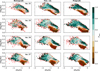 |
Fig. 11 Fraction of accreted stellar particles in different area of the [Fe/H] vs [Mg/Fe] diagram for the retrograde, non-rotating, and prograde particles of the kinematically selected halo in the solar vicinity of the four simulated galaxies. In each panel, the red contour lines show the distribution of the 1, 25, 50, 75, and 90% distribution of the particles. |
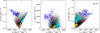 |
Fig. 12 Location in the IoM space of the grouped of clusters found in the kinematically selected halo in the solar vicinity of Au. 27 using the Mahalanobis distances. The colour scheme used is the same as for Fig. 8. The clusters that are not part of any group are shown in black. The background grey scale shows the density variation. |
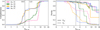 |
Fig. 13 Completeness and purity of the groups of clusters as a function of the Mahalanobis distance threshold (DM,th) chosen to group clusters together. For the purity, the solid lines represent the purity defined as the average cluster purity within groups (𝒫cg), while the dashed lines indicate the average purity of the groups (𝒫g). The threshold values used by L22 and D23 are indicated by the vertical dashed and solid lines, respectively. Note that the completeness and purity reported here only refer to the accreted progenitor. Stellar particles formed in situ are excluded (see Sect. 4.3). |
4.4 Analysis of a pure sample of accreted particles
In the above analysis, we have seen that the in situ component often dominates the budget of particles that belong to statistically significant clusters. In this section, we apply our methods to a accreted particles only9. This scenario is, of course, optimistic, as even the most advanced methods proposed in the literature for separating in situ and accreted stars in observed samples do not achieve 100% purity and completeness. For example, chemistry such as [Al/Fe] and [Mg/Mn] may not be sufficient to disentangle accreted and in situ stars with [Fe/H] < −1.3, despite the relatively successful separation for more metal-rich stars (Hawkins et al. 2015; Belokurov & Kravtsov 2022; Das et al. 2020; Horta et al. 2021; Fernandes et al. 2023).
4.4.1 Properties of the significant clusters
With the notable exception of Au. 24, the number of clusters found without the inclusion of the in situ particles is usually between 50 and 60% lower in the same IoM region than previously. Interestingly, across the different galaxies, this ratio does not change significantly between the retrograde, non-rotating and prograde regions. This confirms the important role played by the in situ particles in the clusters’ detection, as we discuss in Section 4.1.
Interestingly, we note that even when the in situ particles are removed, none of the clusters are perfectly pure, as there is always some overlap between different progenitors. However, the contamination is relatively low, as on average the dominant progenitor contributes to 70 to 80% of the particles of a cluster. However, as with the inclusion of in situ particles, we do not observe a strong dependence between the purity and significance of the clusters, nor with the number of particles that belong to a cluster.
Figure 14 shows that the recovery rate of individual progenitors is in general higher after excluding in situ stars. In particular, when considering only the particles belonging to clusters where their progenitor is the dominant contributor (bottom panel), some progenitors whose recovery fraction was very low in the in situ + accreted case now become much more prominent. This is particularly the case for the progenitor that contribute the most to the stellar halo in the solar vicinity and/or to the prograde region (for example, Prog. 1 in Au. 21, Prog. 1 in Au. 24, and Prog. 3 in Au. 27). In addition, the percentage of particles proceeding from smaller progenitors that are picked up as part of clusters also increases. This is not surprising as in situ stars are smearing some of the clumpy features out.
Even in the best case scenario of dealing with accreted particles only, for most of the progenitors, only a minority of particles are found to reside in statistically significant clusters. As for the case when in situ particles are included, the progenitors with the higher recovery rates are those that have been most recently accreted (<6 Gyr ago), as they are the most clumpy in IoM space (see Fig. 4). This essentially implies that a complete census of stars belonging to a given progenitor is hard to obtain with this methodology, even in the very favourable case of an unbiased target selection, only limited in volume. Furthermore, our simulations do not include uncertainties in distances, proper motions and radial velocities, whose effect would clearly blur the picture even more by decreasing the significance of the clusters and increasing the contamination fraction (see e.g. Helmi & de Zeeuw 2000).
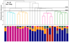 |
Fig. 15 Same as Fig. 8 but for the solar vicinity sample, considering only the accreted particles for Au. 27. |
4.4.2 Properties of the groups of clusters
What about grouping clusters together? Fig. 15 exemplifies the results for Au. 27. While in this case the majority of clumps have a clear dominant progenitor, and some clusters are well grouped together in the first passes of the single-linkage through the Mahalanobis distance, it is difficult to find a common threshold that gives the desired result for each group. For example, a threshold of DM,th = 4 would group together all the clusters where Prog. 3 is dominant and the majority of those containing Prog. 1; at the same time, clusters related to Prog. 4 would be ingested in the group where Prog. 1 is dominant in most clusters. A lower threshold of DM,th = 3.5 would instead produce an overestimated number of groups by forming two separate groups dominated by Prog. 3, and an even lower threshold of DM,th = 3 would not link the majority of the clusters dominated by Progs. 1 and 4 to any group. While each simulated galaxy has its own specificity, these general trends are common across the halos analysed. For comparison with the observations, we find that excluding in situ particles and using the D23 threshold, the completeness is ~0.25 in all the simulations, compared to ~0.6 in Au. 24 and Au. 27 when in situ particles are included. On the other-hand, the purity does not change significantly, regardless of the definition used, except for Au. 24 where the purity of the groups goes up to 𝒫g = 0.64 (compared to 0.45 previously). To reach a completeness of 0.57 in Au. 27, i.e. similar to the value found with the inclusion of in situ particles in Sect. 4.3 using the threshold of D23, the Mahalanobis distance threshold have to be increased to 3.9. In that case, the average cluster purity within groups is of 𝒫cg = 0.96 and the average purity of the groups is of 𝒫g = 0.50, slightly lower than when the in situ stars are included.
As mentioned earlier, RL22 used the MDF and the colour distribution of clusters to help increase purity and completeness of their progenitors. Several other studies have also used, either partially or exclusively, chemical properties to identify groups of stars (e.g. Horta et al. 2021, 2024; Naidu et al. 2020, 2021, Bokyoung, in prep.), or of globular clusters that originate from the same accreted galaxy (e.g. Kruijssen et al. 2019; Massari et al. 2019, 2023). Since we are working with stellar particles, we have access to the stellar age of individual particles, and we therefore decided to use the ADF instead of the colour. Following the procedure of RL22, we compare the MDF and the ADF of each cluster with the others using a Kolmogorov-Smirnov (KS) statistical test. We assume that the distributions between two clusters are compatible when the KS p-value P(ϕ1, ϕ2) > 0.05 for both the MDF and the ADF.
As shown in Fig. 16, the comparison between the MDF of the clusters reveals that approximately 60%10 of the cluster pairs with p-values >0.05 are true positives (i.e. clusters dominated by the same progenitor; green cells). In the case of Au. 23, this rate increases to 95% due to most clusters being dominated by Prog. 1. For the other halos, about 75% of the negative MDF comparisons are true negatives (i.e. pairs of clusters not dominated by the same progenitor and with p-values <0.05; white cells). In about 25% of cases, this method yields false negatives (i.e. exclusion of clusters with the same progenitor; grey cells), and in roughly 40% of cases, it produces false positives (i.e. associating clusters not dominated by the same progenitor but with similar MDFs; red cells). Interestingly, we systematically detect false positives within groups across all simulations (highlighted by the orange rectangles). In some cases, two clusters with a similar MDF show a significant contribution from the dominant progenitor of the other cluster in the pair (e.g. Cls. 59, 60, and 74 of Au. 23). However, in other cases, clusters grouped together with a similar MDF are not populated at all by stars from the same progenitors (e.g. in Au. 27 with Cl. 17, which is dominated by Prog. 4, and where Prog. 1 contributes only 5% of the cluster population, and Cls. 12 and 13, which are dominated by Prog. 1 and contain no particles from Prog. 4). Furthermore, this phenomenon cannot be solely attributed to small number statistics, as false negatives occur also in clusters populated by several hundred particles (e.g. Cls. 4 and 18 of Au. 27, although in that case, the clusters are not dynamically grouped).
The comparison of the ADF presented in Fig. 17 shows a similar ratio of true positives, generally around ~60%, except for Au. 23. However, the ADF comparison appears to be less prone to false negatives (grey cells), with a true negative ratio of approximately 90%. When comparing the ADF of individual clusters, a mix of true negatives and false positives emerges, regardless if the clusters are associated or not into dynamical groups. Across all simulations, this behaviour seems to complement the MDF results, though this is not systematic (e.g. Cl. 23 in Au. 24). Thus, by using both the MDF and ADF, it may be possible to identify intruder clusters that are not dominated by the same progenitor as the other clusters in the group, as well as to find groups of clusters potentially populated by the same progenitor. This suggests that a promising approach could be to directly compare the age-metallicity relation, as was recently done by Dodd et al. (2024) with Sequoia and Thamnos.
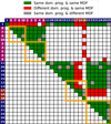 |
Fig. 16 Confusion matrix of the KS test, comparing the MDF of each significant cluster found in Au. 27 considering only particles from accreted progenitors. The green cells indicate pairs of clusters sharing the same dominant progenitor and which have a similar MDF at the 95% confidence level (p-value >0.05, true positive). The red cells show pairs of clusters with a similar MDF but with different dominant progenitor (false positive). The grey cells show the pair of clusters with the same dominant progenitor but with different MDF at the 95% confidence level (false negative). The pair of clusters that are not dominated by the same progenitor and that have not the same MDF at the 95% confidence level (true negative) are shown by the white cells. As the matrix is diagonally symmetric, we decided to not colour code the cells in the lower part of the matrix for visibility reasons. The orange rectangles show the groups of clusters linked together by the Mahalanobis distance using the same cut-off value of D23. The clusters are ordered in the same way that in Fig. 8, with their reference ID. indicated in each row and column. |
5 The impact of the artificial background halos
Several hints in the previous sections suggest that the cluster detection method might generate artificial significant clusters that do not accurately reflect the actual structure of the local stellar halo. First, unlike the debris of accreted galaxies, in situ particles are not expected to be particularly clustered in the IoM. It is true that resonances caused by non-axisymmetric features such as the bar or spiral arms can form overdensities in the IoM (Dillamore et al. 2024). However, these overdensities are expected to be relatively large, not well clustered (particularly in L⊥) and mostly found in the prograde region. Despite this, we detected significant clusters mostly populated by in situ particles in all the simulations (see Sect. 4.1), not only in those where the main galaxy is barred (see Table 2 of Grand et al. 2024). Furthermore, we detected clusters dominated by in situ stars not only in the prograde regions but also on non-rotating and on retrograde orbits (see Sect. 4.2).
Secondly, we do not observe a strong correlation between the significance and purity of the clusters, as we might naturally expect if the significant clusters were primarily composed of particles from a single accretion event. Additionally, this lack of correlation cannot be only attributed to the presence of misclassified in situ particles born in accreted gas clouds since even when in situ particles are excluded, this correlation between the purity and significance of the clusters is not observed.
Finally, if a significant cluster is predominantly populated by particles from a single accretion event, we would expect that the purity should increase if the selection is restricted to the inner part of the cluster, as the contamination should gradually dominate (in terms of relative fraction) further away from the centre of the cluster. However, we did not observe a significant change in the purity of the clusters when restricting the selection to a maximum Mahalanobis distance of 2.13 from the cluster centre, compared to the original and less restrictive selection (last paragraph of Sect. 4.1).
Here, we explore whether some of the detected clusters might be artificially originated by the method used to create the background halos. As discussed in Sect. 3.3, these background halos are generated by reshuffling the velocities of the real halo. However, this method does not adequately preserve the large-scale structure of the IoM space, and can instead lead to the creation of local over/underdensities in the IoM space of the artificial halos compared to the original ones. This issue is clearly visible in the toy model presented in Fig. 18. The original halo in this simple model consists of 1000 particles, equally spaced along the 3D Cartesian X-axis between a radius of 5.5 and 10.5 kpc (i.e. ±2.5 kpc from the Sun located at R⊙ = 8 kpc). These particles are on perfectly circular orbits within an axisymmetric Galactic potential well described by the McMillan (2017) potential. Additionally, 100 particles, all located at X = 8 kpc and equally spaced in energy, are modelled with velocity only along the vertical axis11. As shown in this figure, the distribution in energy-angular momentum of the artificial halo is locally very different compared to the original distribution. The velocity reshuffling process creates noticeable discrepancies in the IoM distribution compared to the original distribution. In the artificial halo, we clearly observe the appearance of underpopulated regions, particularly in the non-rotating, high-energy areas, and overpopulated regions, especially in the prograde high-energy region. While the specific location of these over- and underdensities depends on the specific IoM distribution of the original halo, this extremely simplistic model clearly highlights the limitations of the reshuffling method in creating artificial halos and suggests that it may contribute to the detection of artificial clusters that do not accurately reflect the true structure of the local stellar halo.
To investigate further where we can expect this artificial structures to be located, we decided to use a more realistic, yet smooth model of the MW, using the Besançon Galactic model (BGM; Robin et al. 2012; Fernández-Trincado 2017). We selected stellar particles from the solar vicinity using the same criteria as L22 and D23 to select the kinematic stellar halo and to generate the set of 100 artificial background. We computed the local significance of the original halo in each pair of IoM parameters by comparing the number of stars in the original halo to a set of 100 artificial halos, as explained in Sect. 3. The creation of the over- and under-dense regions in the artificial halos corresponds to the regions with negative and positive significance in Fig. 19, respectively. When compared to Au. 27, we see a clear similarity in the location of regions of high and low significance between the two models. In particular, in the prograde region (Lz > 0), we observe that at high vertical angular momentum, the significance is very high, indicating underpopulated artificial halos, and a region of lower angular momentum where the significance is negative, indicating overpopulated artificial halos. Interestingly, in the retrograde halo (Lz < 0), we observe the inverse trend, with a region of positive significance at low energy and low vertical angular momentum, although the absolute amplitude of the significance is lower, likely due to the smaller number of particles in this region. We can observe some similarities between the regions of high significance in these two models and the locations of some significant clusters detected by L22 and D23 in the MW, and conversely, between the low-significance regions and the absence of significant clusters. These analyses raise the question of the reality of some detected structures in the observations.
It would be interesting to explore alternative methods for generating artificial backgrounds that avoid the biases of the current approach. Some potential directions include modelling the background halo based on an assumed potential and distribution function that reproduces the MW’s global properties well (e.g. BGM or a self-consistent model based on McMillan 2017), or using a multi-Gaussian model to describe the IoM space of the background. However, developing and testing such methods is beyond the scope of this paper, which focuses on quantifying the performance of the current technique. Nevertheless, the work presented here provides a useful metric for evaluating the performance of these alternative approaches.
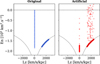 |
Fig. 18 Toy model illustrating the over- and under-dense regions in the IoM of an artificial halo (right panel) created by reshuffling the velocities of the original particles (left panel). In the original distribution, 1000 particles are on perfectly circular orbits and 100 particles on perfectly vertical orbits. In both panels, black lines delineate the possible distribution limits in energy-angular momentum, and the dashed line indicates the energy limit for a particle to be considered bound. |
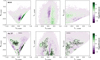 |
Fig. 19 Variation in the significance in the IoM of the originally kinematically selected halo in the solar vicinity of the BGM (upper panels) and of Au. 27 (lower panels) compared to the set of 100 artificial halos. In the lower row, the ellipses indicate the location of the significant clusters detected by the single linkage method using the in situ and accreted particles. |
6 Discussion and conclusions
In this paper, we analyse the performance of one of the most advanced methods for identifying the debris of past accreted galaxies in the local stellar halo by applying it to four Milky Way-like galaxies from the Auriga simulation suite. This method, described in detail in L22, is aimed at identifying significant clumps of stars in the IoM space by comparing the local number of stars within a predetermined region with a suite of N artificial background halos.
Although this method is very promising and has proven its capability to identify both known and new structures (Lövdal et al. 2022; Ruiz-Lara et al. 2022; Dodd et al. 2023), we demonstrate here (see Sect. 5) that the method used to generate the artificial background halos can produce local density variations that are not representative of the smooth background distribution in the original halo. This can ultimately lead to an artificial boost in the significance for some clusters, or even to the detection of artificial significant clusters (particularly in highly prograde or retrograde-low energy regions), while potentially preventing the detection of significant clusters in other regions.
Setting aside this potential source of error, we found that the method of detecting significant clusters is also limited and does not allow for the recovery of most of the debris left by accreted galaxies. Indeed, in Sect. 4.1, we observed that this method is particularly effective in identifying most of the stellar particles originating from a progenitor that was recently accreted (within the last 6–7 Gyr). However, it fails at recovering most of the debris left by the older accretions, regardless of the actual mass of the progenitor. In fact, most of the particles from these older accretions detected as being part of any cluster tend to actually contaminate the debris left by other accreted galaxies or by particles formed in situ. Even when the detection of the clusters was performed only with accreted particles, the method still largely identifies the debris left by the most recent accretions; however, debris left over by older accretions remain mostly undetected (see Sect. 4.4). The only exception is that in this case, it also identifies some particles originating from the accreted galaxy that contributes the most to the local stellar halo. Nevertheless, other accreted galaxies mostly end up undetected. This suggests that in a cosmologically motivated context, debris from the oldest accretion does not remain strongly clumped in the IoM in the solar vicinity. As mentioned in Sect. 3, the debris left by accreted galaxies with stellar mass of ~106 M⊙ might not be detected by the algorithm due to the imposed minimum number of cluster members and the simulation resolution. However, the observed bias favouring the detection of more recent accretion events should still apply to these smaller progenitors, since low-mass accreted galaxies passing through the solar vicinity are more susceptible to disruption than their more massive counter-parts. A similar trend was reported by Wu et al. (2022), who found that the Enlink algorithm applied to MW-like galaxies in the FIRE-2 simulations also preferentially detected debris from more recent accretion events.
We also found that the vast majority of the significant clusters in the IoM space identified by this method are highly contaminated by in situ particles, when the fact is that the latter are not the most important population. Additionally, almost all the clusters are populated by stars from more than one accreted galaxy, with clusters where 90% of the stars originate from the same progenitor being very rare. Even with the inclusion of chemical and stellar age information (see Sect. 4.2), we found it challenging to disentangle clusters dominated by in situ particles from those dominated by accreted particles. The distinction is clearer for prograde clusters, where in situ clusters are more metalrich, younger, and more [Mg/Fe] depleted than their accreted counterparts. However, for clusters with Lz < 500 km s−1 kpc−1, the distinction becomes less clear, as both in situ and accreted particle-dominated clusters exhibit similar behaviour in metallicity, [Mg/Fe], and stellar age. We tentatively suggest that all clusters with a median metallicity lower than [Fe/H] < −1.35 are dominated by accreted particles. Nevertheless, in the few clusters identified below that limit, we found that the contamination from in situ particles is still as high as 30%, although this conclusion is drawn from a very limited sample of clusters. Furthermore, most of the clusters dominated by accreted particles have a metallicity higher than this, although this can also be partially explained by the fact that smaller accreted galaxies are not well resolved by the Auriga simulations. Thus, we can expect that in reality, the ratio of cluster with [Fe/H] < −1.35 might be more important.
It is possible to group together clusters closed to each other in the IoM space, as done by RL22 and D23, in observations. However, as presented in Sect. 4.3, the purity of these groups decreases rapidly, by linking together clusters dominated by different progenitors. The simulations suggest about a third of the groups found by D23 might consist of clusters dominated by different accreted galaxies. Furthermore, even in such a small region as in the solar vicinity, the debris of a single old accreted galaxy are spread over a wide region of the IoM space. As a result, several distinct groups can be mostly populated by particles originating from a single accreted galaxy. Our results suggest that up to 40% of the clusters not grouped together using the threshold of D23 to identify groups might actually be coming from the same accreted galaxy, although we see a great variation in this value from galaxy to galaxy.
RL22 proposed that clusters from the same galaxy can be identified and distinguished from those originating from different galaxies by comparing their metallicity distributions. In Sect. 4.4, we show that metallicity alone is insufficient for this purpose, as clusters dominated by different galaxies can have similar distribution of metallicity, while clusters dominated by the same galaxy can have different distribution of metallicities, even within the same dynamical group. This last point aligns with expectations of metallicity gradients with energy in accreted galaxies (Amarante et al. 2022; Horta et al. 2023; Mori et al. 2024). Our analysis clearly shows that such a gradient is to be expected, even in such a small volume around the Sun. A similar pattern is observed when comparing age distributions. However, our results suggest that combining age and metallicity distributions may effectively disentangle clusters dominated by similar or different progenitors. This is particularly promising given the recent availability to derive precise age-metallicity relations for populations located within the solar neighbourhood (e.g. Gallart et al. 2024, Fernandez-Alvar, in prep.), even for a limited sample of stars (Dodd et al. 2024).
Applying these conclusions to structures identified in the local stellar halo of the MW allows us to hypothesise about their independence, reality, and progenitor characteristics, and to revisit the MW accretion history. A first hypothesis can be made concerning the group formed by Sequoia (Myeong et al. 2019) and L-RL64/Antaeus (Lövdal et al. 2022; Ruiz-Lara et al. 2022; Oria et al. 2022), which were grouped together using the distance threshold of L22 but identified as separate structures using the more restrictive threshold of D23. We found that with the threshold used by D23, the purity of groups increases by a factor three compared to when the threshold of L22 is used, while the group completeness does not change significantly. As such, our results go in the direction of the conclusion drawn by RL22 that these structures are not related to each other. Moreover, since both Sequoia and L-RL64/Antaeus are retrograde, with average metallicities of [Fe/H] = −1.47 and [Fe/H] = −1.67, respectively (Bellazzini et al. 2023; Dodd et al. 2023), we can confirm that these structures are dominated by accreted particles.
Regarding Sequoia, RL22 found it to be composed by two clusters, the most significant of which has a significance of 9.29, justified by the clear overdensity it formed in the E-Lz space. In our simulations, all clusters dominated by accreted particles with such a high significance are systematically formed by galaxies accreted less than 6 Gyr ago. Therefore, we suggest that the progenitor of Sequoia might have been accreted within the last 6 Gyr, which is more recent than the usually assumed time frame (≈9 Gyr ago, Myeong et al. 2019). This contrasts with the accretion time of the progenitor galaxy at z ~ 2 that led to the Sequoialike feature in the E-Lz space found by García-Bethencourt et al. (2023) in their simulations. It has been suggested that Sequoia, along with other structures such as Arjuna, L’Itoi, and LMS-1, might be related to GES based on their chemistry (Koppelman et al. 2020; Naidu et al. 2020, 2021). However, it is largely accepted that the progenitor of GES has been accreted 8–11 Gyr ago (Helmi et al. 2018; Di Matteo et al. 2019; Gallart et al. 2019, but see Donlon et al. 2024), at least 2 Gyr earlier than our estimation for the progenitor of Sequoia. Therefore, it is very unlikely that GES and Sequoia are the signatures of the same accreted galaxy, or that the Sequoia progenitor was a satellite of GES as proposed by Naidu et al. (2021). Furthermore, our results clearly show that it can be hazardous to claim that structures are related together only based on the distribution of metallicity; particular in the case of GES and Sequoia, since Matsuno et al. (2022) found that they both have different chemical trends using high-resolution spectroscopic measurement.
Regarding the Helmi stream (Helmi & White 1999), it is a prograde structure with a median metallicity of [Fe/H] = −1.52 (Bellazzini et al. 2023). Following our results, we can unsurprisingly confirm its accreted nature. Furthermore, in L22, it is identified by two significant clusters, with the highest one having a significance of S = 9.83. It is likely that this value is underestimated, as the Helmi stream is located in a region of the IoM space where the artificial halos tend to be overpopulated (see Sect. 5). In all the cases, as for Sequoia, such a high significance suggests that its progenitor galaxy was accreted within the last 6 Gyr. This accretion time is on the lower edge of the estimation obtained in previous works (Kepley et al. 2007; Koppelman et al. 2019b, 5–9 Gyr).
Another structure identified by both L22 and D23 is Thamnos. It was first identified by Koppelman et al. (2019b) as two distinct structures, Thamnos 1 and 2, in the IoM space. However, based on their dynamical and chemical properties, it has been suggested that these two structures likely originate from the same accreted galaxy, with a stellar mass of approximately 5 × 10⁶ M⊙ (Koppelman et al. 2019b; Ruiz-Lara et al. 2022). Both L22 and D23 identify Thamnos as a group of several clusters linked under the same dynamical group. Bellazzini et al. (2023) measured a median metallicity of [Fe/H] = −1.22 for the stars belonging to the Thamnos group identified by L22, which is slightly higher than the values reported by RL22 for Thamnos 1 and 2, of [Fe/H] = −1.42 and −1.30, respectively. This relatively high metallicity in the retrograde region suggests that Thamnos may not necessarily be dominated by accreted particles, but rather could have a substantial contribution from in situ particles. Even if Thamnos is mainly composed of accreted stars, the contamination from in situ particles could be significant, potentially around 40%, as indicated by Fig. 10. This high level of contamination by in situ particles is in agreement with the recent estimation of Dodd et al. (2024). Furthermore, in L22, the three clusters that they are located in a region of the IoM space where the significance can be overestimated due to the under-population of the artificial halos in that region, although this is not the case in all the simulations. In the four simulations studied here, all the clusters found in that region of the IoM space have a similar significance between 3 and 3.5, and are populated between 30% and up to 80% of in situ particles. Furthermore, even by putting aside the contribution of in situ particles, most of these clusters are populated by particles from two progenitors, with a population ratio of ~30%. The only exception is in Au.23, where 75–80% of the particles are from a single progenitor. Therefore, we caution against the assumption that Thamnos is a clear significant structure left by a single accreted galaxy. Instead, it may be a composite structure formed by several accreted galaxies and in situ stars, which could explain its unique chemical properties that differ from any other substructures found in the stellar halo (Horta et al. 2023). At the current stage, we are not able to favour one possibility over the other, although it seems clear that the region of Thamnos is highly contaminated by in situ particles. Further research, particularly focusing on the promising age-metallicity relation developed by Dodd et al. (2024), and leveraging future data from Gaia, as well as upcoming large spectroscopic surveys such as DESI-MWS (Cooper et al. 2023), WEAVE (Jin et al. 2024), and 4-MOST (de Jong et al. 2010), will be essential to clarify the reality of the Thamnos structure.
Another point is regarding the L-RL3 structure (Cl. 3 of L22). It is a prograde cluster located at low energy with a median metallicity of [Fe/H]=−0.70 (Bellazzini et al. 2023), composed of 2137 stars and a significance of 6.3. In all the simulations when in situ particles are considered, the clusters with more than 1000 particles are highly populated by in situ particles (>40%), and are usually dominated by them. Given this fact and considering its high median metallicity, we favour the hypothesis made by RL22 that they are mostly populated by in situ particles. Even by selection of the particles of the clusters with [Fe/H] < −1.0, we found that ≃30% of the particles are flagged as in situ and that the accreted particles originate from two different progenitors with a contribution ratio to accreted particles of typically 60% and 30%, respectively. As such, we suggest that L-RL3 is not a structure formed by a single accreted galaxy and that it has been formed, instead, by the accumulation of in situ and accreted particles. It is possible that L-RL3 is an artificial cluster created by the under-population of the artificial background halos at its location.
Finally, our simulations tentatively suggest that well-defined structures in the E-Lz space within the solar vicinity, which are identifiable by eye, such as ED-2 (Dodd et al. 2023; Balbinot et al. 2023), ED-4/Typhoon (Tenachi et al. 2022), and possibly Shakti (Malhan & Rix 2024), may have been created by galaxies accreted relatively recently (within the last 6–7 Gyr). We find no evidence of similarly well-defined structures originating from older, even very massive, galaxies (see Fig. 4). However, these structures are assumed to be the debris left by accreted galaxies several order of magnitude less massive than the ones studied here. Therefore, it is possible that the current state-of-the art cosmological simulations such as Auriga are not able to resolve the dynamical imprint left by such small galaxies over several gigayears, although they are able to resolve dwarf galaxies and stellar streams down to 106 M⊙ (see Grand et al. 2024; Riley et al. 2025, but also Panithanpaisal et al. 2021; Cunningham et al. 2022; Shipp 2023; Horta et al. 2024 for other cosmological suite of similar resolution). Furthermore, in these simulations, there remains uncertainty related to several aspects of the physics models, such as chemical enrichment, yields, and feedback processes, which could influence the detailed chemical patterns of the stellar debris. It will be interesting in the near future to study the survivability of these structures in the current simulations.
Another potential caveat of our analysis concerns the possible presence of misclassified in situ stars that may actually have originated from accreted gas clouds. This misclassification could have several significant implications for the conclusions drawn from our study, depending on the actual ratio of misclassified in situ stars. For instance, it might explain the high contamination by in situ particles observed in Sect. 4.1. Similarly, it could account for the predominance of in situ particles in the majority of significant clusters, regardless of their orbital properties. This misclassification might also shed light on why clusters dominated by in situ and accreted particles exhibit similar chemical properties and stellar formation ages, particularly in the case of retrograde clusters. However, in this context, if the fraction of misclassified in situ particles is substantial, we would expect to observe differences in the distribution of stellar ages between misclassified in situ particles and correctly identified accreted particles. Indeed, for a given accretion event, the accreted stars are expected to form before the gas is stripped from the accreted galaxy, while the misclassified in situ stars would be born shortly afterward. Yet, in the identified significant clusters, we did not find that in situ stars were systematically younger than the accreted ones. Identifying which in situ particles might be misclassified is a challenging task within the AURIGA simulations due to the mesh-based hydrodynamical approach employed by AREPO (Weinberger et al. 2020), the code used to run these simulations. This approach does not directly allow the origin of gas to be tracked. We plan to revisit the accreted versus in situ classification in the Auriga simulations in a future work dedicated to this task.
In conclusion, the accretion history of the MW is still far from well established, with several structures identified in the stellar halo near the solar vicinity having potentially been misinterpreted as accreted or not originating from a single accretion event. Our results question the reality of several detected structures assumed to be formed by the disruption of an accreted galaxy. Multiple scenarios could explain the observed dynamical, chemical, and stellar age properties of these structures. The upcoming Gaia data release, along with medium and high-resolution spectroscopic observations from DESI-MWS (Cooper et al. 2023), WEAVE (Jin et al. 2024), and 4-MOST (de Jong et al. 2010), will significantly enhance our understanding of the accretion history of the MW by allowing us to probe more distant regions, which have been less affected by in situ stars and where the dynamical timescale (and, thus, the surviving time of the dynamical debris left by accreted galaxies) is longer (Binney & Tremaine 2008). However, as this study demonstrates, it is crucial to compare these datasets and the methods used to analyse them with cosmologically motivated simulations. Such comparisons are essential for evaluating the effectiveness of the methods developed to identify these structures and for determining their origins within the broader context of galactic evolution.
Data availability
Figures 8, 4, 16, and 17, together with the supplementary figures showing the identified significant clusters, their parameters, and the mock catalogues created for each analysed simulation, are available here: https://zenodo.org/records/17276763.
Acknowledgements
The authors want to thank C. Chiappini, T. Callingham, E. Dodd, A. Helmi, V. Hill, S. Lövdal, and D. Massari, for useful discussions, and comments, and their strong support. They also thank the anonymous referee for her/his careful reading of the paper and for her/his interesting comments and suggestions that helped improving its quality. GFT and GB acknowledge support from the Agencia Estatal de Investigación del Ministerio de Ciencia en Innovación (AEI-MICIN) and the European Regional Development Fund (ERDF) under grant number PID2020-118778GB-I00/10.13039/501100011033 and the AEI under grant number CEX2019-000920-S. RG acknowledges financial support from an STFC Ernest Rutherford Fellowship (ST/W003643/1). This work uses simulations from the Auriga Project public data release (Grand et al. 2024) available at https://wwwmpa.mpa-garching.mpg.de/auriga/gaiamock.html.
References
- Abdurro’uf, Accetta, K., Aerts, C., et al. 2022, ApJS, 259, 35 [NASA ADS] [CrossRef] [Google Scholar]
- Amarante, J. A. S., Beraldo e Silva, L., Debattista, V. P., & Smith, M. C. 2020, ApJ, 891, L30 [NASA ADS] [CrossRef] [Google Scholar]
- Amarante, J. A. S., Debattista, V. P., Beraldo e Silva, L., Laporte, C. F. P., & Deg, N. 2022, ApJ, 937, 12 [NASA ADS] [CrossRef] [Google Scholar]
- Amorisco, N. C. 2017, MNRAS, 469, L48 [Google Scholar]
- Balbinot, E., Helmi, A., Callingham, T., et al. 2023, A&A, 678, A115 [NASA ADS] [CrossRef] [EDP Sciences] [Google Scholar]
- Bellazzini, M., Massari, D., De Angeli, F., et al. 2023, A&A, 674, A194 [NASA ADS] [CrossRef] [EDP Sciences] [Google Scholar]
- Belokurov, V., & Kravtsov, A. 2022, MNRAS, 514, 689 [NASA ADS] [CrossRef] [Google Scholar]
- Belokurov, V., Deason, A. J., Koposov, S. E., et al. 2018, MNRAS, 477, 1472 [Google Scholar]
- Belokurov, V., Sanders, J. L., Fattahi, A., et al. 2020, MNRAS, 494, 3880 [Google Scholar]
- Binney, J., & Tremaine, S. 2008, Galactic Dynamics, 2nd edn. [Google Scholar]
- Bland-Hawthorn, J., & Gerhard, O. 2016, ARA&A, 54, 529 [Google Scholar]
- Blumenthal, G. R., Faber, S. M., Primack, J. R., & Rees, M. J. 1984, Nature, 311, 517 [Google Scholar]
- Bonaca, A., Conroy, C., Wetzel, A., Hopkins, P. F., & Kereš, D. 2017, ApJ, 845, 101 [NASA ADS] [CrossRef] [Google Scholar]
- Borsato, N. W., Martell, S. L., & Simpson, J. D. 2020, MNRAS, 492, 1370 [NASA ADS] [CrossRef] [Google Scholar]
- Bovy, J., Rix, H.-W., Liu, C., et al. 2012, ApJ, 753, 148 [Google Scholar]
- Brown, A. G. A., Velázquez, H. M., & Aguilar, L. A. 2005, MNRAS, 359, 1287 [NASA ADS] [CrossRef] [Google Scholar]
- Buder, S., Sharma, S., Kos, J., et al. 2021, MNRAS, 506, 150 [NASA ADS] [CrossRef] [Google Scholar]
- Buist, H. J. T., & Helmi, A. 2015, A&A, 584, A120 [NASA ADS] [CrossRef] [EDP Sciences] [Google Scholar]
- Carollo, D., Beers, T. C., Lee, Y. S., et al. 2007, Nature, 450, 1020 [NASA ADS] [CrossRef] [Google Scholar]
- Carollo, D., Beers, T. C., Chiba, M., et al. 2010, ApJ, 712, 692 [NASA ADS] [CrossRef] [Google Scholar]
- Carrillo, A., Deason, A. J., Fattahi, A., Callingham, T. M., & Grand, R. J. J. 2024, MNRAS, 527, 2165 [Google Scholar]
- Ceccarelli, E., Massari, D., Mucciarelli, A., et al. 2024, A&A, 684, A37 [NASA ADS] [CrossRef] [EDP Sciences] [Google Scholar]
- Chabrier, G. 2003, PASP, 115, 763 [Google Scholar]
- Chandra, V., Semenov, V. A., Rix, H.-W., et al. 2023, The Three-Phase Evolution of the Milky Way [Google Scholar]
- Conselice, C. J. 2014, ARA&A, 52, 291 [CrossRef] [Google Scholar]
- Cooper, A. P., Koposov, S. E., Prieto, C. A., et al. 2023, ApJ, 947, 37 [NASA ADS] [CrossRef] [Google Scholar]
- Costantin, L., Pérez-González, P. G., Guo, Y., et al. 2023, Nature, 623, 499 [NASA ADS] [CrossRef] [Google Scholar]
- Cunningham, E. C., Sanderson, R. E., Johnston, K. V., et al. 2022, ApJ, 934, 172 [NASA ADS] [CrossRef] [Google Scholar]
- Dalton, G., Trager, S. C., Abrams, D. C., et al. 2012, SPIE Conf. Ser., 8446, 84460P [Google Scholar]
- Das, P., Hawkins, K., & Jofré, P. 2020, MNRAS, 493, 5195 [NASA ADS] [CrossRef] [Google Scholar]
- Davison, T. A., Norris, M. A., Leaman, R., et al. 2021, MNRAS, 507, 3089 [NASA ADS] [CrossRef] [Google Scholar]
- de Jong, J. T. A., Yanny, B., Rix, H.-W., et al. 2010, ApJ, 714, 663 [NASA ADS] [CrossRef] [Google Scholar]
- de Jong, R. S., Agertz, O., Berbel, A. A., et al. 2019, The Messenger, 175, 3 [NASA ADS] [Google Scholar]
- Deason, A. J., & Belokurov, V. 2024, Galactic Archaeology with Gaia [Google Scholar]
- Debattista, V. P., Roškar, R., Valluri, M., et al. 2013, MNRAS, 434, 2971 [NASA ADS] [CrossRef] [Google Scholar]
- Di Matteo, P., Haywood, M., Lehnert, M. D., et al. 2019, A&A, 632, A4 [NASA ADS] [CrossRef] [EDP Sciences] [Google Scholar]
- Dillamore, A. M., Belokurov, V., & Evans, N. W. 2024, MNRAS, 532, 4389 [NASA ADS] [CrossRef] [Google Scholar]
- Dodd, E., Callingham, T. M., Helmi, A., et al. 2023, A&A, 670, L2 [NASA ADS] [CrossRef] [EDP Sciences] [Google Scholar]
- Dodd, E., Ruiz-Lara, T., Helmi, A., et al. 2024, Characterisation of Local Halo Building Blocks: Thamnos and Sequoia [Google Scholar]
- Donlon, T., Newberg, H. J., Sanderson, R., et al. 2024, MNRAS, 531, 1422 [NASA ADS] [CrossRef] [Google Scholar]
- D’Souza, R., & Bell, E. 2018, MNRAS, 474, 5300 [CrossRef] [Google Scholar]
- Duan, Q., Conselice, C. J., Li, Q., et al. 2024, arXiv e-prints [arXiv:2407.09472] [Google Scholar]
- Eggen, O. J., Lynden-Bell, D., & Sandage, A. R. 1962, ApJ, 136, 748 [NASA ADS] [CrossRef] [Google Scholar]
- Eilers, A.-C., Hogg, D. W., Rix, H.-W., & Ness, M. K. 2019, ApJ, 871, 120 [Google Scholar]
- Everitt, B., Landau, S., Leese, M., & Stahl, D. 2011, Cluster Analysis, 5th Edition (John Wiley & Sons) [Google Scholar]
- Fattahi, A., Belokurov, V., Deason, A. J., et al. 2019, MNRAS, 484, 4471 [NASA ADS] [CrossRef] [Google Scholar]
- Faucher-Giguère, C.-A., Lidz, A., Zaldarriaga, M., & Hernquist, L. 2009, ApJ, 703, 1416 [Google Scholar]
- Fernandes, L., Mason, A. C., Horta, D., et al. 2023, MNRAS, 519, 3611 [NASA ADS] [CrossRef] [Google Scholar]
- Fernández-Trincado, J. G. 2017, PhD thesis, Université de Franche-Comté, France [Google Scholar]
- Feuillet, D. K., Feltzing, S., Sahlholdt, C. L., & Casagrande, L. 2020, MNRAS, 497, 109 [Google Scholar]
- Font, A. S., Johnston, K. V., Bullock, J. S., & Robertson, B. E. 2006, ApJ, 646, 886 [NASA ADS] [CrossRef] [Google Scholar]
- Freeman, K., & Bland-Hawthorn, J. 2002, ARA&A, 40, 487 [Google Scholar]
- Gaia Collaboration (Brown, A. G. A., et al.) 2018, A&A, 616, A1 [NASA ADS] [CrossRef] [EDP Sciences] [Google Scholar]
- Gallart, C., Bernard, E. J., Brook, C. B., et al. 2019, Nat. Astron., 3, 932 [NASA ADS] [CrossRef] [Google Scholar]
- Gallart, C., Surot, F., Cassisi, S., et al. 2024, A&A, 687, A168 [NASA ADS] [CrossRef] [EDP Sciences] [Google Scholar]
- Garavito-Camargo, N., Besla, G., Laporte, C. F. P., et al. 2021, ApJ, 919, 109 [NASA ADS] [CrossRef] [Google Scholar]
- García-Bethencourt, G., Brook, C. B., Grand, R. J. J., & Kawata, D. 2023, MNRAS, 526, 1190 [CrossRef] [Google Scholar]
- Gilbert, K. M., Kalirai, J. S., Guhathakurta, P., et al. 2014, ApJ, 796, 76 [NASA ADS] [CrossRef] [Google Scholar]
- Gilmore, G., Randich, S., Worley, C. C., et al. 2022, A&A, 666, A120 [NASA ADS] [CrossRef] [EDP Sciences] [Google Scholar]
- Gómez, F. A., & Helmi, A. 2010, MNRAS, 401, 2285 [Google Scholar]
- Gómez, F. A., Helmi, A., Brown, A. G. A., & Li, Y.-S. 2010, MNRAS, 408, 935 [Google Scholar]
- Gómez, F. A., Minchev, I., O’Shea, B. W., et al. 2012, MNRAS, 423, 3727 [CrossRef] [Google Scholar]
- Gómez, F. A., Minchev, I., O’Shea, B. W., et al. 2013, MNRAS, 429, 159 [Google Scholar]
- Gómez, F. A., White, S. D. M., Marinacci, F., et al. 2016, MNRAS, 456, 2779 [Google Scholar]
- Gómez, F. A., Grand, R. J. J., Monachesi, A., et al. 2017, MNRAS, 472, 3722 [CrossRef] [Google Scholar]
- Grand, R. J. J., Gómez, F. A., Marinacci, F., et al. 2017, MNRAS, 467, 179 [NASA ADS] [Google Scholar]
- Grand, R. J. J., Helly, J., Fattahi, A., et al. 2018, MNRAS, 481, 1726 [Google Scholar]
- Grand, R. J. J., Deason, A. J., White, S. D. M., et al. 2019, MNRAS, 487, L72 [Google Scholar]
- Grand, R. J. J., Fragkoudi, F., Gómez, F. A., et al. 2024, MNRAS, 532, 1814 [NASA ADS] [CrossRef] [Google Scholar]
- Gravity Collaboration (Abuter, R., et al.) 2018, A&A, 615, L15 [NASA ADS] [CrossRef] [EDP Sciences] [Google Scholar]
- Hawkins, K., Jofré, P., Masseron, T., & Gilmore, G. 2015, MNRAS, 453, 758 [NASA ADS] [CrossRef] [Google Scholar]
- Haywood, M., Di Matteo, P., Lehnert, M. D., et al. 2018, ApJ, 863, 113 [Google Scholar]
- Helmi, A. 2020, ARA&A, 58, 205 [Google Scholar]
- Helmi, A., & de Zeeuw, P. T. 2000, MNRAS, 319, 657 [Google Scholar]
- Helmi, A., & White, S. D. M. 1999, MNRAS, 307, 495 [CrossRef] [Google Scholar]
- Helmi, A., Veljanoski, J., Breddels, M. A., Tian, H., & Sales, L. V. 2017, A&A, 598, A58 [NASA ADS] [CrossRef] [EDP Sciences] [Google Scholar]
- Helmi, A., Babusiaux, C., Koppelman, H. H., et al. 2018, Nature, 563, 85 [Google Scholar]
- Horta, D., Schiavon, R. P., Mackereth, J. T., et al. 2021, MNRAS, 500, 1385 [Google Scholar]
- Horta, D., Schiavon, R. P., Mackereth, J. T., et al. 2023, MNRAS, 520, 5671 [NASA ADS] [CrossRef] [Google Scholar]
- Horta, D., Yuxi, Lu, et al. 2024, Stellar Mergers or Truly Young? IntermediateAge Stars on Highly-Radial Orbits in the Milky Way’s Stellar Halo [Google Scholar]
- Hotelling, H. 1933, J. Educ. Psychol., 24, 417 [CrossRef] [Google Scholar]
- Ibata, R. A., Gilmore, G., & Irwin, M. J. 1994, Nature, 370, 194 [Google Scholar]
- Ibata, R., Malhan, K., Tenachi, W., et al. 2024, ApJ, 967, 89 [NASA ADS] [CrossRef] [Google Scholar]
- Jean-Baptiste, I., Di Matteo, P., Haywood, M., et al. 2017, A&A, 604, A106 [NASA ADS] [CrossRef] [EDP Sciences] [Google Scholar]
- Jin, S., Trager, S. C., Dalton, G. B., et al. 2024, MNRAS, 530, 2688 [NASA ADS] [CrossRef] [Google Scholar]
- Johnston, K. V., Bullock, J. S., Sharma, S., et al. 2008, ApJ, 689, 936 [Google Scholar]
- Kepley, A. A., Morrison, H. L., Helmi, A., et al. 2007, AJ, 134, 1579 [NASA ADS] [CrossRef] [Google Scholar]
- Khoperskov, S., Minchev, I., Libeskind, N., et al. 2023a, A&A, 677, A91 [NASA ADS] [CrossRef] [EDP Sciences] [Google Scholar]
- Khoperskov, S., Minchev, I., Libeskind, N., et al. 2023b, A&A, 677, A90 [NASA ADS] [CrossRef] [EDP Sciences] [Google Scholar]
- Knebe, A., Gill, S. P. D., Kawata, D., & Gibson, B. K. 2005, MNRAS, 357, L35 [NASA ADS] [CrossRef] [Google Scholar]
- Kollmeier, J. A., Zasowski, G., Rix, H.-W., et al. 2017, SDSS-V: Pioneering Panoptic Spectroscopy [Google Scholar]
- Koppelman, H. H., & Helmi, A. 2021, A&A, 649, A55 [NASA ADS] [CrossRef] [EDP Sciences] [Google Scholar]
- Koppelman, H., Helmi, A., & Veljanoski, J. 2018, ApJ, 860, L11 [NASA ADS] [CrossRef] [Google Scholar]
- Koppelman, H. H., Helmi, A., Massari, D., Price-Whelan, A. M., & Starkenburg, T. K. 2019a, A&A, 631, L9 [NASA ADS] [CrossRef] [EDP Sciences] [Google Scholar]
- Koppelman, H. H., Helmi, A., Massari, D., Roelenga, S., & Bastian, U. 2019b, A&A, 625, A5 [NASA ADS] [CrossRef] [EDP Sciences] [Google Scholar]
- Koppelman, H. H., Bos, R. O. Y., & Helmi, A. 2020, A&A, 642, L18 [NASA ADS] [CrossRef] [EDP Sciences] [Google Scholar]
- Kordopatis, G., Recio-Blanco, A., Schultheis, M., & Hill, V. 2020, A&A, 643, A69 [NASA ADS] [CrossRef] [EDP Sciences] [Google Scholar]
- Kormendy, J., Drory, N., Bender, R., & Cornell, M. E. 2010, ApJ, 723, 54 [Google Scholar]
- Kruijssen, J. M. D., Pfeffer, J. L., Reina-Campos, M., Crain, R. A., & Bastian, N. 2019, MNRAS, 486, 3180 [Google Scholar]
- Kruijssen, J. M. D., Pfeffer, J. L., Chevance, M., et al. 2020, MNRAS, 498, 2472 [NASA ADS] [CrossRef] [Google Scholar]
- Lane, J. M. M., Bovy, J., & Mackereth, J. T. 2023, MNRAS, 526, 1209 [NASA ADS] [CrossRef] [Google Scholar]
- Laporte, C. F. P., Agnello, A., & Navarro, J. F. 2018a, arXiv e-prints [arXiv:1804.04139] [Google Scholar]
- Laporte, C. F. P., Johnston, K. V., Gómez, F. A., Garavito-Camargo, N., & Besla, G. 2018b, MNRAS, 473, 1218 [NASA ADS] [CrossRef] [Google Scholar]
- Lee, Y. S., Beers, T. C., Carlin, J. L., et al. 2015, AJ, 150, 187 [NASA ADS] [CrossRef] [Google Scholar]
- Lövdal, S. S., Ruiz-Lara, T., Koppelman, H. H., et al. 2022, A&A, 665, A57 [NASA ADS] [CrossRef] [EDP Sciences] [Google Scholar]
- Mackereth, J. T., Schiavon, R. P., Pfeffer, J., et al. 2019, MNRAS, 482, 3426 [Google Scholar]
- Mackey, D., Lewis, G. F., Brewer, B. J., et al. 2019, Nature, 574, 69 [NASA ADS] [CrossRef] [Google Scholar]
- Majewski, S. R., Skrutskie, M. F., Weinberg, M. D., & Ostheimer, J. C. 2003, ApJ, 599, 1082 [NASA ADS] [CrossRef] [Google Scholar]
- Malhan, K. 2022, ApJ, 930, L9 [NASA ADS] [CrossRef] [Google Scholar]
- Malhan, K., & Rix, H.-W. 2024, ApJ, 964, 104 [NASA ADS] [CrossRef] [Google Scholar]
- Malhan, K., Yuan, Z., Ibata, R. A., et al. 2021, ApJ, 920, 51 [NASA ADS] [CrossRef] [Google Scholar]
- Martin, N. F., Ibata, R. A., & Irwin, M. 2007, ApJ, 668, L123 [Google Scholar]
- Massari, D., Koppelman, H. H., & Helmi, A. 2019, A&A, 630, L4 [NASA ADS] [CrossRef] [EDP Sciences] [Google Scholar]
- Mateu, C. 2023, MNRAS, 520, 5225 [Google Scholar]
- Massari, D., Aguado-Agelet, F., Monelli, M., et al. 2023, A&A, 680, A20 [NASA ADS] [CrossRef] [EDP Sciences] [Google Scholar]
- Matsuno, T., Koppelman, H. H., Helmi, A., et al. 2022, A&A, 661, A103 [NASA ADS] [CrossRef] [EDP Sciences] [Google Scholar]
- McConnachie, A. W., Ibata, R., Martin, N., et al. 2018, ApJ, 868, 55 [Google Scholar]
- McMillan, P. J. 2017, MNRAS, 465, 76 [NASA ADS] [CrossRef] [Google Scholar]
- McMillan, P. J., & Binney, J. J. 2008, MNRAS, 390, 429 [NASA ADS] [CrossRef] [Google Scholar]
- Monachesi, A., Gómez, F. A., Grand, R. J. J., et al. 2019, MNRAS, 485, 2589 [NASA ADS] [CrossRef] [Google Scholar]
- Mori, A., Di Matteo, P., Salvadori, S., et al. 2024, Metallicity Distributions of Halo Stars: Do They Trace the Galactic Accretion History? [Google Scholar]
- Morrison, H. L., Helmi, A., Sun, J., et al. 2009, ApJ, 694, 130 [CrossRef] [Google Scholar]
- Myeong, G. C., Evans, N. W., Belokurov, V., Sanders, J. L., & Koposov, S. E. 2018a, MNRAS, 478, 5449 [NASA ADS] [CrossRef] [Google Scholar]
- Myeong, G. C., Evans, N. W., Belokurov, V., Sanders, J. L., & Koposov, S. E. 2018b, ApJ, 863, L28 [NASA ADS] [CrossRef] [Google Scholar]
- Myeong, G. C., Vasiliev, E., Iorio, G., Evans, N. W., & Belokurov, V. 2019, MNRAS, 488, 1235 [Google Scholar]
- Myeong, G. C., Belokurov, V., Aguado, D. S., et al. 2022, ApJ, 938, 21 [NASA ADS] [CrossRef] [Google Scholar]
- Naidu, R. P., Conroy, C., Bonaca, A., et al. 2020, ApJ, 901, 48 [Google Scholar]
- Naidu, R. P., Conroy, C., Bonaca, A., et al. 2022, Live Fast, Die α-Enhanced: The Mass-Metallicity-α Relation of the Milky Way’s Disrupted Dwarf Galaxies [Google Scholar]
- Necib, L., Ostdiek, B., Lisanti, M., et al. 2020, Nat. Astron., 4, 1078 [NASA ADS] [CrossRef] [Google Scholar]
- Naidu, R. P., Conroy, C., Bonaca, A., et al. 2021, ApJ, 923, 92 [NASA ADS] [CrossRef] [Google Scholar]
- Niederste-Ostholt, M., Belokurov, V., Evans, N. W., & Peñarrubia, J. 2010, ApJ, 712, 516 [NASA ADS] [CrossRef] [Google Scholar]
- Nissen, P. E., & Schuster, W. J. 2010, A&A, 511, L10 [NASA ADS] [CrossRef] [EDP Sciences] [Google Scholar]
- Oria, P.-A., Tenachi, W., Ibata, R., et al. 2022, ApJ, 936, L3 [NASA ADS] [CrossRef] [Google Scholar]
- Orkney, M. D. A., Laporte, C. F. P., Grand, R. J. J., et al. 2022, MNRAS, 517, L138 [NASA ADS] [CrossRef] [Google Scholar]
- Orkney, M. D. A., Laporte, C. F. P., Grand, R. J. J., et al. 2023, MNRAS, 525, 683 [NASA ADS] [CrossRef] [Google Scholar]
- Ostdiek, B., Necib, L., Cohen, T., et al. 2020, A&A, 636, A75 [NASA ADS] [CrossRef] [EDP Sciences] [Google Scholar]
- Pagnini, G., Di Matteo, P., Khoperskov, S., et al. 2023, A&A, 673, A86 [NASA ADS] [CrossRef] [EDP Sciences] [Google Scholar]
- Panithanpaisal, N., Sanderson, R. E., Wetzel, A., et al. 2021, ApJ, 920, 10 [NASA ADS] [CrossRef] [Google Scholar]
- Papovich, C., Labbé, I., Quadri, R., et al. 2015, ApJ, 803, 26 [NASA ADS] [CrossRef] [Google Scholar]
- Pearson, K. 1901, Lond. Edinb. Dublin Philos. Mag. J. Sci., 2, 559 [CrossRef] [Google Scholar]
- Pearson, S., Price-Whelan, A. M., & Johnston, K. V. 2017, Nat. Astron,, 1, 633 [Google Scholar]
- Pillepich, A., Madau, P., & Mayer, L. 2015, ApJ, 799, 184 [Google Scholar]
- Planck Collaboration XVI. 2014, A&A, 571, A16 [NASA ADS] [CrossRef] [EDP Sciences] [Google Scholar]
- Purcell, C. W., Bullock, J. S., Tollerud, E. J., Rocha, M., & Chakrabarti, S. 2011, Nature, 477, 301 [Google Scholar]
- Qu, Y., Helly, J. C., Bower, R. G., et al. 2017, MNRAS, 464, 1659 [NASA ADS] [CrossRef] [Google Scholar]
- Randich, S., Gilmore, G., Magrini, L., et al. 2022, A&A, 666, A121 [NASA ADS] [CrossRef] [EDP Sciences] [Google Scholar]
- Recio-Blanco, A., de Laverny, P., Palicio, P. A., et al. 2023, A&A, 674, A29 [NASA ADS] [CrossRef] [EDP Sciences] [Google Scholar]
- Riley, A. H., Shipp, N., Simpson, C. M., et al. 2025, MNRAS, 542, 2443 [Google Scholar]
- Robin, A. C., Reylé, C., Marshall, D. J., & Schultheis, M. 2012, A&A, 538, 106 [Google Scholar]
- Rodriguez, M. Z., Comin, C. H., Casanova, D., et al. 2019, PLoS One, 14, e0210236 [Google Scholar]
- Ruiz-Lara, T., Matsuno, T., Lövdal, S. S., et al. 2022, A&A, 665, A58 [NASA ADS] [CrossRef] [EDP Sciences] [Google Scholar]
- Sante, A., Font, A. S., Ortega-Martorell, S., Olier, I., & McCarthy, I. G. 2024, MNRAS, 531, 4363 [NASA ADS] [CrossRef] [Google Scholar]
- Searle, L., & Zinn, R. 1978, ApJ, 225, 357 [Google Scholar]
- Sharma, S., Johnston, K. V., Majewski, S. R., et al. 2010, ApJ, 722, 750 [Google Scholar]
- Shih, D., Buckley, M. R., Necib, L., & Tamanas, J. 2022, MNRAS, 509, 5992 [Google Scholar]
- Shipp et al. 2023, ApJ, 949, 44 [NASA ADS] [CrossRef] [Google Scholar]
- Smith-Orlik, A., Ronaghi, N., Bozorgnia, N., et al. 2023, J. Cosmol. Astropart. Phys., 2023, 070 [Google Scholar]
- Springel, V., & Hernquist, L. 2003, MNRAS, 339, 289 [Google Scholar]
- Springel, V., & Hernquist, L. 2005, ApJ, 622, L9 [Google Scholar]
- Steinmetz, M., Zwitter, T., Siebert, A., et al. 2006, AJ, 132, 1645 [Google Scholar]
- Steinmetz, M., Guiglion, G., McMillan, P. J., et al. 2020a, AJ, 160, 83 [NASA ADS] [CrossRef] [Google Scholar]
- Steinmetz, M., Matijevič, G., Enke, H., et al. 2020b, AJ, 160, 82 [NASA ADS] [CrossRef] [Google Scholar]
- Tenachi, W., Oria, P.-A., Ibata, R., et al. 2022, ApJ, 935, L22 [NASA ADS] [CrossRef] [Google Scholar]
- Thomas, G. F., & Battaglia, G. 2022, A&A, 660, A29 [NASA ADS] [CrossRef] [EDP Sciences] [Google Scholar]
- Thomas, G. F., Annau, N., McConnachie, A., et al. 2019, ApJ, 886, 10 [NASA ADS] [CrossRef] [Google Scholar]
- Thomas, G. F., Martin, N. F., Fattahi, A., et al. 2021, ApJ, 910, 92 [NASA ADS] [CrossRef] [Google Scholar]
- Thomas, G. F., Famaey, B., Monari, G., et al. 2023, A&A, 678, A180 [NASA ADS] [CrossRef] [EDP Sciences] [Google Scholar]
- Tronrud, T., Tissera, P. B., Gómez, F. A., et al. 2022, MNRAS, 515, 3818 [Google Scholar]
- Trujillo-Gomez, S., Kruijssen, J. M. D., Pfeffer, J., et al. 2023, MNRAS, 526, 5735 [Google Scholar]
- van Dokkum, P. G., Leja, J., Nelson, E. J., et al. 2013, ApJ, 771, L35 [NASA ADS] [CrossRef] [Google Scholar]
- Vasiliev, E. 2024, MNRAS, 527, 437 [Google Scholar]
- Vasiliev, E., Belokurov, V., & Erkal, D. 2021, MNRAS, 501, 2279 [NASA ADS] [CrossRef] [Google Scholar]
- Vasiliev, E., Belokurov, V., & Evans, N. W. 2022, ApJ, 926, 203 [NASA ADS] [CrossRef] [Google Scholar]
- Veljanoski, J., Helmi, A., Breddels, M., & Posti, L. 2019, A&A, 621, A13 [Google Scholar]
- Venn, K. A., Irwin, M., Shetrone, M. D., et al. 2004, AJ, 128, 1177 [NASA ADS] [CrossRef] [Google Scholar]
- Villalobos, Á., & Helmi, A. 2008, MNRAS, 391, 1806 [Google Scholar]
- Vincenzo, F., Spitoni, E., Calura, F., et al. 2019, MNRAS, 487, L47 [NASA ADS] [CrossRef] [Google Scholar]
- Weinberger, R., Springel, V., & Pakmor, R. 2020, ApJS, 248, 32 [Google Scholar]
- White, S. D. M., & Frenk, C. S. 1991, ApJ, 379, 52 [Google Scholar]
- Williams, M. E. K., Steinmetz, M., Sharma, S., et al. 2011, ApJ, 728, 102 [Google Scholar]
- Wu, Y., Valluri, M., Panithanpaisal, N., et al. 2022, MNRAS, 509, 5882 [Google Scholar]
- Yan, H., Li, H., Wang, S., et al. 2022, Innovation, 3, 100224 [Google Scholar]
- Yanny, B., Newberg, H. J., Johnson, J. A., et al. 2009, ApJ, 700, 1282 [NASA ADS] [CrossRef] [Google Scholar]
- Yuan, Z., Chang, J., Banerjee, P., et al. 2018, ApJ, 863, 26 [NASA ADS] [CrossRef] [Google Scholar]
- Yuan, Z., Myeong, G. C., Beers, T. C., et al. 2020, ApJ, 891, 39 [NASA ADS] [CrossRef] [Google Scholar]
- Yurin, D., & Springel, V. 2015, MNRAS, 452, 2367 [NASA ADS] [CrossRef] [Google Scholar]
- Zhao, G., Zhao, Y., Chu, Y., Jing, Y., & Deng, L. 2012, LAMOST Spectral Survey [Google Scholar]
- Zhu, L., van de Ven, G., Leaman, R., et al. 2020, MNRAS, 496, 1579 [Google Scholar]
- Zucker, D. B., Simpson, J. D., Martell, S. L., et al. 2021, ApJ, 912, L30 [Google Scholar]
Here, M200 is defined as the mass contained inside the radius, R200, at which the mean enclosed mass volume density equals 200 times the critical density for closure.
It has to be noted that the scale-length measured depend on the age of the observed population, with younger populations being more extended than older ones (Bovy et al. 2012).
However, due to the limitation of visual perception, we can put a saturation of a unique colour if a bin is composed by at least 80% by particles from a given progenitor, particularly if the second main contributor is colour-coded by a colour with a similar hue.
It is worth noting that, since our goal is to measure how much the observed number of stars (or particles) in a region of the IoM space deviates from the average, accounting for the scatter due to different realisations of artificial background halos, adding Poissonian noise may not be the most optimal approach. This could potentially lead to an under-detection of small systems. A comparison between these two metrics would be an interesting avenue for future work.
Note that the dominant progenitor does not always contribute to 50% or more of the particles of a cluster.
The in situ particles are not taken into account to compute the completeness and the purity but the search for clusters and groups is still performed on both in situ and accreted particles.
We remind here that the purity and completeness are calculated only based on the accreted particle. However, the clusters and the groups are identified using both in situ and accreted particles.
Here, we drop the cut in velocity to select particles with halo-like kinematics.
The values mentioned here refer to the fraction of true (false) positives (negatives) compared to the total number of positive (negative) links, as determined by the p-value.
The conclusions drawn are similar if these particles are on perfectly radial orbits, except that the angular momentum in the artificial halo tends to be less spread.
Appendix A Properties of the component of the simulated galaxies
We summarise in Table A.1 the main properties of the six most massive accreted galaxies and of the in situ component at z = 0 for the four Auriga galaxies considered in our analysis. The table lists their relative masses, stellar contributions in different volumes, accretion times, and the spatial morphology of their debris, which provide the basis for the subsequent analysis.
Appendix B Parameters of the significant clusters identified in Au. 27
Table B.1 presents the properties of the significant clusters identified in the kinematically selected stellar halo of Au 27. For each identified cluster, the table lists the main parameters, including the number of stellar particles it contains, its significance, the fraction of accreted stars, its typical chemical and age characteristics, and its average orbital properties. In addition, the dominant progenitor of each cluster and its relative contribution are reported, as well as the broader cluster group to which it belongs, as identified in the dendrogram shown in Fig. 8.
Properties of the six most massive accreted galaxies and of the in situ component at z=0 for the four MW-like galaxies from the Auriga simulations studied here.
Parameters of the significant clusters identified in the kinematically selected halo in the solar vicinity of Au. 27.
All Tables
Boundary of each IoM parameter used to rescale their distribution into the range [−1,1] for the dynamically selected halo.
Properties of the six most massive accreted galaxies and of the in situ component at z=0 for the four MW-like galaxies from the Auriga simulations studied here.
Parameters of the significant clusters identified in the kinematically selected halo in the solar vicinity of Au. 27.
All Figures
|
Fig. 1 Current (z = 0) stellar mass (upper row) and redshift of accretion (lower row) of the six most massive accreted progenitors of the four Auriga MW-like galaxies studied here. The stellar mass of the in situ component at z = 0 is also indicated for comparison, as it is the redshift of accretion of the smaller progenitors. The left column displays these properties as calculated within the entire galaxy (i.e. < R200), while the right column for the solar vicinity region (see Section 3.1). In the bottom panels, the circles (shaded regions) indicate the (range of) redshift when 50% (5–90%) of the stellar particles from a progenitor were accreted by the main galaxy. The accreted galaxies with a surviving progenitor with more than 1% of the initial mass of the progenitor at z = 0 are indicated with an open circle. |
| In the text | |
|
Fig. 2 Spatial distribution at z = 0 of the particles (accreted or still bound to the progenitor) for the six most massive progenitors (blue) compared to all particles (grey) in Au. 27. Note: the physical distances presented here have been rescaled, such as the scale-length of the simulated disc is similar to the scale-length of the MW (see Section 2.1). |
| In the text | |
|
Fig. 3 Dominance diagrams of IoM space of the solar vicinity for the four simulated galaxies analysed. Each progenitor is identified by a specific colour, as indicated in the legend. In these diagrams, the local uniqueness of a colour indicates that the region is mainly populated by particles originating from a single progenitor. On the contrary, regions where particles have different origins are identified by areas with blended colours, proportional to the local contribution of each progenitor. The density variation is logarithmically proportional to the colour opacity. The red line on the left panels indicates the approximate limit of the kinematically selected halo (see Section 3.1). |
| In the text | |
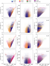 |
Fig. 4 Same as Fig. 3 but with the in situ component removed. |
| In the text | |
|
Fig. 5 Circular velocity curve of the four MW-like galaxies studied here. We note that the radii have been rescaled as explained in Section 2.1. The solar radius (R⊙ = 8.2 kpc) is indicated by the black vertical line. For comparison, we show the rotation curve of the MW measured by Eilers et al. (2019). |
| In the text | |
|
Fig. 6 Fraction of accreted stellar particles (ℱacc, solid lines) in the solar vicinity with velocities above a given threshold velocity (Vth), for the four simulated galaxies. The dashed lines show the evolution of the completeness of accreted stellar particles (𝒞acc) as a function of the threshold velocity. The vertical dashed line indicates a velocity threshold of 210 km s−1, used to kinematically define the halo in the solar vicinity. |
| In the text | |
|
Fig. 7 Distribution of the rescaled IoM parameters of the kinematically selected local halo sample of the four simulated galaxies (black contours). As a comparison, in each panel, the distribution of the local MW halo sample by L22 is shown by the red contours. In both cases the iso-density contours are plotted at the 1, 10, 20, 50, and 90% of the maximum density. |
| In the text | |
|
Fig. 8 Dendrogram (similar to Fig. 10 of L22) showing the relationship between the significant clusters detected by the single linkage algorithm according to their Mahalanobis distance in the IoM space, with the same cut-off threshold as used by D23 (indicated by the black line). For reference, the cut-off threshold used by L22 is shown by the dashed line. The vertical bars at the bottom of the figure indicate the relative contribution of the different progenitors to each significant cluster, using the same colour scheme as in Fig. 3. Note: the colours used to indicate the different groups of clusters linked together in the dendrogram are not related to the progenitors. |
| In the text | |
|
Fig. 9 Percentage of stellar particles, separated by their birth environment, located in the kinematically selected halo in the solar vicinity identified as being part of any significant cluster (>3σ) by the single-linkage method (upper panels). The lower panels show the similar quantity but considering only the particles that belong to clusters where their progenitor is the dominant contributor to a given clump. In all panels, the grey histograms indicate the contribution of each progenitor to the solar vicinity halo. Note: the second bar represent the value of all the accreted stellar particles grouped together. |
| In the text | |
|
Fig. 10 Median [Fe/H] (panels a), [Mg/Fe] (panels b), and stellar age (panels c) as a function of the mean (Lz) of each cluster found in the kinematically selected halo of the solar vicinity in the four simulated galaxies (circles). The circles are colour-coded by their fraction of accreted stellar particles. The triangles represent the same quantity, but with the in situ particles removed. The vertical dashed lines located at (Lz ± 500 km s−1 kpc−1) indicate the separations between the retrograde, non-rotating, and prograde clusters. For the prograde clusters, the metallicity, but mostly the [Mg/Fe] and the stellar age separate well those dominated by in situ and accreted particles. However, none of those parameters is able to disentangle the clusters dominated by in situ to those dominated by accreted particles for the non-rotating and the retrograde clusters. |
| In the text | |
|
Fig. 11 Fraction of accreted stellar particles in different area of the [Fe/H] vs [Mg/Fe] diagram for the retrograde, non-rotating, and prograde particles of the kinematically selected halo in the solar vicinity of the four simulated galaxies. In each panel, the red contour lines show the distribution of the 1, 25, 50, 75, and 90% distribution of the particles. |
| In the text | |
|
Fig. 12 Location in the IoM space of the grouped of clusters found in the kinematically selected halo in the solar vicinity of Au. 27 using the Mahalanobis distances. The colour scheme used is the same as for Fig. 8. The clusters that are not part of any group are shown in black. The background grey scale shows the density variation. |
| In the text | |
|
Fig. 13 Completeness and purity of the groups of clusters as a function of the Mahalanobis distance threshold (DM,th) chosen to group clusters together. For the purity, the solid lines represent the purity defined as the average cluster purity within groups (𝒫cg), while the dashed lines indicate the average purity of the groups (𝒫g). The threshold values used by L22 and D23 are indicated by the vertical dashed and solid lines, respectively. Note that the completeness and purity reported here only refer to the accreted progenitor. Stellar particles formed in situ are excluded (see Sect. 4.3). |
| In the text | |
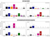 |
Fig. 14 Same as Fig. 9 but considering only the accreted particles. |
| In the text | |
|
Fig. 15 Same as Fig. 8 but for the solar vicinity sample, considering only the accreted particles for Au. 27. |
| In the text | |
|
Fig. 16 Confusion matrix of the KS test, comparing the MDF of each significant cluster found in Au. 27 considering only particles from accreted progenitors. The green cells indicate pairs of clusters sharing the same dominant progenitor and which have a similar MDF at the 95% confidence level (p-value >0.05, true positive). The red cells show pairs of clusters with a similar MDF but with different dominant progenitor (false positive). The grey cells show the pair of clusters with the same dominant progenitor but with different MDF at the 95% confidence level (false negative). The pair of clusters that are not dominated by the same progenitor and that have not the same MDF at the 95% confidence level (true negative) are shown by the white cells. As the matrix is diagonally symmetric, we decided to not colour code the cells in the lower part of the matrix for visibility reasons. The orange rectangles show the groups of clusters linked together by the Mahalanobis distance using the same cut-off value of D23. The clusters are ordered in the same way that in Fig. 8, with their reference ID. indicated in each row and column. |
| In the text | |
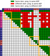 |
Fig. 17 Same as Fig. 16 but using the ADF instead of the MDF. |
| In the text | |
|
Fig. 18 Toy model illustrating the over- and under-dense regions in the IoM of an artificial halo (right panel) created by reshuffling the velocities of the original particles (left panel). In the original distribution, 1000 particles are on perfectly circular orbits and 100 particles on perfectly vertical orbits. In both panels, black lines delineate the possible distribution limits in energy-angular momentum, and the dashed line indicates the energy limit for a particle to be considered bound. |
| In the text | |
|
Fig. 19 Variation in the significance in the IoM of the originally kinematically selected halo in the solar vicinity of the BGM (upper panels) and of Au. 27 (lower panels) compared to the set of 100 artificial halos. In the lower row, the ellipses indicate the location of the significant clusters detected by the single linkage method using the in situ and accreted particles. |
| In the text | |
Current usage metrics show cumulative count of Article Views (full-text article views including HTML views, PDF and ePub downloads, according to the available data) and Abstracts Views on Vision4Press platform.
Data correspond to usage on the plateform after 2015. The current usage metrics is available 48-96 hours after online publication and is updated daily on week days.
Initial download of the metrics may take a while.