| Issue |
A&A
Volume 704, December 2025
|
|
|---|---|---|
| Article Number | A283 | |
| Number of page(s) | 23 | |
| Section | Planets, planetary systems, and small bodies | |
| DOI | https://doi.org/10.1051/0004-6361/202554329 | |
| Published online | 23 December 2025 | |
Sub-Jupiter gas giants orbiting giant stars uncovered using a Bayesian framework★
1
Instituto de Estudios Astrofísicos, Facultad de Ingeniería y Ciencias, Universidad Diego Portales,
Av. Ejército 441,
Santiago,
Chile
2
Centro de Astrofísica y Tecnologías Afines (CATA),
Casilla 36-D,
Santiago,
Chile
3
European Southern Observatory,
Alonso de Córdova 3107, Vitacura, Casilla
19001,
Santiago,
Chile
4
Instituto de Astronomía, Universidad Católica del Norte,
Angamos 0610,
1270709
Antofagasta,
Chile
5
United States Fulbright Fellow; Chile Fulbright Commission,
Chile
6
University of Southern Queensland, Centre for Astrophysics,
Toowoomba,
QLD
4350,
Australia
7
Facultad de Ingeniería y Ciencias, Universidad Adolfo Ibáñez,
Av. Diagonal las Torres 2640, Peñalolén,
Santiago,
Chile
8
Millennium Institute for Astrophysics,
Chile
9
Data Observatory Foundation,
Santiago,
Chile
10
Department of Physics & Astronomy, College of Charleston,
66 George Street
Charleston,
SC
29424,
USA
★★ Corresponding author: This email address is being protected from spambots. You need JavaScript enabled to view it.
Received:
28
February
2025
Accepted:
29
August
2025
Abstract
Giant stars have been shown to be rich hunting grounds for those aiming to detect giant planets orbiting beyond ~0.5 AU. Here we present two planetary systems around bright giant stars, found by combining the radial-velocity (RV) measurements from the EXPRESS and PPPS projects, and using a Bayesian framework. HIP 18606 is a naked-eye (V = 5.8 mag) KOIII star, and is found to host a planet with an orbital period of ~675 days, and to have a minimum mass (m sini) of 0.8 MJ and a circular orbit. HIP 111909 is a bright (V = 7.4 mag) K1III star, and hosts two giant planets on circular orbits with minimum masses of m sini=1.2 MJ and m sini=0.8 MJ, and orbital periods of ~490 d and ~890 d, for planets b and c, respectively, strikingly close to the 5:3 orbital period ratio. An analysis of the 11 known giant star planetary systems arrive at broadly similar parameters to those published, whilst adding two new worlds orbiting these stars. With these new discoveries, we have found a total of 13 planetary systems (including three multiple systems) within the 37 giant stars that comprise the EXPRESS and PPPS common sample. Periodogram analyses of stellar activity indicators present possible peaks at frequencies close to the proposed Doppler signals in at least two planetary systems, HIP 24275 and HIP 90988, calling for more long-term activity studies of giant stars. Even disregarding these possible false positives, extrapolation leads to a fraction of 25–30% of low-luminosity giant stars hosting planets. We find that the mass function exponentially rises towards the lowest planetary masses; however, there exists a ~93% probability that a second population of giant planets with minimum masses in the range 4–5 MJ is present, worlds that could have formed by the gravitational collapse of fragmenting protoplanetary disks. Finally, our noise modelling reveals a lack of statistical evidence for the presence of correlated noise at these RV precision levels, meaning white noise models are favoured for such datasets. However, different eccentricity priors can lead to significantly different results, advocating for model grid analyses such as those applied here to be regularly performed. By using our Bayesian analysis technique to better sample the posteriors, we are helping to extend the planetary mass parameter space to below 1 MJ, building the first vanguard of a new population of super-Saturns orbiting giant stars.
Key words: planets and satellites: detection / planets and satellites: dynamical evolution and stability / planets and satellites: formation / planets and satellites: fundamental parameters / planets and satellites: gaseous planets / planet-star interactions
Based on observations collected at La Silla – Paranal Observatory under programme IDs 085.C-0557, 087.C.0476, 089.C-0524, 090.C-0345, 097.A-9014, 0107.A-9004, 112.2666.001 and through the Chilean Telescope Time under programme IDs CN-12A-073, CN-12B-047, CN-13A-111, CN-2013B-51, CN-2014A-52, CN-15A-48, CN-15B-25 and CN-16A-13.
© The Authors 2025
 Open Access article, published by EDP Sciences, under the terms of the Creative Commons Attribution License (https://creativecommons.org/licenses/by/4.0), which permits unrestricted use, distribution, and reproduction in any medium, provided the original work is properly cited.
This article is published in open access under the Subscribe to Open model. This email address is being protected from spambots. You need JavaScript enabled to view it. to support open access publication.
1 Introduction
The study of planetary systems orbiting intermediate-mass stars, those with masses ≥1.5 M⊙, or evolved stars has mainly been carried out using the radial-velocity (RV) method (e.g. Johnson et al. 2007; Niedzielski et al. 2007; Wittenmyer et al. 2011; Jones et al. 2011; Ottoni et al. 2022). This may be surprising, given that large survey transit work from both the ground and space has recently given rise to an explosion of exoplanet detections. However, the dominant orbital architecture of these systems, coupled with the observational strategies we employ to discover and characterise them, renders the RV method the most efficient tool in this work. Firstly, stars with an effective temperature (Teff) hotter than around 6500 K, present few spectral lines with which to perform RV analyses, and therefore those more massive stars on the main sequence inhibit precision RV surveys. Hence, to gain RV access to the planetary systems orbiting those stars, it is necessary to observe them when they have evolved off the main sequence. At that point they cool down enough to present a rich forest of spectral lines that can be used to perform precision RV analysis. Furthermore, these studies have found a desert region between these stars and the first inner gas giant planet that orbits them, that reaches to around 0.5 AU (e.g. Sato et al. 2008; Jones et al. 2013). This means that there are very few gas giant planets orbiting close enough to their host star to transit, and since the transit probability is inherently low, few transiting worlds have been detected orbiting both massive stars on the main sequence and their giant star counterparts. However, those that have been detected (e.g. Lillo-Box et al. 2014; Jones et al. 2018; Saunders et al. 2025) have revealed interesting phenomena, such as radius re-inflation (e.g. Grunblatt et al. 2016), and represent an exciting benchmark sample that is rich for further study.
Gas giant planetary systems orbiting giant stars have been found to show some remarkable properties, both in the number density of planets and their orbital distribution. Beyond the aforementioned lack of planets orbiting giant stars, it has also been shown that these planets are found more often orbiting more metal-rich hosts (Johnson et al. 2010a; Reffert et al. 2015), similar to those orbiting main sequence (MS) stars (Fischer & Valenti 2005; Sousa et al. 2011; Jenkins et al. 2013). The overall planet fraction increases with increasing stellar mass, until around 2 M⊙ (Jones et al. 2016), and the fraction of giant planets orbiting evolved stars is high, around 10% (Wolthoff et al. 2022), and up to ~33% for low-luminosity red giant branch (RGB) stars (Jones et al. 2021). Therefore, these stellar systems are rich hunting grounds to search for giant planets.
With a high abundance of giant planets orbiting field giant stars in the solar neighbourhood (up to ~200 pc), we can study them in detail to better understand their orbital properties, which provides a window into the dynamic past of these planets, along with the formation histories of planets orbiting intermediate-mass stars on the MS. Since the distribution of giant planets orbiting giant stars has been primarily mapped out using precision RV studies, the orbital parameters and physical characteristics, such as planetary masses, are heavily dependent on the RV models employed. In the past decade, the RV community has moved towards searching the parameter space using more sophisticated tools, such as Markov chains and Bayesian statistics, or other tools, for example genetic algorithms, coupled with more complex correlated noise models such as Gaussian processes or moving averages (see e.g. Gregory 2007; Tuomi & Kotiranta 2009; Feroz et al. 2011; Ségransan et al. 2011; Jenkins & Tuomi 2014; Faria et al. 2018 and refs therein). These approaches have led to a significant improvement in the detection and extraction of genuine Doppler signals, particularly when combined with RV (quasi-)periodic variability induced by stellar phenomena, such as magnetic activity and stellar pulsations.
The simultaneous inclusion of stellar activity noise models in the search for Doppler signals can provide strong gains when dealing with Doppler signal confidence. In the past, more evolved K-type giant stars than those we studied in this work, have shown (quasi-)periodic signals that share Doppler-like properties. Stars such as Aldebaran, γDraconis, and 42 Draconis exhibit long-period RV signals that could be interpreted as having planetary origins (i.e. Döllinger et al. 2009; Hatzes et al. 2015, 2018). However, it seems these signals may have a stellar origin, with the exact physical phenomena still under debate (Reichert et al. 2019; Döllinger & Hartmann 2021). More expansive noise modelling coupled with Bayesian statistics can help shed some light on such issues, and in the future circumvent them.
For this work, we applied a Bayesian approach to search for new planets orbiting giant stars from a joint analysis of the RV time series data obtained by two giant star planet search programmes, the EXoPlanets aRound Evolved StarS (EXPRESS; Jones et al. 2011) and the Pan-Pacific Planet Search (PPPS; Wittenmyer et al. 2011) projects. We also reevaluated additional systems with previously published planet candidates to check their validity. We paid special attention to testing various models with different priors and correlated noise models, with the goal of arriving at the most appropriate statistical model to explain the data. The manuscript is therefore organised as follows. The observations, data reduction, and RV measurements are presented in Sect. 2. In Sect. 3 we present the host star properties. The RV analysis and Bayesian orbital fitting are presented in Sect. 4. The new discoveries and known planetary system tests are discussed in Sect. 5. We present the stellar activity analysis in Sect. 6; the results from the general analysis of the population of known RV planets orbiting giant stars from this project are found in Sect. 7. Finally, some discussion points and the summary are found in Sect. 8.
2 Observational data
High-resolution spectra from three separate instruments (UCLES, CHIRON, and FEROS) were taken for the two new giant stars presented in this work. The observations for both of these targets were acquired as part of the EXPRESS and PPPS surveys, representing an amalgamation of data from two separate independent projects. These two projects complement each other well, with samples that somewhat overlap, both having 37 stars in common, and a number of planetary systems have already been published using their combined datasets (e.g. Jones et al. 2016; Wittenmyer et al. 2016, 2017b; Jones et al. 2021). An additional 11 discovered planetary systems were also analyzed for this work, using RVs taken by the same three spectrographs, and used to better understand the population of planets orbiting low-luminosity giant stars. The RV observations obtained with instruments are described in the three subsections below.
2.1 UCLES data
The PPPS operated from 2009 to 2015 as a collaboration between Australia, Caltech, and the National Astronomical Observatories of China. It was a Southern Hemisphere extension of the established Lick & Keck Observatory survey for planets orbiting northern “retired A stars” (Johnson et al. 2006, 2007, 2010a, e.g.). All RV data from the survey were made available in Wittenmyer et al. (2020). Data from the PPPS and EXPRESS were also used to compute occurrence rates of stars orbiting low-luminosity giant stars in Wolthoff et al. (2022). We obtained observations between 2009 and 2015 using the UCLES high-resolution spectrograph (Diego et al. 1990) at the 3.9-meter Anglo-Australian Telescope (AAT). UCLES, now decommissioned, achieved a resolution of 45 000 with a one-arcsecond slit. An iodine absorption cell provides wavelength calibration from 5000 to 6200 Å. Precise RVs are determined using the iodine-cell technique as detailed in Butler et al. (1996). The photon-weighted midtime of each exposure is determined by an exposure meter. All velocities are measured relative to the zeropoint defined by the iodine-free template observation. The UCLES velocities are given in Tables 1 and 2.
2.2 Chiron data
We observed a total of ~50 EXPRESS targets with the CHIRON (Tokovinin et al. 2013) high-resolution fibre-fed spectrograph mounted on the 1.5 m telescope at the Cerro Tololo InterAmerican Observatory (CTIO), in Chile. For each of these targets, we collected typically 10–15 individual spectra, between 2011 and 2023. For the observations we used the slicer mode, which leads to a resolving power of ~80 000, and the I2 cell in the light-path, and we adopted typical exposure times between 3 and 10 minutes, depending on the stellar magnitude. The data reduction was performed automatically by the CHIRON reduction pipeline (Paredes et al. 2021) and the final velocities were computed using the I2 cell method (Butler et al. 1996), with the pipeline described in (Jones et al. 2017). The resulting RVs are listed in Tables 1 and 2.
HIP 18606 radial-velocity and spectral diagnostic measurements.
HIP 111909 radial-velocity and spectral diagnostic measurements.
2.3 FEROS data
We observed the EXPRESS targets with the Fiber-fed Extended Range Optical Spectrograph (FEROS; Kaufer et al. 1999) high-resolution spectrograph, mounted on the 2.2 m telescope, at La Silla Observatory, between 2010 and 2024. FEROS is equipped with a secondary fibre that was illuminated by a simultaneous ThAr lamp, to correct for the nightly drift. We have obtained between 10 and 15 spectra per star, and for the planet candidates we have collected further data, typically reaching up to ~20 epochs to characterise the planetary orbital parameters. The exposure times varied between ~2 minutes for the brightest targets to 10 minutes for the faintest ones in the sample, leading to a S/N per extracted pixel ≳100. The data were reduced with the CERES pipeline (Brahm et al. 2017), that also computes the stellar RV, while the activity indicators were computed with the pipeline presented in Jones et al. (2017).
3 Stellar modelling
For each of the stars in our sample, (the two new planetary systems we announce in this work and the 11 stars with previously detected planets), we employed a two-step approach to calculate the stellar parameters. Firstly, we made use of the stellar parameter estimates from the Spectroscopic Parameters and atmosphEric ChemIstriEs of Stars (SPECIES; Soto & Jenkins 2018) algorithm. Although initially developed for use on main sequence dwarf stars, with a catalogue of over 580 dwarf star parameters presented in Soto & Jenkins, a SPECIES parameter catalogue for all giant stars in the EXPRESS project was also developed by Soto et al. (2021). This is the catalogue from which we draw the values used in this work, and therefore we refer to those papers for the details of how SPECIES calculates the stellar parameters. We note, however, that the Teff, log g, and [Fe/H] are measured from equivalent width fitting of high-resolution stellar spectra, whereas additional bulk properties such as mass and radius make use of the Isochrones package (Morton 2015). We also make use of the calculated equivalent evolutionary points (EEPs; see Dotter 2016), which gives rise to the most likely position of the star in evolutionary space. The EEPs allow us to discretely sample late-time stellar evolution, placing our stars at the terminal age main sequence (TAMS), the tip of the red giant branch (RGBTip), the zero-age core helium burning (ZACHeB), or the terminal-age core helium burning (TACHeB).
The second method we employ for calculating bulk stellar parameters is by using the ARIADNE code (Vines & Jenkins 2022). ARIADNE is an open-source Python package designed to automatically fit the spectral energy distribution (SED) with several grids of atmospheric models in order to determine parameters such as Teff log g, and radius, among others. ARIADNE operates as follows: firstly, it searches for publicly available photometric data on the star, then the SEDs are modelled using dynesty (Speagle 2020) with four different grids, the BT-Settl set (Allard et al. 2012; Castelli & Kurucz 2004; Kurucz 1993), and Phoenix v2 (Husser et al. 2013), and finally all models are averaged using the model probabilities as weights through a Bayesian Model Averaging approach, obtaining a final set of bulk parameters for each star.
As priors, we used the values derived from the SPECIES analysis for the Teff log g, and [Fe/H]. The extinction prior is a uniform distribution from zero to the maximum extinction in the line-of-sight from the SFD galactic dust maps (Schlegel et al. 1998; Schlafly & Finkbeiner 2011). Finally, we take the distances from Bailer-Jones et al. (2021) as a prior for the distance. The final calculated properties for all stars are shown in Table F.1, and their positions on an HR-diagram in Fig. 1.
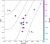 |
Fig. 1 HR diagram showing the position of all 13 target stars in this work (filled circles). The solid evolutionary curves were computed within the ARIADNE processing using MIST models, running between 1.0 M⊙ and 2.0 M⊙ and at a fixed solar metallicity. The colours of each of the data points corresponds to the stellar metallicity, with the colour scale shown on the right y-axis. |
4 RV modelling
To analyse all RV data, we make use of our Exoplanet Mcmc Parallel tEmpering Radial velOcity fitteR (EMPEROR) code version 1 (Vines et al. 2023; Peña Rojas & Jenkins 2025). EMPERORis an algorithm that is highly adapted to search for Keplerian signals in time series RV datasets. The code employs Markov chain Monte Carlo sampling, using the EMCEEpackage (Foreman-Mackey et al. 2017) to generate posterior samples for our targets. We employ the parallel-tempering routine within EMCEE, generating five chains with different temperatures, running from the coldest statistical chain, to progressively ‘hotter’ chains that ensure the full parameter space has been well sampled. Parallel-tempering is the process of raising the likelihood to some power (ℒβ, where β = 1/T, with T the temperature of the chain), such that narrow regions of high probability in the parameter space are broadened and damped across ever hotter chains. When considering the swap of states between chains, this process allows the cold chain (unmodified likelihood; β = 1) to move more easily throughout the parameter space of interest, guarding against being captured in non-global maxima of the posterior. In our case we set the short temperature ladder β to approximately {1.00, 0.49, 0.22, 0.11, 0.05}.
4.1 Bayesian formulism
Since EMPERORuses tempered Markov chains, we can make full use of Bayesian probabilities to manoeuvre the samplers to find and settle into the maximum of the posterior. We can also make use of the posterior probabilities once we locate the maximum to calculate the statistical probability of the model, or how favoured it is by the observed data. We can start with Bayes’ Theorem:
![Mathematical equation: $\[p(\boldsymbol{\theta} {\mid} D, M)=\frac{p(D {\mid} \boldsymbol{\theta}, M) p(\boldsymbol{\theta} {\mid} M)}{p(D {\mid} M)}.\]$](/articles/aa/full_html/2025/12/aa54329-25/aa54329-25-eq1.png) (1)
(1)
Here D is the observed data, θ is the parameter vector corresponding to model M, p(D|θ, M) is the likelihood distribution, p(θ|M) is the prior distribution, and the denominator p(D|Mi) = ∫ p (D|θi, Mi) p (θi|Mi) d θi is the marginalised likelihood of model Mi with parameters θi, which is also referred to as the Bayesian evidence, the quantity required such that the posterior integrates to unity over the parameter range.
The global model that we employ in this work is made up of a combination of seven terms and three nuisance terms. The form of the expression is
![Mathematical equation: $\[r_{i, j}=\gamma_j+\dot{\gamma_j t_i}+f_k\left(t_i\right)+\epsilon_{i, j}+\eta_{j, h}+\zeta_{j, q},\]$](/articles/aa/full_html/2025/12/aa54329-25/aa54329-25-eq2.png) (2)
(2)
where ri,j is the modelled RV for the i-th observation in the time series and j-th instrument, ![Mathematical equation: $\[\dot{\gamma}\]$](/articles/aa/full_html/2025/12/aa54329-25/aa54329-25-eq3.png) is a linear acceleration parameter per instrument as a function of time t to take care of any significant long-period trends in the data, and γj takes care of any offsets between the j-th instruments. ϵi,j is our white noise term that is the quadratic sum of the instrumental uncertainties, modelled as a zero mean normal distribution with a standard deviation equal to the measurement uncertainty (i.e.
is a linear acceleration parameter per instrument as a function of time t to take care of any significant long-period trends in the data, and γj takes care of any offsets between the j-th instruments. ϵi,j is our white noise term that is the quadratic sum of the instrumental uncertainties, modelled as a zero mean normal distribution with a standard deviation equal to the measurement uncertainty (i.e. ![Mathematical equation: $\[\mathcal{N}(0, \sigma_{i}^{2})\]$](/articles/aa/full_html/2025/12/aa54329-25/aa54329-25-eq4.png) ), and the excess stellar jitter noise, represented by a zero mean normal distribution with the standard deviation representing the jitter (i.e.
), and the excess stellar jitter noise, represented by a zero mean normal distribution with the standard deviation representing the jitter (i.e. ![Mathematical equation: $\[\mathcal{N}(0, \theta_{j i t}^{2})\]$](/articles/aa/full_html/2025/12/aa54329-25/aa54329-25-eq5.png) ). The ηj,h term represents the linear correlation functions for each instrument j that we introduce to model any additional noise that can be tracked by the measured h activity indicators, such as the chromospheric S-index or the bisector inverse slope (BIS). We note that the FWHM of the FEROS CCFs did not show any correlations or periodicities for any targets and so were not included. The form of these linear terms are given by
). The ηj,h term represents the linear correlation functions for each instrument j that we introduce to model any additional noise that can be tracked by the measured h activity indicators, such as the chromospheric S-index or the bisector inverse slope (BIS). We note that the FWHM of the FEROS CCFs did not show any correlations or periodicities for any targets and so were not included. The form of these linear terms are given by ![Mathematical equation: $\[\sum_{l} c_{l, i} l_{i, j}\]$](/articles/aa/full_html/2025/12/aa54329-25/aa54329-25-eq6.png) , with c being the correlation coefficient for each activity index l, normalised by its respective RMS. In reality, each of these stars has been preselected to represent likely RV stable stars (see Jones et al. 2011). For example, applying the expected RV pulsation amplitude scaling relations (Kjeldsen & Bedding 1995; Samadi et al. 2007; Kjeldsen & Bedding 2011), only three of the stars have pulsation amplitudes expected to be ≥10 m s−1, with the largest predicted value being ~20 m s−1. The estimated values as shown in Table F.1.
, with c being the correlation coefficient for each activity index l, normalised by its respective RMS. In reality, each of these stars has been preselected to represent likely RV stable stars (see Jones et al. 2011). For example, applying the expected RV pulsation amplitude scaling relations (Kjeldsen & Bedding 1995; Samadi et al. 2007; Kjeldsen & Bedding 2011), only three of the stars have pulsation amplitudes expected to be ≥10 m s−1, with the largest predicted value being ~20 m s−1. The estimated values as shown in Table F.1.
The ζj,q term relates to the correlated noise part, which we model using a moving average (MA) with exponential smoothing, given by
![Mathematical equation: $\[\zeta_{j, q}=\sum_q \phi_{j, q} exp \left(\frac{-\left|t_{i-q}-t_i\right|}{\tau_{j, q}}\right) m_{i-q, j},\]$](/articles/aa/full_html/2025/12/aa54329-25/aa54329-25-eq7.png) (3)
(3)
where q is the order of the MA, which in this work is fixed to unity to represent a first-order MA model. τ is the exponential smoothing parameter, the decay timescale of the correlation for a given instrument and MA order, and m represents the residuals of the model fit to the data. The final term in the global model expression is fk(ti), which represents the Keplerian component that is given by
![Mathematical equation: $\[f_k\left(t_i\right)=\sum_{n=1}^k K_n\left[\cos \left(\omega_n+\nu_n\left(t_i\right)\right)+e_n \cos \left(\omega_n\right)\right],\]$](/articles/aa/full_html/2025/12/aa54329-25/aa54329-25-eq8.png) (4)
(4)
which is a function that describes a k-Keplerian model with Kn being the velocity semi-amplitude, ωn is the longitude of pericentre, νn is the true anomaly and en is the eccentricity. νn is also a function of the orbital period and the mean anomaly M0,n, representing the phase (Θ) of the model function, a parameter we fit for.
By application of our model within the MCMC algorithm, at each step we must evaluate the probability of the proposal density, or the proposed new values for the parameter vector θ, and determine if the increase in probability warrants a selected movement of the chain within the hyper-dimensional space we are probing. Therefore, we require a description of the likelihood function p (D|θ, M) and a prior probability p (θ|M).
4.2 Likelihood function
Within EMPEROR we make use of a Gaussian likelihood function, which takes the following form:
![Mathematical equation: $\[\mathcal{L}(\theta)=p(D {\mid} \boldsymbol{\theta}, M)=\frac{1}{\sqrt{\operatorname{det} \mathbf{E}}} exp \left[-\frac{1}{2} \sum_{u \nu}\left(d_u-r_u\right)\left[\mathbf{E}^{-1}\right]_{u \nu}\left(d_\nu-r_\nu\right)\right].\]$](/articles/aa/full_html/2025/12/aa54329-25/aa54329-25-eq9.png) (5)
(5)
Here we have introduced E−1 as the inverse of the covariance matrix, implemented to take care of any correlated uncertainties we have in the data (d). For clarity we have set the subscripts u and v to be the positions within the matrix, columns and rows respectively. For fully independent uncertainties, the matrix itself is diagonal and this part of the expression simplifies to the χ2, being replaced with the term ![Mathematical equation: $\[\sum_{u} \frac{\left(d_{u}-r_{u}\right)^{2}}{\sigma_{u}^{2}}\]$](/articles/aa/full_html/2025/12/aa54329-25/aa54329-25-eq10.png) , where ru = ri,j, the different data points i and instruments j. Given that the likelihood is translated into log-space, we omit the constant term of 2πN/2 in the denominator outside of the exponential.
, where ru = ri,j, the different data points i and instruments j. Given that the likelihood is translated into log-space, we omit the constant term of 2πN/2 in the denominator outside of the exponential.
With the likelihood constructed as shown in Eq. (5), we require a kernel to fill out the positions of the covariance matrix, or model the correlations. In our case, and as shown in Eq. (3), we model the correlations using a first-order MA, meaning we only deal with the correlations two steps on either side of the diagonal, and the remaining positions in the matrix are set to zero. This serves to perform local smoothing of the data, whilst saving large fractions of computing time due to simpler matrix inversions.
4.3 Prior choice
In order to efficiently sample the RV data, we set the priors for our Bayesian probabilities to be similar to those we have utilised extensively in the past when searching for small signals in noisy data. Orbital period and RV amplitude are the two dominant parameters that define the success of the chain samplings to locate the maximum of the posterior. We set a wide uniform prior on both of these parameters, constrained to be three times the maximum time baseline of the RV data for the period, and three times the maximum spread in the RV measurements for the amplitude. The eccentricity is the only Keplerian parameter that is non-uniform, with it being set to a folded Gaussian function, centred at zero and with a standard deviation of either 0.1 (eTC) or 0.3 (eC), depending on the models. This effectively prioritises more circular orbits, which tend to be common outcomes of the planet formation and evolution process for giant star systems, yet it is flexible enough that planets on highly eccentric orbits are still allowed if the data strongly argue for their inclusion. In any case, we also test model sets with the eccentricity fixed to zero, representing purely circular orbital solutions (eF). The angular parameters for the Keplerian model are both uniform and set to the full extent between 0–2π radians. We tend to find that angular parameters are not very well constrained in many cases, particularly with circular, or close to circular orbits, and therefore flat priors are most appropriate here.
For the noise parameters, we again utilise mostly uniform prior bounds, such that we allow the most flexibility across the samplings, with one exception again, the jitter parameter. The offsets between the datasets (γ) are bounded to be between zero and the maximum of the RV measurement spread. The MA coefficients (ϕ) have a uniform prior between minus unity to unity, along with the linear acceleration parameter (![Mathematical equation: $\[\dot{\gamma}\]$](/articles/aa/full_html/2025/12/aa54329-25/aa54329-25-eq11.png) ), and the MA timescale (τ) is set to a fixed value of five days, which was arrived at after extensive testing across short and long timescales. Finally, the jitter parameter (θjit) maintains the normal distribution form as has been previously used with EMPEROR, yet we change the location of the mean to be set to 5 m s−1, since these giant stars are expected to have significant levels of p-mode-induced noise in RV data, at this level or more. We therefore also set the standard deviation to be 5 m s−1, allowing significantly higher values to be well sampled throughout the processing. All prior values and formats are listed in Table F.2.
), and the MA timescale (τ) is set to a fixed value of five days, which was arrived at after extensive testing across short and long timescales. Finally, the jitter parameter (θjit) maintains the normal distribution form as has been previously used with EMPEROR, yet we change the location of the mean to be set to 5 m s−1, since these giant stars are expected to have significant levels of p-mode-induced noise in RV data, at this level or more. We therefore also set the standard deviation to be 5 m s−1, allowing significantly higher values to be well sampled throughout the processing. All prior values and formats are listed in Table F.2.
5 New planetary system discoveries and known planet tests
We analyse the data employing various noise model approaches, assessing the model outcomes and best-fit probabilities when including or omitting MA correlated noise models, and/or linear activity correlation terms with the BIS measurements and S-activity indices from the FEROS spectra. Therefore, we run models with only white noise components (WNO models), a mixture of individual correlated noise components (BLCO or MA), combined linear activity components (BSLCO), or full correlated noise components (BLCMA and BSLCMA), giving rise to six separate model runs. We also run for fixed eccentricity and with the eccentricity as a constrained parameter, employing three different eccentricity priors for each of these models. The eccentricity priors are listed in Table F.2, with the ‘Tightly Constrained Eccentricity’ referring to the eTC prior, the ‘Constrained Eccentricity’ the eC prior, and the ‘Fixed Eccentricity’ the eF prior. We then compare the Bayes factors (BFs, parametrised as ΔBICs) between each of these models internally, (the same noise or eccentricity model but different numbers of Keplerian components), and externally, (comparing each best-fit model for different noise or eccentricity components), and we report the model that best describes the data.
5.1 HIP 18606
We model the 54 RVs for HIP 18606 without including any linear activity correlations, nor any MA correlated noise components in the first instance, meaning we are applying a pure white noise model approach at this time. We find a single statistically significant signal (BF > 5 or > 150× more probable than the next best model) with a period and amplitude of ![Mathematical equation: $\[674.94_{-6.28}^{+6.43}\]$](/articles/aa/full_html/2025/12/aa54329-25/aa54329-25-eq12.png) days and
days and ![Mathematical equation: $\[16.07_{-1.18}^{+1.12}\]$](/articles/aa/full_html/2025/12/aa54329-25/aa54329-25-eq13.png) m s−1, respectively, for the eF WNO model, which turns out to be the best fit (see Table F.4 for the BF values for each model). Including the BIS and S-index linear correlations without the MA components (BLCO & BSLCO models) also clearly detects the Doppler signal, and including the MA components in the model (MA, BLCMA, and BSLCMA) consistently find similar signals. We can see that the BLCO models have BIC values around 4–5 higher than the WNO models, whilst including the S-indices increases the BIC by a further 3–4, and then adding additional correlated components, (the MA models), increases the BIC by a further seven or more after that. The fact that the MA models are the least favoured models in general, tells us that there is a lack of noise correlations for this dataset, and so the simplest models better describe the velocity distribution for HIP 18606. No models across the three model sets found evidence of a second signal in the data.
m s−1, respectively, for the eF WNO model, which turns out to be the best fit (see Table F.4 for the BF values for each model). Including the BIS and S-index linear correlations without the MA components (BLCO & BSLCO models) also clearly detects the Doppler signal, and including the MA components in the model (MA, BLCMA, and BSLCMA) consistently find similar signals. We can see that the BLCO models have BIC values around 4–5 higher than the WNO models, whilst including the S-indices increases the BIC by a further 3–4, and then adding additional correlated components, (the MA models), increases the BIC by a further seven or more after that. The fact that the MA models are the least favoured models in general, tells us that there is a lack of noise correlations for this dataset, and so the simplest models better describe the velocity distribution for HIP 18606. No models across the three model sets found evidence of a second signal in the data.
Although the ensemble analysis is all in agreement with the existence of a single Doppler signal in the data, the solutions can be very different depending on which model set, or which type of eccentricity prior we employ. In this case, the models within the fixed eccentricity (eF) model set are highly favoured over the models that include eccentricity as a constrained parameter of the model (eTC & eC). For the WNO models, the eF model set provides a BIC that is ~8 lower than these other models. This trend is mirrored by the other models within each of these model sets, indicating that circular solutions are the most likely configurations that can explain the current data. Given that the eF models are less complex than the other model sets, the strong penalty on model complexity within the BIC could be biasing towards the selection of these circular models. However, interestingly, without correcting for the Chiron RV offset that appeared due to the full observatory shutdown throughout the recent global pandemic, the same signal is detected yet an eccentric solution is heavily favoured. This highlights the need to continuously understand instrument stability when properly modelling RV datasets, and also that the model selection will favour more complex eccentric solutions if the data argue for them. We rely on the calculated statistics and model complexity here to determine the best solution, and the bold eF WNO model is significantly favoured over all other models. When compared to its closest rival, the BLCO model within the same eF model set, the BF is found to be 4.5, which means a probability of 90× more in favour of the WNO model. The final full RV model and phase-folded RV curve are shown in Fig. 2, and the parameter estimates are found in Table F.3.
Since the search for additional companions in the RVs did not yield any confirmed candidates, we can therefore confirm the existence of a gas giant planet with a separation of just over 1.5 AU. No statistically significant linear trend is apparent in the data, meaning there is no current evidence in favour of any more massive companions at much larger separations than the time baseline of the data of a few thousand days.
5.2 HIP 111909
In the case of HIP 111909 when we fit the 52 RVs with all models, we find two statistically significant signals in all of them. In addition, for all models we find a 3rd signal in the data, yet this signal only has the same period in the eTC and eC model sets, and a different period in the eF model set. In fact, for a number of models we find a 4th signal that was statistically detected, yet the period of these were dependent on the model set assumed. For example, for the eC set the BLCO and MA models found signals with periods of ~435 days, whereas the fixed eccentricity set regularly found a fourth signal in the white noise only and bisector correlations only sets with a period of ~782 days. Since we did not find any agreement here for the 4th signal, we decided not to consider these as possible planets at this time, yet they are likely spurious noise related to poor model fitting for the k3 solutions we pick-up (see Table F.6). In the end, we decided to focus on the fact that all models across all sets detected three statistically significant signals in the data, and we discuss below which of these we can consider as detected planet candidates at this time.
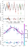 |
Fig. 2 RV analysis for HIP 18606. Top panel: RV time series for data taken with UCLES (blue circles), FEROS (red tilted triangles), and the pre- and post-pandemic Chiron data (orange and green triangles, respectively) for HIP 18606. The best-fit Keplerian model is represented by the black curve. Lower panel: RVs phase folded to the period of the detected planet candidate. The symbols represent the same data; however, the points are coloured depending on their observing date (see colour bar at right). The pink contours around the best-fit Keplerian model in black delimit the 1,2, and 3σ spread taken from the Markov chains. Both plots refer to the overall most probable model, the fixed eccentricity model with a white noise model component only. |
5.2.1 Two-planet solution only
Although we find excellent agreement for both signal parameters across all models for this dataset, we find a range of probabilities (BICs: 457–497). Following a similar pattern to the case of HIP 18606, the eTC model set provides slightly lower probability model fits than the eC model set, indicating models with slightly more flexibility should be favoured, yet the best fits are found to be for the circular models. We shall see this to be a recurring theme when looking at the rest of the stars we have analysed in this work, and hence eccentricity prior choice is important when searching for the ‘true’ model parameter values, even when the model choice is the same (i.e. a truncated Gaussian in this case, only the standard deviation is altered).
Another recurring theme we shall see is that the most probable set of models were found to be those without MA components for the eC and eF sets, with the overall best model the eF WNO model including two Keplerians (BIC=457.6). In general for this dataset, adding the MA correlated noise components only served to significantly increase the BIC values, even though the same two signals were detected. The best-fit planetary model finds two signals with periods of ![Mathematical equation: $\[487.08_{-3.63}^{+3.81}\]$](/articles/aa/full_html/2025/12/aa54329-25/aa54329-25-eq14.png) and
and ![Mathematical equation: $\[893.63_{-16.03}^{+14.89}\]$](/articles/aa/full_html/2025/12/aa54329-25/aa54329-25-eq15.png) days, and RV semi-amplitudes of
days, and RV semi-amplitudes of ![Mathematical equation: $\[25.57_{-1.52}^{+2.03}\]$](/articles/aa/full_html/2025/12/aa54329-25/aa54329-25-eq16.png) and
and ![Mathematical equation: $\[13.86_{-1.14}^{+1.25}\]$](/articles/aa/full_html/2025/12/aa54329-25/aa54329-25-eq17.png) m s−1, for planet candidates HIP 111909b and c, respectively.
m s−1, for planet candidates HIP 111909b and c, respectively.
The resulting solution we report here gives rise to the discovery of two giant worlds with minimum masses of 1.21±0.10 and 0.81±0.08 MJ, for planets b and c respectively. Their respective orbital periods are also intriguing, since the period ratio is found to be 1.84, very close to the 5:3 period ratio. In fact, they are just over 3σ away from this ratio, which hints at the possibility that these Jovian worlds were in or around the 5:3 mean motion resonance in the past, and were then possibly knocked out of resonance as the star evolved towards the RGB. Interestingly, dynamical tests provide hints that the planets are currently still in resonance, motivating further detailed dynamical studies to reveal if such a scenario is possible. We show the phase-folded RVs with best-fit Keplerians, along with the RV time series and best model, in Fig. 3, and the values for the signals drawn from this model are shown in Table F.5.
When looking at the excess noise, jitter, for the best-fit solution, we find that the jitter is significantly larger for the post-pandemic Chiron dataset, than when compared to the data taken prior to the observatory shutdown. Although this may seem drastic and could point to a change in the star’s activity status, or an instrumental issue with the Chiron spectrograph after reopening the observatory, we only have six RVs in the second Chiron set, and therefore it is most likely that this is just an issue of low number statistics.
5.2.2 Third detected signal
As mentioned, EMPEROR detected a 3rd statistically significant signal in all model sets and model runs. However, as the period of the 3rd of signal was not constant over all model sets, we decided not to report either of these as a true Doppler signal at this time, even though at least one of them may be. For the eTC and eC model sets, all models agree with the third signal having a period and amplitude of ~17.5 days and ~9 m s−1, respectively. For the eF model set, all models found a 3rd significant signal with a period and amplitude of ~41.5 days and ~10 m s−1, respectively. The amplitudes of the 3rd signal in all models agrees well, yet the eF model set consistently finds a 3rd signal that is nearly 2.5× larger than both the eTC and eC model sets, meaning there is no global agreement in the period of the 3rd signal as yet. A by-eye inspection of the phase-folded RV plots for both signals may indicate that the 17.5-day plot looks cleaner; however, the BIC is significantly better for the WNO eF model fit. We caution that if planets b and c are actually in resonance, any third signal could arise due to evolution of the orbital angles and would therefore require a full Newtonian model analysis to confirm its reality. Since the RV data does not statistically argue for any linear trend at this time, we are therefore left to conclude that HIP 111909 is orbited by at least two gas giant planets, with orbital periods relatively close to a 2:1 period ratio.
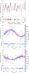 |
Fig. 3 RV analysis for HIP 111909. The top panel of the upper plot shows the full time series RV data, including data from the UCLES (blue circles), FEROS (red tilted triangles), and Chiron pre- and post-pandemic (orange and green triangles, respectively), along with the joint best-fit Keplerian model (black curve) for HIP 111909. The lower panel here shows the residuals to this model fit. The centre and lower plots show the phase-folded signals detected by EMPEROR, along with the best-fit models shown in black, and the 1, 2, 3σ uncertainty bounds (pink shaded regions). The lower panels highlight the residuals to the model fits. |
5.3 Known planet tests and additional candidates
In addition to the newly discovered planetary systems, we also tested our method on known systems to confirm this independent method also finds them, whilst searching for new signals. The 11 systems we studied were previously discovered using data from the UCLES, Chiron, and FEROS instruments, and we include here new spectroscopic data not used in the original papers. We report the BIC values from 18 different model tests per star in Appendix B. We also show the updated system parameters in Table F.7 and the RVs, both full time series and phase folded, along with the best-fit Keplerian models in Appendix C.
Overall, we find strong statistical evidence for the existence of these signals, as expected due to the reported high RV amplitude level of each (see Johnson et al. 2010b; Jones et al. 2015a,b; Wittenmyer et al. 2015; Jones et al. 2016; Wittenmyer et al. 2016, 2017b; Jones et al. 2021). However, our modelling tends to favour more circular orbits for a number of these systems where the eccentricity had previously been found to be statistically non-zero. Moreover, we also detect four new signals in this analysis, indicating the possible presence of additional planets orbiting the stars HIP 8541, HIP 67851, HIP 75092, and HIP 90988 (we elaborate more on these below). Finally, we confirm the linear trends for HIP 74890 (Jones et al. 2016) and HIP 90988 (Jones et al. 2021), and we detect statistically significant (beyond 99%) RV trends in HIP 67851, HIP 75092 and HIP 95124, providing strong evidence for additional long-period companions in these systems. In addition to giant planets orbiting within a few AUs, low-luminosity giant stars also appear to frequently host companions on much wider orbits.
6 Stellar activity analysis
6.1 Spectral index analyses
To allow the filtering of stellar activity signals that could impact the RV measurements, we extracted a number of spectral indices from the high-resolution spectral time series for each star. The indices we chose to make use of measure either the flux variations in spectral lines of interest or line shape variations in the form of asymmetries or width changes. For the flux variation indices, we make use of the classical chromospheric S-index (Duncan et al. 1991), and both the Hα and Na I D3 line indices (Santos et al. 2010). For the spectral line shape variations we choose to include the bisector inverse slope (BIS; Queloz et al. 2001) and the full width at half maximum (FWHM; e.g. Anglada-Escudé et al. 2016) of the CCF used to measure the RVs. These indices were used in three ways to study the activity, where (1) we analyse the indices using generalised Lomb-Scargle Periodograms (Zechmeister & Kürster 2009), (2) Keplerian fitting of the indices using standard manual cosine and Keplerian model fitting, and (3) by adding the indices into our EMPEROR Keplerian fitting prescription to model them simultaneously with the RVs, aiming to understanding their impact on the RVs directly. All GLS periodograms can be found in Appendix A, and therefore here we only discuss the four stars where there are potential activity signals that may relate to signals present in the measured RVs.
No stars in this sample showed any significant periodogram peaks in the line asymmetry indices that were found close to a planet candidate signal frequency. The activity indicators on the other hand did yield one such signal, and three others with weak peak powers that are close to planetary periods. HIP 18606, HIP 24275, HIP 90988, and HIP 95124 all have detected signals that could be flagged as potential false positives.
HIP 18606. In Fig. 4, we show the four periodograms for these stars, ranked from top to bottom in name ascending order. The top panel shows the periodogram of the S-index time series for HIP 18606, and this is the only statistically significant signal that crosses the 0.1% false alarm probability (FAP) limit and is relatively close to the detected planet candidate period. However, we can see that the peak frequency detected for this signal is ~146 days different from that of the planet candidate. We also ran an EMPEROR model of this time series (as in Rubenstein et al. 2025) and both the S-index signal and planet signal are statistically separated at the 17.9σ level. Therefore, we can safely rule out this activity signal as the culprit for the detected Doppler candidate signal in the RV time series.
HIP 24275. The second panel in Fig. 4 also shows the periodogram of the S-indices, but this time for the star HIP 24275. No peaks are statistically significant in this analysis, with the largest being found at a frequency of 6.9 days. However, a close second is the period that a manual fit to the time series gives as 912 days, which closely matches the candidate Doppler signal at 905 days. The EMPEROR results find a signal with a period of ![Mathematical equation: $\[883.8_{-38.9}^{+33.9}\]$](/articles/aa/full_html/2025/12/aa54329-25/aa54329-25-eq18.png) days; however, the model is rejected as it narrowly misses the statistical significance condition previously mentioned. The proximity of the EMPEROR signal in the S-indices to the RV signal might suggest that it is related to activity, though more data is needed to acquire any statistically significant result since there are only 11 epochs of data.
days; however, the model is rejected as it narrowly misses the statistical significance condition previously mentioned. The proximity of the EMPEROR signal in the S-indices to the RV signal might suggest that it is related to activity, though more data is needed to acquire any statistically significant result since there are only 11 epochs of data.
As mentioned, both of these planets were originally published in Wittenmyer et al. (2016) and our analysis above including activity modelling also did not remove this signal; therefore, we cannot definitively show that activity is driving the lower-frequency RV signal, but there exists the possibility that this is the case. Moreover, most of the models we ran (Appendix B) actually found three planet candidate signals, and even if the proposed planet c is found to be a false positive, additional data may yield a more definitive detection of a second planet at a period of around 290 days. No strong activity peaks are found in any of the periodograms for this star close to 290 days.
The first signal for this RV time series relating to the planet candidate b at a period of 550 days, appears to be sandwiched between the peak at 912 days and another around 430 days. The shorter period of these two signals also seems to be heavily asymmetric, which might mean there is a third peak hidden here that better matches the period of the planet b Doppler candidate signal, but we could not confirm that at this time, meaning more spectral data is needed to test if this is the case.
HIP 90988. The third panel in Fig. 4 shows the periodogram of the sodium (Na) D line time series for the star HIP 90988, again with no statistically significant signal as yet. However, the strongest peak closely matches the period of the previously detected planet b signal at ~452 days (Jones et al. 2021). In fact, the current data gives a peak period of 470 days from the periodogram, with a best-fit modelled signal period of ![Mathematical equation: $\[470.5_{-7.3}^{+6.3}\]$](/articles/aa/full_html/2025/12/aa54329-25/aa54329-25-eq19.png) days, which gives rise to a difference of only 2.4σ between the best-fit RV Doppler signal period and this activityinduced signal. Therefore, although both periods seem to be separated, they are not statistically distinct. Testing the planet candidate here with further data in the future is crucial, to ensure that the activity frequency is sufficiently well constrained and does not further approach that of the proposed planet. We also note that the second planet candidate at longer period, newly detected in this work, falls close to a small bump in the periodogram around 2560 days. In this case, the bump maximum is significantly lower than many other peaks at different frequencies, and cannot be interpreted as a potential activity-induced signal in the RV time series at this stage. Again, more spectral data will help to elucidate this issue.
days, which gives rise to a difference of only 2.4σ between the best-fit RV Doppler signal period and this activityinduced signal. Therefore, although both periods seem to be separated, they are not statistically distinct. Testing the planet candidate here with further data in the future is crucial, to ensure that the activity frequency is sufficiently well constrained and does not further approach that of the proposed planet. We also note that the second planet candidate at longer period, newly detected in this work, falls close to a small bump in the periodogram around 2560 days. In this case, the bump maximum is significantly lower than many other peaks at different frequencies, and cannot be interpreted as a potential activity-induced signal in the RV time series at this stage. Again, more spectral data will help to elucidate this issue.
HIP 95124. Finally, the fourth panel in Fig. 4 that relates to the periodogram of the Hα time series for the star HIP 95124, also shows the strongest statistical signal appearing close to the frequency of the detected planet b. The activity signal peak is found to be 656 days, whereas the planet signal is at 564 days, nearly 100 days separated. Additionally, when we run a best-fit model to the activity data we find an activity period that is more than 100 days separated from the planet candidate Doppler signal, and therefore it is unlikely to be the origin of the Doppler candidate. Furthermore, EMPEROR does not detect any significant signals in the Hα data, hence we conclude that HIP 95124b is likely a genuine planet orbiting this star.
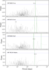 |
Fig. 4 Periodograms for four stellar activity indices that show peak powers close to a candidate planet signal detected for four of the stars in this sample. From top to bottom we show the S-activity index periodograms for HIP 18606 and HIP 24275, the Na I index for HIP 90988, and the Hα index for HIP 95124. The green vertical lines mark the positions of candidate planets and the horizontal blue dotted lines show the 0.1% false alarm probabilities. The periods of the strongest peaks are also labelled in each panel. |
6.2 ASAS photometric analysis
To further investigate whether stellar phenomena could be the source of the observed RV variations (e.g. Boisse et al. 2011), we analyzed the All Sky Automated Survey (ASAS; Pojmanski 1997) V-band photometry of all giant stars in this work. In order to ensure we are making use of the highest-quality datasets for these tests, we only used A- and B-grade ASAS data, which are known to be relatively free of various controllable sources of noise. Due to evidence of stability issues in the early photometric data, we calculated the mean and standard deviation of all data after JD 2452300. Using the statistics from the more stable data, we then applied a 3σ clipping filter to the entire baseline of the data, to remove serious outliers. This type of selection can also have the effect of removing data that were taken when the star was in another epoch of its activity cycle that is far from the norm, for example moments of extreme inactivity or extreme activity. However, this is also a desired effect since we are aiming to search for longer-term stable signals such as those from the star’s rotational frequency. In the top and middle panels of all plots in Appendix D we show the raw and cleaned data for each of our targets, and we can see that the majority of the removed outliers come from early in each time series, when the photometric quality was less stable.
After cleaning the ASAS data we again passed each dataset through a GLS periodogram analysis to search for any stable and statistically significant signals present in the time series, and we show all of these in the bottom panels of the figures in Appendix D. Only six of the sets showed statistically significant signals present in the data, with the rest showing nothing of interest. A few of these are attributed to signals arising due to the overall baseline of these discretely sampled time series, a common issue with periodogram analyses, whereas others seem to be genuine photometric frequencies found to be present on these stars at the time of the observations. However, what we were mostly interested in once again were the signals arising close to the frequencies of the planet candidates detected by the EMPEROR analysis. We show the three cases of interest that require discussion in Fig. 5.
The top panel in Fig. 5 shows the results for HIP 18606, which also was highlighted above in the spectral activity analysis of the S-index values. In fact, both the ASAS photometry and S-indices showcase a broadly similar pattern around the planet candidate frequency, with signal strength around 500–600 days. Here the photometry peak is closer to the RV signal period, although still not quite overlapping, with a period of 640.07 d. It should be noted that this power peak is not the maximum strength in the periodogram, but the third-highest frequency peak, below the 0.1% FAP. It also doesn’t quite match the peak frequency found in the S-indices, which was found at a significantly lower period, whereas the flanking peak at lower strength does match the S-index frequency. This may indicate that the S-indices are tracing stellar surface spot movements, at least at these frequencies.
The centre panel shows the results for HIP 24275, with the outer planet candidate RV signal falling in an area of increased power in the ASAS GLS periodogram. Indeed, this dataset also shows a weak peak in S-indices at the period of the proposed RV Doppler signal, and with the addition of this cluster of significant peaks surrounding the detected RV frequency, this casts serious doubt on the reality of HIP 24275c, likely indicating that this RV signal arises due to stellar surface phenomena and not an orbiting planet. The actual maximum is found to be at 1191 d; however, there are four statistically significant peaks surrounding the RV signal in this region, showing that the star presents an activity cycle, likely varying or multiple, at frequencies that are causing our algorithms to detect a signal in the RVs.
The bottom panel shows the GLS periodogram for the star HIP 56640, and although there are no statistically significant peaks at any frequency across the period space of interest, the largest peak corresponds to the period of the candidate Doppler signal in the RVs for this star.
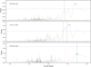 |
Fig. 5 GLS periodograms of the cleaned ASAS time series photometry for the stars HIP 18606, HIP 24275, and HIP 56640. The vertical lines mark the positions of the detected planet candidates in the RVs for each star, whereas the horizontal blue dashed lines represent the 0.1% FAP thresholds. The name of each target is also highlighted in the top left corner of each respective panel. |
6.3 Hipparcos photometric analysis
We also used the Hipparcos photometry (van Leeuwen 2007) to search for potential periodic signals in the data that could match the orbital period of the published and newly proposed planets. For this, we included only data with quality flag equal to 0 or 1, and we analysed the data in the same manner as the ASAS data, applying our GLS techniques to look for significant periodicities in the photometry. None were found for any of our sampled stars. In fact, only one periodogram showcased a small local peak close to a planetary candidate signal, that of HIP 74890. In Fig. 6 we show the data and periodogram, along with the position of the proposed planet. Visually there does appear overlap, yet statistically this does not appear to be the case. The photometric signal is found to peak at 762d, whereas the Keplerian period is 812d, significantly well separated given the uncertainties. We conclude therefore that Hipparcos photometry also does not rule out any proposed Doppler signals in our sample. All additional raw and cleaned Hipparcos photometeric time series, along with the GLS analyses, are shown in Appendix E.
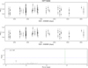 |
Fig. 6 Hipparcos photometric data for HIP 74890 is shown in the top panel. The middle panel shows the cleaned Hipparcos photometry for HIP 74890. The generalised Lomb–Scargle periodogram of the photometry is shown in the bottom panel. The horizontal line corresponds to the 0.1% (dotted blue) FAP significance level computed via 5000 bootstrap iterations on the photometry time series. The vertical green line represents the periods of the planets. |
7 General analysis results
Noise Properties. One of the general results from the analysis of these datasets is that the inclusion of a correlated noise model such as a moving average, is highly disfavoured when compared to more simple models that assume pure white noise only, or even simple linear correlations between the RVs and spectral line stability diagnostics such as bisector inverse slopes or the chromospheric S index. In the top panel of Fig. 7 we can see the distribution of the BFs for each of the noise models, following a violin plot format, and we find that the mean and spread increases as a function of model complexity. In addition, the density of these probabilities is highly condensed towards small values for the WNO models when compared to the other noise models, peaking towards BFs of zero. This illustrates well that for these low-luminosity giant stars, employing models that assume gaussian distributed noise only is generally a good approximation of the data. The other noise model distributions do not peak towards zero, but the position of their peaks also increase in BF with model complexity. Therefore, making use of more advanced analysis techniques for giant stars beyond periodograms, similar to those employed here, should focus more on properly sampling the posterior space to 1) constrain better the uncertainties and uniqueness of detected signals and 2) to detect new signals close to the intrinsic noise level of the data, rather than to model high-frequency noise correlations following frameworks that have successfully been applied to dwarf stars on the main sequence (e.g. Tuomi et al. 2013; Jenkins et al. 2013; Anglada-Escudé et al. 2016).
The high intrinsic noise level of these giant stars, commonly dubbed jitter, is one explanation for the lack of correlations in the measured RV noise. Additionally, the timescales of correlated noise may not be conducive to the RV sampling employed in surveys similar to EXPRESS. These stars generally rotate slowly (ν sin i~1–4 km/s) meaning they have long rotational periods and low expected activity induced signals from surface features such as spots, signals that are difficult to sample in a high-cadence RV survey. The sample has been selected to have B − V values below 1.2 to ensure RV stability (see Hekker et al. 2006), and this also doubles as a crude estimation of the coronal dividing line from (Haisch 1999), meaning they are expected to host hot coronas. However, hosting a hot corona can be independent of the activity level (Huensch & Schroeder 1996), and therefore these stars are still expected to exhibit relatively low photometric variability from effects such as rotating star spots (Henry et al. 2000). However, Henry et al. suggest that the variability that these stars show is driven primarily by non-radial pulsations, and from their Table 1 the periods are generally less than one month, (low-luminosity giants such as those here are expected to have periods of less than one day), with the main outlier showing a period of 240 days. Therefore, stars such as those with deep convective envelopes and large, extended atmospheres, could maintain pulsation frequencies that again work against a high-cadence RV survey. In the end, these types of RV surveys are biasing against potential correlated noise, aiding in the discovery of genuine Doppler signals from orbiting planets.
Eccentricity distribution. In the lower panel of Fig. 7, we show the same violin plot format, but for the BF values separated by the three different eccentricity priors we employed here. First of all, we can see that the tightly constrained prior, eTC, had a minimum that was higher than both the constrained prior, eC, and the circular fixed prior, eF, values, indicating it was the poorest choice overall. However, it has a more condensed appearance than the eF models, showcasing a lower spread across the BFs, in close agreement with the distribution of the eC models. This suggests that these models did not produce descriptions of the data as poor as those using the eF prior, and in general agreement with the eC prior models. We may have expected that the eTC and eC prior model sets would produce fairly similar results, and this indeed appears to be the case, with the eC model sets producing a similar overall distribution, but with slightly lower spread. Interestingly, the eF probabilities peak towards zero BF, highlighting that circular models generally explain the data better than models that allow for some non-zero eccentricity, even if that eccentricity is statistically similar to zero. Yet the distribution spread is generally broader around the lower BF values, it does not taper down towards the zero value, indicating that the circular models fit the data well but can be less constraining than the other two prior model sets.
Taking these results at face value, it appears that the gas giant planet population orbiting these types of giant stars, favour circular orbits in general. However, just as Sun-like dwarf stars on the main sequence do, they exhibit a population of massive companions whose orbits are significantly different from zero (e.g. Wittenmyer et al. 2017a; Jones et al. 2018; Bergmann et al. 2021), known as eccentric giants, even though in general their planets tend to be found on more circular orbits than the Sun-like population (Jones et al. 2014). In Fig. 8 we show the period-eccentricity distribution for the planets in the EXPRESS and PPPS samples, highlighting the populations of planets on circular orbits and the population of eccentric giants. In addition, we also find that our Bayesian formulism argues for the planets with eccentricities in close agreement with zero (i.e. e<0.2) to actually have circular configurations. Of all the 11 systems we analysed, the confirmed planets (red circles) are almost all exclusively on circular orbits, with only the one multi-planet system HIP 67851 showing significant non-circular orbits. We also show in the plot the mean and standard deviation (μ=0.11, σ=0.06) of the published eccentricities for these planets, which is the regime where the majority of planets are likely to reside on even more circular orbits, and we see they are less than two standard deviations away from zero. We can test the other planets in our samples (purple stars) in future works to see how many indeed favour circular orbits, but for the time being, these results are broadly consistent with the conclusions in Bowler et al. (2020), since the sub-population of long-period planets with eccentricities greater than 0.3 in this figure, contain a number of massive companions with a mean minimum mass of 8.5±7.2 MJ, with all three companions with minimum masses greater than 10 MJ being found in this parameter space.
Period – minimum mass distribution. All of the confirmed planets in this work have minimum masses in the range 0.3–5.0 Jupiter-masses, and orbital periods between 90–2800 days. To gain a better understanding of how our new discoveries and updated parameter estimates fit in the global picture of giant planetary systems, we show the distribution of planetary minimum masses as a function of orbital period in Fig. 9. We can see that the previously discovered planets that are represented by the red circles, all fall significantly above the 20 m s−1 sensitivity limit for a solar mass star, with the lowest-mass objects straddling the 2 M⊙ limit. This population of ‘low hanging fruit’ are expected to be the first set of planets uncovered, since their Doppler amplitudes are much higher than the instrumental sensitivity limits and the intrinsic stellar jitter (see Hekker et al. 2006). However, using our new method of better sampling the posterior parameter space, including more apt models for the RV data and including some additional RVs, the newly discovered planets marked by green diamonds fall mostly below this sensitivity limit. Actually, at the shortest orbital periods they reach down to the 10 m s−1 RV limit for a solar-mass star; however, we caution here that the two possible lowest-mass planet candidates are ringed to indicate that there is some evidence from the activity index analyses that these are related to stellar activity. Although the activity analysis for HIP 8541 did not yield any conclusive results, we note that the RV amplitude relating to planet candidate c is below that expected for the pulsations of this star from the empirical scaling relations.
HIP 67851 represents an interesting case since recent results from Fontanet et al. (2025) using data acquired with the Coralie spectrograph, (refer to that work for details on the observations), give rise to a significantly longer orbital period for planet c than is found using our independent dataset analysis (see Table F.7). This tension arises due to the poor sampling of the outer signal in our data, which is being constrained mostly by the two final RV points in the time series. Indeed, by including the Coralie data in our analysis, we find a much longer period planet, in good agreement with their published solution.
In addition to the newly constrained planet c solution, our analysis gives rise to a new planet candidate, HIP 67851d. The signal is found to have a frequency between those of planets b and c, existing outside of the inner 2:1 period ratio of planet c (see Fig. 10). Given there appears no indications of stellar activity affecting the RVs at this frequency, and none of our correlated noise models remove the signal, there is a strong probability that this arises from a real third gas giant orbiting this star. However, by performing a dynamical analysis of the system using the parameters shown in Table F.7 for the Coralie included data, we find that the system likely could not have such eccentric orbits. For the masses found, where all three are above a Jupiter-mass, only circular orbits at these periods are found to be stable. Anything non-circular causes rapid orbital evolution and the ejection of planet c. Statistically, circular orbits indeed describe the system well; however, more eccentric orbits are preferred. We do note that this could be affected by the process used in this work to constrain the previous Keplerian solution(s) when sampling for an additional one. The fact the eccentricities are constrained may present a small bias against finding better circular solutions, and so future work should be done to test this.
As for HIP 75092c, this would be the lowest-mass planet yet discovered by RV analysis orbiting a giant star, hosting a minimum mass of ![Mathematical equation: $\[0.33_{-0.03}^{+0.04}\]$](/articles/aa/full_html/2025/12/aa54329-25/aa54329-25-eq20.png) MJ. We draw caution here with the interpretation of this result, since 1) only when fixing the eccentricity prior to zero does this signal reach statistical significance, 2) there are two competing solutions at very similar, but distinct, periods, and 3) not all the models in the eF model set significantly detect this new signal. We note that all the models in all model sets arrive at the same k2 signal; however, the BFs never reach the ΔBF threshold of five to claim a statistical detection in those other cases. Therefore, more RV data is required to move forward with confidently calling this a newly detected low-mass planet. In any case, this population seems to trace out the real sensitivity limits of our data, as they rise in minimum mass towards the longest orbital periods we have sampled. This visually highlights the impact that detailed Bayesian modelling of the data can provide, opening up a new population of lower-mass planets orbiting giant stars without the need to wait many more years for significantly higher volumes of RV measurements to be acquired.
MJ. We draw caution here with the interpretation of this result, since 1) only when fixing the eccentricity prior to zero does this signal reach statistical significance, 2) there are two competing solutions at very similar, but distinct, periods, and 3) not all the models in the eF model set significantly detect this new signal. We note that all the models in all model sets arrive at the same k2 signal; however, the BFs never reach the ΔBF threshold of five to claim a statistical detection in those other cases. Therefore, more RV data is required to move forward with confidently calling this a newly detected low-mass planet. In any case, this population seems to trace out the real sensitivity limits of our data, as they rise in minimum mass towards the longest orbital periods we have sampled. This visually highlights the impact that detailed Bayesian modelling of the data can provide, opening up a new population of lower-mass planets orbiting giant stars without the need to wait many more years for significantly higher volumes of RV measurements to be acquired.
For the time being, it is difficult to draw any conclusions about the period-minimum mass distribution of giant planets orbiting these giant stars, particularly for this new population of lower-mass planets we have uncovered here. Given the limitations imposed by the RV sensitivity biases in the data, we can say that there does not appear to be a significant correlation between orbital period and planetary minimum mass, beyond the known lack of gas giants on short period orbits (<100 days or so). This new population of super-Saturns is too small to provide any first statements about their nature, even though they are appearing to populate a similar part of the parameter space as their more massive counterparts. In order to properly study the overall population, it is necessary to apply our Bayesian methodology to a much larger sample of these stars, and then statistically test to what level the RV biases are affecting our results, similar to the work of Tuomi et al. (2014) for lower-mass stars.
Mass function. It is interesting to explore the mass distribution of giant planets orbiting low-luminosity giant stars, particularly given that we are now beginning to uncover much lower-mass planets. In Fig. 11 we show a histogram of the normalised distribution of minimum masses, finding a strikingly similar form than what has been found for dwarf stars (e.g. Jorissen et al. 2001; Butler et al. 2006; Lopez & Jenkins 2012). The population is dominated by low-mass gas giants, those with minimum masses close to that of Jupiter. Indeed, there seems to be an abundance of Jupiter-mass planets, and then a significant drop in the frequency for planets above ~2 MJ, with a flat distribution above this value. Only a few examples of the highest-mass planets (the easiest worlds to detect with this method for a given orbital period) have currently been found.
If we compare this distribution to dwarf stars on the main sequence, we notice that a similar finding was also pointed out by Jenkins et al. (2017), who found an exponential function to be an excellent description of the data. The exponential model has the form
![Mathematical equation: $\[f(m)=A \times exp (-m ~sin (i))+B,\]$](/articles/aa/full_html/2025/12/aa54329-25/aa54329-25-eq21.png) (6)
(6)
where A and B are constants that were found through a Markov chain Monte Carlo analysis in that work, having values of 0.89±0.03 and ![Mathematical equation: $\[0.030_{-0.003}^{+0.004}\]$](/articles/aa/full_html/2025/12/aa54329-25/aa54329-25-eq22.png) , respectively, and are highlighted in the plot. Rather than fit a new exponential model to our distribution, given the fairly low number statistics, we overplot the distribution found by Jenkins et al. for the dwarf stars in Fig. 11 to test how well it describes the giant star sample. The functional form does a good job of describing the minimum mass distribution of these giant planets, especially considering the different normalisation factors for each sample. The RMS scatter around this model is found to be 0.05, after excluding the first bin that represents the lowest-mass planets and is heavily incomplete. Even including this bin only increases the scatter slightly, with a value of 0.07 found. Such a result argues in favour of a single formation mechanism at play for both dwarf and giant star planetary systems. Given that the progenitors of these giants were more massive than the typical solar mass dwarf star studies (mostly A and F stars that are expected to have more massive protoplanetary disk dust mass fractions; Pascucci et al. 2016) it is reasonable to assume that core accretion dominates planet formation across all stellar masses in the inner systems, with only the outcomes differing in absolute terms, such as more massive planets orbiting more massive stars for example.
, respectively, and are highlighted in the plot. Rather than fit a new exponential model to our distribution, given the fairly low number statistics, we overplot the distribution found by Jenkins et al. for the dwarf stars in Fig. 11 to test how well it describes the giant star sample. The functional form does a good job of describing the minimum mass distribution of these giant planets, especially considering the different normalisation factors for each sample. The RMS scatter around this model is found to be 0.05, after excluding the first bin that represents the lowest-mass planets and is heavily incomplete. Even including this bin only increases the scatter slightly, with a value of 0.07 found. Such a result argues in favour of a single formation mechanism at play for both dwarf and giant star planetary systems. Given that the progenitors of these giants were more massive than the typical solar mass dwarf star studies (mostly A and F stars that are expected to have more massive protoplanetary disk dust mass fractions; Pascucci et al. 2016) it is reasonable to assume that core accretion dominates planet formation across all stellar masses in the inner systems, with only the outcomes differing in absolute terms, such as more massive planets orbiting more massive stars for example.
Jenkins et al. (2017) discussed the existence of a pile-up of gas giant planets orbiting Sun-like stars with minimum masses above around 2 MJ indicating a break in the formation mechanism. Santos et al. (2017) went on to study this in a more statistical sense, finding that indeed there is observational evidence of two distinct planet populations, where super-Jupiters with masses greater than ~4 MJ tend to orbit more massive and more metal-poor hosts than lower-mass gas giants. In Fig. 11 we also see an emerging pile-up, or over-abundance of giant planets with minimum masses above 4 MJ.
In order to test if there is statistical evidence for a second population here, we ran a Hartigan-like Dip Test (Hartigan & Hartigan 1985). Assuming the exponential model is a good description of the unimodal observed distribution of planets, we compared the maximum deviation of the cumulative distribution function (CDF) of the observed data against the maximum deviation of the CDF from 1 M random realisations drawn from this model. The model CDFs were scaled to match the maximum of the observed empirical CDF to take care of observational bias. This allowed us to test to what extent the non-unimodality could appear due to random statistical fluctuations. We found a deviation greater than the observed distribution occurs in ~7% of cases, meaning there is a ~93% probability that there exists a second population of super-Jupiters orbiting these giant stars. Although this is not high enough to claim strong statistical significance at this time, by pushing towards 2σ it is highly suggestive.
As mentioned, the main sequence progenitors of the stars in the EXPRESS and PPPS samples were more massive than the typical Sun-like stars that make-up most dwarf star samples, and therefore we may expect the population of super-Jupiters to be more pronounced orbiting these stars, particularly the more metal-poor subset. However, of the 13 planets with masses of ~4 MJ or more discovered by these projects, only half of them orbit stars with sub-solar metallicities and of those half, only two are statistically separated from being in agreement with solar. This is indicative that stellar mass is the dominant factor in separating the possible two populations of giant planets orbiting nearby stars, with any metallicity effect being only secondary. Since a star’s mass is correlated with its protoplanetary disk dust mass by a positive power index (Andrews et al. 2013; Pascucci et al. 2016), this second population of giant planets could be the result of a separate formation/migration pathway, that of gravitational collapse of a heavily fragmented disk (e.g. Boss 1998; Stamatellos 2015). However, to place this on a more robust statistical footing a fully homogeneous Bayesian analysis of the RVs for all stars in these projects should be performed, along with a similar homogeneous analysis of the stellar metallicities to help remove all sources of bias. If this result holds, we can partition the population of gas giants into two based on their mass and formation channel, with Jupiters being formed through core accretion across all stellar masses from A–Ks, and super-Jupiters (>2~3 MJ) being formed through gravitational collapse of massive unstable protoplanetary disks.
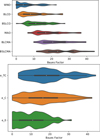 |
Fig. 7 Performance analysis of our modelling grids. Top panel: violin plot of the distributions of the Bayes factors (ΔBICs) compared to the best fit for all models applied to each of the four realisations of the noise tested in this work. The blue curve represents the WNO models, the orange curve highlights the BLCO models, the green curve shows the MAO models, and the red curve the BLC+MA models. Lower panel: violin plot of the distributions of the same Bayes factors, but separated by the three eccentricity priors that were tested in this work. The blue distribution is for the eTC prior, the orange distribution is for the eC prior, and the green distribution is for the eF prior. |
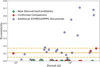 |
Fig. 8 Distribution of eccentricities of the giant planets within the EXPRESS and PPPS overlapping samples, as a function of their orbital period. The filled green diamonds represent the newly discovered planets in this work (including the possible candidates HIP 24275d and HIP 75092c for reference), the red circles highlight the additional confirmed planets, and the purple filled stars are all other planets from these projects not included here. The solid and dashed horizontal yellow lines mark the mean eccentricity of the 12 previously detected planets we include in this work and their associated 1σ uncertainty bounds, respectively. The ringed detections are those of HIP 24275b & d, HIP 75092c, and HIP 90988b, highlighted for the reasons discussed in the text. |
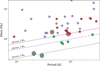 |
Fig. 9 Distribution of giant planet minimum masses as a function of orbital period discovered orbiting low-luminosity giant stars from the overlapping sample in EXPRESS and PPPS projects. As before, the filled green diamonds represent the newly discovered planets in this work, the red circles highlight the additional confirmed planets, and the purple filled stars are all other planets from these projects not included here. For reference, the 10 m s−1 and 20 m s−1 RV sensitivity limits for a 1 M⊙ star are shown by the dashed and dot-dashed curves, respectively, and the 20 m s−1 limit for a 2 M⊙ star is shown by the solid curve. The ringed detections are those of HIP 24275b & d, HIP 75092c, and HIP 90988b, highlighted for the reasons discussed in the text. |
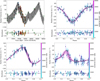 |
Fig. 10 The upper left plot shows the best fit Keplerian model (black curve) for the RV timeseries of HIP 67851, where the datasets shown are from UCLES (blue circles), FEROS (red triangles), Chiron (orange triangles), and Coralie (green triangles). The model residuals are also in the lower panel of the plot. The upper right plot and both lower plots show the phase-folded RVs for the first, second, and third planets detected in the system, respectively. The shaded pink regions mark the 1,2, and 3σ confidence boundaries around the model, and again the lower panels represent the residuals to the model fits. |
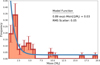 |
Fig. 11 Histogram showing the normalised frequency of giant planets orbiting low-luminosity giant stars, including those discovered in this work. The associated uncertainties are drawn from Poisson statistics based on the individual counts within each bin. The navy curve represents the exponential mass function proposed in Jenkins et al. (2017) for the giant planet sample orbiting lower-mass stars on the main sequence, with the model parameters are RMS scatter around this model, excluding the heavily incomplete bin, shown in the plot. The planet candidates HIP 24275b & d, HIP 75092c, and HIP 90988b have been included in this analysis. |
8 Discussion and summary
We have used precision RV data from the EXPRESS and PPPS giant star planet search projects to uncover two new nearby planetary systems, using a full Bayesian statistical approach on these types of stars. HIP 18606 and HIP 111909 have been found to host three gas giant planets between them, with a single planet found orbiting HIP 18606 on a 675 d orbit (HIP 18606b) and having a minimum mass of ~0.8 MJ. HIP 111909 on the other hand hosts two giant planets, both on long-period orbits, with HIP 111909b having an orbital period of nearly 500 d and HIP 111909c orbiting close to 900 d. The minimum masses of these two planets are in statistical agreement with that of Jupiter, adding to the large pantheon of Jupiter analogues orbiting stars that have recently evolved off of the main sequence and are called low-luminosity giant stars. The period ratio of the planets is strikingly close to the 5:3 resonance, and some short dynamical tests hint at the possibility that they are currently in resonance, although more detailed dynamical modelling in the future is required to confirm such a scenario.
In order to test the reliability and usefulness of combined Bayesian+MCMC approaches in the search for planets around giant stars, we also analysed 11 additional low-luminosity giants in order to confirm the reality of these detections, and to search for more planets in the systems. Our approach confirmed all of the currently known planets orbiting these stars, which means that our modelling confirmed that the signals are present. In addition, our activity index analysis, including new spectroscopic data, indicated that two signals could possibly be arising from stellar activity. In the case of HIP 24275, the S-indices show a peak in the periodogram at a period close to that of planet c. However, the peak is found at low significance, and based on only 11 data points. Similarly, a periodogram of the NaD indicators of HIP 90988 also reveals a peak close to the period of planet b, but again at low significance. We also found four new signals in the data, with the lowest amplitude of these possibly also originating from stellar activity; this takes the total number of planet candidates in this work to 20. When we analyse these planets in the orbital period versus minimum mass plane, we find that the low-mass cohort make up the first prototypes of a new population of super-Saturns that orbit these stars beyond 200 d orbital periods. HIP 75092c would be the lowest-mass planet yet discovered by RV analysis orbiting any giant star.
Our Bayesian approach revealed a detailed picture of the underlying characteristics of the planetary orbits. By statistically assessing models drawn from different eccentricity priors, we found that planets orbiting giant stars generally have circular orbits, indicating that the evolution of stars from the main sequence does not drastically affect widely separated giant planets. This would render them excellent samples to directly compare with planets on the main sequence orbiting lower-mass stars. The alternative is that their eccentricities are pumped throughout the stellar evolution off the main sequence, yet they quickly dissipate their orbital energy to return to circular orbits, possibly by interactions with other planets in the system. In such a scenario, it becomes more complicated to directly compare them with the main sequence sample, at least in a quantitative way. However, there is no global evidence as yet that this is indeed the case.
We were also able to test the mass function for these detected planets, and although the current numbers are somewhat small, an exponential function with values drawn from giant planet studies orbiting dwarf stars can explain the distribution well, albeit with a different normalisation factor. These results lend weight to the reality of the core accretion model of planet formation being at play, also in stars that are more massive than the Sun. This analysis also revealed an emerging pile-up of super-Jupiters with minimum masses of ~4 − 5 MJ, a result in agreement with previous works performed on more Sun-like dwarf stars. These results lend weight to the notion that there are two separate populations of gas giant planets, and that stellar mass, likely as a proxy for protoplanetary disk mass, is the dominant characteristic that drives this population bifurcation.
Our large grid of models told us that eccentricity prior width, not just the overall model, can be important when searching for true model parameters. If the prior is set too tight, the model does not have enough flexibility to search the wide parameter space efficiently, even if circular orbits are preferred. If the width is set too wide, the parameter estimates can be questionable, along with the potential loss of real signals. We also tested the usefulness of correlated noise models in these data, finding in general that white noise models do a better job of describing these types of RV datasets. Regardless of the eccentricity prior used, models with only white noise or with a BIS linear correlation applied were statistically favoured over correlated noise models that included moving averages. Therefore, random intrinsic variability of giant stars dominates over any correlated noise, at least at high frequency and with typical RV program sampling.
Finally, additional emerging candidate signals were detected in these datasets, particularly for HIP 111909, motivating the continued RV monitoring of these stars. The statistical significance of these candidates never crossed our detection threshold, although they were approaching relevance and were consistent across all models and model sets we tested. In the coming years with more RVs, new candidates will likely be detected that further enhance the reputation of low-luminosity giant stars as rich hunting grounds for massive worlds, but we must caution that long-term stellar activity modelling is also required to identify whether they are real or not. Even if we take the two previously announced planet candidates (HIP 24275c and HIP 90988b) that may be associated with activity index signals as being genuine false positives, then we could conclude that 12.5% (2/16) of Doppler candidates orbiting these types of stars are not real, dropping the fraction of giant planets orbiting low-luminosity giant stars by the same factor, and hence moving down to around the 25–30% level. In Vigan et al. (2021), the results presented from the direct imaging SHINE survey show that the fraction of widely separated (5–300 AU) substellar companions increases as a function of stellar mass, arriving at a value of ![Mathematical equation: $\[23.0_{-9.7}^{+13.5}\]$](/articles/aa/full_html/2025/12/aa54329-25/aa54329-25-eq23.png) % for BA-type stars. This is in good agreement with the value we have found here for at least a part of the parameter space that overlaps with our study. Since the stars studied in Vigan et al. are significantly younger than our sample and they reach out to much larger orbital separations, a hard comparison is beyond the scope of this work, but it is noteworthy that the results appear more than broadly consistent.
% for BA-type stars. This is in good agreement with the value we have found here for at least a part of the parameter space that overlaps with our study. Since the stars studied in Vigan et al. are significantly younger than our sample and they reach out to much larger orbital separations, a hard comparison is beyond the scope of this work, but it is noteworthy that the results appear more than broadly consistent.
Data availability
Appendices A, C, D, and E have been uploaded to the Zenodo website under the DOI 10.5281/zenodo.17024692, and can be found at the following link: https://zenodo.org/records/17024692. Tables 1 and 2 are available at the CDS via https://cdsarc.cds.unistra.fr/viz-bin/cat/J/A+A/704/A283
Acknowledgements
We acknowledge the traditional owners of the land on which the AAT stands, the Gamilaraay people, and pay our respects to elders past and present. We would like to thank the anonymous referee for their very thorough and helpful comments. J.S.J. gratefully acknowledges support by FONDECYT grant 1240738 and from the ANID BASAL project FB210003. R.B. acknowledges support from FONDECYT Project 1241963 and from ANID – Millennium Science Initiative – ICN12_009. C.A.G. acknowledges support from the National Agency for Research and Development (ANID) FONDECYT Postdoctoral Fellowship 2018 Project 3180668. MRD is supported by CONICYTPFCHA/Doctorado Nacional – 21140646, Chile. J.C. is supported by a grant from the SC Space Grant Consortium. M.T.P. acknowledges the support of Fondecyt-ANID fellowship ASTRON-0037.
References
- Allard, F., Homeier, D., & Freytag, B. 2012, Philos. Trans. Roy. Soc. Lond. A, 370, 2765 [NASA ADS] [Google Scholar]
- Andrews, S. M., Rosenfeld, K. A., Kraus, A. L., & Wilner, D. J. 2013, ApJ, 771, 129 [Google Scholar]
- Anglada-Escudé, G., Amado, P. J., Barnes, J., & et al. 2016, Nature, 536, 437 [Google Scholar]
- Bailer-Jones, C. A. L., Rybizki, J., Fouesneau, M., Demleitner, M., & Andrae, R. 2021, AJ, 161, 147 [Google Scholar]
- Bergmann, C., Jones, M. I., Zhao, J., et al. 2021, PASA, 38, e019 [Google Scholar]
- Boisse, I., Bouchy, F., Hébrard, G., et al. 2011, A&A, 528, A4 [NASA ADS] [CrossRef] [EDP Sciences] [Google Scholar]
- Boss, A. P. 1998, ApJ, 503, 923 [Google Scholar]
- Bowler, B. P., Blunt, S. C., & Nielsen, E. L. 2020, AJ, 159, 63 [Google Scholar]
- Brahm, R., Jordán, A., & Espinoza, N. 2017, PASP, 129, 034002 [Google Scholar]
- Butler, R. P., Marcy, G. W., Williams, E., et al. 1996, PASP, 108, 500 [Google Scholar]
- Butler, R. P., Wright, J. T., Marcy, G. W., et al. 2006, ApJ, 646, 505 [Google Scholar]
- Castelli F., Kurucz R. L., 2003, in Piskunov N., Weiss W. W., Gray D. F., eds, Modelling of Stellar Atmospheres, Vol. 210. Uppsala University, Uppsala, Sweden, p. A20 [Google Scholar]
- Diego, F., Charalambous, A., Fish, A. C., & Walker, D. D. 1990, SPIE Conf. Ser., 1235, 562 [NASA ADS] [Google Scholar]
- Döllinger, M. P., & Hartmann, M. 2021, ApJS, 256, 10 [CrossRef] [Google Scholar]
- Döllinger, M. P., Hatzes, A. P., Pasquini, L., et al. 2009, A&A, 499, 935 [NASA ADS] [CrossRef] [EDP Sciences] [Google Scholar]
- Dotter, A. 2016, ApJS, 222, 8 [Google Scholar]
- Duncan, D. K., Vaughan, A. H., Wilson, O. C., et al. 1991, ApJS, 76, 383 [Google Scholar]
- Faria, J. P., Santos, N. C., Figueira, P., & Brewer, B. J. 2018, J. Open Source Softw., 3, 487 [NASA ADS] [CrossRef] [Google Scholar]
- Feroz, F., Balan, S. T., & Hobson, M. P. 2011, MNRAS, 415, 3462 [Google Scholar]
- Fischer, D. A., & Valenti, J. 2005, ApJ, 622, 1102 [NASA ADS] [CrossRef] [Google Scholar]
- Fontanet, E., Udry, S., Ségransan, D., et al. 2025, A&A, 699, A38 [NASA ADS] [CrossRef] [EDP Sciences] [Google Scholar]
- Foreman-Mackey, D., Agol, E., Ambikasaran, S., & Angus, R. 2017, AJ, 154, 220 [Google Scholar]
- Gregory, P. C. 2007, MNRAS, 374, 1321 [NASA ADS] [CrossRef] [Google Scholar]
- Grunblatt, S. K., Huber, D., Gaidos, E. J., et al. 2016, AJ, 152, 185 [NASA ADS] [CrossRef] [Google Scholar]
- Haisch, B. M. 1999, in The Many Faces of the Sun: A Summary of the Results from NASA’s Solar Maximum Mission, eds. K. T. Strong, J. L. R. Saba, B. M. Haisch, & J. T. Schmelz, 481 [Google Scholar]
- Hartigan, J. A., & Hartigan, P. M. 1985, Ann. Statist., 13, 70 [CrossRef] [Google Scholar]
- Hatzes, A. P., Cochran, W. D., Endl, M., et al. 2015, A&A, 580, A31 [NASA ADS] [CrossRef] [EDP Sciences] [Google Scholar]
- Hatzes, A. P., Endl, M., Cochran, W. D., et al. 2018, AJ, 155, 120 [NASA ADS] [CrossRef] [Google Scholar]
- Hekker, S., Reffert, S., Quirrenbach, A., et al. 2006, A&A, 454, 943 [NASA ADS] [CrossRef] [EDP Sciences] [Google Scholar]
- Henry, G. W., Fekel, F. C., Henry, S. M., & Hall, D. S. 2000, ApJS, 130, 201 [Google Scholar]
- Huensch, M., & Schroeder, K. P. 1996, A&A, 309, L51 [Google Scholar]
- Husser, T. O., Wende-von Berg, S., Dreizler, S., et al. 2013, A&A, 553, A6 [NASA ADS] [CrossRef] [EDP Sciences] [Google Scholar]
- Jenkins, J. S., & Tuomi, M. 2014, ApJ, 794, 110 [NASA ADS] [CrossRef] [Google Scholar]
- Jenkins, J. S., Jones, H. R. A., Tuomi, M., et al. 2013, ApJ, 766, 67 [Google Scholar]
- Jenkins, J. S., Jones, H. R. A., Tuomi, M., et al. 2017, MNRAS, 466, 443 [Google Scholar]
- Johnson, J. A., Marcy, G. W., Fischer, D. A., et al. 2006, ApJ, 652, 1724 [Google Scholar]
- Johnson, J. A., Fischer, D. A., Marcy, G. W., et al. 2007, ApJ, 665, 785 [Google Scholar]
- Johnson, J. A., Aller, K. M., Howard, A. W., & Crepp, J. R. 2010a, PASP, 122, 905 [Google Scholar]
- Johnson, J. A., Howard, A. W., Bowler, B. P., et al. 2010b, PASP, 122, 701 [Google Scholar]
- Jones, M. I., Jenkins, J. S., Rojo, P., & Melo, C. H. F. 2011, A&A, 536, A71 [NASA ADS] [CrossRef] [EDP Sciences] [Google Scholar]
- Jones, M. I., Jenkins, J. S., Rojo, P., Melo, C. H. F., & Bluhm, P. 2013, A&A, 556, A78 [NASA ADS] [CrossRef] [EDP Sciences] [Google Scholar]
- Jones, M. I., Jenkins, J. S., Bluhm, P., Rojo, P., & Melo, C. H. F. 2014, A&A, 566, A113 [NASA ADS] [CrossRef] [EDP Sciences] [Google Scholar]
- Jones, M. I., Jenkins, J. S., Rojo, P., Melo, C. H. F., & Bluhm, P. 2015a, A&A, 573, A3 [NASA ADS] [CrossRef] [EDP Sciences] [Google Scholar]
- Jones, M. I., Jenkins, J. S., Rojo, P., Olivares, F., & Melo, C. H. F. 2015b, A&A, 580, A14 [NASA ADS] [CrossRef] [EDP Sciences] [Google Scholar]
- Jones, M. I., Jenkins, J. S., Brahm, R., et al. 2016, A&A, 590, A38 [NASA ADS] [CrossRef] [EDP Sciences] [Google Scholar]
- Jones, M. I., Brahm, R., Wittenmyer, R. A., et al. 2017, A&A, 602, A58 [NASA ADS] [CrossRef] [EDP Sciences] [Google Scholar]
- Jones, M. I., Brahm, R., Espinoza, N., et al. 2018, A&A, 613, A76 [NASA ADS] [CrossRef] [EDP Sciences] [Google Scholar]
- Jones, M. I., Wittenmyer, R., Aguilera-Gómez, C., et al. 2021, A&A, 646, A131 [EDP Sciences] [Google Scholar]
- Jorissen, A., Mayor, M., & Udry, S. 2001, A&A, 379, 992 [NASA ADS] [CrossRef] [EDP Sciences] [Google Scholar]
- Kaufer, A., Stahl, O., Tubbesing, S., et al. 1999, The Messenger, 95, 8 [Google Scholar]
- Kjeldsen, H., & Bedding, T. R. 1995, A&A, 293, 87 [NASA ADS] [Google Scholar]
- Kjeldsen, H., & Bedding, T. R. 2011, A&A, 529, L8 [NASA ADS] [CrossRef] [EDP Sciences] [Google Scholar]
- Kurucz, R. 1993, ATLAS9 Stellar Atmosphere Programs and 2 km/s grid, Kurucz CD-ROM No. 13 (Cambridge), 13 [Google Scholar]
- Lillo-Box, J., Barrado, D., Moya, A., et al. 2014, A&A, 562, A109 [NASA ADS] [CrossRef] [EDP Sciences] [Google Scholar]
- Lopez, S., & Jenkins, J. S. 2012, ApJ, 756, 177 [Google Scholar]
- Morton, T. D. 2015, isochrones: Stellar model grid package, Astrophysics Source Code Library [record ascl:1503.010] [Google Scholar]
- Niedzielski, A., Konacki, M., Wolszczan, A., et al. 2007, ApJ, 669, 1354 [NASA ADS] [CrossRef] [Google Scholar]
- Ottoni, G., Udry, S., Ségransan, D., et al. 2022, A&A, 657, A87 [NASA ADS] [CrossRef] [EDP Sciences] [Google Scholar]
- Paredes, L. A., Henry, T. J., Quinn, S. N., et al. 2021, AJ, 162, 176 [NASA ADS] [CrossRef] [Google Scholar]
- Pascucci, I., Testi, L., Herczeg, G. J., et al. 2016, ApJ, 831, 125 [Google Scholar]
- Peña Rojas, P. A., & Jenkins, J. S. 2025, A&A, in press, https://doi.org/10.1051/0004-6361/202554336 [Google Scholar]
- Pojmanski, G. 1997, Acta Astron., 47, 467 [Google Scholar]
- Queloz, D., Henry, G. W., Sivan, J. P., et al. 2001, A&A, 379, 279 [NASA ADS] [CrossRef] [EDP Sciences] [Google Scholar]
- Reffert, S., Bergmann, C., Quirrenbach, A., Trifonov, T., & Künstler, A. 2015, A&A, 574, A116 [NASA ADS] [CrossRef] [EDP Sciences] [Google Scholar]
- Reichert, K., Reffert, S., Stock, S., Trifonov, T., & Quirrenbach, A. 2019, A&A, 625, A22 [NASA ADS] [CrossRef] [EDP Sciences] [Google Scholar]
- Rubenstein, R. I., Jenkins, J., Peña, P., et al. 2025, A&A, 702, A139 [NASA ADS] [CrossRef] [EDP Sciences] [Google Scholar]
- Samadi, R., Georgobiani, D., Trampedach, R., et al. 2007, A&A, 463, 297 [NASA ADS] [CrossRef] [EDP Sciences] [Google Scholar]
- Santos, N. C., Gomes da Silva, J., Lovis, C., & Melo, C. 2010, A&A, 511, A54 [NASA ADS] [CrossRef] [EDP Sciences] [Google Scholar]
- Santos, N. C., Adibekyan, V., Figueira, P., et al. 2017, A&A, 603, A30 [NASA ADS] [CrossRef] [EDP Sciences] [Google Scholar]
- Sato, B., Toyota, E., Omiya, M., et al. 2008, PASJ, 60, 1317 [NASA ADS] [Google Scholar]
- Saunders, N., Grunblatt, S. K., Huber, D., et al. 2025, AJ, 169, 75 [Google Scholar]
- Schlafly, E. F., & Finkbeiner, D. P. 2011, ApJ, 737, 2 [Google Scholar]
- Schlegel, D. J., Finkbeiner, D. P., & Davis, M. 1998, ApJ, 500, 525 [Google Scholar]
- Ségransan, D., Mayor, M., Udry, S., et al. 2011, A&A, 535, A54 [NASA ADS] [CrossRef] [EDP Sciences] [Google Scholar]
- Soto, M. G., & Jenkins, J. S. 2018, A&A, 615, A76 [NASA ADS] [CrossRef] [EDP Sciences] [Google Scholar]
- Soto, M. G., Jones, M. I., & Jenkins, J. S. 2021, A&A, 647, A157 [NASA ADS] [CrossRef] [EDP Sciences] [Google Scholar]
- Sousa, S. G., Santos, N. C., Israelian, G., Mayor, M., & Udry, S. 2011, A&A, 533, A141 [NASA ADS] [CrossRef] [EDP Sciences] [Google Scholar]
- Speagle, J. S. 2020, MNRAS [arXiv:1904.02180] [Google Scholar]
- Stamatellos, D. 2015, ApJ, 810, L11 [Google Scholar]
- Tokovinin, A., Fischer, D. A., Bonati, M., et al. 2013, PASP, 125, 1336 [NASA ADS] [CrossRef] [Google Scholar]
- Tuomi, M., & Kotiranta, S. 2009, A&A, 496, L13 [NASA ADS] [CrossRef] [EDP Sciences] [Google Scholar]
- Tuomi, M., Jones, H. R. A., Jenkins, J. S., et al. 2013, A&A, 551, A79 [NASA ADS] [CrossRef] [EDP Sciences] [Google Scholar]
- Tuomi, M., Jones, H. R. A., Barnes, J. R., Anglada-Escudé, G., & Jenkins, J. S. 2014, MNRAS, 441, 1545 [Google Scholar]
- van Leeuwen, F. 2007, A&A, 474, 653 [CrossRef] [EDP Sciences] [Google Scholar]
- Vigan, A., Fontanive, C., Meyer, M., et al. 2021, A&A, 651, A72 [EDP Sciences] [Google Scholar]
- Vines, J. I., & Jenkins, J. S. 2022, MNRAS, 513, 2719 [NASA ADS] [CrossRef] [Google Scholar]
- Vines, J. I., Jenkins, J. S., Berdiñas, Z., et al. 2023, MNRAS, 518, 2627 [Google Scholar]
- Wittenmyer, R. A., Endl, M., Wang, L., et al. 2011, ApJ, 743, 184 [NASA ADS] [CrossRef] [Google Scholar]
- Wittenmyer, R. A., Wang, L., Liu, F., et al. 2015, ApJ, 800, 74 [NASA ADS] [CrossRef] [Google Scholar]
- Wittenmyer, R. A., Johnson, J. A., Butler, R. P., et al. 2016, ApJ, 818, 35 [NASA ADS] [CrossRef] [Google Scholar]
- Wittenmyer, R. A., Jones, M. I., Horner, J., et al. 2017a, AJ, 154, 274 [NASA ADS] [CrossRef] [Google Scholar]
- Wittenmyer, R. A., Jones, M. I., Zhao, J., et al. 2017b, AJ, 153, 51 [NASA ADS] [CrossRef] [Google Scholar]
- Wittenmyer, R. A., Butler, R. P., Horner, J., et al. 2020, MNRAS, 491, 5248 [NASA ADS] [CrossRef] [Google Scholar]
- Wolthoff, V., Reffert, S., Quirrenbach, A., et al. 2022, A&A, 661, A63 [NASA ADS] [CrossRef] [EDP Sciences] [Google Scholar]
- Zechmeister, M., & Kürster, M. 2009, A&A, 496, 577 [CrossRef] [EDP Sciences] [Google Scholar]
Appendix A Stellar activity index periodograms
This appendix is available on Zenodo at https://zenodo.org/records/17024692.
Appendix B Model posterior probabilities
HIP 8541 BIC values for the best-fit models for each of the examined model scenarios.
HIP 24275 BIC values for the best-fit models for each of the examined model scenarios.
HIP 56640 BIC values for the best-fit models for each of the examined model scenarios.
HIP 67851 BIC values for the best-fit models for each of the examined model scenarios, without the Coralie data.
HIP 67851 BIC values for the best-fit models for each of the examined model scenarios, with the Coralie data.
HIP 74890 BIC values for the best-fit models for each of the examined model scenarios.
HIP 75092 BIC values for the best-fit models for each of the examined model scenarios.
HIP 84056 BIC values for the best-fit models for each of the examined model scenarios.
HIP 90988 BIC values for the best-fit models for each of the examined model scenarios.
HIP 95124 BIC values for the best-fit models for each of the examined model scenarios.
HIP 114933 BIC values for the best-fit models for each of the examined model scenarios.
HIP 116630 BIC values for the best-fit models for each of the examined model scenarios.
Appendix C Radial-velocity analyses
This appendix is available on Zenodo at https://zenodo.org/records/17024692.
Appendix D ASAS photometric analyses
This appendix is available on Zenodo at https://zenodo.org/records/17024692.
Appendix E Hipparcos photometric analyses
This appendix is available on Zenodo at https://zenodo.org/records/17024692.
Appendix F Tables
Stellar properties.
Prior choices used in this work.
Most probable EMPEROR posterior mean RV model outcomes for HIP 18606
HIP 18606 posterior probability (p (θ|D, M) maxima for the best-fit models for each of the examined model scenarios.
EMPEROR posterior best RV model outcome for HIP 111909.
HIP 111909 posterior probability (p (θ|D, M) maxima for the best-fit models for each of the examined model scenarios.
EMPEROR orbital and physical parameters for the stars with known planets studied in this work, showing the results from the statistically favoured model only.
All Tables
HIP 8541 BIC values for the best-fit models for each of the examined model scenarios.
HIP 24275 BIC values for the best-fit models for each of the examined model scenarios.
HIP 56640 BIC values for the best-fit models for each of the examined model scenarios.
HIP 67851 BIC values for the best-fit models for each of the examined model scenarios, without the Coralie data.
HIP 67851 BIC values for the best-fit models for each of the examined model scenarios, with the Coralie data.
HIP 74890 BIC values for the best-fit models for each of the examined model scenarios.
HIP 75092 BIC values for the best-fit models for each of the examined model scenarios.
HIP 84056 BIC values for the best-fit models for each of the examined model scenarios.
HIP 90988 BIC values for the best-fit models for each of the examined model scenarios.
HIP 95124 BIC values for the best-fit models for each of the examined model scenarios.
HIP 114933 BIC values for the best-fit models for each of the examined model scenarios.
HIP 116630 BIC values for the best-fit models for each of the examined model scenarios.
HIP 18606 posterior probability (p (θ|D, M) maxima for the best-fit models for each of the examined model scenarios.
HIP 111909 posterior probability (p (θ|D, M) maxima for the best-fit models for each of the examined model scenarios.
EMPEROR orbital and physical parameters for the stars with known planets studied in this work, showing the results from the statistically favoured model only.
All Figures
|
Fig. 1 HR diagram showing the position of all 13 target stars in this work (filled circles). The solid evolutionary curves were computed within the ARIADNE processing using MIST models, running between 1.0 M⊙ and 2.0 M⊙ and at a fixed solar metallicity. The colours of each of the data points corresponds to the stellar metallicity, with the colour scale shown on the right y-axis. |
| In the text | |
|
Fig. 2 RV analysis for HIP 18606. Top panel: RV time series for data taken with UCLES (blue circles), FEROS (red tilted triangles), and the pre- and post-pandemic Chiron data (orange and green triangles, respectively) for HIP 18606. The best-fit Keplerian model is represented by the black curve. Lower panel: RVs phase folded to the period of the detected planet candidate. The symbols represent the same data; however, the points are coloured depending on their observing date (see colour bar at right). The pink contours around the best-fit Keplerian model in black delimit the 1,2, and 3σ spread taken from the Markov chains. Both plots refer to the overall most probable model, the fixed eccentricity model with a white noise model component only. |
| In the text | |
|
Fig. 3 RV analysis for HIP 111909. The top panel of the upper plot shows the full time series RV data, including data from the UCLES (blue circles), FEROS (red tilted triangles), and Chiron pre- and post-pandemic (orange and green triangles, respectively), along with the joint best-fit Keplerian model (black curve) for HIP 111909. The lower panel here shows the residuals to this model fit. The centre and lower plots show the phase-folded signals detected by EMPEROR, along with the best-fit models shown in black, and the 1, 2, 3σ uncertainty bounds (pink shaded regions). The lower panels highlight the residuals to the model fits. |
| In the text | |
|
Fig. 4 Periodograms for four stellar activity indices that show peak powers close to a candidate planet signal detected for four of the stars in this sample. From top to bottom we show the S-activity index periodograms for HIP 18606 and HIP 24275, the Na I index for HIP 90988, and the Hα index for HIP 95124. The green vertical lines mark the positions of candidate planets and the horizontal blue dotted lines show the 0.1% false alarm probabilities. The periods of the strongest peaks are also labelled in each panel. |
| In the text | |
|
Fig. 5 GLS periodograms of the cleaned ASAS time series photometry for the stars HIP 18606, HIP 24275, and HIP 56640. The vertical lines mark the positions of the detected planet candidates in the RVs for each star, whereas the horizontal blue dashed lines represent the 0.1% FAP thresholds. The name of each target is also highlighted in the top left corner of each respective panel. |
| In the text | |
|
Fig. 6 Hipparcos photometric data for HIP 74890 is shown in the top panel. The middle panel shows the cleaned Hipparcos photometry for HIP 74890. The generalised Lomb–Scargle periodogram of the photometry is shown in the bottom panel. The horizontal line corresponds to the 0.1% (dotted blue) FAP significance level computed via 5000 bootstrap iterations on the photometry time series. The vertical green line represents the periods of the planets. |
| In the text | |
|
Fig. 7 Performance analysis of our modelling grids. Top panel: violin plot of the distributions of the Bayes factors (ΔBICs) compared to the best fit for all models applied to each of the four realisations of the noise tested in this work. The blue curve represents the WNO models, the orange curve highlights the BLCO models, the green curve shows the MAO models, and the red curve the BLC+MA models. Lower panel: violin plot of the distributions of the same Bayes factors, but separated by the three eccentricity priors that were tested in this work. The blue distribution is for the eTC prior, the orange distribution is for the eC prior, and the green distribution is for the eF prior. |
| In the text | |
|
Fig. 8 Distribution of eccentricities of the giant planets within the EXPRESS and PPPS overlapping samples, as a function of their orbital period. The filled green diamonds represent the newly discovered planets in this work (including the possible candidates HIP 24275d and HIP 75092c for reference), the red circles highlight the additional confirmed planets, and the purple filled stars are all other planets from these projects not included here. The solid and dashed horizontal yellow lines mark the mean eccentricity of the 12 previously detected planets we include in this work and their associated 1σ uncertainty bounds, respectively. The ringed detections are those of HIP 24275b & d, HIP 75092c, and HIP 90988b, highlighted for the reasons discussed in the text. |
| In the text | |
|
Fig. 9 Distribution of giant planet minimum masses as a function of orbital period discovered orbiting low-luminosity giant stars from the overlapping sample in EXPRESS and PPPS projects. As before, the filled green diamonds represent the newly discovered planets in this work, the red circles highlight the additional confirmed planets, and the purple filled stars are all other planets from these projects not included here. For reference, the 10 m s−1 and 20 m s−1 RV sensitivity limits for a 1 M⊙ star are shown by the dashed and dot-dashed curves, respectively, and the 20 m s−1 limit for a 2 M⊙ star is shown by the solid curve. The ringed detections are those of HIP 24275b & d, HIP 75092c, and HIP 90988b, highlighted for the reasons discussed in the text. |
| In the text | |
|
Fig. 10 The upper left plot shows the best fit Keplerian model (black curve) for the RV timeseries of HIP 67851, where the datasets shown are from UCLES (blue circles), FEROS (red triangles), Chiron (orange triangles), and Coralie (green triangles). The model residuals are also in the lower panel of the plot. The upper right plot and both lower plots show the phase-folded RVs for the first, second, and third planets detected in the system, respectively. The shaded pink regions mark the 1,2, and 3σ confidence boundaries around the model, and again the lower panels represent the residuals to the model fits. |
| In the text | |
|
Fig. 11 Histogram showing the normalised frequency of giant planets orbiting low-luminosity giant stars, including those discovered in this work. The associated uncertainties are drawn from Poisson statistics based on the individual counts within each bin. The navy curve represents the exponential mass function proposed in Jenkins et al. (2017) for the giant planet sample orbiting lower-mass stars on the main sequence, with the model parameters are RMS scatter around this model, excluding the heavily incomplete bin, shown in the plot. The planet candidates HIP 24275b & d, HIP 75092c, and HIP 90988b have been included in this analysis. |
| In the text | |
Current usage metrics show cumulative count of Article Views (full-text article views including HTML views, PDF and ePub downloads, according to the available data) and Abstracts Views on Vision4Press platform.
Data correspond to usage on the plateform after 2015. The current usage metrics is available 48-96 hours after online publication and is updated daily on week days.
Initial download of the metrics may take a while.