| Issue |
A&A
Volume 704, December 2025
|
|
|---|---|---|
| Article Number | A141 | |
| Number of page(s) | 18 | |
| Section | Astronomical instrumentation | |
| DOI | https://doi.org/10.1051/0004-6361/202554541 | |
| Published online | 08 December 2025 | |
The Phase Induced Amplitude Apodizer and Nuller
High transmission, high dispersion coronagraphy at 2λ/D
1
Observatoire de Genève, Département d’Astronomie, Université de Genève,
Chemin Pegasi 51,
1290
Versoix,
Switzerland
2
Division of Space and Planetary Sciences, University of Bern,
Sidlerstrasse 5,
3012
Bern,
Switzerland
★ Corresponding author: This email address is being protected from spambots. You need JavaScript enabled to view it.
Received:
14
March
2025
Accepted:
26
August
2025
Abstract
Context. Proxima Cen b is the prime target in a search for life around a nearby exoplanet based on characterization of its atmosphere in reflected light. Due to its very high star-companion contrast (≤10−6), High Dispersion Coronagraphy is the most promising technique to perform such a characterization.
Aims. With a maximum separation of 37 mas, Proxima b can be observed with one of the VLT’s UT in the visible. This requires a coronagraph that provides high contrast (≤10−4) very close to the star (≤2 λ/D ) over a broad spectral range (∼30%)and with high transmission of the companion (≥50%). We searched for an optimal solution that benefits from the properties of single-mode fibers.
Methods. We introduce the Phase Induced Amplitude Apodizer and Nuller (PIAAN), a coronagraphic integral field unit, designed to feed a diffraction-limited spectrograph. It uses pupil remapping optics with moderate apodization combined with a single-mode fiber integral field unit. It exploits the properties of single-mode fibers to null starlight without reducing the companion coupling. The study focuses on a proper tolerance analysis and proposes a wavefront optimization strategy. A prototype has been built to demonstrate its performance.
Results. We show that the PIAAN can theoretically provide contrasts of 7 · 10−7 and a transmission of 72% at 2 λ/D over a bandwidth of 30%. We built and characterized a prototype and demonstrate the proposed wavefront control strategy. The prototype reached contrast levels of 3 · 10−5 over the full bandwidth, as expected from the tolerance analysis.
Conclusions. The new PIAAN coronagraph achieves performances that enable the study of exoplanets in reflected light. It is the main coronagraph candidate for the RISTRETTO instrument to observe Proxima Cen b on the VLT and its first technological milestone. It is also a solution of high interest for exploiting the spatial resolution and the large collecting area of future ELTs.
Key words: instrumentation: high angular resolution / instrumentation: spectrographs / methods: numerical / techniques: high angular resolution / techniques: imaging spectroscopy
© The Authors 2025
 Open Access article, published by EDP Sciences, under the terms of the Creative Commons Attribution License (https://creativecommons.org/licenses/by/4.0), which permits unrestricted use, distribution, and reproduction in any medium, provided the original work is properly cited.
This article is published in open access under the Subscribe to Open model. This email address is being protected from spambots. You need JavaScript enabled to view it. to support open access publication.
1 Introduction
We are at a pivotal moment in exoplanetary research, with the discovery of numerous Earth-like exoplanets. However, the detection and characterization of such a companion face significant challenges due to their close angular proximity to host stars and the brightness contrast between companions and stars.
High-contrast imaging techniques, supported by extreme qdaptive optics (XAO) systems, have enabled advancements in this field in the past decade. Instruments such as SPHERE (Beuzit et al. 2019), GPI (Macintosh et al. 2014), SCExAO (Jovanovic et al. 2015), and MAGAO-X (Males et al. 2024) use coronagraphs to suppress stellar light, allowing the faint signals of companions to be isolated. Other instruments improve contrast by exploiting differences in spectral lines caused by factors such as Doppler velocity shifts and molecular compositions (Sparks & Ford 2002; Snellen et al. 2015), with the support of XAO. The difference between the star and the companion spectra on the spectrograph can then potentially bring an additional 10−3 contrast gain after processing. It has already been demonstrated through the characterization pf giant exoplanet atmospheres, first with CRIRES (Snellen et al. 2014), or more recently with HiRISE (Vigan et al. 2024; Denis et al. 2025) for instance. High Dispersion Coronagraphy (HDC) aims at combining high resolution spectroscopy with high contrast thanks to an additional coronagraph. Coronagraphs are generally limited to a discovery zone beyond an inner working angle (IWA) of 3– 4 λ/D from the star, and are not fully exploiting the spatial resolving power of the largest telescopes available or to come. Instruments such as KPIC (Mawet et al. 2016) are now bridging the gap by allowing HDC down to 1 λ/D .
One of the current golden targets in exoplanet research is Proxima Cen b, an Earth-like companion orbiting in the habitable zone of the closest star to us. With a maximum apparent separation of 37 mas (i.e., 2 λ/D at λ=730 nm) and an estimated total contrast of 10−7, it is potentially observable with current 8m and 10 m telescopes using the HDC technique (Lovis et al. 2017; Blind et al. 2024). Obtaining such contrasts so close to the star requires using a XAO that delivers a Strehl ratio ≥70% in the visible and a coronagraph that provides a contrast ≤10−4 at a very small IWA ≤ 2 λ/D in the visible. The aforementioned instruments were not designed for this restricted and difficult parameter space, so a new instrument, RISTRETTO (Lovis et al. 2024), is being designed.
The Signal-to-Noise Ratio per absorption line of the HDC technique is written as (Snellen et al. 2015)
 (1)
(1)
where T is the total instrument transmission; F⊙ F⊕ are the flux from the host star and companion respectively; and ρ⊙ and ρ⊕ are the slit efficiency for the host star and the companion respectively. In the case of this paper, this corresponds to coupling into a single-mode fiber feeding the spectrograph. Finally, σdet is the noise from the detector (readout and dark). Considering observations limited by the stellar photon-noise, the SNR of HDC technique is proportional to
 (2)
(2)
where C = ρ⊙/ρ⊕ is the raw coronagraph or nuller contrast, at the slit or fiber injection level, as defined in Ruane et al. (2018a). Fig. 1 presents the expected SNR from Eq. 1 in the case of Prox Cen b on an 8-m telescope assuming a XAO providing S = 0.7, which appears as ρ⊕ = S × ρIFU in the figure. The figure shows the fundamental importance of the corona-graph transmission: Having a coronagraph with a transmission three times higher through ρ⊕ requires ten times shorter integration times. This gain also allows for an equal SNR for contrast requirements three to ten times lower in this regime. A higher transmission is therefore a fundamental advantage, as it relaxes the requirements over subsystems. A horizontal reading of the graph shows that the ultimate performance that can be expected from a coronagraph with ρIFU = 0.23 will be as good as a coronagraph with a transmission three times higher (ρIFU = 0.72) but with a ten times lower contrast, around 10−3. For a ground-based instrument, a higher transmission also presents a fundamental benefit on the XAO design, by relaxing Strehl and low-order performance requirements and by pushing the magnitude limit. With planet photons being scarce, we need a coronagraph that provides the highest throughput possible without compromising on contrast capabilities and while keeping in mind that the latter will be limited by XAO performance for a ground-based instrument. Coronagraphs with IWA ∼1–2 λ/D are notoriously difficult to design and operate due to tight tolerances to low-order aberrations, in particular tip-tilt jitter, that quickly degrade contrast. Since the XAO must provide diffraction-limited images, the use of single-mode fibers (SMF) is justified to feed the spectrograph. Such fibers have spatial filtering properties that can be exploited to cancel on-axis stellar light with a limited impact on the coronagraph transmission. A couple of such solutions, so-called nullers, are presented in Table 1. Among them, only the vortex fiber nuller (VFN) has been tested on-sky so far (Echeverri et al. 2019b), and it was strongly limited by the XAO performance, although its IWA is smaller than what we aim for in this study.
This paper presents the Phase Induced Amplitude Apodizer and Nuller (PIAAN), from concept to demonstration. Sect. 2 presents the concept, the theoretical solution, and an extensive tolerance analysis. Sect. 3 presents a wavefront control strategy, which is mandatory to face real-world operations and can be applied to other types of coronagraphic IFUs. In Sect. 4, we present our prototyping activities, our test setup, the characterization of the different parts, and finally a demonstration of the performance of the PIAAN.
2 Phase Induced Amplitude Apodizer and Nuller
2.1 Concept
The idea of the PIAAN is derived from speckle nulling techniques that exploit the spatial filtering properties of SMFs to cancel stellar light coupled into a fiber with a minimal transmission cost (Mennesson et al. 2006). In such fibers, the coupling efficiency, ρ, depends on the overlap integral between the SMF fundamental mode, Ef , and the electric field at focus, Eo, which is easily computed in the SMF far-field (Marcuse 1973):
 (3)
(3)
Here, Ef has a quasi-Gaussian shape that matches the core of an Airy point spread function (PSF), and ρ is maximized when the PSF is centered on the fiber. Otherwise, coupling is reduced, with some peculiar positions presenting a perfect null, i.e., ρ = 0. This generally happens when the fiber is between two diffraction rings or speckles, whose phases are opposite over the fiber mode and thus cancel each other in the overlap integral.
Coronagraphs such as SCAR (Por & Haffert 2020) and VFN (Ruane et al. 2018b) rely on this property to provide low stellar coupling ρ⊙ very close to a star, between 0.5 and 3 λ/D . This, however, comes with limited companion coupling, ρ⊕, and/or a small bandwidth.
The PIAAN is a coronagraphic integral field unit (IFU) similar to SCAR in its working principle, providing both high contrast and high transmission at a separation of 1.5–2.5 λ/D . It uses two main components:
PIAA optics that only weakly apodize the pupil (conversely to the original design in Guyon et al. 2005), generating a PSF with rings of lower amplitude and higher frequency. Compared to a standard VLT PSF, the rings are 10–40 times fainter, and two to three times more numerous.
An IFU made of seven hexagonal lenslets feeding seven SMFs.
Because the phase changes sign at every consecutive diffraction ring in the focal plane, the rings cancel each other efficiently over the fiber mode, allowing nulls ρ ∼ 10−5 − 10−6 (Fig. 2, top). This also enhances the bandwidth and improves the robustness to wavefront error, the tip-tilt jitter in particular.
Another property of the PIAA optics is to increase the match between the SMF mode and PSF core. While for a VLT, ρ ≤ 70% in absence of aberrations (Ruilier 1998), the PIAA potentially allows to reach ρ = 100% by removing the diffraction rings and concentrating light into a Gaussian core (Jovanovic et al. 2017). This benefit, however, is valid only if the fiber is placed on the PIAA optical axis. Due to the non-linear phase transformation, off-axis objects quickly get aberrated with a coma-like distortion (corresponding to the transformation of the tip-tilt phase by the PIAA), finally degrading ρ⊕. The degradation can be very fast, since 1 λ/D tip-tilt corresponds to 2π phase. In the case of the PIAAN, the weak apodization leads to less distortion, degrading the off-axis Strehl by about 15%, so that the coupling is still high at 2 λ/D (Fig. 2, bottom).
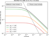 |
Fig. 1 Expected SNR for a Proxima Cen b observation on a VLT as a function of contrast for different coronagraph transmissions at 2λ/D. We assumed a total optical transmission of 5% (excluding the corona-graph transmission), a Strehl ratio of 70%, and σdet = 6e− for a reduced pixel in 1h of exposure time (Lovis et al. 2017). |
List of coronagraphic nuller concepts.
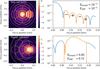 |
Fig. 2 Working principle of the PIAAN. Top: coupling of the star (on-axis). Bottom: coupling of the companion at 2 λ/D . Left: PIAA PSF and overlayed IFU at 620 nm, with the “companion” lenslet showcased. Right: horizontal cut view of the PSF in log scale, with the yellow part showing the electric field coupled to the fiber at the companion position. |
2.2 Model
The PIAAN is simulated using the Hcipy Python library (Por et al. 2018), from telescope to fiber coupling. The PIAA transformation and optical surfaces are computed based on ray-tracing and energy conservation principles (Guyon et al. 2005). We first developed a purely geometrical model, where we compute and apply the desired Gaussian apodization of the electric field (including a reduction in the secondary obstruction). Using entrance and exit rays coordinates, we build a function that remaps the entrance phase according to the PIAA transformation. This model is equivalent to considering an infinitely thin optics, neglecting physical propagation between surfaces. This model offers pretty fast computation speed and was therefore used for the global parametric exploration of Sect. 2.3. A scheme of this model is shown in Fig. 3.
We also developed a physical model to properly design and study real optics. Sag of each optical surface is extrapolated from the geometrical ray tracing, and Fresnel propagation is used between surfaces. We considered three possible configurations: a set of two mirrors as in the original paper (Guyon et al. 2005); a set of two flat-aspherical refractive optics as is more commonly done nowadays; and a novel aspherical-aspherical refractive optics (so-called rod optics). We only considered CaF2 glass, whose chromatism is also taken into account in the propagation.
One of the main limitations to producing such an optics is the minimum curvature radius achievable by the diamond turning tools. In this sense, the rod design presents the drawback of requiring sag and curvature radii six to seven times higher than the mirror one, or 1.5 times higher than a double lens design on the first surface, which present the strongest deviation. On the other hand, the design offers a proportionally lower sensitivity to sag and manufacturing errors, leading to a higher optical quality. Another advantage is that the optics does not require internal alignment, which proved to be advantageous. For our solutions, the physical model requires at least 600 pixels across the pupil to sample well the optical phase transformation at λ=600 nm. Computation time for seven fibers at a single wavelength is on the order of 1 to 2 seconds on a standard laptop.
Apart from the PIAA, the wavefront is generally propagated with a Fraunhofer propagator. Fresnel propagation is nevertheless used for tolerancing purposes or when a more accurate model can be implemented (e.g., for the microlens array) in order to study the potential impact of Talbot effects, etc. Aberrations can be injected in the pupil (e.g., atmospheric turbulence) or outside of it (e.g., lenses) to evaluate the performance in real conditions or to study wavefront control strategies and performance. Various defects on the IFU have also been implemented, i.e., independent near- and far-field misalignments to every lenslet.
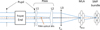 |
Fig. 3 Schematics of the PIAAN simulation. The front-end part is used to inject residual XAO phase screen and to simulate an optical relay with realistic optics and off-pupil aberrations. The MLA can be simulated with data from manufacturers if required. |
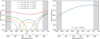 |
Fig. 4 Expected performance for a PIAAN optimizing detection of a companion at 2 λ/D with a 30% bandwidth, i.e., in the RISTRETTO case between 620 and 840 nm. Behavior outside the optimization band is shown in the light gray areas. Left: star null ρ⊙, showing the influence of the residual secondary obstruction. Right: companion coupling mostly independent of the residual obstruction. |
2.3 Optimization
The performance of the PIAAN depends on four main parameters:
PIAA apodization – An aggressive PIAA design can theoretically attenuate diffraction rings to 10−10 contrast level (Guyon et al. 2005), not requiring nulling at all. Such solutions, however, are not yet feasible or too complex to design. A sweet spot exists with a weak apodization, which generates a set of faint and high frequency rings that produce some null over SMFs. We investigated different apodization shapes (Gaussian and prolate mostly), but could not observe significant differences between best solutions, and decided to stick to the simple Gaussian one.
Central obstruction filling factor – A higher telescope central obscuration leads to stronger diffraction rings close from the PSF core. The PIAA is therefore also optimized to fill the secondary obstruction. Fully removing it leads to better performance, while keeping it higher than 0.05 Dtel severely limits the performance (Fig. 4, left).
Lenslet size and focal ratio – The lenslet constitutes a spatial filter in the focal plane and is used to optimize primarily the null level. With new 3D printing technologies, different lenslet shapes can be considered on the external ring. However, simulation with hexagonal and semi-circular lenslets led only to marginal differences, so we did not explore shape further. For the rest of the paper, we only consider hexagonal lenslets. Also note that the lenslet size or focal ratio must be adapted to the PIAA apodization, since the beam compression generates a non-linear magnification at the focal plane.
Lenslet focal lens – It mostly optimizes coupling of the companion, but allows some fine tuning of the null level. In practice, we converge to f-number values very close from the optimal for coupling the companion efficiently.
The optimization has been performed with the geometrical model via a simple grid exploration over the 4 parameters, with the largest exploration on the apodization strength and lenslet size, the main contributors to the performance. The best solutions are optimized for providing the highest SNR in the observation regime limited by the stellar photon noise, i.e., by maximizing Eq. (2), over a bandwidth of 30%. We also only consider here a VLT pupil, which does not have an impact on the results with the geometrical model.
We note that we can consider coupling the focal plane to the far-field or near-field of the SMF. Because the SMF mode field diameter is proportional to wavelength, just as with the diffraction limit PSF, it is generally better to perform near-field coupling to maintain high coupling over a broad range. However, when the focal plane is filtered by a lenslet, this is no longer true. With a lenslet size of 2 λ/D , near- and far-field coupling options perform nearly in the same way. Since in practice, it is easier to couple to far-field, this is the only solution considered in the rest of the paper.
Figure 4 presents the performance of the best solution, providing ⟨ρ⊕⟩ = 72% transmission at 2 λ/D, and stellar nulling ρ⊙ ≤ 10−5 at all wavelengths in the 30% bandwidth (or even ρ⊙ ≤ 10−6 for bluer wavelength for a slight cost in transmission), and an average of ⟨ρ⊙⟩ = 7 · 10−7. On the red side of the design band, contrast remains high, but SMF cut-off wavelength is soon reached. We did not study the case of endlessly single-mode photonic fibers. On the blue side, contrast degrades due to the central lobe extending into the lenslet. We show in Fig. 5 the influence of the apodization factor on the performance around the optimum solution. We observe in particular the rapid increase in off-axis aberration (plus, to a lower level, the increasing PIAA magnification), degrading ρ⊕ for FWHM ≤ 0.8Dtel, while the star nulling also starts to degrade. Note that the solution at FWHM= 0.5Dtel is already very aggressive in manufacturing, with minimum curvature radius 10 times smaller than our optimum solution.
It is well known that such coronagraphs have very tight tolerances, especially regarding a low-order wavefront error (Sect. 2.5). For all configurations, we also performed a first tolerance analysis over the first ten Zernike modes, to check whether a configuration or parameter improved technical feasibility of the coronagraph or could even relax XAO requirements. We only observed that solutions achieving better nulls are slightly more tolerant, but at a marginal level.
Figure 6 presents the transmission map of the PIAAN. The off-axis coupling is only 85% from the central fiber due to the off-axis aberration. As expected from SMF, the transmission drops quickly if the object is not centered, with a 50% loss at ±0.5 λ/D (±9 mas for a VLT in the visible). If the companion falls between 2 spaxels, transmission drops nearly to 0 due to the mode mismatch resulting from the spatial filtering by the lenslet (Fig. 6, cuts B and C). Since the position of the companion is not necessarily known, two exposures are required to homog-enize the transmission, with the IFU rotated by 30°. This can be accounted for as a transmission loss of 50% due to the double integration time. The same argument and strategy holds for a spaxel with lower performance: a spaxel with 0 transmission would account for 1/6 transmission loss with proper observing strategy. There is therefore a strong interest in determining where the companion is by other means, to place it directly on the best spaxel, and even to optimize the PIAAN working point for it.
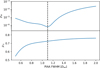 |
Fig. 5 Influence of the PIAA apodization on the PIAAN performance. The coupling is averaged for a 30% bandwidth. The optimal solution is shown with the dashed line. |
2.4 Final design
The geometrical solution is now injected as-is in the physical model. Contrast performance degrades due to the Fresnel diffraction between both lenses, and therefore a real optics design requires a final adjustment step to determine adequate pupil size and aspheres separation. To ensure we obtain feasible optics, we considere curvature radius of aspheres above 1 mm only. With a pupil size of 4 mm, the minimal optics thickness with this constraint reaches 20 mm for a rod design. Our best solution reaches ⟨ρ⊕⟩ = 72% and ⟨ρ⊙⟩ = 3−4 · 10−6 over the 30% bandwidth. A mirror solution provides marginally better performance for our application. At such level, the rod design also starts to be limited by glass chromatism, which adds, to first order, a small defocus aberration apart from the design wavelength. The diffraction acts as a chromatic “background”, limiting ρ⊙ to about 10−7–10−6 around the original nulls (Fig. 7, bottom left).
The PIAAN solution relies on the rotational symmetry of the PSF to reach high contrast: in practice, the diffraction from telescope spiders degrades the null performance to ⟨ρ⊙⟩ = 1.4 10−5. The impact on ρ⊕ is negligible in the case of a VLT with very thin spiders. In Fig. 7 (bottom right), we can observe the strong orientation and wavelength dependency of ρ⊙, i.e., of the SNR. PIAA optics being generally diamond turned aspheres, compensating spiders is not studied as part of the PIAA optical design. Solutions have already been proposed to fill the spider obstruction (Lozi et al. 2009). They do not directly symmetrize the pupil illumination in case of spiders with angles different than 90°, but a mask could be used to redefine the pupil for a small transmission and spatial resolution cost. We also believe that a small phase offset could symmetrize the nulls, with an optimization similar to the SCAR concept, but considering a very small correction since diffraction rings are a lot fainter. Considering a ground-based application, the null degradation due to spiders is in practice limited due to low-order XAO residuals (see Sect. 2.5.4).
2.5 Tolerances
We now analyze tolerances with respect to manufacturing, alignment, or wavefront errors. Our specification is set for the case of an observation of Proxima b with RISTRETTO, i.e., ρ⊕ ≥ 50% and ρ⊙ ≤ 10−4 according to Lovis et al. (2017). Tolerance based on SNR could also be used but results vary at the margin and are dominated by the degradation of ρ⊙: so we focus on the latter term for this analysis. Finally, to reach this performance on sky, the error budget is split in two equal teRMS: a static one (manufacturing and alignment) and a dynamic one (XAO residual). This left us with the following specifications:

2.5.1 Tip-tilt sensitivity
One of the main disturbances in a telescope is due to residual tip-tilt, either from atmosphere residuals and chromatism, or from vibrations. For the fiber in the direction of the tip, we observe a tolerance of ± 0.18 λ/D , i.e., ± 3.5 mas on a VLT at 750 nm (Fig. 8, left). The degradation happens when the PSF core starts to leak into the lenslet and is not well balanced by the rings. ρ⊙ is still maintained ≤7 · 10−5 in average for all wavelengths and all fibers up to ± 0.28 λ/D , for which the companion coupling drops from 72 to 60%. Such a large tolerance will strongly help in operations and design, by limiting the impact of tip-tilt jitter as well as by relaxing the ADC requirements.
That also means that the PIAAN is relatively insensitive to the star apparent diameter. A relatively large star such as Proxima Cen, with a diameter of ∼1 mas will not degrade the nuller performance on a VLT or even an ELT.
2.5.2 Coma tolerance
Coma is an aberration easily created by optical misalignment. It also appears as the most sensitive aberration among low-order Zernike modes. We actually observe an extremely tight tolerance range of about ± λ/200 RMS averaged over the science bandwidth for spaxels in the direction of the aberration (Fig. 8, right). This translates to about 4 nm RMS at λ=750 nm. Note that the same analysis performed on a perfect coronagraph leads to the exact same curves and tolerance, demonstrating that this is not solely a property of the PIAAN but of the requirements at such small working angle.
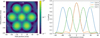 |
Fig. 6 Left: transmission of the PIAAN over the 7 fibers as a function of the object position. Right: 3 cuts through the left map showing the loss of transmission if the companion is not centered, and in particular the blind zones between fibers with transmission dropping to zero (cut B and C). |
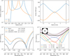 |
Fig. 7 Design and performance of a real PIAAN optics. Top: curvature radius and sag of both aspheres for a CaF2 rod design. Bottom, left: star coupling comparing the geometrical model to physical ones. Bottom, right: star coupling in the presence of VLT spiders. Each color curve represents a different lenslet position angle relative to the displayed pupil on the left corner. θ=0° represents the field position (+37, 0) mas in Fig. 6. Average over all orientations and fibers is shown in gray. |
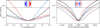 |
Fig. 8 Sensitivity of null to tip (left) and coma (right) for six fibers. Blue and red for fibers 1 and 4, placed in the direction of the aberration. Brown represents fibers 2 and 6 (which overlap due to symmetry), and purple represents fibers 3 and 5 (also overlapping). Black represents the average of the six fibers for all orientations of the aberration. The tolerance limit is shown with the dashed black line. |
Summary of PIAAN tolerances.
2.5.3 Manufacturing errors
To assess feasibility, we also included manufacturing and alignment errors in the model, either in the PIAA optics, in the IFU or upstream in the front-end. Table 2 presents the major tolerances we obtained from the analysis.
We did not perform a study on PIAA sag errors, since they can be compensated with a DM as we present in Sect. 3. The DM correction is only partial, since it can only be conjugated with one of the two PIAA surfaces, but the impact is well within the tolerances. Given current manufacturing capabilities, errors at frequencies beyond the DM correction are so small that they have a marginal impact, mostly on the Strehl/transmission level.
The tabulated values were obtained considering each term independently. To assess the effective performance of a complete system, we also performed a series of Monte Carlo simulations. The values considered are presented in the “MCMC” column of Table 2. Note that we ignored some parameters because we have means to keep them under control during manufacturing or alignment. This includes (1) the PIAA thickness for a rod design, which can be measured prior to making the aspheres, allowing the sag to be adapted; (2) teRMS related to pupil chromatism or pupil size, for which a mask can redefine the pupil at the PIAA level and “hide” the defects. As explained before, we do not consider PIAAN sag errors, so the system considered in this analysis is free of wavefront errors from optics. Results are presented in Fig. 9 in the form of a probability density function for each wavelength. With the tolerances considered, we have an excellent probability of obtaining a PIAAN that delivers ⟨ρ⊙⟩ ∼ 2 · 10−5 the lab. We also investigated the performance when in considering a perfect IFU (Fig. 9, right), and we observed that the quality will increase drastically and very likely reach the design value (ignoring PIAA sag errors). Combined with proper wavefront control, such a PIAAN would probably reach the foreseen contrast levels.
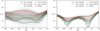 |
Fig. 9 Probability distribution of the PIAAN performance considering manufacturing tolerances. There is no optical aberration in this system, not even on PIAA optics. The gray area is the probability density function for each wavelength. The curves then represent the 10, 25, 50, 75, and 90 percentile of the realizations for each wavelength. They do not represent a likelihood to obtain an actual contrast curve. Left: all tolerances included as presented in Table 2. Right: result when a perfect IFU is considered. |
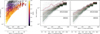 |
Fig. 10 ρ⊙ as a function of the XAO residual error, integrated over three cycles in the pupil diameter. Left: results from different simulations represented by points color coded by Strehl at λ=750 nm. Middle: PSD of all data binned by WFE, shown as a gray map. Green to red curves represent the 10, 25, 50, 75, and 90 percentile of best cases. Right: same as middle, filtered for Strehl≥70%. |
2.5.4 XAO residuals
The XAO residuals are included in the dynamic term of our error budget. Although sensitivity to tip-tilt and coma (or even eigen modes; Sect. 3) give a good idea of the tolerance of PIAAN, we need a more general tolerance specification on wavefront error (WFE) to design the XAO system, which must deal with all possible spatial frequencies. Given the non-linear behavior of ρ⊙ around the design position and the Kolmogorov statistics of atmospheric turbulence, such a tolerance is not straightforward to extract, so we use a statistical approach. We use the analytical model of OOMAO (Conan & Correia 2014) to run several hundreds of XAO simulations for a VLT telescope. We varied the parameters of the XAO like the deformable mirror actuator count (Nact = 40−60) and the loop speed ( f = 1 4kHz), and the seeing conditions (θ = 0.4−1.5′′, vwind = 10 m/s) to vary the loop performance and get a broad range of Strehl and low-order residuals. Given the small working angle, we only consider a pyramid WFS for its sensitivity.
From each simulation, we generated a set of statistically independent residual phase screens, for which we compute the WFE integrated over three cycles in the pupil diameter (which corresponds to the external diameter of our spaxels). This corresponds to about 30 Karhunen-Loeve modes on a DM. The screens are then injected in the PIAAN physical model to compute ρ⊙(WFE(f ≤ 3 cycles)).
All simulation points are presented in Fig. 10 (left), color coded by Strehl ratio. We observe that Strehl (i.e., WFE over all frequencies) correlates moderately well with low-order WFE, illustrating the difficulty of establishing a simple, yet robust, tolerance. For the requirements of RISTRETTO, a Strehl ratio of at least 60% at λ = 750 nm is required to keep ρ⊙ ≤ 7 10−5. This sets a lower limit to the deformable actuator count to· Nact ≥ 30 for a seeing of 0.75′′. A minimum loop speed of 2 kHz also appears to be necessary with a single integrator controller.
In the middle plot, we aggregated the data in the form of probability density functions of ρ⊙ binned by low-order WFE. The five curves present the 10, 25, 50, 75, and 90 percentile of the best performance. The right plot is a filtered version, only including simulations of XAO systems and seeing reaching Strehl ≥ 70% at 750 nm. This filters mainly simulations with the worst contrasts, so that the median performance does not vary significantly. The analysis could also be refined considering a real seeing statistics, or even a real set of observations. The difference between the two distributions, however, suggests we can define a generic requirement based on this statistics. It shows that our dynamic specification is reached for WFE( f ≤ 3 cycles) ≤ λ/100−λ/75, or 8–10 nm RMS at 750 nm.
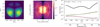 |
Fig. 11 Example of the polarization analysis for the crossed term Exy at the output of a Nasmyth fold mirror. Left: resulting amplitude after the PIAA Middle: PSF. Right: Stellar coupling. The contribution of the two cross polarizations to the PIAAN performance over the six fibers are in color; there is some overlapping due to symmetry. The two lowest curves correspond to the fibers in the horizontal direction. |
2.6 Polarization aberrations
Polarization dependent wavefront aberrations are due to asymmetries in mirror reflections and are a known limitation for high contrast instruments (Breckinridge et al. 2015). Variations in the angle of incidence across reflective surfaces (concave or convex mirror, fold mirror in converging beam) lead to spatially dependent changes in electric field amplitude (diattenuation) and phase (retardance), locally altering the state of polarization (SOP). This leads to multiple independent point spread functions at the focal plane, one for each combination of parallel and cross-polarization teRMS. The undesired crossed polarizations also have a typical size of 2 λ/D due to the asymmetry in the reflection, which could be particularly harmful for such a narrow working angle. In the case of unpolarized light, such an effect cannot be corrected.
We use Zemax Optics Studio software to propagate linear SOP via ray tracing in a model of the VLT, including the M3 fold mirror toward the Nasmyth platform. It also includes a K-mirror derotator placed after the VLT focus in the f/15 diverging beam: it is made of 2 mirrors with angle of incidence (AOI) of 60°, and 1 mirror with AOI=30°. For a given 2D input linear polarization Ex or Ey, Zemax computes the complex electric field in the exit pupil (Exx, Exy, Eyx, Eyy). Those electric fields are injected into our PIAAN model as input pupil illumination (instead of a uniform one) to assess its behavior over the 4 exit SOP. For each input state, the total coupling is the sum of both exit teRMS (e.g., ρx = ρxx + ρxy). Fig. 11 (left and middle) presents the resulting propagation for Exy alone through the PIAA optics. As expected, the core spreads slightly in the external lenslets, although it is well contained thanks to the apodization. The contrast of this PSF is much lower than that of a uniform pupil (the rings have a relative intensity of ∼10−2), but it still contains many destructive rings throughout the lenslet. The total energy in the cross polarizations being also ≤10−3 from the input, the contribution of the cross polarization is negligible, generally well below 10−7, i.e. 10–100 times below the design value (Fig. 11, right).
The K-mirror rotator may also constitute an important source of polarization aberrations. Considering a K-mirror with a 0 or 90° orientation with respect to the M3, the effect between Exx and Eyy is a differential tilt with respect to the unpolarized beam, with an amplitude of less than 10 nm PV (≤ λ/D/60 in the visible, or 0.25 mas PSF offset), which is negligible in our case. In the end, the K-mirror also has a negligible impact on coupling and contrast. Polarization aberrations are therefore negligible for the considered contrast levels with 2 λ/D size lenslet.
3 Wavefront control with the PIAAN
3.1 Objective
Considering the tight tolerances, wavefront control is fundamental to make the PIAAN operational. Not only is the wavefront error requirement extremely stringent, but any defect in the PIAA optics or IFU manufacturing will shift the optimum working point from the natural design solution that assumes a flat wavefront or even prevent it to work at the desired level. A dedicated wavefront sensor near the IFU does not appear as a viable solution at such low tolerance to low-order WFE, so we investigate how to perform wavefront sensing and control with the PIAAN itself. Our goal here is to correct for static errors (PIAAN defect and static WFE) to reach ⟨ρ⊙⟩ ≤ 7 · 10−5.
3.2 Principle
Our strategy is inspired by Give’on et al. (2007) and Por & Haffert (2020), and is also similar to the idea of Implicit Electric Field Conjugation applied to SMFs (Liberman et al. 2024), extended to a fiber bundle here. We measure the coupling variations, δρi, of each fiber to small input phase disturbance, δx. In our case, we pushed the individual actuators of a deformable mirror, with a typical amplitude of a couple of nanometers. Testing all actuators, we built an interaction matrix, M:
 (4)
(4)
The eigen mode decomposition of M leads to a series of seven modes (Fig. 12, top), which can be used to optimize coupling on each fiber more or less independently (Fig. 13). If we include the central fiber in the analysis, the first mode corresponds to the WFE that maximizes on-axis coupling. The other six modes allow for the control and optimization of contrast over the six external fibers. For a perfect PIAAN, only three of those modes have a real influence (three high eigen values) due to the symmetry: one cannot change the contrast on one fiber without acting on the opposite one. As long as we deal with pupil phase errors, such modes allow the contrast to be corrected to its design value. Those modes can actually be decomposed as a sum of Fourier modes with frequency of about two cycles, and orientations of 0°, 60°, and 120°, corresponding to the lenslets position. With defects, an asymmetry appears and this behavior becomes clearer: Fourier modes shift slightly in frequency and phase over the pupil (Fig. 12, bottom) and act more and more on individual fibers, since their variations tend to decorrelate. By construction, the eigen modes are the least tolerant modes, and we notice that our specification of ρ⊙ ≤ 7 · 10−5 is reached with less than 1.5 nm RMS (λ/500) variation (Fig. 13). This result demonstrates the necessity of using the PIAAN signal for performing fine wavefront control and optimization.
Since we measure a coupled intensity and not an electric field amplitude, we cannot measure a totally linear response. The analysis is therefore only valid locally near the calibration point. If the probe is too large, we actually risk to probe through a local maximum or minimum of coupling, invalidating the linearity hypothesis of the method, and estimating modes inaccurately. So, the calibration step size must be small enough, of the order of a couple of nanometers, and the procedure iterative to get modes as accurate as possible. Performing the probe with a DM upstream from the PIAA, we also end up with a set of calibrated commands, accounting for its non uniform (or even time varying) response through that optics. Since the method is by nature sensitive to only 7 low-order modes, it remains difficult to solely rely on it for a global wavefront error compensation. The method is in particular flawed if the IFU is not perfectly centered on the PIAA optical axis: our PIAA design transfoRMS about 5% of the entrance tilt into a coma-like aberration, so that applying a coma upstream can compensate for a big part of the off-axis aberration. The method therefore applies once the system is already well aligned. Since our coma tolerance amounts to ±0.005 wave, a good alignment would represent a tilt error of ±0.1 λ/D , which is relatively easy to achieve thanks to the quickly growing coma-like aberration.
We also note that there are different ways to build and use M:
Firstly, a polychromatic analysis can be performed by stacking more measurements in
 for a given probe. More modes could also be reconstructed in that way; every test wavelength will be sensitive to slightly different spatial frequencies, bringing some diversity to the analysis, and allowing the full benefit from a higher density DM to be taken. Ideally, the eigen values should present three dominant teRMS, indicating that the contrast can be optimized by pairs of fibers, and independently of wavelength.
The performance of the PIAAN assumes a perfectly rotational symmetric aperture. Any deviations, such as telescope spiders, masked dead actuators, and IFU defects, change this figure so that the method can also be used to find the optimal working point and balance performance between the six fibers. The very limited size of such deviations could nevertheless require higher spatial frequencies than delivered by a low-order DM.
Considering the IFU must be rotated to fill holes in its azimuthal transmission (Fig. 6), we can either estimate modes for different orientation, or stack the response at different orientations, to obtain circularized modes, independent from the IFU orientation.
Finally, we can perform the analysis on a subset of fibers. If the companion position is known, we can choose the best fiber to use and determine the one mode of interest. The complete system can be optimized for it, including the XAO, with a dedicated controller optimized to reduce, for instance, the impact of lag and vibrations.
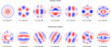 |
Fig. 12 Top: the seven eigen modes obtained after calibration for a perfect PIAAN. Bottom: the eigen modes in presence of defects. |
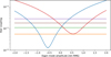 |
Fig. 13 Example of coupling variation over the six external fibers for a scan of a given eigen mode to which two fibers are sensitive. |
3.3 Procedure
We tested the method in the simulation with an 11 × 11 DM, which can in principle correct spatial frequencies beyond the field of view of the PIAAN. We also considered for these simulations that the IFU is perfectly aligned to the PIAA optical axis.
As a first sanity check, we applied a known aberration in the DM plane (either defined by hand or following an f−2 power law), and run an eye-doctor technique with 50 Zernike modes: the injected aberration is fully recovered after 2 iterations by optimizing coupling (i.e., Strehl) on the central fiber, with a couple of nanometers of reconstruction error. We then use the proposed calibration method using the first eigen mode: after 1 calibration of the DM and 1 scan of the eigen mode, the phase is recovered with a very minor difference with the Zernike modes.
We then added complexity with manufacturing and alignment errors on the PIAA and IFU, considering the values already presented in Table 2 for the Monte-Carlo simulations. We also added 30 nm RMS of sag error on both PIAA surfaces, which we try to compensate for. We proceed in two steps:
Step #1 - Wavefront correction - We calibrated M a first time and optimize coupling on the central fiber with the first eigen mode, as described before. This already recovers a big part of the performance, in particular the PIAA errors (Fig. 14, middle). We skip this step if we consider the IFU alone (Fig. 14, top).
Step #2 - Contrast optimization - Due to defects in the IFU and Fresnel propagation in PIAA (Talbot effects), ρ⊙ is not yet optimal and it presents strong inhomogeneities with wavelength and between fibers. We recalibrate M with only the 6 external fibers to optimize ρ⊙. For each eigen mode, we perform small scans around the calibration point (similar to a standard eye-doctor procedure), with amplitude between 1 and 5 nm RMS. Since we do not know the optimal value of ρ⊙ we want and can reach, this scan is necessary, we cannot simply inverse M to reach a given contrast. We are not interested in obtaining extremely deep nulls at a particular wavelength: our goal is instead to obtain a balanced system, so that SNR is also balanced between fibers and at all wavelengths. So, we minimize the dispersion of contrast over the 6 external fibers for each scan, instead of optimizing contrast for one particular fiber (the procedure actually does not converge easily if we proceed that way). For systems within our tolerances, 2–3 calibrations over the 6 modes is enough to converge without an apparent ambiguity. Once close from an optimal solution, optimizing two opposite fibers at a time also appears to be more effective. If during an iteration, the working point moved too much, the fibers get naturally less independent for a given eigen mode and an intermediate calibration is performed.
We demonstrate this procedure with PIAA or IFU errors alone, and finally the complete PIAAN (Fig. 14), with a common set of errors to evaluate the impact of each component. We perform a monochromatic optimization at 730 nm. With sag errors, ρ⊙ starts at ∼10−4, with variations by a factor 10 between wavelengths and fibers. The DM is particularly effective for compensating the PIAA errors and balancing contrast. It is a bit less effective with the IFU, the far-field of the SMF being conjugated to the focal plane. Introducing only fiber core misalignment leads to better results, with almost complete recovery of the design performance. This is more difficult with far-field alignment errors. We notice the benefit of the PIAA apodization, which allows contrast optimization at no cost on transmission with a wavefront offset below 2 nm RMS.
All errors considered, we seem to reach a limit at about 1 · 10−5 (also observed with different sets of errors). This is probably due to off-pupil errors (Talbot effects and IFU errors) that we attempt to correct with a single pupil DM. Without too much surprise, doubling the actuator density does not change much the eigen modes nor improve the end results.
The contrasts achieved are about a factor 7 better than our requirements, so that performance should ultimately be limited by XAO performance (see Sect. 2.5.4 and Fig. 10), so we do not study the benefit of a second DM in a focal plane. This leaves us sensitive to Talbot effects and limits our capability to fully correct aberrations and reaching the design value. We performed a couple of simulations including several 2f-2f optical relays, made of commercial 1′′ optics with wavefront error ∼λ/4 P-V, used at f/50 with a beam size of 4 mm. The impact after the optimization procedure was negligible and do not require a focal plane DM. It could still be useful to correct IFU manufacturing errors, but this was not explored as we believe we can make IFUs of appropriate quality. It is worth noting that this method could be applied to any single-mode fiber coronagraphic IFU.
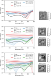 |
Fig. 14 Result of wavefront control with IFU error only (top), PIAA errors only (middle), and the full PIAAN (bottom). Red, blue, and green curves correspond respectively to the start point (DM flat), the result after WFE optimization, and the result after contrast optimization. The filled area corresponds to the envelope covered by the six fibers and the solid line to their average. The resulting DM shaped applied after each step is shown on the right of the plots. M is calibrated at 730 nm. |
3.4 Non common path aberrations in operations
In practice, we would want to find the working point of the PIAAN during integration or daily calibrations. The working point, limited by the PIAAN alignment and defects, should be stable in time. Optical aberrations are more prone to evolve over a timescale of 1 hour and with amplitudes significant for small inner angle coronagraphs (Vigan, A. et al. 2022). During the night, non common path aberrations could be calibrated on an internal light source: with a camera working at several 100 Hz (or even photodiodes much faster than any DM settling time), and fast flip mirrors and shutter. Such a calibration could be performed in a couple of seconds during an hour-long exposure.
4 Prototyping and test results
4.1 Integral field unit
The IFU unit consists in a bundle of seven standard step-index SMFs, packed in an hexagonal array. A micro-lens array is then 3D-printed on top of the bundle. We thoroughly characterized their performance to eventually adapt the microlens design, as well as to estimate the readiness level of the novel 2-photon polymerization 3D technique for astronomical use.
4.1.1 The single-mode fibers
We used off-the-shelf Thorlabs SM630HP SMFs with a core diameter of 3.5µm and NA=0.13. They were thoroughly characterized, in particular regarding the NA which must be known to better than 5% to optimize the MLA design. We directly image their far-field on a CCD, without optics. We acquire images at different CCD-to-fiber distances, which allows the extraction of the exact distance for each step and measurement of the angular scale of the setup. A theoretical LP01 mode is then fitted to the data. We measured several samples coming from Thor-labs (bare or connectorized) or a sample provided by SQS/AMS with their bundle. We estimated NA(1/e2) = 0.083 (±3%) which corresponds to geometrical NA=0.120 instead of the data sheet 0.130 (Fig. 15). This leads to a single-mode cut-off wavelength of 550 nm.
One of the fiber characterized here is kept as a reference for future comparative tests, with the bundle and IFU in particular.
4.1.2 Bundle arrays
Fiber bundles prototypes were produced by AMS/SQS with a pitch of 125 µm (Fig. 16, A), after removing the fiber coating. For these prototypes, we use an “octopus” configuration, with seven FC/PC fibers as output of the hexagonal bundle. For the final bundle, the seven fibers will be grouped in a linear slit at the output.
The two bundles are of excellent quality, with a core-to-core pitch of 125 ± 0.7 µm as estimated from a Gaussian fit to the modes. Far-field co-alignment (i.e., mechanical parallelism of fibers), as well as perpendicularity to the mechanical surface, is also well below 0.3° for all fibers (see Table 3).
4.1.3 Micro-lens arrays
The micro-lens array (MLA) is made by Keystone Photonics (formerly Vanguard) using the two-photon polymerization 3D printing technique. The technology allows for maximum flexibility and accuracy in order to create lenses that are optimized for the bundle. The technology promises the alignment of every fiber core to their respective lenslets optical axis with an error of ± 100 nm, well in the PIAAN specifications. A first prototype with a pitch of 250 µm was tested and showed encouraging results (Kühn et al. 2022). The large pitch led to a very complex fabrication process, requiring high volume to print, multiple printing passes, realignment of the machine, etc. A second prototype with a minimal pitch of 125 µm, matching the fiber bundle pitch, was produced with a height of 0.7726 mm. As seen in Fig. 16 (B to D), the lenslets present some structures on the edge, and five printing layers are visible. Despite the straight pillar design, leakage and coupling from one fiber to the other was not observed at the level we are interested. The physical distance between the cores certainly helps in this. For one prototype, one MLA surface was measured by Keystone with an interferometer: the sag is extremely accurate and presents a 10 nm annular structure on its surface, due to the printing technique. Injecting those data in a model of the MLA shows it has a negligible impact on performance, with only a few percent of light lost.
On all prototypes, we also observed a systematic global tilt of ∼1° of the fiber bundle far-field when back-illuminated onto the MLA. The reason is not clear since we measured that the far-field is perfectly perpendicular to the bundle surface (see the previous section), and no such angle is observed between the bundle surface and the MLA. This surface is also used by Keystone to align the bundle onto their machine. In theory, this should have a limited impact on contrast.
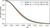 |
Fig. 15 Thorlabs SM630HP NA characterization for different fibers (color lines). SMF models in dashed and dotted black lines. |
4.1.4 IFU performance
To characterize the IFU, we used a simple bench, the same presented in Restori et al. (2024). It is made of two doublet lenses working at f/100 to get a proper plate scale of 2 λ/D =125 µm at the MLA level. The IFU is placed at the bench focus on a 5-axis motorized stage to optimize coupling into fibers. We back-illuminate the IFU to align it angularly to the pupil, and laterally to the input fiber. After this preliminary alignment, there is no ambiguity in optimizing the 5-axis by injecting light from the bench source to the IFU.
The IFU was tested alone with a clear pupil mask, i.e., without central obstruction or spiders. We estimated its transmission in a fixed configuration similar to the sky one. The coupling was first optimized on one particular fiber in XYZθxθy. The Zθxθy positions were then fixed, and the IFU was moved laterally in XY at the bench focus to optimize coupling over the 6 other fibers. We tried the initial optimization on different fibers: no fiber showed significantly higher transmission, and global transmission of the IFU was more or less equivalent regardless of the fiber used for optimization.
In this configuration, the maximum theoretical coupling amounts to  at λ = 633 nm. However, the measurements lead to maximum couplings between 36 and 57% (Table 3). This is a very encouraging result considering how recent the technology is and the difficulty to print such large lenses. However, this is not sufficient to take full advantage of the PIAAN transmission. This results in integration times that increase by 40–100%, depending on the noise regime of the spectrograph (Eq. (1)).
Several tests were performed to understand these measurements and identify the origin of the loss. We considered MLA defects such as polymer absorption due to premature aging due to UV irradiation, wrong lens parameters, and volume grating effects. In parallel, we developed a physical model of the IFU that includes all the knowledge we have of the MLA, including measurements provided by Keystone (e.g., polymer refractive index, lenslet SAG measurements, lenslet height measurements) and our own measurements (e.g., SMF bundle properties, IFU far-field misalignment) for a complete analysis. The different bench tests that we performed were also simulated for comparison, and some fundamental parameters were adjusted to observe their impact. We were nevertheless unable to reproduce the measured transmission considering a reasonable range of values. Despite those disappointing coupling values, we could still obtain very high contrasts, as presented in Sect. 4.4.
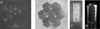 |
Fig. 16 IFU prototype with 125µ lenslet size. (A) Bundle front face. (B) Same view as (A) after the MLA has been printed on it. (C) Side view of the MLA, with illumination from the back, showing some of the printing structure. The lenslet height is 0.7726 mm. D) Three-quarter view showing the seven lenslets. A laser source is injected from the fiber to the lenslet for one of them. Diffusion in the lens material shows the beam. |
Fiber bundle and IFU measured performance.
4.2 PIAA optics
Two PIAA optics were produced by Nutek, with the rod CaF2 design presented in Sect. 2, with a pupil of 4 mm in diameter and a glass thickness of 20 mm (Fig. 17). The centering of both aspheres must be kept below 30 µm, which was well within Nutek capabilities. The thickness of the CaF2 blank was measured prior to turning the optics, allowing one to adjust the sag of both surfaces. The rather small sag and choice of a rod design led to an excellent optical quality, with transmitted WFE ≤ 30 nm RMS for both prototypes (Fig. 17). The PSF obtained on a bench working at f/100 confiRMS the very high optical quality even at visible wavelength (λ=633 nm). It looks slightly more apodized than expected, and not having access to a machine able to measure both sag, it is difficult to estimate its origin. This could have a negative impact on the contrast performance by changing the balance between the rings.
4.3 Experimental setup
4.3.1 Design
We built a bench to characterize the PIAAN (performance, stability) and to test the wavefront control strategy with a DM. The goal of this bench being a polychromatic characterization of the PIAAN, the bench is reflective. A refractive solution with off-the-shelf components f/100 beams was also studied. Chromaticity of this solution was theoretically well within our WFE specification over 30% bandwidth, but it was unclear if produced optics can match it, which would have left us with strong doubts on PIAAN performance if they were not reaching expectations.
The bench is built exclusively from off-the-shelf components. The main path of the bench (Fig. 18) consists of three replicated Off-Axis Parabola (OAP1, OAP2, OAP3) with f=279 mm (Edmund Optics EO90-978 / Shimadzu 275-07-4040) working at f/70, and a fourth f=254 mm 30° OAP (Thorlabs MPD2103-P01; OAP4) working at the optimal f-number of 63.5 for an IFU with 125 µm lenslets. A Boston Micromachines Multi-3.5 DM (12x12 actuators) is placed between OAP1 and OAP2 to control wavefront in the bench. A chromium pupil mask and the PIAA optics are conjugated to the DM in a pupil plane between OAP3 and OAP4. The chromium mask defines the pupil and is placed about 1 cm before the PIAA, which is within our tolerance for a 4 mm pupil size. The PIAA is mounted inside a four-axis gimbal mount (Standa 5GTM1). The IFU is placed on a 5-axis motorized stage: three-axis translation stage (Thorlabs MTS25) to align the IFU to the PIAA optical axis, and a 2-axis motorized Gimbal mount (Zaber OMG) to align the IFU far-field to the PIAA pupil.
Post-PIAA focal and pupil imaging are provided thanks to a pickup beam splitter, followed by two cameras, to image the post-PIAA focal plane and pupil. The beam splitter presents a small wedge dispersing the PSF at the IFU level, so a second plate with an equivalent wedge is placed after to compensate it. We also placed a retro-reflector near BS1 (not shown Fig. 18) for alignment of the IFU to the VLT pupil and source.
To perform polychromatic measurements, a simple fiber-fed prism-based spectrometer was built (Fig. 18, top). The IFU bundle is connected to another bundle, made of 7 multimode fibers with 50µm core, rearranged in a slit. The choice of multimode fibers was made to limit chromatic coupling effect at the connector level, that could bias the characterization. The spectrograph resolution is limited by the fiber size to 100. The dispersed fiber signal naturally presents a high modal noise, but since we are interested only by information at a resolution of a few 10, it averages well and we did not add a mechanical scrambling device. Due to the limited dynamic of the spectrograph camera, the central fiber is attenuated by putting both the central IFU fiber and central slit fiber ∼20 mm apart, leading to an achromatic and very stable attenuation factor of 400. Measurement over a dark area of the sensor shows that contrast is limited to 10−7 in a single exposure. The wavelength scale is calibrated by using 3 laser sources at λ=638, 730 and 850 nm.
The full bench and spectrograph are placed under an enclosure to eliminate turbulence and stray light.
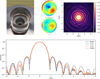 |
Fig. 17 PIAA prototype. Top, left: picture of one PIAA optics before coating. Top, middle: WFE of both prototypes as measured by Nutek. Top, right: PIAA PSF in log scale at λ=633 nm. Bottom: cut views and radially integrated profile, compared to the theoretical PIAA PSF in black. |
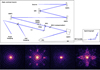 |
Fig. 18 Top: optics Studio design of the RISTRETTO high contrast bench and spectrograph. Bottom: PSFs at the IFU level at λ = 633 nm. The two on the left are obtained with a VLT pupil, with a flat mirror in place of the DM for preliminary alignment, and with DM optimized in a best flat position. The two on the right show the same, after aligning the PIAAN, also with flat mirror and with best flat DM. |
4.3.2 Alignment and characterizations
Optical alignment of the bench based on the Optics Studio and a Solidworks modeling proved very reliable. The high f-number is very forgiving, leading to tolerance on the OAPs alignment of the order of ± 2 mm and ± 1° regarding WFE. The final f-number is accurate to 0.5% after measurement of the PSF at focus.
The pupil of the system is defined by the chromium mask positioned just in front of the PIAA. Different pupils are available: a 4 mm pupil without central obstruction and a 4 mm VLT pupil without the spiders, and variations of these two pupils with a slightly oversized or undersized primary and secondary. This resulted in aperture diameter varying from 3.6 to 4.4 mm in 0.08 mm steps, and in secondary obstructions with a diameter varying from 0.64 to 0.78 mm in 0.03 mm steps, step size being related to the tolerance on the pupil magnification. The mask was patterned using photolithography with smallest details of 1 µm. Note that the PIAA optics has been designed to reduce the VLT obstruction of 16%. However, it appears that the secondary obstruction in the mask has no impact on the performance, as long as it is smaller than the one considered for the PIAA design. We therefore used the one without obstruction to remove a degree of freedom.
The deformable mirror was characterized using an interferometer with a 5 mm beam. The response matrix of the DM was computed from this calibration, which was then used to compute a best flat command set, leading to a final surface error of 18 nm RMS, dominated by the DM actuator structure at 12 cycles.
The bench was first aligned with a flat mirror in place of the DM, and shows an excellent optical quality (Fig. 18, bottom) without and with the PIAA optics. The optical quality of this reflective bench is lower than our original refractive IFU test bench, designed at f/100 (Restori et al. 2024), and also used to obtain the PIAA PSF of Fig. 17. The quality is actually limited by the last diamond turned OAP4, which presents a roughness of 10 nm RMS. At the IFU focus, we do not observe ghosts from the usual grating structure resulting from the diamond turned manufacturing. The PSF measured at the IFU focus is nevertheless clearly of lower optical quality than the one observed on the imaging arm, where only lenses are used: we observe twice more diffraction rings on the latter and integrated PSF profiles defer at ∼10−6 contrast level.
The DM was aligned visually to the pupil mask by pulling four actuators in a square shape around the secondary obstruction. The pupil camera was then used to center the resulting structure to the pupil mask. Since the pupil is smaller than the DM active surface and the wavefront control procedure calibrate the DM influence on coupling, an accurate centering is not required.
To maximize Strehl ratio, we used an eye-doctor technique, using a Zernike basis or the DM eigen basis. Both methods showed similar results. We obtained best results when normalizing the PSF to the energy contained within the correction area of the DM. While the PIAA PSF is improved, the diffraction rings still show some roughness, and in the case of the second and third rings a slight asymmetry. We can observe the strong off-axis aberration of the PIAA to the satellite spots at 5 λ/D , generated by the DM structure (as well as much fainter at 7.5 λ/D ). The DM best flat measurement was injected into the PIAAN model, degrading the null to ⟨ρ⊙⟩ ∼ 2 10−5. This can be considered as the performance limit of this bench since those structures cannot be corrected by the DM itself.
Those spots cannot be removed with a spatial filter at an intermediate focus, since it would filter the pupil for which the PIAA has been designed. A DM with a higher number of actuators might be required to push the satellites further in a future implementation.
The final alignment consisted in putting the PIAAN. We started with the IFU, aligning it in XYZθxθy until the coupling is maximized on the central fiber. The central fiber was back-illuminated to see it on the focal and pupil plane cameras thanks to the retro-reflector, together with the VLT pupil and source coming forward. We performed a preliminary alignment that achieved a couple of percent coupling into the central fiber. We then optimized the coupling using a powermeter and the 5-axis motorized stage with an automated, recursive procedure until we reach about 50% coupling on the central fiber. Following this step, the IFU is aligned to the bench optical axis. We final inserted the PIAA optics and aligned it laterally to the pupil and angularly to the bench optical axis. Because of its non-linear transformation of the electric field, PIAA presents very peculiar figures if slightly misaligned (Fig. 19):
Field alignment - The PSF first ring gets very quickly distorted if the PIAA angular alignment is wrong. The distortion is visually obvious with 0.2 λ/D error, so we estimate that we can achieve a visual field alignment error below 0.1 λ/D .
Pupil alignment - The central obscuration on the PIAA exit pupil becomes quickly asymmetric with a slight offset error of just 1% of the pupil diameter. We estimate that our pupil alignment error is below 0.5% of the pupil diameter.
In practice, thanks to the monolithic nature of our optics, the alignment was performed visually in a couple of minutes.
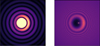 |
Fig. 19 Illustration of PIAA misalignment errors on the focal and pupil plane cameras. Left: PSF for 0.2 λ/D tilt error. Right: central 1 mm of the exit pupil for 1% pupil diameter error. |
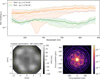 |
Fig. 20 Top: result of the contrast optimization of PIAAN. The starting point is in orange, after Strehl optimization. The filled area shows the envelope covered by the six spaxels, each shown by a colored curve in the envelope. The end result is displayed in green, also with the curve of the six spaxels and the corresponding envelope in green. Bottom left: working point OPD applied on the DM. The yellow circle represents the 4 mm pupil size of the PIAA. Bottom right: resulting PSF at λ=633 nm. |
4.4 PIAAN performance and wavefront control
We finally put our full prototype and optimization procedure to test. We measured the flux in the spectrograph over the seven fibers sequentially, both on- and off-axis.The on-axis measurement is used to estimate  over the six external fibers, through six on-axis flux measurement
  . By adding a 2 λ/D tilt on the DM to center the PSF on the desired spaxel, we estimate
  for the six fibers, with sixflux measurements
  . The contrast of the six fibers is then estimated as
 (5)
(5)
Since we used a spectrograph, the contrast was estimated for different wavelengths. We estimated ρ⊙ as
 (6)
(6)
with  the PIAAN transmission at 2 λ/D , which was measured in Sect. 4.1.4. However, due to the low measured transmission of the IFU, we would obtain an artificially favorable estimation of ρ⊙, compared to theoretical values. We therefore decided to scale the contrast estimation with the theoretical PIAAN transmission instead, at the measurement wavelength of λ = 633 nm, i.e., ρ⊕(λ = 633 nm) = 0.67 (Fig. 4). For each of the sixexternal fibers, our estimator of ρ⊙ is finally:
 (7)
(7)
We started by calibrating the DM through the PIAAN to compute the eigen modes (step 1 in Sect. 3.3), and correct wavefront with the first mode. This corresponds to an additional Strehl optimization, compensating the WFE between the initial eye-doctor on the focal plane camera and the PIAAN. We could actually observe very little (if any) gain with this step, indicative of a very small amount of differential aberration between the IFU and the imaging camera. We generally obtain relatively good nulls, with ⟨ρ⊙⟩ = 2.7 · 10−4 (Fig. 20, orange curve), averaged over the 6 spaxels and all wavelengths between 620 and 840 nm. This is 5 times higher than expected from the tolerance analysis (Fig. 14, bottom). The dispersion over wavelength and spaxels amounts to 2 · 10−4 RMS.
We then look for the working point (step 2 in Sect. 3.3). After a new calibration, we scan successively each eigen mode and apply the appropriate amplitude to minimize ρ⊙ on each spaxel successively. The procedure is repeated several times with intermediate calibrations, and eventually converges in less than 20 iterations. With our current setup, it takes about 30 min, limited by the frame rate of the spectrograph camera, around 10 Hz. We eventually reduce ⟨ρ⊙⟩ by another factor 10. With the OAP4, we obtained ⟨ρ⊙⟩ = 5.0 · 10−5. For the reasons explained before, we exchanged this OAP for a doublet lens (Thorlabs AC254-250-A), with higher optical quality, and chromatic errors in principle below our requirements. We could then consistently obtain better contrasts, down to ⟨ρ⊙⟩ = 3.5 · 10−5 with a dispersion of ±1 · 10−5 RMS over wavelength and spaxels. We present the latter results in Fig. 20 (green curves). We attribute the lower performance of the OAP to its much higher surface roughness: since it is outside the pupil plane, the speckles created at the IFU focal plane in the 1–3 λ/D area can only be partially compensated by the DM. The demonstrated performance is consistent with expectations, considering the effect of the DM structure and various errors in the system.
The full optimization procedure was repeated 80 times over 72 h to test its robustness, starting from the same DM flat and contrast. The repeatability is excellent with a dispersion of ±1 · 10−5 RMS for each spaxel and wavelength. The start point remains nearly identical from one test to the other.
The optimal pattern on the DM is shown in Fig. 20 (bottom) and is larger than anticipated in Sect. 3, with an optimal wavefront of 20 nm RMS (∼λ/30 −λ/40), leading to a relative transmission degradation of the PIAAN of 2.6%, or ⟨ρ⊕⟩ = 70%. Over the 80 repetitions, the DM shape varies by 1.0nm RMS.
We also tested different pupil masks within 1% of the optimal one. After the optimization, we always obtained ⟨ρ⊙⟩ ≤ 5 10−5.
We finally performed stability tests. First a 72h long stability test has shown that contrast degradation is dominated by tip-tilt drift of the bench: after correction with the DM, the spectra of the 6 external spaxels overlapped perfectly with the initial ones. Note that the correction was applied according to the focal plane camera position, i.e., with a potential differential aberration. We also performed a week long stability test (Fig. 21, left), where only tip-tilt corrections were applied every 1 hour, still according to the focal plane camera. Between day 2 and 5, a +1 K temperature step was applied. The cumulated DM corrections indicate a bench drift of 0.2 λ/D, while average contrast correlates to temperature at a rate of ∆ρ⊙/∆T ∼ 1 10−5K−1. Over the week, we still observe a slow drift of contrast of ∆ρ⊙ ≃ +1 · 10−5 uncorrelated to temperature. A new contrast optimization of PIAAN allows it to recover the initial performance. Therefore, stabilizing the PIAAN environment to 1K should easily keep PIAAN operational for a full night.
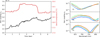 |
Fig. 21 PIAAN stability measurement over a week, with hourly tip-tilt correction. Left: average contrast over the six fibers (black), and bench temperature (red). Right: contrast curves for the three most unstable fibers (#2, #4, and #5). There is a 24h time span between each curve, from blue to red. |
5 Conclusion
We have presented PIAAN, a high transmission (ρ⊕ = 0.72), high contrast (ρ⊙ = 7 · 10−7) and broad band (∆λ = 30%) coronagraphic IFU for HDC, designed for observing companions orbiting at about 2 λ/D from their host star. It is the baseline for RISTRETTO, to characterize Proxima Cen b with the VLT.
After presenting the concept, we performed a complete tolerance analysis to evaluate its manufacturability and identified the limits between the ideal design and the feasible one. PIAAN shows excellent robustness to tip-tilt jitter, a major limitation of XAO systems in the presence of vibrations or wind shake. A wavefront optimization strategy has also been developed to manage defects that are identified (or not) in the tolerance analysis.
Finally, we designed and tested a complete prototype that reached performance in agreement with our expectations from the initial tolerance analysis, i.e., ρ⊙ = 3.5 · 10−5. We also investigated of the use the recently developed 3D printing capability offered by twp-photon polymerization technology to produce a compact, stable, and fully integrated IFU. This technology demonstrates a very encouraging maturity level, especially considering that our design requires a high volume to be printed, at the current limit of the technology. We will continue to explore the capabilities of this technology in order to reach the maximum transmission allowed by PIAAN.A bulk solution might also be considered otherwise, as it should allow for a full control over the different degrees of freedom of the IFU to reach the theoretical maximum coupling.
The development of coronagraphs such as PIAAN that provide high throughput and very small IWA is fundamental to fully exploit the spatial resolution and collecting area of large telescopes, particularly the future generation of ELTs, for which observing time will be very costly. The performance of PIAAN and its high tolerance allow in addition constraints on the XAO system to be relaxed for such large aperture. The impact of the apparent diameter of the nearest stars with bigger telescopes is also limited.
Acknowledgements
We thank the anonymous referee whose thorough comments improved the quality of this paper. The authors would like to thank Dr. Olivier Guyon for his interest in this work and the fruitful discussions. This work has been carried out within the framework of the National Center of Competence in Research PlanetS supported by the Swiss National Science Foundation under grants 51NF40_182901 and 51NF40_205606. The RISTRETTO project was partially funded through SNSF FLARE programme for large infrastructures under grants 20FL21_173604 and 20FL20_186177. The authors acknowledge the financial support of the SNSF. C.M. acknowledges the support from the Swiss National Science Foundation under grant 200021_204847 “PlanetsInTime”.
References
- Beuzit, J. L., Vigan, A., Mouillet, D., et al. 2019, A&A, 631, A155 [NASA ADS] [CrossRef] [EDP Sciences] [Google Scholar]
- Blind, N., Shinde, M., Dinis, I., et al. 2024, SPIE, 13097, 130976U [Google Scholar]
- Breckinridge, J. B., Lam, W. S. T., & Chipman, R. A. 2015, PASP, 127, 445 [CrossRef] [Google Scholar]
- Conan, R., & Correia, C. 2014, SPIE, 9148, 91486C [Google Scholar]
- Denis, A., Vigan, A., Costes, J., et al. 2025, A&A, 696, A6 [NASA ADS] [CrossRef] [EDP Sciences] [Google Scholar]
- Echeverri, D., Ruane, G., Jovanovic, N., et al. 2019a, SPIE, 33, 1117 [Google Scholar]
- Echeverri, D., Ruane, G., Jovanovic, N., Mawet, D., & Levraud, N. 2019b, Opt. Lett., 44, 2204 [Google Scholar]
- Echeverri, D., Xuan, J., Jovanovic, N., et al. 2023, J. Astron. Telesc. Instrum. Syst., 9, 035002 [Google Scholar]
- Give’on, A., Kern, B., Shaklan, S., Moody, D. C., & Pueyo, L. 2007, SPIE, 6691, 66910A [Google Scholar]
- Guyon, O., Pluzhnik, E. A., Galicher, R., et al. 2005, ApJ, 622, 744 [NASA ADS] [CrossRef] [Google Scholar]
- Haffert, S., Por, E. H., Keller, C. U., et al. 2020, A&A, 635, A56 [NASA ADS] [CrossRef] [EDP Sciences] [Google Scholar]
- Jovanovic, N., Martinache, F., Guyon, O., et al. 2015, PASP, 127, 890 [NASA ADS] [CrossRef] [Google Scholar]
- Jovanovic, N., Schwab, C., Guyon, O., et al. 2017, A&A, 604, A122 [NASA ADS] [CrossRef] [EDP Sciences] [Google Scholar]
- Kühn, J. G., Blind, N., Chazelas, B., Hocini, E., & Lovis, C. 2022, SPIE, 12188, 121881T [Google Scholar]
- Liberman, J., Llop-Sayson, J., Bertrou-Cantou, A., et al. 2024, J. Astron. Telesc. Instrum. Syst., 10, 029002 [Google Scholar]
- Lovis, C., Snellen, I., Mouillet, D., et al. 2017, A&A, 599, A16 [NASA ADS] [CrossRef] [EDP Sciences] [Google Scholar]
- Lovis, C., Blind, N., Chazelas, B., et al. 2024, SPIE, 13096, 130961I [Google Scholar]
- Lozi, J., Martinache, F., & Guyon, O. 2009, PASP, 121, 1232 [NASA ADS] [CrossRef] [Google Scholar]
- Macintosh, B., Graham, J. R., Ingraham, P., et al. 2014, Proc. Natl. Acad. Sci., 111, 12661 [NASA ADS] [CrossRef] [Google Scholar]
- Males, J. R., Close, L. M., Haffert, S. Y., et al. 2024, SPIE, 13097, 47 [Google Scholar]
- Marcuse, D. 1973, Bell Syst. Tech. J., 52, 817 [Google Scholar]
- Mawet, D., Wizinowich, P., Dekany, R., et al. 2016, Proc. SPIE, 9909, 99090D [Google Scholar]
- Mennesson, B., Haguenauer, P., Serabyn, E., & Liewer, K. 2006, SPIE, 6268, 944 [Google Scholar]
- Por, E. H., & Haffert, S. 2020, A&A, 635, A55 [NASA ADS] [CrossRef] [EDP Sciences] [Google Scholar]
- Por, E. H., Haffert, S. Y., Radhakrishnan, V. M., et al. 2018, SPIE, 10703, 1070342 [Google Scholar]
- Restori, N., Blind, N., Kühn, J., et al. 2024, SPIE, 13100, 853 [Google Scholar]
- Ruane, G., Riggs, A., Mazoyer, J., et al. 2018a, Space Telescopes and Instrumentation 2018: Optical, Infrared, and Millimeter Wave, 98 [arXiv:1807.07042] [Google Scholar]
- Ruane, G., Wang, J., Mawet, D., et al. 2018b, ApJ, 867, 143 [Google Scholar]
- Ruilier, C. 1998, SPIE, 3350, 319 [Google Scholar]
- Snellen, I. A. G., Brandl, B. R., de Kok, R. J., et al. 2014, Nature, 509, 63 [Google Scholar]
- Snellen, I., de Kok, R., Birkby, J. L., et al. 2015, A&A, 576, A59 [NASA ADS] [CrossRef] [EDP Sciences] [Google Scholar]
- Sparks, W. B., & Ford, H. C. 2002, ApJ, 578, 543 [Google Scholar]
- Vigan, A., Dohlen, K., N’Diaye, M., et al. 2022, A&A, 660, A140 [NASA ADS] [CrossRef] [EDP Sciences] [Google Scholar]
- Vigan, A., El Morsy, M., Lopez, M., et al. 2024, A&A, 682, A16 [NASA ADS] [CrossRef] [EDP Sciences] [Google Scholar]
- Xin, Y., Jovanovic, N., Ruane, G., et al. 2022, ApJ, 938, 140 [NASA ADS] [CrossRef] [Google Scholar]
- Xin, Y., Echeverri, D., Jovanovic, N., et al. 2024, J. Astron. Teles. Instrum. Syst., 10, 025001 [Google Scholar]
All Tables
All Figures
|
Fig. 1 Expected SNR for a Proxima Cen b observation on a VLT as a function of contrast for different coronagraph transmissions at 2λ/D. We assumed a total optical transmission of 5% (excluding the corona-graph transmission), a Strehl ratio of 70%, and σdet = 6e− for a reduced pixel in 1h of exposure time (Lovis et al. 2017). |
| In the text | |
|
Fig. 2 Working principle of the PIAAN. Top: coupling of the star (on-axis). Bottom: coupling of the companion at 2 λ/D . Left: PIAA PSF and overlayed IFU at 620 nm, with the “companion” lenslet showcased. Right: horizontal cut view of the PSF in log scale, with the yellow part showing the electric field coupled to the fiber at the companion position. |
| In the text | |
|
Fig. 3 Schematics of the PIAAN simulation. The front-end part is used to inject residual XAO phase screen and to simulate an optical relay with realistic optics and off-pupil aberrations. The MLA can be simulated with data from manufacturers if required. |
| In the text | |
|
Fig. 4 Expected performance for a PIAAN optimizing detection of a companion at 2 λ/D with a 30% bandwidth, i.e., in the RISTRETTO case between 620 and 840 nm. Behavior outside the optimization band is shown in the light gray areas. Left: star null ρ⊙, showing the influence of the residual secondary obstruction. Right: companion coupling mostly independent of the residual obstruction. |
| In the text | |
|
Fig. 5 Influence of the PIAA apodization on the PIAAN performance. The coupling is averaged for a 30% bandwidth. The optimal solution is shown with the dashed line. |
| In the text | |
|
Fig. 6 Left: transmission of the PIAAN over the 7 fibers as a function of the object position. Right: 3 cuts through the left map showing the loss of transmission if the companion is not centered, and in particular the blind zones between fibers with transmission dropping to zero (cut B and C). |
| In the text | |
|
Fig. 7 Design and performance of a real PIAAN optics. Top: curvature radius and sag of both aspheres for a CaF2 rod design. Bottom, left: star coupling comparing the geometrical model to physical ones. Bottom, right: star coupling in the presence of VLT spiders. Each color curve represents a different lenslet position angle relative to the displayed pupil on the left corner. θ=0° represents the field position (+37, 0) mas in Fig. 6. Average over all orientations and fibers is shown in gray. |
| In the text | |
|
Fig. 8 Sensitivity of null to tip (left) and coma (right) for six fibers. Blue and red for fibers 1 and 4, placed in the direction of the aberration. Brown represents fibers 2 and 6 (which overlap due to symmetry), and purple represents fibers 3 and 5 (also overlapping). Black represents the average of the six fibers for all orientations of the aberration. The tolerance limit is shown with the dashed black line. |
| In the text | |
|
Fig. 9 Probability distribution of the PIAAN performance considering manufacturing tolerances. There is no optical aberration in this system, not even on PIAA optics. The gray area is the probability density function for each wavelength. The curves then represent the 10, 25, 50, 75, and 90 percentile of the realizations for each wavelength. They do not represent a likelihood to obtain an actual contrast curve. Left: all tolerances included as presented in Table 2. Right: result when a perfect IFU is considered. |
| In the text | |
|
Fig. 10 ρ⊙ as a function of the XAO residual error, integrated over three cycles in the pupil diameter. Left: results from different simulations represented by points color coded by Strehl at λ=750 nm. Middle: PSD of all data binned by WFE, shown as a gray map. Green to red curves represent the 10, 25, 50, 75, and 90 percentile of best cases. Right: same as middle, filtered for Strehl≥70%. |
| In the text | |
|
Fig. 11 Example of the polarization analysis for the crossed term Exy at the output of a Nasmyth fold mirror. Left: resulting amplitude after the PIAA Middle: PSF. Right: Stellar coupling. The contribution of the two cross polarizations to the PIAAN performance over the six fibers are in color; there is some overlapping due to symmetry. The two lowest curves correspond to the fibers in the horizontal direction. |
| In the text | |
|
Fig. 12 Top: the seven eigen modes obtained after calibration for a perfect PIAAN. Bottom: the eigen modes in presence of defects. |
| In the text | |
|
Fig. 13 Example of coupling variation over the six external fibers for a scan of a given eigen mode to which two fibers are sensitive. |
| In the text | |
|
Fig. 14 Result of wavefront control with IFU error only (top), PIAA errors only (middle), and the full PIAAN (bottom). Red, blue, and green curves correspond respectively to the start point (DM flat), the result after WFE optimization, and the result after contrast optimization. The filled area corresponds to the envelope covered by the six fibers and the solid line to their average. The resulting DM shaped applied after each step is shown on the right of the plots. M is calibrated at 730 nm. |
| In the text | |
|
Fig. 15 Thorlabs SM630HP NA characterization for different fibers (color lines). SMF models in dashed and dotted black lines. |
| In the text | |
|
Fig. 16 IFU prototype with 125µ lenslet size. (A) Bundle front face. (B) Same view as (A) after the MLA has been printed on it. (C) Side view of the MLA, with illumination from the back, showing some of the printing structure. The lenslet height is 0.7726 mm. D) Three-quarter view showing the seven lenslets. A laser source is injected from the fiber to the lenslet for one of them. Diffusion in the lens material shows the beam. |
| In the text | |
|
Fig. 17 PIAA prototype. Top, left: picture of one PIAA optics before coating. Top, middle: WFE of both prototypes as measured by Nutek. Top, right: PIAA PSF in log scale at λ=633 nm. Bottom: cut views and radially integrated profile, compared to the theoretical PIAA PSF in black. |
| In the text | |
|
Fig. 18 Top: optics Studio design of the RISTRETTO high contrast bench and spectrograph. Bottom: PSFs at the IFU level at λ = 633 nm. The two on the left are obtained with a VLT pupil, with a flat mirror in place of the DM for preliminary alignment, and with DM optimized in a best flat position. The two on the right show the same, after aligning the PIAAN, also with flat mirror and with best flat DM. |
| In the text | |
|
Fig. 19 Illustration of PIAA misalignment errors on the focal and pupil plane cameras. Left: PSF for 0.2 λ/D tilt error. Right: central 1 mm of the exit pupil for 1% pupil diameter error. |
| In the text | |
|
Fig. 20 Top: result of the contrast optimization of PIAAN. The starting point is in orange, after Strehl optimization. The filled area shows the envelope covered by the six spaxels, each shown by a colored curve in the envelope. The end result is displayed in green, also with the curve of the six spaxels and the corresponding envelope in green. Bottom left: working point OPD applied on the DM. The yellow circle represents the 4 mm pupil size of the PIAA. Bottom right: resulting PSF at λ=633 nm. |
| In the text | |
|
Fig. 21 PIAAN stability measurement over a week, with hourly tip-tilt correction. Left: average contrast over the six fibers (black), and bench temperature (red). Right: contrast curves for the three most unstable fibers (#2, #4, and #5). There is a 24h time span between each curve, from blue to red. |
| In the text | |
Current usage metrics show cumulative count of Article Views (full-text article views including HTML views, PDF and ePub downloads, according to the available data) and Abstracts Views on Vision4Press platform.
Data correspond to usage on the plateform after 2015. The current usage metrics is available 48-96 hours after online publication and is updated daily on week days.
Initial download of the metrics may take a while.