| Issue |
A&A
Volume 704, December 2025
|
|
|---|---|---|
| Article Number | A263 | |
| Number of page(s) | 17 | |
| Section | Interstellar and circumstellar matter | |
| DOI | https://doi.org/10.1051/0004-6361/202554624 | |
| Published online | 22 December 2025 | |
Spinning-down RU Lup
Constraints on the physics of the outflow from high-resolution spectroscopy★
1
Institut für Astronomie und Astrophysik, Eberhard Karls Universität Tübingen,
Sand 1,
72076
Tübingen,
Germany
2
INAF – Osservatorio Astronomico di Capodimonte,
via Moiariello 16,
80131
Napoli,
Italy
3
INAF – Osservatorio Astrofisico di Catania,
via S. Sofia 78,
95123
Catania,
Italy
4
European Southern Observatory,
Karl-Schwarzschild-Strasse 2,
85748
Garching bei München,
Germany
5
Instituto de Astrofísica e Ciências do Espaço, Universidade do Porto, CAUP, Rua das Estrelas,
4150-762
Porto,
Portugal
6
Departamento de Física e Astronomia, Faculdade de Ciências, Universidade do Porto,
Rua do Campo Alegre 687,
4169-007
Porto,
Portugal
7
INAF – Osservatorio Astronomico di Roma,
via Frascati 33,
00078
Monte Porzio Catone,
Italy
8
ASI, Italian Space Agency,
via del Politecnico snc,
00133
Roma,
Italy
★★ Corresponding author: This email address is being protected from spambots. You need JavaScript enabled to view it.
Received:
18
March
2025
Accepted:
26
October
2025
Abstract
Context. Magnetic winds are a key mechanism for angular momentum removal in young stars.
Aims. We aim to characterize the multi-component outflow of RU Lup, link discrete absorption components in resonance lines to forbidden-line emission, and quantify the mass loading, lever arms, and torque carried by the wind.
Methods. The high resolution of the Echelle SPectrograph for Rocky Exoplanets and Stable Spectroscopic Observations (ESPRESSO) allowed us to perform a detailed study of the forbidden emission lines and the blueshifted absorption in the lines of the Na I and Ca II doublets, which we resolved in three discrete absorption components at low, medium, and high velocities. We developed a method that disentangles vertical and toroidal velocities in the absorption components and infers the launching radius r0, magnetic lever arm λ, and Ṁwind.
Results. We identify a low-velocity broad component in the [O I] 5577 line, consistent with a rotating magnetohydrodynamic disk wind launched near the disk truncation radius. We show that the discrete absorption components trace spatially and physically distinct regions of the outflow. The high-velocity absorption component is connected to the high-velocity component of the forbidden lines and it is formed in a knot in the large-scale, low-density jet. The medium- and low-velocity components are launched from the inner disk (r0 ≲ 6.76 R⋆) with low lever arms indicative of warm, highly mass-loaded streamlines. The two components differ mainly in their vertical velocity. The low-velocity absorption is consistent with an outer absorbing shell, whereas the medium-velocity absorption forms near the disk truncation radius. Its higher vertical velocity is compatible with either a slightly larger lever arm or additional heating at the base of the flow. For plausible ionization levels in the inner disk, this outflow component removes a substantial fraction of the accretion spin-up torque.
Conclusions. RU Lup hosts a stratified, rotating, warm disk wind launched across a narrow annulus near the disk truncation radius, which is sufficiently mass-loaded to extract a large fraction of the stellar spin-up torque. These observations disfavor an X-wind scenario.
Key words: stars: jets / stars: individual: RU Lup / stars: pre-main sequence / stars: variables: T Tauri / Herbig Ae/Be
Based on observations collected at the European Southern Observatory under ESO programmes 69.C-0481(A), 106.20Z8.003, and 106.20Z8.007.
© The Authors 2025
 Open Access article, published by EDP Sciences, under the terms of the Creative Commons Attribution License (https://creativecommons.org/licenses/by/4.0), which permits unrestricted use, distribution, and reproduction in any medium, provided the original work is properly cited.
This article is published in open access under the Subscribe to Open model. This email address is being protected from spambots. You need JavaScript enabled to view it. to support open access publication.
1 Introduction
Classical T Tauri stars (CTTSs) are low-mass (≲2 M⊙) stars in the early (∼1–10 Myr) stages of their formation. They accrete matter from a circumstellar disk through a magnetosphere (Bouvier et al. 2007; Hartmann et al. 2016). The evolution of these young stellar objects (YSOs) and the formation of their planetary systems are fundamentally shaped by the interplay between accretion and mass loss.
The removal of angular momentum from the accretion disk is essential for disk material to move inward and ultimately accrete onto the star. Turbulence driven by magnetorotational instability (MRI; Balbus & Hawley 1991) has been found to be largely ineffective in transporting angular momentum outward in protostellar disks, primarily due to the expected low ionization fraction (e.g., Hartmann 2008). As a result, magnetohydrodynamic (MHD) disk winds have emerged as the leading mechanism to extract angular momentum from the accretion disk (Lesur 2021; Pascucci et al. 2023).
Another key problem in star formation is how a star counteracts the natural spin-up caused by accretion. The strong (∼1 kG) magnetic field of CTTSs can truncate the disk at a few stellar radii, and the accreting matter transfers angular momentum to the star (e.g., Matt & Pudritz 2005a,b). The typical angular momentum per unit time transferred from the disk to the star is sufficient to spin it up to break-up velocity in much less than ∼1 Myr (Hartmann & Stauffer 1989). However, CTTSs typically rotate at velocities one order of magnitude lower (Bouvier et al. 2014). This discrepancy requires a spin-down mechanism, that is, a process that carries away excess angular momentum and regulates the stellar rotation rate.
Observationally, forbidden emission lines are well-known tracers of the outflowing gas in YSOs (e.g., Edwards et al. 1987; Ray et al. 2007; Ercolano & Pascucci 2017; Banzatti et al. 2019; Sperling et al. 2024). These lines typically show two distinct velocity components: a high-velocity component (HVC) with blueshifted emission that can reach hundreds of km s−1, and a low-velocity component (LVC), with blueshifted velocities below ∼50 km s−1 (Hartigan et al. 1995). The HVC is thought to originate in a jet that is collimated by magnetic fields (Kwan & Tademaru 1988) and typically extends to hundreds of AU (Hirth et al. 1997). The LVC originates in a more compact region than the HVC and is resolved into broad (BC) and narrow (NC) kinematic components (Rigliaco et al. 2013; Simon et al. 2016; Fang et al. 2018). The large widths of the LVC–BCs point to an MHD disk-wind origin at launching radii ≲0.5 AU (e.g., Campbell-White et al. 2023). The LVC–NC is likely formed at larger disk radii, either in a photoevaporative thermal wind (Weber et al. 2020), or in an MHD wind from the outer disk.
This work focuses on RU Lup (Sz 83), a young K7 star (Alcalá et al. 2017) located in the Lupus 2 cloud at a distance of 158.9 ± 0.7 pc (Gaia Collaboration 2021). In Armeni et al. (2024, hereafter Paper I), we analyzed the accretion dynamics of RU Lup, constraining its accretion rate and the location of the disk truncation radius. However, to fully understand the angular momentum evolution of RU Lup, it is crucial to also characterize its outflows.
Estimates of the inclination of RU Lup indicate a nearly face-on orientation. Interferometric observations with the GRAVITY instrument suggest an inclination of about 16–20°, based on the geometry of the inner disk (GRAVITY Collaboration 2021). From spectroscopy, we inferred an inclination of i⋆ = 16 ± 5° for the stellar rotation axis, from a measure of the projected rotational velocity, v sin i (Paper I), and the stellar rotation period obtained by Stempels et al. (2007), that is, P⋆ = 3.71 days.
The profiles of the forbidden lines of RU Lup exhibit a complex structure (Natta et al. 2014), and high-resolution spectroscopy enables a more detailed examination of these profiles compared with lower-resolution observations (e.g., Nisini et al. 2018). Recent studies have provided significant insights into the outflow mechanisms of RU Lup. Whelan et al. (2021) performed a spectro-astrometric analysis of the forbidden lines in the spectrum of RU Lup with the Ultraviolet and Visual Echelle Spectrograph (UVES; Dekker et al. 2000). Their findings reveal that the LVC-NC of the forbidden lines traces a wide-angled MHD disk wind originating from the circumstellar disk of RU Lup. Building on these results, Birney et al. (2024) imaged the outflow of RU Lup with the Multi Unit Spectroscopic Explorer (MUSE; Bacon et al. 2010), providing information on the spatial width and collimation of the components. They showed that the MHD disk wind traced by the LVC-NC has a full opening angle (θ) of ∼37°, while the jet is more collimated, with θ∼25°.
The ability of integral field spectroscopy to spatially resolve emission regions makes it particularly useful for tracing the large-scale structure of YSO outflows. However, to study the physics of the wind close to the star, spectroscopy is required. For this reason, in this work we analyze the high-resolution spectra presented in Paper I, focusing on the physics of the RU Lup outflow close to the launching region. Our aim is to identify a mechanism capable of maintaining the star in spin equilibrium.
This paper is organized as follows. In Sect. 2, we introduce the observations. We present the analysis of the high-resolution spectra in Sect. 3, where we analyze the forbidden lines, and in Sect. 4, where we study the absorption from the wind. We discuss the results of our analysis and the implications for the structure of the outflow in Sect. 5, followed by a summary of our conclusions in Sect. 6.
2 Observations
High resolution (R = 140 000) optical (3800–7880 Å) spectra were obtained with the Echelle SPectrograph for Rocky Exoplanets and Stable Spectroscopic Observations (ESPRESSO; Pepe et al. 2021) within the framework of the PENELLOPE program (Manara et al. 2021). PENELLOPE is part of the “Outflows and Disks around Young Stars: Synergies for the Exploration of Ullyses Spectra” (ODYSSEUS) large program, which complements the Ultraviolet Legacy Library of Young Stars as Essential Standards (ULLYSES; Roman-Duval et al. 2020; Espaillat et al. 2022), a program carried out with the Hubble Space Telescope (HST). Two spectra were obtained in 2021 in Pr. Id. 106.20Z8.003 and five in 2022 in Pr. Id. 106.20Z8.007 (PI Manara). The ESPRESSO spectra were reduced by the PENELLOPE team as described by Manara et al. (2021). Telluric correction was performed using the molecfit tool (Smette et al. 2015). ESPRESSO is a fiber-fed spectrograph, and the aperture on the sky of the fiber was 1′′ during the observations. At the distance of RU Lup, this limits the size of the observing region to ∼160 AU.
As in Paper I, throughout this article each spectrum is labeled as “ID yy.j”, where ID is an identification for the spectrograph, yy are the last two digits of the year, and j, when needed, is the jth observation from that spectrograph in that year. For example, the third ESPRESSO observation from 2022 is called ES 22.3. Table A.1 reports the log of the spectroscopic observations.
3 Forbidden emission lines
Figure 1 shows three prominent forbidden lines in the ES 22.5 spectrum of RU Lup, [O I] 5577, [O I] 6300, and [S II] 6731. Given their different critical electron densities, nc, these lines potentially probe distinct regions of the outflow (e.g., Osterbrock & Ferland 2006). The values are nc = 108 cm−3, nc = 1.8 106 cm−3, and nc = 1.6 × 104 cm−3, respectively. We removed× the photospheric spectrum in the forbidden lines as explained in Appendix B and fit the line profiles with a combination of Gaussian functions. We used a single Gaussian for the [O I] 5577 line and three Gaussians for the [O I] 6300 and [S II] 6731 lines. The results of the fits are reported in Table 1 and shown in Fig. 1.
We distinguish three distinct components in the forbidden lines. The first component is the HVC, observed in the [O I] 6300 and [S II] 6731 lines. It traces a jet that extends out to ~100 AU from the star (Whelan et al. 2021). The second component is the LVC-NC, observed in the same transitions as the HVC. This component is formed in the MHD wind launched from the outer disk (Whelan et al. 2021). Both the HVC and LVC-NC have been imaged with MUSE (Birney et al. 2024).
The third component is the LVC-BC, which is most evident in the [O I] 5577 line. It is also observed in the [O I] 6300 and [S II] 6731 lines; however, in [S II] it does not extend to redshifted velocities. The LVC-BC of the [O I] 5577 line has a blueshifted centroid velocity, v0 = −15.7 ± 1.5 km s−1, consistent with formation in a wind, and a full width at half maximum (FWHM) of 72 ± 3 km s−1. Using this value to approximate the broadening velocity, we can estimate the launching radius of the outflow (e.g., Banzatti & Pontoppidan 2015; Fang et al. 2018; Campbell-White et al. 2023). Assuming purely Keplerian rotation, the launching radius r0 is
 (1)
(1)
Using the parameters of RU Lup from Table C.1, we obtain r0 ≈ 0.68 R⋆. This value is significantly smaller than the expected disk truncation radius, RT ≈ 2 R⋆ (Table C.1), indicating that the [O I] 5577 emission cannot originate from a region purely dominated by Keplerian rotation. Therefore, the observed broadening must include contributions from non-Keplerian motions, such as a poloidal outflow component, thermal broadening, or MHD turbulence in an MRI-active disk. However, at temperatures T ≲ 10 000 K, the thermal broadening is only ≲3 km s−1. Therefore, explaining the observed line width requires invoking MRI-driven turbulence or a more complex line formation process. Given the high critical density of the [O I] 5577 line, we conclude that it is likely formed at the base of an outflow launched from the very inner disk.
Compared to the [O I] 5577 line, the [O I] 6300 line has a lower critical density. The best-fit to its LVC-BC (Fig. 1) reveals a more blueshifted centroid and a broader profile than [O I] 5577, consistent with higher poloidal and toroidal velocities. In contrast, the LVC-BC [S II] 6731 line (nc = 1.6 × 104 cm−3) shows only a blueshifted component without a red wing, which likely indicates emission from the outermost, low-density layers of the wind where rotation has dissipated and the flow is dominated by poloidal motion.
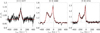 |
Fig. 1 Photosphere-subtracted profiles of the [O I] 5577, [O I] 6300, and [S II] 6731 lines in the ES 22.5 spectrum of RU Lup, and best-fitting combinations of Gaussian functions. |
Gaussian fits to forbidden emission lines in the ES 22.5 spectrum of RU Lup.
4 Discrete absorption components
RU Lup shows prominent emission in metallic species (Paper I). In this work, we focus on two strong resonance lines, the Na I D2 and the Ca II K lines. Both lines are components of a doublet: the Na I D doublet (D1 at λ = 5895.92 Å, D2 at λ = 5889.95 Å) and the Ca II H & K doublet (H at λ = 3968.47 Å, K at λ = 3933.66 Å). These lines were previously analyzed with UVES by Gahm et al. (2013), who identified a series of absorption components in their blue wings at velocities between 250 km s−1 and −100 km s−1. However, the very high resolution− of ESPRESSO enables a more detailed study of the line profiles. The line profiles are shown in Fig. 2 using the ES 22.5 spectrum as an example.
Figure 3 zooms in on the blue wing of the Ca II K and Na I D2 lines in the ES 22.5 spectrum. The broad (~350–400 km s−1) emission is locally attenuated in a set of discrete absorption components. These components are not photospheric because they are much broader than v sin i = 8.6 ± 1.4 km s−1 (Table C.1). Therefore, they originate in the outflowing gas, while the narrow absorption near ∼0 km s−1 arises from the interstellar medium (Pascucci et al. 2015). To systematize the analysis of these absorption features, we grouped them into three main components based on their centroid velocities in ES 22.5 and their persistence across spectra. We distinguish:
a high-velocity absorption component (HVA) that extends between −260 km s−1 and −180 km s−1,
a medium-velocity absorption component (MVA) that extends between −170 km s−1 and −130 km s−1,
a low-velocity absorption component (LVA) that extends between −100 km s−1 and −60 km s−1.
This classification is empirical and reflects the presence of preferred velocities in the absorbing gas. These velocity intervals were chosen to isolate the most prominent and recurrent absorption features, allowing for a meaningful comparison of their properties and variability.
The optical depth differs between features and between the Ca II K and Na I D2 lines. The HVA component is well defined only in Ca II K. The MVA is present in both species, although with a different velocity structure. It is more extended in Ca II K, and the profile minimum is more blueshifted in Ca II K than in Na I D2. The LVA is most clearly observed in Na I D2, where it appears as a broad and structured absorption feature. A weaker and narrower absorption is also present in the same velocity range in Ca II K, although its centroid is slightly more blueshifted. These differences indicate that these discrete features originate in distinct regions of the outflow. While neutral sodium likely probes a colder region of the wind, absorption in Ca II requires ionized material.
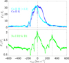 |
Fig. 2 Profiles of the Ca II H & K and Na I D2 & D1 doublets in the ES 22.5 spectrum of RU Lup. The Ca II H & K lines are plotted in velocity relative to their rest wavelengths. The Na I doublet is plotted in velocity relative to the rest wavelength of the D2 line. |
4.1 Variability
We used ESPRESSO spectra to study the variability of the discrete absorption components. Figure 4 shows the blue wings of the Ca II K and Na I D2 lines for all existing ESPRESSO observations of RU Lup.
The discrete components are well defined and structured in the 2022 spectra, whereas in 2021 they appear more complex and irregular, particularly in the Na I D2 line. The pronounced changes in shape and depth between the two 2021 spectra indicate a more dynamic wind, coincident with an epoch of higher accretion rate (Paper I and Wendeborn et al. 2024). This observation supports a direct link between the outflowing gas that produces these features and the accretion process.
A key qualitative difference lies in the morphology of the absorption. In 2021, the Na I D2 components exhibit blue-skewed profiles: single, asymmetric troughs whose depth varies monotonically across the profile. Such profiles naturally arise when the line of sight, ∆s, intersects an accelerating flow, so that the absorption samples a monotonic velocity gradient. The characteristic broadening from such a line-of-sight gradient is ∆vlos ≃ |dv/ds| ∆s. As the gas accelerates and expands, the absorption is expected to drift to higher blueshifts, consistent with the rapid, irregular variability observed in 2021.
In contrast, the absorption profiles in 2022 are often Gaussian-like or double-dipped, with remarkably stable centroids within an epoch. The MVA, for instance, remains centered at approximately −150 km s−1 throughout 2022. At this speed, the gas would travel ∼8 R⋆ per day (for R⋆ = 2.27 R⊙, Table C.1). Since we observed no significant velocity drifts over several days, this implies that the absorbing gas has already reached its terminal velocity.
Although the MVA centroid velocity is stable within each observing epoch, we detect a ∼−20 km s−1 shift in its centroid between 2021 and 2022 in both Ca II K and Na I D2. This suggests that the initial conditions of the outflow, such as the initial velocity or the launching angle, changed over time, possibly in response to the evolving accretion state of the system.
4.2 Comparison with forbidden emission lines
The HVA observed in the Ca II K line has the same velocity range as the HVC of the forbidden lines (see Fig. 5), indicating that the two features are connected. In Fig. 5, we supplemented the ES 22.5 observation (bottom panel) with two archival spectra. One is from the Echelle SpectroPolarimetric Device for the Observation of Stars (ESPaDOnS, middle panel) and is part of the spectra analyzed by Stock et al. (2022). The other is from UVES (top panel) and is included in the observations discussed by Stempels et al. (2007) and Gahm et al. (2008). The blueshifted extension of the [S II] 6731 line profile evolves in the same way as the Ca II K HVA. In particular, the two components drift toward higher blueshifted velocities, and the HVC becomes stronger relative to the continuum over time.
The two ESPRESSO epochs from 2021 are separated by ∆t = 9.06 days (Table A.1). Interpreting the variability of the discrete absorption components as a disturbance propagating along the flow at a characteristic velocity v 150 km s−1 (MVA in Fig. 3), the upper limit to the distance∼from the launching region is L ≲ v ∆t ≈ 0.78 AU. Conversely, the forbidden lines in RU Lup remain stable on such short baselines (e.g., Stock et al. 2022). Figure 5 shows that the HVC evolves on decadelong timescales, consistent with an extended, slowly varying jet component. This suggests that, although portions of the forbidden-line profiles fall within the LVA-MVA velocity range, these two tracers are formed in different regions of the outflow. The discrete components likely probe a column of gas close to the line-emitting region, whereas the forbidden lines integrate over an extended volume, sampling different streamlines and heights in the outflow.
4.3 Velocity decomposition of the absorbing gas
In 2022, the discrete absorption components in both Ca II K and Na I D2 are sometimes double-dipped, with stable centroids within each epoch (Sect. 4.1). Examples include the LVA in the ES 22.5 spectrum or the MVA in the ES 22.3 and 22.4 spectra. In this section, we use these double-dipped profiles to measure the rotational velocity of the outflow.
The velocity of the outflow can be described in cylindrical components (vr, vϕ, vz), with the stellar rotation axis aligned along  . The radial velocity of the gas is vrad = −vr cos ϕ sin i⋆ + vϕ sin ϕ sin i⋆ − vz cos i⋆ (Appendix E). At typical outflow temperatures (T ≲ 10 000 K), thermal broadening is only ∼1 km s−1, far below the observed ∼20–40 km s−1 widths of the components. In a nearly face-on geometry, to match the full absorption width in an accelerating flow, the (vertical) velocity gradient along the line of sight is given by ∆vlos ≈ |dvz/ds| ∆s cos i⋆. In CTTSs, MHD simulations of inner winds have shown that the flow accelerates on a scale of a few stellar radii (Romanova et al. 2009; Zanni & Ferreira 2013). Using a representative value of ∆s = RT ~ 0.02 AU, we require |dvz/ds| ∼ 103 km s−1 AU−1 to explain a line width of ∼20 km s−1. Such large gradients would imply blue-skewed troughs rather than symmetric profiles, with measurable centroid drifts as the sampled column moves along the line of sight. The expected acceleration is
 (2)
(2)
For vz = 150 km s−1, i⋆ = 16°, and previously computed |dvz/ds|, this predicts a drift of dvlos/dt ≈ 80 km s−1 day−1, which is not observed in 2022. Therefore, we conclude that a velocity gradient along the line of sight cannot be the dominant broadening mechanism in the absorption components in 2022.
Conversely, a finite azimuthal coverage, ∆ϕ, at a roughly fixed cylindrical radius produces a spread in vrad of ∆vrot ≃ 2vϕ sin i⋆ sin(∆ϕ/2). With i⋆ = 16° and a moderate azimuthal extent ∆ϕ = π/2, we find ∆vrot ≈ 0.4 vϕ. Therefore, toroidal velocities of ∼50 km s−1 are compatible with the observed line widths and naturally explain the stable centroids. Changes in vϕ and ∆ϕ modulate the width, while the centroid remains set by −vz cos i⋆.
Motivated by the above kinematic considerations, we modeled each discrete component as absorption from a sector of a narrow ring at cylindrical position (r, z) above the disk. Although the absorber is compact along the line of sight, it subtends a finite azimuthal range ϕ ∈ [ϕ1, ϕ2]. The resulting distribution of projected velocities can reproduce the Gaussian-like and double-dipped profiles observed in 2022. The assumption of a ring-like geometry is supported by MHD simulations, which show that disk winds tend to exhibit cylindrical symmetry even in fully three-dimensional setups (Romanova et al. 2009), and by the discrete nature of the observed components, which suggests localized ejection events rather than a continuous wind.
In the model, the gas is assumed to rotate and outflow, with a velocity vector decomposed into vertical (vz) and toroidal (vϕ) components. We assumed that the flow is predominantly in the vertical direction, so that  . The ring is limited between ϕ1 and ϕ2 in azimuth. The model has seven parameters: vz and vϕ, the angles ϕ1 and ϕ2, and the scaling parameters σ, τ0, and the covering factor (CF). A full description of the model parameters and the profile computation is given in Appendix E.
We used our model to fit the LVA of the ES 22.5 spectrum. We created a normalized profile using the red wing of the Na I D2 line as a model for the unabsorbed emission, as explained in Appendix D. We considered only the interval between −90 km s−1 and −15 km s−1 in the profile of Fig. D.1. Because of a degeneracy between τ0 and CF (Fig. E.2), we fixed CF = 1, assuming complete coverage of the emitting region. The resulting fit is shown in Fig. 6. The best fit has a reduced chi-square  of 1.5. The fit parameters are vz = 77.0±0.6 km s−1, vϕ = 29.2 ± 1.2 km s−1, ϕ1 = 100 ± 21°, ϕ2 = 163 ± 43°, τ0 = 0.126 ± 0.001, and σ = 4.39 ± 0.03 km s−1. The best-fit azimuthal limits suggest that the region is significantly extended in azimuth, with ∆ϕ = |ϕ2 − ϕ1| ≈ 3π/2.
We performed a similar analysis on the MVA component in the ES 22.3 and 22.4 spectra. In this case, we used the Na I D1 line instead of D2. This choice is due to the MVA of the D1 line lying is between the Na I D2 redshifted wing and the Na I D1 blueshifted wing, making it simple to identify a local continuum. Figure 7 presents the fit results. For the MVA in ES 22.3, the best fit parameters are vz = 152.3 ± 1.6 km s−1, vϕ = 55.2 ± 1.3 km s−1, ϕ1 = −160 ± 35°, ϕ2 = 90 ± 20°, τ0 = 0.112 ± 0.002, and σ = 6.74 ± 0.04 km s−1, with  . For the MVA in ES 22.4, the best fit parameters are vz = 151.5 ± 0.4 km s−1, vϕ = 34.8 ± 1.8 km s−1, ϕ1 = 165 ± 33°, ϕ2 = 113 ± 15°, τ0 = 0.106 ± 0.002, and σ = 4.45 ± 0.04 km s−1, with
  . The remaining components were not modeled because they do not exhibit the distinctive double-dipped morphology required for this fitting procedure.
Our ring model constrains the projected rotation V ≡ vϕ sin i⋆, so the uncertainty on i⋆ propagates directly into the inferred vϕ. In our fits, we fix i⋆ to its central value (16°; Table C.1). Holding V constant, differentiation gives  , with
  in radians. At i⋆ = 16° and
  (Table C.1), this corresponds to a relative uncertainty of 30% on vϕ. For example, for the LVA in ES 22.5, we obtain
  . This contribution of the inclination to the uncertainty in vz is comparable to the uncertainties of the formal fit. Therefore, we neglect it and quote the fit
  . Table 2 lists the values of vz and vϕ derived for the LVA and MVA components.
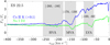 |
Fig. 3 Discrete absorption components observed for the Na I D2 (green) and Ca II K (blue) lines in the ES 22.5 spectrum of RU Lup. The shaded areas mark the velocity ranges where absorption is observed. |
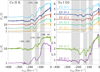 |
Fig. 4 Variability of the Ca II K and Na I D2 lines in the high resolution ESPRESSO spectra (Table A.1). The shaded areas mark the velocity ranges where absorption is observed. These ranges are the same as in Fig. 3 for the spectra from 2022, while the velocity range of the MVA is different in 2021, being [−150, −110] km s−1. |
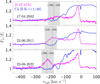 |
Fig. 5 Comparison of the Ca II K (blue) and [S II] 6731 (magenta) lines for a selection of RU Lup spectra. From top to bottom, the spectra are from UVES, ESPaDOnS, and ESPRESSO. The Ca II K lines were scaled by a factor of 1/40. The shaded areas trace the evolution of the two components, while the vertical lines mark the peak vrad of the HVC. |
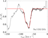 |
Fig. 6 Best-fit (red line) to the normalized absorption profile of the LVA component in the Na I D2 line from the ES 22.5 spectrum (black line). The profile is the same as that of Fig. D.1. Regions excluded from the fit are plotted in gray. |
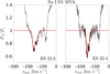 |
Fig. 7 Same as Fig. 6, but for the MVA component in the Na I D1 line from the ES 22.3 and ES 22.4 spectra. |
4.4 Launching radii and angular momentum removal
The distinct properties of the LVA and MVA components suggest that they originate in physically different regions of the outflow. The discrete nature of the components argues against an origin in a stellar wind. Such winds are expected to produce broad absorption profiles, as observed in the He I 10830 line (e.g., Edwards et al. 2006; Erkal et al. 2022). In contrast, the observations suggest a confined and transient origin, consistent with ejections from the disk.
Within the cold disk wind framework, the vertical velocity, vz, and the specific angular momentum, ℓ = rvϕ, depend on the launching radius, r0, and the magnetic lever arm, λ, defined as λ = (rA/r0)2. Here, rA is the Alfvén radius, that is, the point at which the poloidal velocity equals the Alfvén speed,  . The lever arm describes the efficiency of angular momentum extraction. Conservation of angular momentum beyond the Alfvén radius gives
 (3)
(3)
The terminal vz is linked to the Keplerian velocity at r0,  , as
, as
 (4)
(e.g., Ferreira et al. 2006). In this framework, different values of vz indicate different launching properties.
(4)
(e.g., Ferreira et al. 2006). In this framework, different values of vz indicate different launching properties.
Unlike forbidden emission lines imaged at high spatial resolution, the absorption features are spatially unresolved. Consequently, the cylindrical radius of the absorbing gas, rabs, and hence ℓ = rabsvϕ, cannot be directly determined. However, rabs can be related to the launching radius by calculating the intersection of the observer’s line of sight to the magnetosphere with a streamline that originates at r0 in the disk plane. Assuming that the streamline has an inclination θs and that the emission originates from a cylindrical radius rmag in the disk plane, the intersection yields
 (5)
(5)
(Appendix F.1). Together with the cold disk wind equations (Eqs. (3) and (4)), this equation allows the determination of r0, λ, and rabs as a function of the measured velocities, vz and vϕ, and the parameters i⋆, θs, and rmag. By introducing  , we can obtain r0 from the cubic equation
 (6)
(6)
Details of the derivation are provided in Appendix F.2.
We studied the families of solutions by plotting r0 as a function of rmag for a grid of θs values at fixed i⋆ = 16°. Details are reported in Appendix F.3. The key result is that imposing an upper bound on rabs (≲L sin i⋆ with L = 1 AU) limits the launching radius to r0 ≲ 6.76 R⋆ for both components. Using the measured vz and the cold disk wind relations then yields λLVA ∈ [1.56, 1.93] and λMVA ∈ [1.75, 3.20], with λLVA < λMVA at a given r0. An upper bound on the specific angular momentum of each component follows from the upper limit on rabs and the measured vϕ. Using the central values of vϕ, we obtain ℓLVA ≲ 8.1 AU km s−1, ℓMVA(ES 22.3) ≲ 15.2 AU km s−1, and ℓMVA(ES 22.4) ≲ 9.6 AU km s−1.
4.5 Rate of mass loss
To quantify the contribution of the different components of the outflow to the mass and angular momentum budget of the system, we estimated the mass-loss rate associated with the LVA and MVA. The total mass-loss rate can be expressed as
 (7)
where µ ≈ 1.3 is the mean molecular weight for a gas of solar composition, mH is the mass of the hydrogen atom, nH is the hydrogen number density, A is the area through which the gas flows, and vz is the vertical velocity of the absorbing material. Since these features are observed in absorption, we simplify the expression by relating the hydrogen number density to the column density as nH = NH/∆s, where ∆s is the extent of the absorbing gas along the line of sight. The area, A, is computed by assuming the same ring-like geometry described in Sect. 4.3. The ring is located at the absorbing radius, rabs, has a radial thickness ∆r, and an azimuthal extent ∆ϕ = |ϕ2 − ϕ1|. Therefore, the area of the absorbing region is A = ∆ϕrabs ∆r. The radial thickness is related to the line-of-sight extent by ∆r = ∆s sin i⋆, where i⋆ is the system inclination (see Fig. E.1). Substituting into the previous expressions, we obtain
(7)
where µ ≈ 1.3 is the mean molecular weight for a gas of solar composition, mH is the mass of the hydrogen atom, nH is the hydrogen number density, A is the area through which the gas flows, and vz is the vertical velocity of the absorbing material. Since these features are observed in absorption, we simplify the expression by relating the hydrogen number density to the column density as nH = NH/∆s, where ∆s is the extent of the absorbing gas along the line of sight. The area, A, is computed by assuming the same ring-like geometry described in Sect. 4.3. The ring is located at the absorbing radius, rabs, has a radial thickness ∆r, and an azimuthal extent ∆ϕ = |ϕ2 − ϕ1|. Therefore, the area of the absorbing region is A = ∆ϕrabs ∆r. The radial thickness is related to the line-of-sight extent by ∆r = ∆s sin i⋆, where i⋆ is the system inclination (see Fig. E.1). Substituting into the previous expressions, we obtain
 (8)
(8)
For both components, we measured an azimuthal span ∆ϕ ≈ 3π/2 (Sect. 4.3) and we adopt the conservative upper limit rabs ≲ 0.276 AU (Appendix F.3). Thus, the mass-loss rate of the two components differs due to their measured NH and vz. Our estimate of NH is derived from the equivalent width of the Na I D lines, as described in Appendix D.
For the LVA, the absence of Ca II absorption suggests that the absorbing gas is predominantly neutral, so that NH follows directly from Na I under the assumption of solar abundances. We obtain NH = 5.49 × 1017 cm−2 (Appendix D) and vz = 77.0 km s−1 (Sect. 4.3). This corresponds to  .
.
For the MVA, the strength of Ca II absorption suggests that sodium in the absorbing gas is predominantly ionized, so NH must be inferred by correcting Na I for excitation and ionization effects. In Appendix D we estimate NH = 1.16 × 10¹⁸ χ−1 cm−2, where χ = NNaI/NNa is the fraction of sodium atoms in the neutral state. Using vz = 151.5 km s−1 (Sect. 4.3), we find  .
.
The ionization level of the MVA is further supported by values of χ predicted by the Saha equation (Fig. 8). For plausible temperatures reached in the inner disk close to the star (T ∼ 3000 K), the neutral sodium fraction lies in the range 10−3 − 10−5, implying that the measured Na I absorption likely traces only a small fraction of the total gas column. Nisini et al. (2018) found that in CTTSs, the forbidden lines trace winds with  . If the discrete absorption components probe similar mass-loss channels, adopting
  for RU Lup implies a neutral sodium fraction of χ ∼ 3.3 × 10⁻⁴.
Summary of derived properties for the LVA and MVA components.
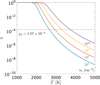 |
Fig. 8 Neutral fraction of sodium (χ) as a function of T, computed using the Saha equation for different values of ne. The dash-dotted line marks the critical neutral fraction χb required for the MVA wind torque to balance the accretion torque (see Sect. 5.5). |
5 Discussion
The discrete absorption components and their connection with the forbidden lines provide important insights into the structure of the RU Lup outflow. Here, we outline the implications of our observations on the physics of the MHD-driven wind of RU Lup and, by extension, of CTTSs in general. Table 2 summarizes the properties derived for the LVA and MVA.
A variety of MHD simulations have shown that coexisting winds can be launched from different regions of the star–disk system (e.g., Ferreira et al. 2006). Extended magneto-centrifugal disk winds, driven from the disk surface over a range of radii, naturally produce an “onion-like” flow in which the inner streamlines have higher poloidal velocity. At the same time, magnetospheric wind models (e.g., Romanova et al. 2009; Kurosawa & Romanova 2012) suggest that matter is expelled from the star–disk boundary near the truncation radius. Moreover, any stellar wind accelerated along open stellar field lines might produce a high-velocity component (e.g. Matt & Pudritz 2005a). Overall, simulations predict the coexistence of a disk wind, a magnetospheric wind, and a stellar wind. Each mechanism dominates a different region of the outflow, producing a multilayered structure, which has been confirmed by observations (e.g., Bacciotti et al. 2002; Pyo et al. 2006; Krist et al. 2008; Bacciotti et al. 2025).
5.1 Origin of the broad Ca II emission
In Paper I, we showed that the rich emission spectrum of RU Lup is formed in the accretion flow that leaves the disk at RT. The Na I D lines have excitation conditions and line profiles similar to those of the neutral metallic lines studied previously, such as the Fe I 5447 line, indicating a similar formation mechanism, as discussed in Paper I.
Conversely, Fig. 3 shows that the Ca II H & K lines are much broader than the Na I D lines, with detectable emission up to ∼−400 km s−1. Coffey et al. (2007) observed the jet of the CTTS DG Tau with the Hubble Space Telescope Imaging Spectrograph (HST/STIS) in the near-ultraviolet (NUV) by placing the slit at a distance of 0.3′′ from the star, corresponding to a de-projected distance along the jet of 68 AU. They showed that the blue wing emission of the Mg II h & k doublet in DG Tau forms within the jet. Comparing their observation with an HST spectrum of DG Tau with a 2′′ coverage centered on the star (Ardila et al. 2002), in which the Mg II k line showed a deep blueshifted absorption, Coffey et al. (2007) concluded that the jet was both absorbing and emitting in Mg II (Fig. 9 of their paper). The Mg II h & k doublet is analogous to the Ca II H & K doublet (hence the same denomination). This similarity suggests that the wings of the Ca II H & K doublet lines also originate in the jet and that the absorption components observed in the Ca II K line are a manifestation of the jet self-absorption.
5.2 HVA component: Jet knot at large scale
The similar velocity structure between the Ca II HVA and the HVC of the forbidden lines (see Fig. 5) indicates a common origin. This has been previously observed for the CTTS V1331 Cyg by Petrov et al. (2014), who described the discrete absorption components as “shell profiles.”
For RU Lup, Whelan et al. (2021) show that the HVC component of the [S II] 6371 line is formed in a “knot” of the outflow at ∼55 AU along the outflow position angle (PA). The knot is likely formed due to a shock within the jet, in which ionized atoms recombine in the post-shock region (e.g., Hartigan et al. 1995). The observed velocity sub-structure in the Ca II HVA is compatible with a formation in a shocked region, where the flow is likely turbulent and parcels of gas could have a local velocity component relative to the bulk velocity of the knot.
Unlike the LVA and MVA, which trace the outflow close to the launching region, the HVA is associated with the large-scale structure of the jet, which has low density and is also observed in the forbidden lines. For the HVA, the line width likely does not represent the toroidal velocity in the flow. The absence of an HVA in Na I indicates that sodium is fully ionized. Similarly, hydrogen is expected to be ionized, implying nH ≈ ne. Given the lower density of the outflow, the column required to produce such an optically thick absorption component must be significantly greater than in the regions responsible for the other two absorption features. Consequently, the observed velocity range may result from the gradient in vz along the line of sight, or from turbulent broadening within the shocked region.
5.3 LVC-BC: Conical wind
The HVC and LVC-NC components of the forbidden lines have a known origin (Whelan et al. 2021, and Sect. 3). Here, we focus on the newly identified LVC-BC, which is most evident in the [O I] 5577 line. This component is blueshifted and broad, with a profile that extends to redshifted velocities. These properties suggest the presence of rotation and outflowing motion in a relatively compact region. Using the FWHM of the line, we suggest that the outflow is launched from the inner disk, close to the disk truncation radius, RT ≈ 2 R⋆ = 0.02 AU (Table C.1).
The LVC-BC is also detected in the [O I] 6300 and [S II] 6731 lines, and their profiles suggest a layered wind structure. The [O I] 6300 component is broader and more blueshifted than [O I] 5577, indicating that it traces material that has reached higher poloidal velocities and developed a stronger toroidal component farther out in the wind. In contrast, the [S II] 6731 line, which has a much lower critical density, shows only a narrow, blueshifted component without a red wing, pointing to emission from the outermost regions of the wind, where rotation has largely dissipated and poloidal motion dominates. The three lines reveal a stratified MHD wind: as gas is launched and accelerates away from the disk, it becomes progressively less dense, gains a toroidal velocity component, and ultimately reaches a regime dominated by poloidal flow.
The properties of the LVC-BC fit the description of the conical wind observed in the MHD simulations performed by Romanova et al. (2009). This type of outflow is launched from a narrow region of the inner disk between RT and Rco, where the stellar magnetosphere interacts with the inner disk.
5.4 LVA and MVA components: Ejections from the inner disk
The kinematic constraints derived in Sect. 4.4 and Appendix F.3 suggest that the LVA and MVA trace outflows launched from the inner disk at r0 ≲ 6.76 R⋆. Using the measured vz in the cold disk wind approximation (Eq. (4)) yields λ intervals of λLVA ∈ [1.56, 1.93] and λMVA ∈ [1.75, 3.20], where the lower limits assume r0 ≥ R⋆. The geometry confines the streamline inclination to θs ∼ 12°–14°.
Despite similar kinematic properties, the two discrete absorption components appear to have different ionization stages. The LVA is detected only in Na I, whereas the MVA appears in both Na I and Ca II. After correcting the Na I column density for ionization, this suggests that the MVA carries a larger mass flux. To interpret this in the framework of magneto–centrifugal disk winds, we introduce the ejection efficiency
 (9)
which measures the fractional mass loading of the wind per logarithmic interval in launching radius (Casse & Ferreira 2000a). In the cold disk wind theory, the magnetic lever arm relates to ξ by λ ≃ 1 − 1/2ξ (Ferreira 1997), so that similar lever arms imply similar ejection efficiencies. The total wind mass-loss rate from an annulus [rin, rout] is
(9)
which measures the fractional mass loading of the wind per logarithmic interval in launching radius (Casse & Ferreira 2000a). In the cold disk wind theory, the magnetic lever arm relates to ξ by λ ≃ 1 − 1/2ξ (Ferreira 1997), so that similar lever arms imply similar ejection efficiencies. The total wind mass-loss rate from an annulus [rin, rout] is
 (10)
(e.g., Casse & Ferreira 2000a). Given similar values of ξ, a three-order-of-magnitude difference in
(10)
(e.g., Casse & Ferreira 2000a). Given similar values of ξ, a three-order-of-magnitude difference in  cannot be explained by a plausible difference in ln(rout/rin) alone. This indicates that LVA and MVA have comparable mass fluxes, hence similar ionization levels. In this scenario, the non-detection of the LVA in Ca II can be explained if the LVA covers a very small portion of the Ca II emitting background, leading to an underestimated ionization level and thus
  . This is plausible if the low-velocity portion of the Ca II emission does not arise primarily in the magnetosphere but in a region of the inner wind closer to the axis, as suggested in Sect. 5.1. We quantify this scenario in Appendix G, where we show that if the Ca II emission arises in an inner, axial outflow, the absorbing gas can be arranged in two broader shells: the MVA just outside the emitting region and the LVA further out. In this picture, our line of sight to the emitting region traverses the MVA layer, yielding a large line–emitter covering fraction but a small continuum covering, producing deep absorption that remains above the continuum. Conversely, the LVA crosses the continuum emission but largely misses the Ca II emitter, so absorption at the LVA velocity is diluted to a few percent.
The ejection index, ξ, measures the local efficiency of mass loss from the accretion disk into the wind, reflecting how rapidly  decreases with r. From the measured λ, we infer ξLVA ≈ 0.54–0.89 and ξMVA ≈ 0.23–0.67. These values point to “warm” MHD winds characterized by efficient mass loading (Casse & Ferreira 2000b). Such high values of ξ exceed those typical of cold MHD winds, which usually exhibit ξ ~ 0.01 (Ferreira 1997), indicating minimal mass loading. Warm disk wind models invoke surface heating mechanisms that raise the gas thermal energy and increase the pressure scale height, thereby enhancing the vertical pressure gradient at the disk surface. This yields stronger mass ejection, leading to higher ξ values in the range 0.1–0.3 or more, depending on heating strength (Casse & Ferreira 2000b; Ferreira & Casse 2004). Our derived values suggest winds with significant thermal energy contributions, consistent with heated disk atmospheres or episodic magnetospheric ejections, as discussed in MHD models (Ferreira et al. 2006; Zanni & Ferreira 2013).
The MVA exhibits a vertical velocity approximately twice that of the LVA. If λ were the same for both components, a purely inward shift of the footpoint would require r0 to decrease by a factor of four. Assuming the LVA launches at our inferred upper limit (r0 = 6.76 R⋆) yields r0 = 1.69 R⋆ for the MVA, which is too close to the stellar surface. Thus, launching closer to the star cannot fully explain the observed vz of the MVA, suggesting that the MVA either traces streamlines with a larger lever arm λ or has a non-negligible enthalpy at its base. In the latter case, Eq. (4) is modified to
 (11)
where β parametrizes the additional enthalpy available to accelerate the gas (Ferreira et al. 2006). Assuming a nearly uniform λ across the inner disk and treating the LVA as a cold wind (βLVA = 0), the β required to reach the observed vz of the MVA is
(11)
where β parametrizes the additional enthalpy available to accelerate the gas (Ferreira et al. 2006). Assuming a nearly uniform λ across the inner disk and treating the LVA as a cold wind (βLVA = 0), the β required to reach the observed vz of the MVA is  . Adopting λ in the LVA range, we find βMVA ∈ [0.4–0.9] for r0 = 2 R⋆ and βMVA ∈ [0.6–1.4] for r0 = 3 R⋆. Allowing the LVA to be warm (βLVA > 0) proportionally reduces the required βMVA, but the qualitative conclusion remains: either a larger λ or additional pressure support is needed to justify the higher observed vz of the MVA.
In summary, a consistent scenario is that the inner disk launches a warm, magneto–centrifugal disk wind with a narrow spread in the opening angle (θs ∼ 12°–14°), producing two persistent absorption components, the LVA and MVA. The different observed velocities can be explained if the MVA is launched from smaller r0, close to RT, and has either a higher λ or a higher heat content at its base. The observed differences among the absorption components indicate a velocity-stratified disk wind near the star, disfavoring an X-wind scenario (Shu et al. 1994), in which the outflow is launched from a narrow annulus at the truncation radius and therefore carries a single specific angular momentum and lever arm.
5.5 Spinning-down RU Lup: Efficiency of magnetospheric ejections
A main result of Paper I was the determination of the disk truncation radius, RT, of RU Lup from the analysis of the light curve obtained with the Transiting Exoplanet Survey Satellite (TESS; Ricker et al. 2014). We derived RT ≈ 2 R⋆ and showed that R varies with the accretion rate,  . We estimated
  during the TESS Sector 65 observation. Together with M⋆ (Table C.1), these measures allow us to compute the accretion torque,
 (12)
(e.g., Matt & Pudritz 2005b; Pantolmos et al. 2020). We obtain τacc = 9.46 × 1043 g cm2 s−2 or, in more convenient units, τacc = 3.2 × 10⁻⁷ M⊙ yr−1 AU km s−1.
(12)
(e.g., Matt & Pudritz 2005b; Pantolmos et al. 2020). We obtain τacc = 9.46 × 1043 g cm2 s−2 or, in more convenient units, τacc = 3.2 × 10⁻⁷ M⊙ yr−1 AU km s−1.
This torque spins up the star on a characteristic timescale tacc = I⋆Ω⋆/τacc, where  is the stellar moment of inertia and Ω⋆ = 2π/P⋆ is the stellar angular velocity. Using P⋆ = 3.71 days (Table C.1), we derive tacc ≈ 3.57 × 10⁴ years for RU Lup. Since the star has an age of ∼2–3 Myr (Herczeg et al. 2005), it should already rotate at break-up velocity. This implies the presence of an efficient spin-down mechanism that removes angular momentum from the star-disk system via outflows.
In Sect. 5.4, we showed that the MVA likely traces an ejection launched from very small r0, in a region of the disk that is magnetically connected to the star. Its kinematics appears to respond to the accretion state: the toroidal velocity is higher in ES 22.3 than in ES 22.4 (Table 2), and Paper I reports a larger veiling fraction in ES 22.3, indicating stronger accretion. This correlation supports the idea that the outflow traced by the MVA may act as an efficient channel for angular momentum removal from the star-disk system. Moreover, our analysis indicates that the winds traced by the LVA and MVA are substantially mass-loaded and warm, as expected for outflows launched from the inner disk. This picture is consistent with models in which the magnetosphere episodically ejects blobs of gas that contribute to stellar spin-down during enhanced accretion phases (e.g., Zanni & Ferreira 2013). In this framework, our measurements of  and ℓ allow us to quantitatively address the spin-down problem.
To assess whether the outflow traced by the MVA can counteract the spin-up torque from accretion, we express the wind torque as a function of the fraction of sodium in the neutral state, χ. Combining  with ℓ obtained from the ES 22.3 spectrum (Table 2), the upper limit on the MVA torque
  ℓ is 5.02 × 10⁻¹¹ χ−1 M⊙ yr−1 AU km s−1.
Balancing τMVA with the accretion torque requires a neutral fraction χb ≳ 1.57 × 10⁻⁴, corresponding to  , which is ∼20% of
  . If the neutral fraction increases to χ = 3.3 × 10⁻⁴, yielding
  (Sect. 4.5), the MVA wind still carries away ≲50% of the accretion torque, indicating a substantial contribution to angular momentum removal. Together with the modest lever arm, these results reinforce a warm, mass-loaded disk wind solution capable of regulating the stellar spin.
6 Conclusions
In this work, we used the high resolution ESPRESSO spectra of RU Lup, obtained as part of the PENELLOPE program (Manara et al. 2021), to study the outflow structure of this strongly accreting CTTS. The observations trace the outflow close to the launching region and constrain the spin-down mechanism. Specifically, we combined information extracted from the forbidden emission lines with a study of absorption components in the permitted resonance lines of the Na I D1&D2 and Ca II H&K doublets. Figure 9 illustrates the multi-component outflow and the locations of the observed absorptions.
The main results are summarized as follows:
The LVC–BC of the forbidden emission lines traces an MHD wind launched from the inner disk, which we identify with the conical wind predicted by MHD simulations (Romanova et al. 2009).
The HVA component is connected to the HVC of the forbidden lines; both originate in the low-density outer jet at distances ≳50 AU;
In the 2022 ESPRESSO spectra of RU Lup, the MVA and LVA sometimes display a double-dipped absorption consistent with rotation. We developed a method to disentangle the vertical (vz) and toroidal (vϕ) velocities in these DACs and to infer the launching radius r0, magnetic lever arm λ, and mass-loss rate
 ;
;The LVA and MVA trace a warm, highly mass-loaded disk wind launched from the inner disk (r0 ≲ 6.76 R⋆) with low magnetic lever arms (Casse & Ferreira 2000b). The two components mainly differ in their observed poloidal velocities (vz is about twice as large in the MVA as in the LVA) and in the weakness of the LVA in Ca II;
The LVA is explained as an outer absorbing shell with λLVA ∈ [1.56, 1.93] and a low covering of the Ca II line-emitting region. We attribute its weakness in Ca II to geometry (small line-emitter covering fraction) rather than lower ionization compared to the MVA;
The MVA traces a distinct inner wind layer that forms near the truncation radius RT, whose higher vz is compatible with either a slightly larger lever arm, λMVA ∈[1.75, 3.20], or with additional thermal support at the base, parametrized by β ∈ [0.4, 0.9];
The LVA-MVA contrast arises from different covering fractions and stratification in a warm disk wind launched across a narrow annulus near RT, disfavoring a pure X-wind scenario (e.g., Shu et al. 1994);
We evaluated the MVA wind torque as a function of the sodium neutral fraction χ, and show that the MVA removes a substantial fraction of the accretion spin-up torque for plausible ionization levels in the inner disk.
Future studies should aim to extend this analysis to other systems. While the low inclination of RU Lup provides a direct view of the outflow, systems observed at higher inclinations are expected to exhibit larger radial velocity gradients due to toroidal motion, offering the advantage of more effectively separating the double-dipped structure of the absorption components. Additionally, time-resolved spectroscopic observations over various timescales would enable detailed investigations of the variability of the different outflow components and their connection to the accretion process.
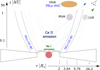 |
Fig. 9 Sketch of the outflow structure of RU Lup inferred from our analysis. The figure is not to scale. |
Acknowledgements
The authors thank the anonymous referee for their critical review of this manuscript. This work has been supported by Deutsche Forschungsgemeinschaft (DFG) in the framework of the YTTHACA Project (469334657) under the project codes STE 1068/9-1 and MA 8447/1-1. AF acknowledges financial support from the Large Grant INAF 2022 “YSOs Outflows, Disks and Accretion: towards a global framework for the evolution of planet forming systems” (YODA). CFM and JCW are funded by the European Union (ERC, WANDA, 101039452). Views and opinions expressed are however those of the author(s) only and do not necessarily reflect those of the European Union or the European Research Council Executive Agency. Neither the European Union nor the granting authority can be held responsible for them. JFG was supported by Fundação para a Ciência e Tecnologia (FCT) through the research grants UIDB/04434/2020 and UIDP/04434/2020. The authors acknowledge the use of the electronic bibliography maintained by the NASA/ADS1 system.
References
- Alcalá, J. M., Manara, C. F., Natta, A., et al. 2017, A&A, 600, A20 [NASA ADS] [CrossRef] [EDP Sciences] [Google Scholar]
- Ardila, D. R., Basri, G., Walter, F. M., Valenti, J. A., & Johns-Krull, C. M. 2002, ApJ, 567, 1013 [NASA ADS] [CrossRef] [Google Scholar]
- Armeni, A., Stelzer, B., Frasca, A., et al. 2024, A&A, 690, A225 [NASA ADS] [CrossRef] [EDP Sciences] [Google Scholar]
- Asplund, M., Grevesse, N., Sauval, A. J., & Scott, P. 2009, A&A, 47, 481 [CrossRef] [Google Scholar]
- Bacciotti, F., Ray, T. P., Mundt, R., Eislöffel, J., & Solf, J. 2002, ApJ, 576, 222 [Google Scholar]
- Bacciotti, F., Nony, T., Podio, L., et al. 2025, A&A, 704, A157 [NASA ADS] [CrossRef] [EDP Sciences] [Google Scholar]
- Bacon, R., Accardo, M., Adjali, L., et al. 2010, SPIE Conf. Ser., 7735, 773508 [Google Scholar]
- Balbus, S. A., & Hawley, J. F. 1991, ApJ, 376, 214 [Google Scholar]
- Banzatti, A., & Pontoppidan, K. M. 2015, ApJ, 809, 167 [NASA ADS] [CrossRef] [Google Scholar]
- Banzatti, A., Pascucci, I., Edwards, S., et al. 2019, ApJ, 870, 76 [Google Scholar]
- Birney, M., Whelan, E. T., Dougados, C., et al. 2024, A&A, 692, L5 [NASA ADS] [CrossRef] [EDP Sciences] [Google Scholar]
- Bouvier, J., Alencar, S. H. P., Harries, T. J., Johns-Krull, C. M., & Romanova, M. M. 2007, in Protostars and Planets V, eds. B. Reipurth, D. Jewitt, & K. Keil, 479 [Google Scholar]
- Bouvier, J., Matt, S. P., Mohanty, S., et al. 2014, in Protostars and Planets VI, eds. H. Beuther, R. S. Klessen, C. P. Dullemond, & T. Henning, 433 [Google Scholar]
- Campbell-White, J., Manara, C. F., Benisty, M., et al. 2023, ApJ, 956, 25 [NASA ADS] [CrossRef] [Google Scholar]
- Casse, F., & Ferreira, J. 2000a, A&A, 353, 1115 [NASA ADS] [Google Scholar]
- Casse, F., & Ferreira, J. 2000b, A&A, 361, 1178 [NASA ADS] [Google Scholar]
- Coffey, D., Bacciotti, F., Ray, T. P., Eislöffel, J., & Woitas, J. 2007, ApJ, 663, 350 [NASA ADS] [CrossRef] [Google Scholar]
- Dekker, H., D'Odorico, S., Kaufer, A., Delabre, B., & Kotzlowski, H. 2000, SPIE Conf. Ser., 4008, 534 [NASA ADS] [Google Scholar]
- Edwards, S., Cabrit, S., Strom, S. E., et al. 1987, ApJ, 321, 473 [Google Scholar]
- Edwards, S., Fischer, W., Hillenbrand, L., & Kwan, J. 2006, ApJ, 646, 319 [Google Scholar]
- Ercolano, B., & Pascucci, I. 2017, Roy. Soc. Open Sci., 4, 170114 [Google Scholar]
- Erkal, J., Manara, C. F., Schneider, P. C., et al. 2022, A&A, 666, A188 [NASA ADS] [CrossRef] [EDP Sciences] [Google Scholar]
- Espaillat, C. C., Herczeg, G. J., Thanathibodee, T., et al. 2022, AJ, 163, 114 [NASA ADS] [CrossRef] [Google Scholar]
- Fang, M., Pascucci, I., Edwards, S., et al. 2018, ApJ, 868, 28 [NASA ADS] [CrossRef] [Google Scholar]
- Ferreira, J. 1997, A&A, 319, 340 [Google Scholar]
- Ferreira, J., & Casse, F. 2004, ApJ, 601, L139 [NASA ADS] [CrossRef] [Google Scholar]
- Ferreira, J., Dougados, C., & Cabrit, S. 2006, A&A, 453, 785 [NASA ADS] [CrossRef] [EDP Sciences] [Google Scholar]
- Frasca, A., Biazzo, K., Lanzafame, A. C., et al. 2015, A&A, 575, A4 [NASA ADS] [CrossRef] [EDP Sciences] [Google Scholar]
- Gahm, G. F., Walter, F. M., Stempels, H. C., Petrov, P. P., & Herczeg, G. J. 2008, A&A, 482, L35 [NASA ADS] [CrossRef] [EDP Sciences] [Google Scholar]
- Gahm, G. F., Stempels, H. C., Walter, F. M., Petrov, P. P., & Herczeg, G. J. 2013, A&A, 560, A57 [NASA ADS] [CrossRef] [EDP Sciences] [Google Scholar]
- Gaia Collaboration (Brown, A. G. A., et al.) 2021, A&A, 649, A1 [NASA ADS] [CrossRef] [EDP Sciences] [Google Scholar]
- GRAVITY Collaboration (Perraut, K., et al.) 2021, A&A, 655, A73 [NASA ADS] [CrossRef] [EDP Sciences] [Google Scholar]
- Hartigan, P., Edwards, S., & Ghandour, L. 1995, ApJ, 452, 736 [Google Scholar]
- Hartmann, L. 2008, Accretion Processes in Star Formation, 2nd edn., Cambridge Astrophysics (Cambridge University Press) [Google Scholar]
- Hartmann, L., & Stauffer, J. R. 1989, AJ, 97, 873 [Google Scholar]
- Hartmann, L., Herczeg, G., & Calvet, N. 2016, A&A, 54, 135 [Google Scholar]
- Herczeg, G. J., Walter, F. M., Linsky, J. L., et al. 2005, AJ, 129, 2777 [NASA ADS] [CrossRef] [Google Scholar]
- Hirth, G. A., Mundt, R., & Solf, J. 1997, A&A, 126, 437 [Google Scholar]
- Krist, J. E., Stapelfeldt, K. R., Hester, J. J., et al. 2008, AJ, 136, 1980 [NASA ADS] [CrossRef] [Google Scholar]
- Kurosawa, R., & Romanova, M. M. 2012, MNRAS, 426, 2901 [NASA ADS] [CrossRef] [Google Scholar]
- Kwan, J., & Tademaru, E. 1988, ApJ, 332, L41 [NASA ADS] [CrossRef] [Google Scholar]
- Lesur, G. R. J. 2021, A&A, 650, A35 [NASA ADS] [CrossRef] [EDP Sciences] [Google Scholar]
- Manara, C. F., Frasca, A., Venuti, L., et al. 2021, A&A, 650, A196 [NASA ADS] [CrossRef] [EDP Sciences] [Google Scholar]
- Manara, C. F., Ansdell, M., Rosotti, G. P., et al. 2023, in Protostars and Planets VII, 534, eds. S. Inutsuka, Y. Aikawa, T. Muto, K. Tomida, & M. Tamura, 539 [NASA ADS] [Google Scholar]
- Matt, S., & Pudritz, R. E. 2005a, ApJ, 632, L135 [Google Scholar]
- Matt, S., & Pudritz, R. E. 2005b, MNRAS, 356, 167 [NASA ADS] [CrossRef] [Google Scholar]
- Mayor, M., Pepe, F., Queloz, D., et al. 2003, The Messenger, 114, 20 [NASA ADS] [Google Scholar]
- Natta, A., Testi, L., Alcalá, J. M., et al. 2014, A&A, 569, A5 [NASA ADS] [CrossRef] [EDP Sciences] [Google Scholar]
- Nisini, B., Antoniucci, S., Alcalá, J. M., et al. 2018, A&A, 609, A87 [EDP Sciences] [Google Scholar]
- Osterbrock, D. E., & Ferland, G. J. 2006, Astrophysics of Gaseous Nebulae and Active Galactic Nuclei (University Science Books) [Google Scholar]
- Pantolmos, G., Zanni, C., & Bouvier, J. 2020, A&A, 643, A129 [NASA ADS] [CrossRef] [EDP Sciences] [Google Scholar]
- Pascucci, I., Edwards, S., Heyer, M., et al. 2015, ApJ, 814, 14 [Google Scholar]
- Pascucci, I., Cabrit, S., Edwards, S., et al. 2023, in Astronomical Society of the Pacific Conference Series, 534, Protostars and Planets VII, eds. S. Inutsuka, Y. Aikawa, T. Muto, K. Tomida, & M. Tamura, 567 [NASA ADS] [Google Scholar]
- Pepe, F., Cristiani, S., Rebolo, R., et al. 2021, A&A, 645, A96 [NASA ADS] [CrossRef] [EDP Sciences] [Google Scholar]
- Petrov, P. P., Kurosawa, R., Romanova, M. M., et al. 2014, MNRAS, 442, 3643 [Google Scholar]
- Pyo, T.-S., Hayashi, M., Kobayashi, N., et al. 2006, Adaptive Optics Spectroscopy of the [Fe II] Outflows from HL Tauri and RW Aurigae [Google Scholar]
- Ray, T., Dougados, C., Bacciotti, F., Eislöffel, J., & Chrysostomou, A. 2007, in Protostars and Planets V, eds. B. Reipurth, D. Jewitt, & K. Keil, 231 [Google Scholar]
- Ricker, G. R., Winn, J. N., Vanderspek, R., et al. 2014, SPIE Conf. Ser., 9143, 914320 [Google Scholar]
- Rigliaco, E., Pascucci, I., Gorti, U., Edwards, S., & Hollenbach, D. 2013, ApJ, 772, 60 [NASA ADS] [CrossRef] [Google Scholar]
- Roman-Duval, J., Proffitt, C. R., Taylor, J. M., et al. 2020, RNAAS, 4, 205 [NASA ADS] [Google Scholar]
- Romanova, M. M., Ustyugova, G. V., Koldoba, A. V., & Lovelace, R. V. E. 2009, MNRAS, 399, 1802 [Google Scholar]
- Shu, F., Najita, J., Ostriker, E., et al. 1994, ApJ, 429, 781 [Google Scholar]
- Simon, M. N., Pascucci, I., Edwards, S., et al. 2016, ApJ, 831, 169 [Google Scholar]
- Smette, A., Sana, H., Noll, S., et al. 2015, A&A, 576, A77 [NASA ADS] [CrossRef] [EDP Sciences] [Google Scholar]
- Sperling, T., Eislöffel, J., Manara, C. F., et al. 2024, A&A, 687, A54 [NASA ADS] [CrossRef] [EDP Sciences] [Google Scholar]
- Spitzer, L. 1998, Physical Processes in the Interstellar Medium [Google Scholar]
- Stempels, H. C., Gahm, G. F., & Petrov, P. P. 2007, A&A, 461, 253 [NASA ADS] [CrossRef] [EDP Sciences] [Google Scholar]
- Stock, C., McGinnis, P., Caratti o Garatti, A., Natta, A., & Ray, T. P. 2022, A&A, 668, A94 [NASA ADS] [CrossRef] [EDP Sciences] [Google Scholar]
- Weber, M. L., Ercolano, B., Picogna, G., Hartmann, L., & Rodenkirch, P. J. 2020, MNRAS, 496, 223 [NASA ADS] [CrossRef] [Google Scholar]
- Wendeborn, J., Espaillat, C. C., Lopez, S., et al. 2024, ApJ, 970, 118 [Google Scholar]
- Whelan, E. T., Pascucci, I., Gorti, U., et al. 2021, ApJ, 913, 43 [NASA ADS] [CrossRef] [Google Scholar]
- Zanni, C., & Ferreira, J. 2013, A&A, 550, A99 [NASA ADS] [CrossRef] [EDP Sciences] [Google Scholar]
Appendix A Log of spectroscopic observations
Table A.1 reports the spectroscopic observations used in this work.
Log of the spectroscopic observations.
Appendix B Photospheric subtraction in the forbidden emission lines
The line profiles of the forbidden emission lines of RU Lup are severely blended with the absorption lines from the photosphere of the star. To study the kinematics of the outflow, it is important to remove the stellar contribution from the profiles of the forbidden lines. To this end, we used the template spectrum that we have identified in Paper I as best fitting the photospheric spectrum of RU Lup. The properties of the template were obtained using the ROTFIT code (Frasca et al. 2015), which uses a library of High Accuracy Radial velocity Planet Searcher (HARPS, Mayor et al. 2003) spectra from the ESO Archive to fit the photospheric spectrum. The details of the procedure to obtain the template are reported in Paper I.
For each emission line, we adjusted the veiling fraction (VF) in its vicinity to match the depth of the photospheric lines. The procedure and the result of the photospheric subtraction are shown in Fig. B.1. Due to the effect of line filling emission in the photospheric lines, which we analyzed in Paper I, the photospheric subtraction has some imperfections. The absorption lines that sit on top of the [O I] 6300 and [S II] 6731 lines have been correctly removed, but the wings of the [O I] 5577 line are still slightly contaminated, especially the red one.
Appendix C Stellar and accretion parameters
For the convenience of the reader, we report in Table C.1 the stellar parameters of RU Lup which are needed for the analysis of the outflow, together with the position of the corotation radius (Rco) and the truncation radius (RT).
Stellar and accretion parameters of RU Lup.
Appendix D Column density of the absorption components
The LVA is detected only in the Na I lines. This suggests that most of the gas in the absorbing region is cold, hence neutral and in the ground state. Since Na I D2 is a resonance line, we can estimate the column density, N, of the absorbing material without any assumption on the temperature.
The easiest way to do this is computing the equivalent width (EW) of the line. In the optically thin limit, the EW is linearly related to the column density of sodium atoms. To this end, we need a model for the un-absorbed emission profile. We used the red wing of the Na I D2 line as a model for the blue wing emission, by folding the D2 line profile around the line center as shown in the top panel of Fig. D.1. This was possible because in the region of the LVA the red portion of the line is free of absorption lines from the stellar photosphere.
The normalized profile Fλ/Fc (bottom panel) is derived by dividing the blue wing by the folded red wing. The optical depth, assuming complete covering of the emitting region, is τλ = − ln (Fλ/Fc). At line minimum we obtain τλ = 0.71, confirming that the gas is not optically thick. We derived EW by integrating the normalized profile in the vrad range of the LVA, that is, −90 km s−1 ≤ vrad ≤ −60 km s−1. The result is EW = 0.19 Å. We applied this procedure to the ES 22.5 spectrum. For the other spectra, the red wing did not accurately reproduce the unabsorbed LVA profile.
We converted the EW to N by inverting the formula
 (D.1)
where λ0 and f are the rest wavelength in Å and the oscillator strength of the transition, respectively, and N is in cm−2 (e.g., Spitzer 1998). For the D2 line we used λ0 = 5889.95 Å and f = 0.641 from the NIST Atomic Spectra Database2.
(D.1)
where λ0 and f are the rest wavelength in Å and the oscillator strength of the transition, respectively, and N is in cm−2 (e.g., Spitzer 1998). For the D2 line we used λ0 = 5889.95 Å and f = 0.641 from the NIST Atomic Spectra Database2.
The result is a column density of atoms in the ground state of the Na I ion, N0, of 9.95 × 1011 cm−2. Assuming that all sodium is neutral and in the ground state, then N0 represents the total column density of sodium, NNa. Using the solar abundances from Asplund et al. (2009), i.e., NNa/NH = 1.74 × 10⁻⁶, we obtain the column density of hydrogen, NH = 5.49 × 1017 cm−2.
We repeated this procedure for the MVA of the Na I D1 line in the ES 22.4 spectrum. We obtained EW = 0.20 Å, which gives a column density of the atoms in the ground state of the Na I ion of N0 = 2.07 × 1012 cm−2. To convert this value into a total hydrogen column density, we must account for the excitation and ionization state of sodium in the MVA gas, which is expected to be partially ionized. The total hydrogen column density can be expressed as:
 (D.2)
(D.2)
The first term, NH/NNa = 5.75 × 10⁵, is the inverse of the sodium abundance. The second term, NNa/NNaI, describes the ionization state of the gas and is denoted as χ−1, where χ ≡ NNaI/NNa. This ratio can be estimated from the Saha equation for a given temperature and electron density. The third term, NNaI/N0, accounts for the population of sodium atoms in excited levels and is given by the Boltzmann distribution, NNaI/N0 = U(T)/g0. Here g0 = 2 is the statistical weight of the ground state, and U(T) is the partition function of Na I at temperature T. The partition function is only weakly dependent on temperature, with U(T) ≈ 2 − 2.5 for T between 4000 and 8000 K. This yields a correction factor NNaI/N0 ≈ 1.0 − 1.25. The most uncertain parameter in this conversion is the fraction of sodium atoms in the neutral state χ. We write the hydrogen column density associated with the MVA as
 (D.3)
(D.3)
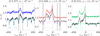 |
Fig. B.1 Photospheric subtraction procedure for the [O I] 5577, [O I] 6300, and [S II] 6731 lines in the ES 22.5 spectrum of RU Lup. The black lines are the observed spectra. The colored lines superposed on the observed spectra are from the K7 template for the photospheric spectrum of RU Lup, veiled to match the depth of the photospheric lines. Above these spectra are the photospheric-subtracted spectra, shifted vertically by 0.2 for clarity. The shaded areas mark the region where the photospheric spectrum is not completely removed. |
Appendix E Synthetic absorption profiles from a rotating and outflowing ring
In this Appendix we highlight the details of the model used to interpret the discrete absorption components in terms of a rotating and outflowing structure. We considered a cylindrical coordinate system (r, ϕ, z), where r represents the distance from the rotation axis in the x-y plane, ϕ is the azimuthal angle measured relative to the x-axis, and z corresponds to the rotation axis (Fig. E.1). In cylindrical coordinates the velocity vector is  . The unit vectors are given by
  in Cartesian coordinates. The radial velocity is vrad = −υ · ŝ, where ŝ = (sin i⋆, 0, cos i⋆) represents the observer’s line of sight. The dot product yields
 (E.1)
(E.1)
Assuming that the poloidal flow is predominantly parallel to the z-axis, we can neglect vr with respect to vz. Then, the shape of the line profile depends on the angles ϕ1 and ϕ2 which limit the sampled region in azimuth.
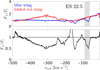 |
Fig. D.1 Extraction of the LVA component of the Na I D2 line in the ES 22.5 spectrum. The top panel shows the red wing line folded onto the blue wing. The bottom panel shows the ratio between the blue wing and the red wing, from which we computed the optical depth and EW. The shaded area marks the velocity extension of the LVA, as defined in Fig. 3. |
To compute the absorption profiles produced by the ring, we generated an array of azimuth angles (ϕ) between ϕ1 and ϕ2, and calculated the local optical depth as
![Mathematical equation: $d{\tau _v}\left( \phi \right) = {\tau _0}{1 \over {\sqrt {2\pi } \sigma }}{\rm{exp}}\left[ { - {{{{\left( {v - {v_{{\rm{rad}}}}\left( \phi \right)} \right)}^2}} \over {2{\sigma ^2}}}} \right]. $](/articles/aa/full_html/2025/12/aa54624-25/aa54624-25-eq52.png) (E.2)
where vrad(ϕ) and σ represent the center and standard deviation of the Gaussian function, and τ0 is a scaling parameter. Using the radial velocity law of Eq. (E.1), we summed all contributions in ϕ to produce the total optical depth τv as a function of velocity. Then, we computed the resulting normalized line profile as
(E.2)
where vrad(ϕ) and σ represent the center and standard deviation of the Gaussian function, and τ0 is a scaling parameter. Using the radial velocity law of Eq. (E.1), we summed all contributions in ϕ to produce the total optical depth τv as a function of velocity. Then, we computed the resulting normalized line profile as
![Mathematical equation: ${F_v} = 1 - {\rm{CF}}\left[ {1 - {\rm{exp}}\left( { - {\tau _{\rm{v}}}} \right)} \right],$](/articles/aa/full_html/2025/12/aa54624-25/aa54624-25-eq53.png) (E.3)
where CF is the covering factor, that is, the fraction of the emission region that is covered.
(E.3)
where CF is the covering factor, that is, the fraction of the emission region that is covered.
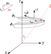 |
Fig. E.1 Sketch of the geometry of the rotating and outflowing sector of a ring in cylindrical coordinates. |
The shape of the line profile depends on the velocities vz and vϕ, the angles ϕ1 and ϕ2, and the scaling parameters σ, τ0, and CF. Figure E.2 displays examples of absorption profiles produced with this model for typical velocities observed in the LVA, that is, vz = 70 km s−1 and vϕ = 50 km s−1. We assumed that the local broadening is thermal, that is, σ = (2kBT/AmH)1/2, where kB is the Boltzmann constant, T is the temperature, mH is the hydrogen mass, and A is the atomic number. In Fig. E.2, we fixed T = 1000 K and A = 11 (sodium), which yielded σ = 1.22 km s−1.
The profiles have two main characteristics. First, they are double-dipped and the velocities of the dips are v1 = −vz cos i⋆ + vϕ sin ϕ1 sin i⋆ and v2 = −vz cos i⋆ + vϕ sin ϕ2 sin i⋆. Second, when the profiles are symmetric, the center is at v0 = −vz cos i⋆.
Appendix F Inferring the outflow properties from the ring fit
Our fit of the double-dipped absorption components (Sect. 4.3) disentangles vϕ from vz. From these values, we developed a procedure to infer the launching radius r0 and the magnetic lever arm λ of the outflow under the assumption of a steady, axisymmetric, cold magneto-centrifugal wind (Ferreira et al. 2006).
F.1 Geometrical estimate of the absorbing radius
Although we do not directly know rabs, the absorbing parcel of gas must lie at the intersection between a streamline and the line of sight (LOS) to the line-emitting region. The streamline can be parameterized as a straight line that originates from the disk at cylindrical radius r0 and has an inclination θs (measured from the disk normal), i.e., z = (r − r0)/ tan θs. The line emission is assumed to come from the blueshifted portion of the magnetosphere, located at cylindrical radii rmag ∈ [0, RT], where RT is the disk truncation radius. Therefore, the LOS has the expression z = (r +rmag)/ tan i⋆. By solving for the intersection between these two lines, we find
 (F.1)
(F.1)
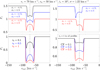 |
Fig. E.2 Gallery of absorption profiles from a vertically-narrow region of a wind which is extended in azimuth. In all plots, vz = 70 km s−1, vϕ = 50 km s−1, i⋆ = 16°, and σ = 1.22 km s−1. If not reported, the parameters are ϕ1 = −π/2, ϕ2 = π/2, τ0 = 0.1, and CF = 1. The vertical dashed lines are at −vz cos i⋆. |
The only physical solutions are the ones in which absorption takes place above the disk plane (z > 0). This condition implies that the streamline must be less inclined than the line of sight, that is, θs < i⋆. A schematic view of the adopted geometry is shown in Fig. F.1.
For the following, we define the geometry factors
 (F.2)
so that rabs = K r0 + α rmag.
(F.2)
so that rabs = K r0 + α rmag.
F.2 Solving for the launching radius
Combining the geometrical constraint of rabs with the cold disk wind relations gives three equations for the three unknowns r0, λ, and rabs, that is,
 (F.3)
(F.3)
Substituting λ and rabs (first and second equation of the system, respectively) into the third equation, and dividing by  , we obtain Eq. (6) for
  . The positive real roots of this equation give r0 = y2.
F.3 Launching properties of the outflow
To explore the properties of the winds traced by the LVA and MVA, we solved Eq. (6) and plotted the resulting curves of r0 as a function of rmag for a grid of θs values at fixed i⋆ = 16°. Figure F.2 shows the LVA in ES 22.5, while Figs. F.3 and F.4 display the MVA in ES 22.3 and ES 22.4, respectively.
The parameter space is restricted by physically motivated bounds on r0. We impose a lower bound at the stellar surface, r0 > R⋆, and an upper bound set by the maximum distance L at which the absorption components can form. In cylindrical geometry rabs = L sin i⋆, and Eq. (F.1) then yields an upper limit on r0 as a function of rmag. Based on the results in Sect. 4.2, we adopt a conservative value of L = 1 AU, that is, rabs ≲ 0.276 AU ≃ 26.2 R⋆.
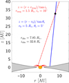 |
Fig. F.1 Example of the geometrical model used to estimate the absorbing radius of the discrete absorption components. The red dashed line represents the line of sight to the magnetosphere. The blue line shows a streamline launched from the disk. The black dot marks the intersection point between the two lines, which defines the location of the absorbing gas. |
Several trends emerge from the figures. As θs → i⋆, the solutions diverge to non-physical r0. For fixed θs they also rise rapidly with increasing rmag. The strongest constraint comes from the limit on rabs: for both components we obtain r0 ≲ 6.76 R⋆. Although θs is formally limited only by θs < i⋆, in practice it is confined to a narrow interval. For rmag ≲ 2 R⋆, one requires θs ≳ 12° to satisfy the lower bound on r0, and θs ≲ 14° to remain below the upper bound.
Despite similar vz, the differing vϕ for the MVA in ES 22.3 and ES 22.4 shift the curves with same θs into different regions of the parameter space. For example, while for the MVA in ES 22.3 the solution with θs = 12.4° has rmag ≲ 1 R⋆, the same solution has rmag ≳ 2 R⋆ for the MVA in ES 22.4. Assuming that the absorption is formed against the magnetospheric line emission and the stellar continuum (i.e., rmag ≲ 2R⋆), this implies a increase of ∆θs ∼ 1-1.5° in the inclination of the streamlines between ES 22.3 and ES 22.4.
Given its lower vz, the LVA requires a smaller magnetic lever arm than the MVA at a given r0. We find λLVA ∈ [1.56, 1.93] and λMVA ∈ [1.75, 3.20].
Appendix G Partial coverage of continuum and line emission
In this Appendix we show how partial coverage of the Ca II line–emitting region can hide absorption at LVA velocities while allowing the MVA to appear strong and remain above the continuum. We define:
C as the Ca II continuum flux,
L(v) as the intrinsic Ca II line emission profile,
τ as the optical depth of the absorber,
CFc as the covering fraction of the continuum source,
CFℓ as the covering fraction of the line-emitting region,
F(v) as the observed flux including absorption.
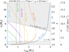 |
Fig. F.2 r0 vs. rmag plot for the LVA in ES 22.5. Colors denote different θs. Solid, dashed, and dotted curves indicate distinct solution branches of Eq. (6). The black dash–dotted lines mark the lower (stellar radius R⋆) and upper (given by the maximum distance at which absorption can form) limits on r0. The shaded areas indicate the excluded regions. The axes on the right show the corresponding magnetic lever arm λ and specific angular momentum ℓ, computed using vz, r0 and Eqs. (3) and (4). |
With independent partial covering of continuum and line emission, the full profile is
![Mathematical equation: $\displaylines{F\left( v \right) = C\left[ {\left( {1 - {\rm{C}}{{\rm{F}}_c}} \right) + {\rm{C}}{{\rm{F}}_c}{e^{ - \tau }}} \right] \cr \; + L\left( v \right)\left[ {\left( {1 - {\rm{C}}{{\rm{F}}_\ell }} \right) + {\rm{C}}{{\rm{F}}_\ell }{e^{ - \tau }}} \right]. \cr} $](/articles/aa/full_html/2025/12/aa54624-25/aa54624-25-eq59.png) (G.1)
(G.1)
The underlying emission profile at velocity v is C + L(v). The fractional absorption relative to this level is
 (G.2)
(G.2)
The ES 22.5 spectrum has S/N = 46, and we adopt a 3σ visibility threshold, meaning that absorption is undetected if the fraction of Eq. (G.2) is smaller than  . This way, we get a threshold for the overlap of the absorbing region with the line emitter, that is,
![Mathematical equation: ${\rm{C}}{{\rm{F}}_\ell } < {{\varepsilon \left[ {1 + L\left( v \right)/C} \right] - {\rm{C}}{{\rm{F}}_{\rm{c}}}\left( {1 - {{\rm{e}}^{ - \tau }}} \right)} \over {\left( {L\left( v \right)/C} \right)\left( {1 - {e^{ - \tau }}} \right)}}.$](/articles/aa/full_html/2025/12/aa54624-25/aa54624-25-eq62.png) (G.3)
(G.3)
Figure 3 indicates that at the LVA velocities the Ca II K emission is very bright, with L/C ≈ 30. Under the assumption that the LVA gas crosses the stellar continuum but misses the line emitter, we set CFc ≃ 1 and solve Eq. (G.3) for CFℓ. The result is
![Mathematical equation: $\displaylines{{\rm{C}}{{\rm{F}}_\ell } < {{\varepsilon \left( {1 + {\rm{L}}/{\rm{C}}} \right)} \over {\left( {{\rm{L}}/{\rm{C}}} \right)\left( {1 - {{\rm{e}}^{ - \tau }}} \right)}} - {1 \over {{\rm{\;L}}/{\rm{C}}}} \cr \;\mathop = \limits^{L/C = 30} {{0.065 \times 31} \over {30\left[ {1 - {e^{ - \tau }}} \right]}} - {1 \over {30}}. \cr} $](/articles/aa/full_html/2025/12/aa54624-25/aa54624-25-eq63.png) (G.4)
(G.4)
For representative Ca II opacities at the LVA velocity of τ = 0.5, 1, and 2, we find CFℓ ≲ 0.14, 0.07, and 0.05. Thus, with L/C ≈ 30 the LVA remains undetected in Ca II as long as it is projected against the line emitter with CFℓ ∼ 10%, even though it fully covers the continuum (CFc ≈ 1).
For the MVA, Fig. 3 shows that the absorption is deep relative to the line but the profile never falls below the continuum. This suggests that the absorbing gas fully covers the line-emitting region (CFℓ ≈ 1) but is weakly projected against the continuum source (CFc ≪ 1), so that F(v)/C ≈ 1 + (L(v)/C)e−τ and the absorbed flux remains above the continuum (i.e., F(v)/C > 1). In summary, this analysis suggests that the visibility contrast between LVA and MVA in Ca II is governed primarily by geometry and not by large differences in ionization.
All Tables
All Figures
|
Fig. 1 Photosphere-subtracted profiles of the [O I] 5577, [O I] 6300, and [S II] 6731 lines in the ES 22.5 spectrum of RU Lup, and best-fitting combinations of Gaussian functions. |
| In the text | |
|
Fig. 2 Profiles of the Ca II H & K and Na I D2 & D1 doublets in the ES 22.5 spectrum of RU Lup. The Ca II H & K lines are plotted in velocity relative to their rest wavelengths. The Na I doublet is plotted in velocity relative to the rest wavelength of the D2 line. |
| In the text | |
|
Fig. 3 Discrete absorption components observed for the Na I D2 (green) and Ca II K (blue) lines in the ES 22.5 spectrum of RU Lup. The shaded areas mark the velocity ranges where absorption is observed. |
| In the text | |
|
Fig. 4 Variability of the Ca II K and Na I D2 lines in the high resolution ESPRESSO spectra (Table A.1). The shaded areas mark the velocity ranges where absorption is observed. These ranges are the same as in Fig. 3 for the spectra from 2022, while the velocity range of the MVA is different in 2021, being [−150, −110] km s−1. |
| In the text | |
|
Fig. 5 Comparison of the Ca II K (blue) and [S II] 6731 (magenta) lines for a selection of RU Lup spectra. From top to bottom, the spectra are from UVES, ESPaDOnS, and ESPRESSO. The Ca II K lines were scaled by a factor of 1/40. The shaded areas trace the evolution of the two components, while the vertical lines mark the peak vrad of the HVC. |
| In the text | |
|
Fig. 6 Best-fit (red line) to the normalized absorption profile of the LVA component in the Na I D2 line from the ES 22.5 spectrum (black line). The profile is the same as that of Fig. D.1. Regions excluded from the fit are plotted in gray. |
| In the text | |
|
Fig. 7 Same as Fig. 6, but for the MVA component in the Na I D1 line from the ES 22.3 and ES 22.4 spectra. |
| In the text | |
|
Fig. 8 Neutral fraction of sodium (χ) as a function of T, computed using the Saha equation for different values of ne. The dash-dotted line marks the critical neutral fraction χb required for the MVA wind torque to balance the accretion torque (see Sect. 5.5). |
| In the text | |
|
Fig. 9 Sketch of the outflow structure of RU Lup inferred from our analysis. The figure is not to scale. |
| In the text | |
|
Fig. B.1 Photospheric subtraction procedure for the [O I] 5577, [O I] 6300, and [S II] 6731 lines in the ES 22.5 spectrum of RU Lup. The black lines are the observed spectra. The colored lines superposed on the observed spectra are from the K7 template for the photospheric spectrum of RU Lup, veiled to match the depth of the photospheric lines. Above these spectra are the photospheric-subtracted spectra, shifted vertically by 0.2 for clarity. The shaded areas mark the region where the photospheric spectrum is not completely removed. |
| In the text | |
|
Fig. D.1 Extraction of the LVA component of the Na I D2 line in the ES 22.5 spectrum. The top panel shows the red wing line folded onto the blue wing. The bottom panel shows the ratio between the blue wing and the red wing, from which we computed the optical depth and EW. The shaded area marks the velocity extension of the LVA, as defined in Fig. 3. |
| In the text | |
|
Fig. E.1 Sketch of the geometry of the rotating and outflowing sector of a ring in cylindrical coordinates. |
| In the text | |
|
Fig. E.2 Gallery of absorption profiles from a vertically-narrow region of a wind which is extended in azimuth. In all plots, vz = 70 km s−1, vϕ = 50 km s−1, i⋆ = 16°, and σ = 1.22 km s−1. If not reported, the parameters are ϕ1 = −π/2, ϕ2 = π/2, τ0 = 0.1, and CF = 1. The vertical dashed lines are at −vz cos i⋆. |
| In the text | |
|
Fig. F.1 Example of the geometrical model used to estimate the absorbing radius of the discrete absorption components. The red dashed line represents the line of sight to the magnetosphere. The blue line shows a streamline launched from the disk. The black dot marks the intersection point between the two lines, which defines the location of the absorbing gas. |
| In the text | |
|
Fig. F.2 r0 vs. rmag plot for the LVA in ES 22.5. Colors denote different θs. Solid, dashed, and dotted curves indicate distinct solution branches of Eq. (6). The black dash–dotted lines mark the lower (stellar radius R⋆) and upper (given by the maximum distance at which absorption can form) limits on r0. The shaded areas indicate the excluded regions. The axes on the right show the corresponding magnetic lever arm λ and specific angular momentum ℓ, computed using vz, r0 and Eqs. (3) and (4). |
| In the text | |
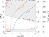 |
Fig. F.3 Same as Fig. F.2, but for the MVA in ES 22.3. |
| In the text | |
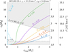 |
Fig. F.4 Same as Fig. F.2, but for the MVA in ES 22.4. |
| In the text | |
Current usage metrics show cumulative count of Article Views (full-text article views including HTML views, PDF and ePub downloads, according to the available data) and Abstracts Views on Vision4Press platform.
Data correspond to usage on the plateform after 2015. The current usage metrics is available 48-96 hours after online publication and is updated daily on week days.
Initial download of the metrics may take a while.