| Issue |
A&A
Volume 704, December 2025
|
|
|---|---|---|
| Article Number | A185 | |
| Number of page(s) | 17 | |
| Section | Extragalactic astronomy | |
| DOI | https://doi.org/10.1051/0004-6361/202554805 | |
| Published online | 12 December 2025 | |
Die Hard: The on-off cycle of galaxies on the star formation main sequence
1
Excellence Cluster ORIGINS, Boltzmannstr. 2, 85748 Garching bei München, Germany
2
Universitäts-Sternwarte, Fakultät für Physik, Ludwig-Maximilians-Universität München, Scheinerstr. 1, 81679 München, Germany
3
Max-Planck-Institut für Astrophysik, Karl-Schwarzschild-Str. 1, 85748 Garching, Germany
4
Max-Planck-Institute for Extraterrestrial Physics, Giessenbacherstr. 1, 85748 Garching, Germany
★ Corresponding author: This email address is being protected from spambots. You need JavaScript enabled to view it.
Received:
27
March
2025
Accepted:
26
September
2025
Abstract
Context. Our picture of galaxy evolution currently assumes that galaxies spend their life on the star formation main sequence (SFMS) until they are eventually quenched. However, recent observations show indications that the full picture might be more complicated.
Aims. We reveal typical in-situ star formation histories and their relations to large-scale environment as well as gas accretion across cosmic time. We further discuss systematic imprints on stellar masses, ages, and metallicities.
Methods. We follow the evolution of central galaxies in the highest-resolution box of the MAGNETICUM PATHFINDER cosmological hydrodynamical simulations and classify their evolution scenarios with respect to the SFMS.
Results. We find that a major fraction of the galaxies undergoes long-term cycles of quenching and rejuvenation on gigayear timescales. This expands the framework of galaxy evolution from a secular evolution to a sequence of multiple active and passive phases. Only 14% of field galaxies on the SFMS at z ≈ 0 actually evolved along the scaling relation, while the bulk of star-forming galaxies in the local Universe have undergone cycles of quenching and rejuvenation. In this work we describe the statistics of these galaxy evolution modes and how this impacts their mean stellar masses, ages, and metallicities today. We further explore possible explanations and find that the geometry of gas accretion at the halo outskirts shows a strong correlation with the star formation rate evolution, while the density parameter as a tracer of environment shows no significant correlation. A derivation of star formation rates from gas accretion with simple assumptions only works reasonably well in the high-redshift universe, where accreted gas is quickly converted into stars.
Conclusions. We conclude that an evolution scenario consistently on the main sequence is the exception, when regarding galaxies on the main sequence at lower redshifts. Galaxies with rejuvenation cycles can be distinguished well from main-sequence-evolved galaxies, both in their halo accretion modes and in their features at z ≈ 0.
Key words: methods: numerical / galaxies: evolution / galaxies: formation / galaxies: general / galaxies: star formation
© The Authors 2025
 Open Access article, published by EDP Sciences, under the terms of the Creative Commons Attribution License (https://creativecommons.org/licenses/by/4.0), which permits unrestricted use, distribution, and reproduction in any medium, provided the original work is properly cited.
This article is published in open access under the Subscribe to Open model. This email address is being protected from spambots. You need JavaScript enabled to view it. to support open access publication.
1. Introduction
The transformation of diffuse gas into stars is a process that spans from large-scale structure formation (e.g., van de Weygaert & Bond 2008) down to giant molecular clouds (GMCs) that host star-forming clumps (e.g., McKee & Ostriker 2007). As baryonic physics is subject to a chaotic interplay of gravitation and hydrodynamics with cooling, heating, and dust formation as well as feedback from stars, supernovae, and active galactic nuclei (AGN), it is remarkable that structure and star formation in galaxies produces characteristic relations and evolutionary pathways. In a color-magnitude diagram, active galaxies form a “blue cloud” separated from the “red sequence” (e.g., Strateva et al. 2001; Balogh et al. 2004) with fewer galaxies occupying the “green valley” in between (Wyder et al. 2007). Additionally, active galaxies are observed to follow a relation between their stellar masses and star formation rates (SFRs), which is called the “star formation main sequence” (SFMS) (e.g., Speagle et al. 2014; Pearson et al. 2018; Leslie et al. 2020; Popesso et al. 2023). Consistent findings of a declining SFMS toward lower redshifts show that the cosmological conditions for conversion of gas into stars change with redshift (e.g., Teklu et al. 2023). This can also be seen from studies of the star formation rate density (SFRD), which evolves with a universal peak at z ≈ 2 and a lower total SFRD at both higher and lower redshifts (Madau & Dickinson 2014). These results for the SFRD evolution are consistent with a general decline of specific star formation rates (sSFR = SFR/M*) in galaxies at later times, which corresponds with a decline of the overall SFMS. However, the different mass- and redshift-dependent descriptions of the main sequence (e.g., Pearson et al. 2018; Santini et al. 2017; Speagle et al. 2014) show that the physics behind the scaling relation are not yet fully understood.
Lin et al. (2024) used Atacama Large Millimeter/submillimeter Array (ALMA) observations and galaxies from the Mapping Nearby Galaxies at APO (MaNGA) survey and found “green valley” galaxies that displayed low SFRs despite having similar amounts of dense gas as main-sequence galaxies. Even with constant and smooth accretion, internal processes of a galaxy are expected to lead to a scatter of ΔMS = log(SFR/SFRMS)≈0.3 dex around the main sequence at different redshifts (e.g., Noeske et al. 2007; Whitaker et al. 2012; Speagle et al. 2014; Pearson et al. 2018). Tacchella et al. (2016) tested the scatter at z > 1 using results from the VELA zoom-in simulation suite, and they attribute this to a cycle of compaction, depletion, and accretion in galaxies until gas inflow from the cosmic web comes to an end. Mergers provide an additional mode of increased star formation activity, either as a consequence of a wet merger-induced starburst or through enhanced gas compaction via interaction with a galaxy (Gómez-Guijarro et al. 2022). In our current picture of galaxy formation, it is usually assumed that galaxies evolve along the main sequence until they are quenched by one of the commonly discussed processes, such as galaxy mergers (e.g., Kormendy & Ho 2013; Ellison et al. 2022) or halo mass quenching (Birnboim & Dekel 2003; Dekel & Birnboim 2008). However, cases of rejuvenation have been discussed lately, as evidence of this has been seen not only at high redshifts (Remus & Kimmig 2025; Trussler et al. 2025) but also at low redshifts (e.g., Yi et al. 2005; Chauke et al. 2019). Recently, models also predict that rejuvenation might be a common occurrence in galaxy formation (e.g., Zhang et al. 2023; Tanaka et al. 2024). However, as of yet it is unclear how common this process really is and how often a galaxy simply evolves along the main sequence, as is commonly assumed.
The principle of mass conservation in its application as the “bathtub” gas regulator model for smooth accretion (e.g., Bouché et al. 2010; Lilly et al. 2013; Burkert 2017) provides a simple framework to test our understanding of the interplay of gas flows and star formation. This interplay is governed by the depletion time tdepl ≡ Mgas/SFR ∼ 1 Gyr (Tacconi et al. 2020), where processes such as the recycling of gas in a “halo fountain” (Oppenheimer & Davé 2008; Tumlinson et al. 2017) and cooling become important. In order to identify typical star formation histories (SFHs) and quantify their prevalence, we studied and classified long-term trends of galaxies in the MAGNETICUM PATHFINDER cosmological simulations1. This paper is structured as follows: In Section 2, we describe the simulation used for this work. Then, we describe in Section 3 the method employed to identify moments of quenching and rejuvenation as well as how we use them to classify the formation histories of the galaxies in our sample. We then show how these classes differ at z ≈ 0 with respect to their mean ages, metallicities, and mass distributions in Section 4. Finally, we investigate the causes of the different characteristic formation classes by measuring gas flow rates, gas flow geometries, and the environment in Sections 5 and 6.
2. The MAGNETICUM simulations
We perform our analysis using Box4 uhr of the MAGNETICUM PATHFINDER cosmological hydrodynamical simulation suite (Teklu et al. 2015). These simulations are based on the cosmological parameters from the WMAP7 results according to Komatsu et al. (2011) with a mass density of Ωm = 0.272, a baryon fraction of fbaryon = 0.168, a cosmological constant of Λ = 0.728 and a dimensionless Hubble constant of h = 0.704. The simulations were run with a modified version of the smoothed-particle hydrodynamics (SPH) code GADGET-2 (Springel et al. 2001a; Springel 2005) with updates regarding the SPH kernel and treatment of viscosity (Dolag et al. 2005; Beck et al. 2016; Donnert et al. 2013).
The baryonic physics includes gas cooling, star formation, and stellar winds as described by Springel & Hernquist (2003). Accordingly, gas particles include contributions to the hot and cold phases with star formation based on the latter. Exchange between the two phases is implemented through radiative cooling on one hand with rates based on cooling tables from Wiersma et al. (2009). Their results are based on calculations using the code CLOUDY (Ferland et al. 1998) while considering contributions from the eleven elements H, He, C, N, O, Ne, Mg, Si, S, Ca, and Fe, which are traced individually within the simulation for all stellar and gas particles, with exposition to the cosmic microwave background radiation and the UV/X-ray background radiation from galaxies and quasars according to the model by Haardt & Madau (2001).
Star formation, supernovae (SNe), and chemical enrichment are implemented as a subresolution model according to Tornatore et al. (2003, 2007), Dolag et al. (2017) with initial stellar population distribution according to Chabrier (2003). The SN feedback is implemented partly as heating and partly as galactic winds with vwind = 350 km/s triggered from a 10%-fraction of SNe II (1051 erg). Black hole growth and AGN feedback are modeled as described by Springel et al. (2005), Di Matteo et al. (2005) with modifications covered by Fabjan et al. (2010) and Hirschmann et al. (2014). AGN luminosities are derived from the BH accretion rate as  , with a radiative efficiency of ϵr = 0.1 for a non-rapidly spinning black hole (Shakura & Sunyaev 1973). Of the total radiated energy, ϵf = 10% is thermally coupled to the surrounding gas, leading to a feedback energy rate of
  . Thermal conduction in galaxy clusters is implemented as described by Dolag et al. (2004) but with a value of 1/20 (instead of 1/3) of the Spitzer value (Spitzer 1962), since anisotropic conduction effects create a net heat transport corresponding to a Spitzer value of one percent, while values of more than ten percent lead to oversmoothed temperature profiles, as shown by Arth et al. (2014).
With a box size of 48 h−1 Mpc, the simulation volume contains 1318 central galaxies with a final z = 0 stellar mass of M* ≥ 1 × 10¹⁰ M⊙. These central galaxies are the SUBFIND-identified dominant galaxies of each halo lying at the center of the potential well, thus excluding satellites. For the given box size, our sample represents primarily field galaxies, with only a few group and cluster centrals. We choose central galaxies with this stellar mass threshold in order to reliably trace galaxies, including their kinematics, with a sufficient particle resolution of N* > 5000. This is a consequence of the resolution given by particles masses of mdm = 3.6 × 10⁷ h−1 M⊙ and mgas = 7.3 × 10⁶ h−1 M⊙ and softening lengths of  and ϵ* = 0.7 h−1 kpc. Each gas particle can spawn a star particle up to four times resulting in lower masses for stellar particles of m* ≈ 1.8 ⋅ 106 h−1 M⊙. Gas particles are not fully consumed upon forming a star particle but instead are capable of spawning up to four star particles, which is a unique advantage of the MAGNETICUM PATHFINDER simulations. Not only does this increase the stellar mass resolution by a factor of four, but it also better accounts for the more typical process of GMCs to partially outlive star formation and absorb momentum and chemical enrichment from stellar feedback (e.g., Chevance et al. 2023). Specifically, a gas particle can form stars at its current metallicity, then be further enriched and ejected by the stellar feedback and potentially return to resume star formation later.
The simulation has been shown to reproduce several critical galaxy properties in previous works, for example with respect to scaling relations across different redshifts (e.g., Teklu et al. 2015, 2017; Remus & Forbes 2022; Dolag et al. 2025), the kinematical properties of galaxies (e.g., Schulze et al. 2018; van de Sande et al. 2019; Valenzuela et al. 2024), and the star formation properties of galaxies (e.g., Kudritzki et al. 2021; Teklu et al. 2023). It is especially noteworthy that the galactic scaling relations arise naturally while the tuning of the MAGNETICUM PATHFINDER simulations was toward hot halos of galaxy clusters. Furthermore, the simulation suite captures galaxy properties at the higher redshifts of z ≈ 4, which is of particular difficulty (e.g., Lustig et al. 2023; Remus & Kimmig 2025; Kimmig et al. 2025; Dolag et al. 2025), but especially relevant in the context of this study where we trace galaxy properties through cosmic time.
We traced a set of galaxies by following the most massive progenitors along halo merger trees of SUBFIND-identified galaxies with a baryonic adaptation by Dolag et al. (2009) of the work by Springel et al. (2001b). To clean the sample from rare cases of broken merger trees, we disregard galaxies with an abrupt termination of their merger tree at z < 1, since this makes it difficult to compare with galaxies that are traced back to cosmic noon and beyond. Additionally, we remove galaxies that do not enter the SFMS before z > 1, reducing out final sample from 1318 to 1282 galaxies, which we plot in Figure 1.
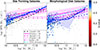 |
Fig. 1. Star formation main sequence at z ≈ 0. The left- and right-hand panels show the results with respect to two selection criteria for MAGNETICUM galaxies. By imposing a threshold of sSFR > 0.2/tHub (left), as used by Carnall et al. (2020) (dashed black line), we find a slightly higher linear fit to the logarithmic values (dashed blue line) compared to selecting for all kinematic disks with SFR > 0 M⊙/yr (right). Results from observations are displayed in magenta, simulations are shown in blue colors. The solid blue line and shaded region show the running median and 50th percentile region. The circles represent the galaxies from the MAGNETICUM PATHFINDER simulations colored according to their morphology as defined by the b-value (Teklu et al. 2015). Gray circles are ignored for the running median lines on each panel. The SFR values below the range of the figure are fixed to the bottom to represent the full sample in this work. The magenta solid line and shaded region highlights a range of ±0.5 dex around the main sequence fit by Pearson et al. (2018), which we used in this work to distinguish between being on and off the main sequence. The other magenta lines are additional observational results: dashed line (Speagle et al. 2014), dash-dotted line (Leslie et al. 2020), and dotted line (Popesso et al. 2023). The dashed cyan line marks the results from ILLUSTRISTNG by Donnari et al. (2019a). |
Table 1 in Section 3.1 shows that the latter criterion of a period of star formation on the main sequence impacts the total number of galaxies considered. This is especially evident when comparing the total number of galaxies classified with respect to the main sequence by Speagle et al. (2014), for which only 1014 galaxies are among the formation classes discussed in this work.
Number of galaxies within each formation class with respect to expectations according to a list of results for the SFMS.
3. The main sequence and star formation history classes
The relation of galaxy stellar mass and star formation rate has long been known to establish a fundamental difference between two groups of galaxies, with those galaxies that are star-forming living on a relatively tight star formation main sequence, and those that have quenched their star formation lying within a more diffuse cloud below (e.g., Speagle et al. 2014; Pearson et al. 2018; Popesso et al. 2023; Leslie et al. 2020; Brinchmann et al. 2004). This main sequence of galaxies evolves with time, reaching higher SFRs at a given stellar mass at higher redshifts than at lower redshifts, demonstrating an overall decline in star formation to lower redshifts (e.g., Speagle et al. 2014; Pearson et al. 2018). While this global picture is well established, the observed main sequence relations strongly differ between different surveys already at z = 0, as can be seen from Fig. 1, where the different observed relations are shown as pink lines.
We start by testing whether the simulation can reproduce the observed main sequences. Fig. 1 shows in both panels the SFMS found for the MAGNETICUM simulations, in comparison to the results reported from different observations and the IllustrisTNG simulations (Donnari et al. 2019b, dashed cyan line). The left panel shows all galaxies colored according to their morphology as traced by the b-value (Teklu et al. 2015), with blue colors indicating disk galaxies and red colors indicating spheroidals. Yellow colors represent intermediate galaxies. The main sequence from the simulations here is calculated from all galaxies that have sSFRs larger than sSFR > 0.2/tHub, the threshold criterion defined by Carnall et al. (2020), while galaxies below this threshold are plotted in gray. This criterion is similar to that by Franx et al. (2008) commonly used in the literature to split quiescent from star-forming galaxies and included in the figure as black dashed line. The resulting main sequence from MAGNETICUM using this definition is marked as a blue solid line, with the 50th percentile scatter shown as a blue shaded area. The main sequence found for the MAGNETICUM simulations using this definition mirrors the results reported for the IllustrisTNG simulations by Donnari et al. (2019b). It well agrees with the observational relations, though we note the existence of some scatter, such that the observations by Pearson et al. (2018) tend to higher SFRs at lower stellar masses compared to MAGNETICUM, while Leslie et al. (2020) and Popesso et al. (2023) find lower SFRs for the more massive galaxies at z = 0.
The right panel of Fig. 1 shows the main sequence as obtained if only those galaxies that are morphologically classified as disk galaxies are used, with the intermediates and spheroidals plotted in gray. While this criterion does not explicitly select for star-forming galaxies, the absence of blue circles at the bottom of the panel shows that disk galaxies also have higher SFR values. As can be seen immediately, the main sequence obtained from the simulation now is overall at lower values, resembling more the shape of the relation reported by Popesso et al. (2023) or Leslie et al. (2020) before a sudden increase in star formation at  . This is due to the existence of what is commonly referred to as red spirals (e.g., Masters et al. 2010), i.e., galaxies that are morphologically spiral galaxies but their star formation has (partially) been quenched. Their presence demonstrates that the morphology of galaxies is not directly correlated to their star formation properties, even though for the large majority there is the trend of disk galaxies being star-forming. This was already indicated in the left panel of Fig. 1, where the coloring of the data points revealed that several of the galaxies on the main sequence according to their star formation properties are in fact of intermediate morphology (i.e., contain for example large bulges) or even, in a few cases, spheroidals, especially at the higher mass end. Consequently, defining an SFMS is not perfectly straightforward.
3.1. Formation history classification
We want to understand if galaxies live on the main sequence until quenching or not. Thus, we traced galaxies across cosmic time and classify them according to their SFR evolution relative to the SFMS by Pearson et al. (2018). While it is evident from Fig. 1 that the relation found by Pearson et al. (2018) does not fit the best to the Magneticum galaxies, we chose to use their best-fit relation as a reference as they provide a consistent method in obtaining the main sequence covering a large range of redshifts, which is required to study the long-term evolution of galaxies. In addition, their values are based on the same cosmology from WMAP7 results (Komatsu et al. 2011) as well as the IMF by Chabrier (2003). However, we do not limit the study to the relation found by Pearson et al. (2018) but rather explore other main sequence definitions as baseline as well, which we mention throughout this work if differences from the results based on the main sequence by Pearson et al. (2018) are found. Overall, the results presented in this work do not change with the choice of base main sequences, and only the relative fractions of properties vary depending on that choice. An overview of the main sequences used as references and the obtained results is given in Table 1. For each snapshot, we defined the state of each galaxy as follows:
-
Quiescent if it is more than 0.5 dex below the main sequence value SFRMS(M*, z), reaching down to SFR = 0;
-
Star forming if it is within a ±0.5 dex range of the main sequence value; and
-
Star bursting if the SFR is more than 0.5 dex above the main sequence.
Since we looked at long-term trends, we focused on the duration of quiescence instead of intensity. In order to reveal long-term trends, a running median with a window of 1 Gyr is applied first on the SFRs. This smoothed SFR is compared to the SFR of the main sequence to define the galaxy as quiescent, star-forming or star bursting at the given time. This classification is again smoothed over a window of 1 Gyr to identify long-term transitions between quenching and rejuvenation. We require for a change in classification from star-forming to quiescent (or vice-versa) that the galaxy remains with the new state for at least 80% of this period of 1 Gyr.
Following this approach, we found four different characteristic scenarios of evolution, as shown in Figure 2. In the figure, we plot a given galaxy’s sSFR with cosmic time (colored lines) compared to the expected main sequence value for the galaxy’s current stellar mass (black lines and shaded areas), with four representative galaxies for each category (panels going from top to bottom):
-
Main-sequence galaxies (cyan, top panel) maintain a high SFR and never go through periods dominated by quiescence. Only about 2% of the sample never become quenched.
-
Quenched galaxies (dark red, second panel) quench once and never recover an SFR within 0.5 dex of the main sequence. Galaxies that quench permanently make up 65% of the sample.
-
Rejuvenating galaxies (magenta, third panel) quench below the main sequence but recover an SFR according to the main sequence value. Such rejuvenation cycles are found to occur for individual galaxies up to three times in succession. Rejuvenating galaxies form the second-largest class, with ∼32% of the sample.
-
Caught galaxies (blue, bottom panel) are dubbed by virtue of maintaining a constant SFR until the main sequence itself catches it due to its decline with lower redshifts. These formation scenarios were classified manually and only make up ∼2% of the sample.
Few galaxies remain on or above the main sequence throughout their entire evolution and will be referred to as main-sequence-type galaxies. Quenched-type galaxies drop and stay below the main sequence until z ≈ 0. Rejuvenating galaxies hop on and off the main sequence once or multiple times. The caught-type class consists of the galaxies that drop below the main sequence but maintain a constant star formation until they passively get “caught” by the main sequence. This is possible since the main sequence itself decreases with lower redshifts. Seven galaxies surpass their expected SFRs for a main sequence galaxy by 0.5 dex at least 80% within a 1 Gyr time window.
The study was performed using the SFMS fit by Pearson et al. (2018). However, we have reproduced our classifications using also other fits from observations as shown in Table 1, as well as the quiescence limits by Franx et al. (2008), Carnall et al. (2020). While the absolute numbers of galaxies in each class change, a consistent picture emerges, with only a very small fraction of galaxies evolving along the SFMS. The bulk of galaxies quenches at high redshift and a consistently significant fraction of galaxies hops on and off the main sequence, of which also a large part end up on the main sequence at z ≈ 0. As a result, we find that the dominant group of galaxies on the main sequence at z ≈ 0 have experienced passive phases on gigayear timescales, independent of the exact main sequence definition used for classification. Consequently, our classifications of these different star formation behaviors are robust and not simply definition dependent. We do note, however, a systematic difference between the main sequence results depending on wether or not a turnover mass was included in their fit. Those main sequence fits that do (Leslie et al. 2020; Popesso et al. 2023) result in an overall greater number of rejuvenated galaxies (‘R.’ in Table 1) and fewer galaxies that always remained on the main sequence (‘MS.’ in Table 1) as compared to those that do not include a turnover mass (Speagle et al. 2014; Pearson et al. 2018). This is expected due to the redshift evolution of each main sequence description. While the relations by Leslie et al. (2020), Popesso et al. (2023) require higher SFRs at high redshift than the relations by Speagle et al. (2014), Pearson et al. (2018), it is the other way round toward z = 0. In addition, the turnover mass amplifies this effect for more massive galaxies, leading us to the conclusion that rejuvenation is extremely common among galaxies on main sequences with turnover mass.
In Figure 3 we plot the star formation rate versus stellar mass for galaxies of each class (columns, going from left to right as main sequence, quenched, rejuvenator, and caught) from z = 5 down to z = 0.1 (rows, top to bottom). The circle colors in this figure indicate the number of transitions a galaxy has undergone from star-forming to passive. A galaxy that has not yet fallen off the main sequence by the respective redshift is shown in light blue. Galaxies that have quenched once appear as red circles, so a red circle on the main sequence has rejuvenated. Orange colors indicate a second transition into quiescence after rejuvenation and yellow colors indicate a third drop off the SFMS after two rejuvenation cycles. The thin black contour lines show the distribution of our full galaxy sample at each redshift for comparison. We also show the main sequence as defined by Pearson et al. (2018) as a black line (with the shaded area representing ±0.5 dex).
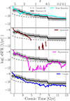 |
Fig. 2. Examples of the four formation scenarios for galaxies with respect to sSFR changes over time. The black lines and shades indicate the main sequence values depending on the redshift and stellar mass of a galaxy according to results by Pearson et al. (2018) with a scatter of ±0.5 dex applied to differentiate between on or off the main sequence. From top to bottom, the panels show a main-sequence-type galaxy (cyan), an early-quenched galaxy (dark red), a rejuvenating galaxy (magenta), and a caught galaxy (blue). Two classes are not explicitly represented here. First, the “late-quenched” types only differ from the “early-quenched” by dropping off the main sequence after redshift z = 1. Second, rejuvenator-main-sequence-type galaxies recover a stable position on the main sequence at redshift z = 0, unlike rejuvenator-quenched-type galaxies, which also go through rejuvenation cycles but do not end up on the main sequence. The vertical lines highlight the snapshots corresponding to each row in Figure 3. |
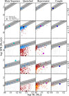 |
Fig. 3. Star formation main sequence evolution of the MAGNETICUM galaxies traced back from the selection made at z = 0 (bottom-row panels). The rows contain snapshots with decreasing redshift from top to bottom between 6 < z < 0. From left to right, the different sub-samples “Main Sequence”, “Quenched”, “Rejuvenator”, and “Caught” are highlighted by colors in front of the total sample in gray in the background. Light blue data points represent galaxies that have not yet dropped below the main sequence; each quenching event is counted and encoded in the changing color of the data points as red (once), orange (twice), and yellow (three times). The large points are the cherry-picked representative galaxies from Figure 2. Quenched representative galaxies are set as half-circles to the bottom of the panels for visibility. The black line and gray shades correspond to the main-sequence found by Pearson et al. (2018). Gray contours outline the distribution of the full galaxy sample for comparison in each panel. |
As noted, we find the main bulk of our galaxies to be either quenched or rejuvenators. The former show a large spread in quenching times, with some falling off the sequence as early as z = 2.3, while others remain on the main sequence all the way down to z = 0.5 before finally quenching. This is true also for the rejuvenators, except that they continue returning back up to the main sequence. We find that most rejuvenator galaxies undergo their first quenching process at 2 > z > 1 just after the cosmic peak of star formation (Behroozi et al. 2013; Madau & Dickinson 2014). In the following, we discuss each of the classes separately in more detail with the main sequence by Pearson et al. (2018) as a reference.
3.2. Main sequence galaxies
Only ∼2% of all galaxies in our sample and 14% of galaxies on the main sequence at z ≈ 0 manage to always maintain a high star formation rate. Explicitly, this means that they remain on the SFMS from the moment of first appearing on it until the end of the simulation. While galaxies in this class might briefly drop below 0.5 dex of the main sequence, they quickly recover within less than 1 Gyr and show no lasting periods of quiescence.
3.3. Quenched galaxies
About 65% of all galaxies in our sample belong to the quiescent group, remaining on the main sequence until a quenching event brings them below by at least 0.5 dex, after which they never recover significant amounts of star formation. Given the difference in quenching times noted in Figure 3, the class of quenching galaxies is sub-divided into galaxies that quench early, i.e., before z = 1 and those that quench late, after z = 1, well after the peak of star formation. We highlight the difference between these two scenarios in the upper panel of Figure 4, where we show the sSFR against cosmic time (as in the style of Figure 2) for two examples of early (red) and late (blue) quenched galaxies. The early-quenched galaxy drops below the main sequence much more abruptly than the late-quenched galaxy. Interestingly, this example galaxy does rekindle star formation but not consistently and high enough to rejuvenate onto the main sequence. By contrast, the late-quenched galaxy shows a smooth decline in sSFR that follows expectations for a growing main sequence galaxy, before finally dropping of at around z ≈ 0.5.
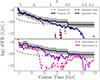 |
Fig. 4. Similar to Figure 2 but focused on the difference between the subclass pairs of early- and late-quenched galaxies as well as quenched and main-sequence rejuvenators. The colored dashed lines represent the cases also shown in Figure 2, while the colored solid lines are the subtypes to differentiate. The gray dashed quiescence criteria (Carnall et al. 2020) and black-shaded SFMS expectations (Pearson et al. 2018) are derived from the stellar masses of the latter. This causes the pink dashed main-sequence-rejuvenator to not lie on the SFMS at z ≈ 0 due to the larger stellar mass (see Figure 5) and therefore lower sSFR. The early-quenched galaxy does recover star formation after quenching but never consistently makes it back onto the main sequence. The late-quenched galaxy also almost makes a passive rejuvenation akin to caught-type galaxies, since the main sequence drops at z < 0.5. However, it is still mostly more than 0.5 dex below the main sequence averaged over a smoothing window of one gigayear, ruling out a rejuvenation scenario. The main-sequence rejuvenator undergoes a more pronounced quenched phase than the quenched rejuvenator. |
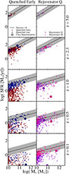 |
Fig. 5. Similar to Figure 3 but focused on the difference between the subclass pairs of early- and late-quenched galaxies as well as quenched and main-sequence rejuvenators. Here, the colors refer to the subclass types instead of quenching incidents. The large points show the cherry-picked representative galaxies from Figure 4, again set to the bottom of the panels as half-circles for visibility in case of low SFR values. By construction, the difference between early- and late-quenched is most pronounced at z = 1. At z ≈ 0, the non-zero distributions are barely noticeable. Analogously, the difference between the two rejuvenator subclasses is the sharpest at z ≈ 0. Both subclasses undergo rejuvenation cycles at different times, but the relation to the SFMS determines the classification. |
More and less rapid quenching scenarios are found among galaxies of both subclasses, as well as small and short-lived rekindling of star formation. To illustrate this distinction further, we plot in the left panel of Figure 5 the SFR against stellar mass of galaxies from the “quenched” class at five different redshifts as in Figure 3, but change the color scheme. Galaxies classified as early quenched are always plotted in red, while late quenchers are always in blue. This allows us to see that the majority of early quenchers still lie on or near the main sequence at z = 2.3, such that their quenching must occur abruptly between 2 > z > 1. Conversely, late quenchers do not surpass the mass range of the figure at z = 2.3 and moment of quenching is less temporally confined, with occurrences spreading evenly between the time steps 1 > z > 0.5 and 0.5 > z > 0. This hints at different causes of quenching between early and late quenching, such as feedback and outflows as opposed to starvation or merger accretion.
The median values of net gas accretion rates relative to dark matter assembly in Figure B.1 in the appendix support the image of an early starburst with a rapid transition toward net outflows for early-quenched galaxies. The relation between black hole mass and stellar mass shown in Figure C.1 in the appendix implies a correlation with AGN feedback, as early-quenched galaxies have the most massive black holes. As shown by Kimmig et al. (2025), an early and rapid formation also comes with an efficient gas transport toward the AGN. In addition to the starburst the feedback by the massive black hole then adds to the complete removal of gas leading to a permanent quenching. Late-quenched galaxies have lower accretion rate peaks and black hole masses, indicating a less rapid evolution due to gas accretion. The prevalence and impact of mergers in the two quenching scenarios will be disentangled in future work.
3.4. Rejuvenating galaxies
Approximately 32% of the galaxies in our sample are rejuvenators, and thus undergo one or more cycles of quenching and rejuvenating back onto the main sequence. As highlighted by the changing colors in the third column of Figure 3, this cycle can repeat up to three times, represented by a red-orange-yellow color scheme for the number of quenching transitions. We find that rejuvenating galaxies rarely quench completely.
The large range of different scenarios producing rejuvenation makes it difficult to find collective similarities in time-sensitive statistics. However, as we discuss in Section 4, this class still reveals collective behavior, suggesting fundamental differences between formation conditions compared to the other classes.
To further study the composition of active galaxies at z ≈ 0, we differentiate rejuvenating galaxies that end up on the main sequence (in this work referred to as “Rejuvenator Main Sequence” or ‘RM’) from those that end up quenched (“Rejuvenator Quenched” or ‘RQ’). The conceptual difference is visualized with the chosen examples in the lower panel of Figure 4, where we plot the sSFR against cosmic time of two example rejuvenator galaxies, one that ends up quenched (RQ, solid lilac line), and one that ends up star-forming (RM, dashed pink line). Even though the quenched rejuvenator has a more consistent SFH, it drops off into a new quenched phase toward z ≈ 0. The main-sequence rejuvenator undergoes an extended period of quiescence until rejuvenating back onto the main sequence in two rejuvenation cycles, ending up as actively star-forming. In the right-hand column of Figure 5, we can see that the two subclasses of rejuvenators are not distinguishable by their location in the SFR versus stellar mass plot at higher redshifts, instead lying alternatively on or off the main sequence. We therefore conclude that there is no physical difference between the two classes of rejuvenators (unlike for the early and late quenchers), with the only distinguishing feature being the timing of their rejuvenation. Intriguingly, we find that rejuvenating galaxies host less massive black holes (see Figure C.1 in the appendix), which may facilitate rejuvenation with less feedback emitted. We note also that the impact of mergers will be studied in future work using merger trees, which connect SUBFIND-identified progenitors of a galaxy through the simulation snapshots. This will allow us to look for differences between galaxy evolution classes regarding the time correlation between merger events and quenching or rejuvenation.
3.5. Caught galaxies
A rare but nonetheless peculiar class of galaxies, namely ∼2% of our sample, consists of such whose SFRs drop below the main sequence at some point but never fully cease their star formation. Instead, they very continuously form stars with a nearly constant rate just below the main sequence, until they reappear on it once the overall main sequence itself has lowered to reach the SFR of these galaxies. An example case of this formation scenario is shown in the bottom panel of Figure 2. We distinguish these galaxies from the rejuvenators, as they never truly rise in their SFR (i.e., rejuvenate), and instead are a result of the overall decline in cosmic SFRD. Members of this galaxy class maintain a constant level of lower SFR, such that caught-type galaxies are especially promising candidates to test the equilibrium prediction of the “bathtub” model (Burkert 2017). Therein, a constant gas accretion rate leads to an equilibrium state between accretion, star formation and feedback, resulting in a constant gas mass and SFR. This formation scenario is particularly interesting since they are technically more stably retaining their star formation compared to the average main sequence galaxy, which is actually lowering its SFR with redshifts. Their small sample size is expected as they continuously contribute to the scatter of the main sequence opposing the definition of a well-constrained SFMS.
4. Imprints of star formation histories
A galaxy’s star formation history depends on their evolutionary history, including both internal and external processes and leaving observable traces in their population of stars at z = 0. Consequently, one could expect to find systematic differences in the galaxy properties of our different evolutionary classes.
To test this, we plot in Figure 6 the median radial profile of the stellar age for all galaxies of a given class, normalized by their stellar half-mass radius. Indeed, we find noticeable differences among our galaxy classes. Quenched galaxies (in the two leftmost panels) display very flat radial age profiles with tage ≈ 10 Gyr, with only a faint trend for late-quenching galaxies toward younger stars in the center. Galaxies that fully evolve along the main sequence have consistently younger stellar populations toward their centers, with the youngest average stellar population in the very center (rightmost panel). Rejuvenating galaxies, especially those that are still on the main sequence at z ≈ 0, produce a “u”-shaped stellar age profile, suggesting that rejuvenation tends to happen outside the stellar half-mass radii, similar to the results reported for high-redshift rejuvenation by Remus & Kimmig (2025). For lower redshifts, Hao et al. (2024) find in MaNGA data a class of blue spirals with signs of rejuvenation, such as a dip in stellar age going from 0.5 to 1.5 ⋅ R1/2 (their profile type three), which is comparable to what we find here. We note that we find a trend of continuously increasing stellar age with radius in the center only for main-sequence-type galaxies. Caught-type galaxies show a similar age distribution as rejuvenating galaxies. This could indicate a degeneracy of radial age profiles with respect to how sudden and steep the transition from below the main sequence to star-forming is.
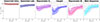 |
Fig. 6. Median radial profiles and 68th percentile spread of stellar ages at z = 0. Before extracting the running median and scatter, we calculated the mean stellar ages for each galaxy in nine equal-width radial bins between 0 and 5 R1/2. The solid lines and shaded regions correspond to the statistics of the class indicated at the top of each panel. The dashed lines are the running medians from the panels to the left of each panel for a direct comparison. Higher values correspond to an older population, which is fairly constant at around ten gigayears for early-quenched galaxies. Main-sequence-type galaxies show increasingly young populations toward the center, while the three types of rejuvenating classes are the youngest at roughly one half-mass radius and increase in age again toward the very center as well as the outskirts. |
Comparing the radial profiles of the different classes suggests an order of transitions, with early star formation starting of with flat profiles, and depending on how strong star formation is retained down to z = 0 the central portion dips down toward younger ages. Quenched early and late have the least such prolonged star formation, with then RQ, then RM, and caught are comparable, and finally those galaxies that are always on the main sequence show the strongest radial age gradient.
Such an order of transitions between the classes also emerges from positions in the age-metallicity diagram of our galaxy sample as we show in Figure 7. For all galaxies, their mean stellar metallicities ⟨Z/H⟩ are shown against their mean stellar ages ⟨tage, *⟩. We find that main-sequence-evolved galaxies represent the extreme end of high metallicities and young ages, while early-quenched galaxies are on the opposite end, strongly concentrated in the low-metallicity-old-age regime, with a significant scatter with respect to metallicity.
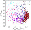 |
Fig. 7. Mean metallicities and ages of the full galaxy sample at z = 0. Less populated classes are in front of larger ones for visibility while slightly decreasing the perceived scatter of the larger classes, such as the early-quenched galaxy class. This class concentrates at high ages and lower metallicities opposing main-sequence types. The intermediate classes of late-quenchers and rejuvenating galaxies bridge the gap in a dichotomous way of age and metallicity combination. |
There emerges then an interesting difference between the late-quenched and rejuvenated-quenched galaxies, with both lying at similar mean stellar ages, but the former having much higher stellar metallicities than the latter. This implies that the stars formed in RQ galaxies were made of significant amounts of pristine gas, drawn from the cosmic web with little chemical enrichment, while late-quenchers continually enriched their gas and thus their newly formed stars, much like main sequence galaxies, before finally quenching. This is also why they lie in the transition between early-quenched and main sequence galaxies.
Curiously, though the RM-type galaxies are the overall youngest, together with the main-sequence galaxies, they tend toward much lower metallicities, comparable to their older RQ counterparts. Thus, it seems that low stellar metallicity in massive galaxies is found for two cases. Either the galaxy formed and quenched rapidly in the early universe or its star formation was not continuous, instead involving cycles of gas ejection, quiescence, and re-accretion of more pristine, metal-poor gas that thus reduced the overall stellar metallicity. Conversely, remaining constantly on the main sequence requires some degree of gas retention and thus leads to the overall highest stellar metallicities.
The turbulent star formation histories with rejuvenation cycles also leave their imprint in the galaxies’ stellar abundance ratios of oxygen to iron [O/Fe] and iron to hydrogen [Fe/H], which are measures of the fast α enrichment via type II supernovae and the slow iron enrichment via type Ia supernovae, respectively. To demonstrate this, Figure 8 shows the mean abundance ratio relation [O/Fe] vs [Fe/H] of each galaxy.
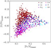 |
Fig. 8. Mean stellar abundance ratios of the galaxy sample at z ≈ 0. Oxygen was chosen to represent α enrichment. Akin to Figure 7, different regions of the diagram are predominantly occupied by specific classes. A clear gradient emerges from the top left to the bottom right of the distribution as QE-QL-RQ-Ct-RM-MS. Main-sequence-type galaxies tend to the right-most corner of the distribution. |
We find that early-quenched galaxies (dark red) populate the highest [O/Fe] values. Then the distribution transitions toward lower [O/Fe] and higher [Fe/H] values via late-quenched (dark blue) and then quenched rejuvenators (lilac). Main-sequence rejuvenators (pink), main-sequence evolved (cyan) and caught-type (blue) classes scatter around the bottom-right edge of the distribution, with rejuvenators at the lowest [O/Fe] values and main-sequence-types with the highest iron values [Fe/H], in agreement with Figure 7 where we find them to boast the highest overall stellar metallicities.
Kimmig et al. (in prep.) show that the chemical evolution of galaxies in the MAGNETICUM PATHFINDER simulations consistently begins at high [O/Fe] and low [Fe/H] values beyond the range of Figure 8, with the initial enrichment dominated by type II supernovae and thus α elements. The stellar metallicities of early-quenched galaxies are frozen in after a period of high star formation, leading to a final state with the highest [O/Fe] values since no additional stars with higher iron enrichment are formed. The slower but steady contribution from type Ia supernovae for galaxies that have more time to evolve drives the distribution toward the lower values of [O/Fe] and higher values of [Fe/H] simultaneously. Interestingly, rejuvenating galaxies display the lowest α enrichment, which supports the picture of pristine gas accretion as the driver of rejuvenation. The detailed treatment considering mass-dependent lifetime functions and metallicity-dependent stellar yields of AGB stars, SNII, and SNIa, produce metallicities consistent with observations (Dolag et al. 2017; Kudritzki et al. 2021; Dolag et al. 2025). Since the dust and gas phases do not segregate on the galactic scale, we expect uncertainties in the IMF and stellar yields models (including for example the binary fraction) to dominate over the impact of dust. Nonetheless, the values shown in this work are to be compared to dust-corrected results.
We show in Figure 9 that producing stars in rejuvenation cycles not only affects the observable combination of age and metallicity, but also correlates with the stellar mass of the galaxy at z = 0. We plot there the fractions of galaxies that belong to each class within a given stellar mass bin.
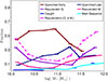 |
Fig. 9. Fractions of formation class members in stellar mass bins at z ≈ 0. Slight shifts of data points originate from taking the median stellar masses instead of bin centers. Early-quenched galaxies (dark red) peak at around M* = 1011, while late-quenched ones (dark blue) peak at slightly higher masses. Galaxies with rejuvenation cycles (dashed magenta line) in their formation histories are more prevalent on the lower- and higher-mass ends of the range between 1010 M⊙ ≤ M* ≤ 1012 M⊙. Quenched rejuvenators (lilac) tend more toward lower masses, while a rejuvenation sustained until z ≈ 0 (pink) is more often found at higher masses. Main-sequence (cyan) and caught types (blue) are generally rare with a faint preference for the high-mass end. Both subtypes are more prevalent on the lower- and higher- mass ends of the range between 1010 M⊙ ≤ M* ≤ 1012 M⊙. |
Interestingly, we find that rejuvenating galaxies (dashed magenta line) lie predominantly at either the low- or high-mass end, which is in part because the overall largest group, the early-quenching galaxies (dark red), concentrates around 1010.5 − 1011 M⊙. By contrast, late-quenching galaxies (dark blue) tend toward slightly higher stellar masses. However, we note that the u-shaped rejuvenator distribution could imply two separate physical mechanisms that dominate. On the right, the increasing rejuvenator fraction with increasing stellar mass may be the result of an increasing number of mergers within their evolutionary history (as the most massive objects have experienced the most mergers), as well as the possibility of cooling from the hot halo (e.g., Fabian & Nulsen 1977; Sarazin 1986; González Villalba et al. 2025). To investigate the cause of the bimodal distribution, splitting the rejuvenators up by their stellar mass into high- and low-mass subclasses should reveal collective differences in gas accretion evolution, in-situ fractions and merger histories. The latter would be a plausible main driver for rejuvenation of the higher-mass galaxies for which smooth accretion is quenched by shock heating by their hot halos (e.g., Dekel & Birnboim 2006). Furthermore, explicitly tracing gas particles would provide further insight into the different mass assembly histories, which is a topic for future work.
For the low-mass end at M* ≈ 1010 M⊙, we find that quenched-early and quenched-late account for 52%, which increases up to 70 − 80% by M* ≈ 1011.25 M⊙. This is because gas falling into halos with a virial mass greater than Mvir ≳ 1012 M⊙ (galaxy stellar masses of M* ≳ 3 × 10¹⁰ M⊙) gets shock-heated to high temperatures where cooling becomes inefficient (e.g., Rees & Ostriker 1977). This leads to the apparent knee in the galaxy luminosity function (Schechter 1976) and stellar mass function (e.g., Bullock & Boylan-Kolchin 2017). Consequently, it is the increase in those groups that leads to the decrease in rejuvenated galaxies.
However, simply becoming quenched does not mean a galaxy may not rejuvenate. Instead, we note that the lower rate of rejuvenated galaxies toward intermediate mass galaxies may be required by construction, as to reach stellar masses of M* > 1010.5 M⊙ requires a high SFR over a long period of time, with simply insufficient time to both quench and rejuvenate. Indeed, the late-quenched galaxies are those that rise the strongest with increasing stellar mass, meaning that they represent galaxies that grew significantly in stellar mass by forming it in-situ, before finally running out of gas (or quenching via a dry merger). Simultaneously, low-mass galaxies are more easily quenched, as they have more shallow potential wells (e.g., Dekel & Silk 1986; Efstathiou 2000) and may therefore be more susceptible to short-term ejection and re-accretion of gas, and galaxies that end at lower masses must have on average spent a longer time with such shallow potential wells compared to more massive galaxies.
Generally, we note that rejuvenated galaxies exist at all stellar masses, while our main-sequence galaxies (cyan), though few in number, show a clear trend toward higher masses at z = 0. This is a direct consequence from the constraint of lying on or near the main sequence at all times. When taking an initial galaxy of M* = 108 M⊙ at z = 4, 3, and 2, assuming a Chabrier IMF (Chabrier 2003) with mass loss following Leitner & Kravtsov (2011) and determining its SFR in time steps of 10 Myr based on the evolving Pearson et al. (2018) main sequence, we determine the expected final z = 0 mass as M* = 6 × 10¹⁰ M⊙, 4 × 10¹⁰ M⊙ and 3 × 10¹⁰ M⊙.
We note that this is assuming an ex situ fraction of 0% such that the true mass is likely higher and that assuming a Kroupa (2001) IMF would only increase the final mass due to the higher fraction of low-mass stars. Consequently, it is essentially by construction that observed lower mass galaxies at z = 0 must have undergone some periods of quiescence or must have formed incredibly late in cosmic time (after the peak of the cosmic SFRD).
Another formation pathway for star-forming galaxies is belonging to the caught-type class, which we only find toward the low-mass end of our distribution (blue line in Figure 9). By retaining a stable SFR just below the main sequence, these galaxies never strongly quench and rejuvenate but still end up with lower overall stellar masses.
Combining the results from Figures 6, 7, 9 and the last row of Figure 3, we find that the different SFHs leave distinct imprints on galactic features at redshift z = 0. As a consequence, we can derive a likely SFH of a galaxy using one or more of these features, which we will study in more detail in a forthcoming paper.
5. Gas flows fueling star formation
We then turn to understand the cause of these different evolutionary histories of galaxies. Stars form from GMCs surpassing the Jeans criterion (Jeans 1902). While the composition of gas phases plays an important role for star formation, the rates fundamentally depend on the amount of gas available to a galaxy. This reservoir is built up and replenished by gas accretion from the environment and depleted by star formation and outflows. Gas flows and star formation can be directly related through the continuity equation assuming conservation of mass, as defined for example by Bouché et al. (2010) in their Equation (3):
 (1)
(1)
Here, η quantifies the outflow mass loading by supernovae, and R describes the gas return through stellar winds, each relative to the SFR. In case of constant accretion rates and outflows dominated by stellar feedback with constant feedback parameters the “bathtub” model predicts an equilibrium state with a gas mass and SFR proportional to the accretion rate (e.g., Burkert 2017) when star formation and feedback cancel out gas accretion. This final galaxy gas reservoir determined by a constant accretion rate serves as the volume of the figurative bathtub. Such an equilibrium state is expected to settle in roughly within the depletion time tdepl ≡ tff/ϵff. Theoretical models have generally found ϵff = 0.01 (Krumholz & McKee 2005; Krumholz & Tan 2007), which is broadly mirrored in observations (Lada et al. 2010; Heiderman et al. 2010; Krumholz et al. 2012; Utomo et al. 2018). For GMCs with nGMC ≈ 30 cm−3, assuming a mean molecular mass μGMC = 2.34 × 10⁻²⁴ g (Krumholz et al. 2012), we calculate the free fall time as  Myr. Correspondingly, tdep, GMC ≈ 0.8 Gyr, which may be shorter for denser clouds.
On the other end, for full galaxies at z = 0, the depletion timescale is longer at tdep, gal ≈ 2 Gyr (Utomo et al. 2018), with the IGM generally more diffuse than the denser GMCs. However, this changes across redshift, as high-redshift galaxies are much more gas rich and therefore closer to the limit of GMCs. Thus, we chose as our smoothing window for SFRs an in-between value of tsmooth = 1 Gyr.
We measured in- and outflow rates of galaxies from particle data in the simulation and derive expected star formation rates according to Equation (1). The flow rates are derived by drawing a thin spherical shell around each galaxy at a radius of rgal = 0.1 × rvir and a thickness of Δr = 0.01 × rvir. Each SPH gas particle contributes to flow rates weighted by its mass, velocity, and fraction of its volume overlapping with the shell volume around the respective galaxy. Similar to the work by Mitchell et al. (2020), we require particles to have a radial velocity of |vrad|< 50 km/s to contribute to gas flow rates. For this work, we did not differentiate between outflow by stellar or AGN feedback. Instead, we set η = 0 and used the net accretion rate Ṁnet ≡ Ṁin−Ṁout for gas accretion. The return fraction is assumed constant as R = 0.4 (Bruzual & Charlot 2003). With this implementation we can derive the evolution of the gas reservoir and respective SFRs purely from gas accretion rates. Further, we solved the differential equation numerically in order to account for changes in accretion rates and derive gas masses as
 (2)
(2)
with an expected SFR of SFRi = Mi/tdepl. This numerical approximation requires a time resolution with  . Since the particle data output does not meet this requirement, we interpolated linearly between gas flow rates measured in available snap shots.
With this method to compensate for the limited time resolution, we effectively assume that accretion rates do not fluctuate on shorter timescales than the particle data snapshot step size of ∼200 − 300 Myr. Fluctuations on smaller timescales should also not impact the derived SFR values, since they would be smoothed out by the timescale of the system determined by the “bathtub” model’s timescale, which we set at the lower limit of GMC depletion times  Gyr.
Gyr.
We compared the resulting measured inflow rates to expectations from dark matter assembly and smooth accretion according to Dekel et al. (2009) by normalizing our measurements by their halo-mass-dependent and redshift-dependent results. We find that our measured absolute inflow rates are higher by a factor of roughly two to five at the virial radii, with net accretion rates (inflow minus outflow) lying at similar values to the model expectation, both at the virial radius as well as onto the galaxy itself – see Figure B.1 in the appendix, as well as Seidel et al. (in prep.). Deviations toward higher or lower net accretion are to be expected, as there must be additional gas mixing and ejection that go beyond simpler dark matter inflow assumptions.
On the total net accretion onto the galaxy, we note here only that all classes begin with comparable net gas accretion rates at high redshifts, with the quenched-type galaxies peaking early at high net values and then fall down to zero. The other classes retain significant net inflow, that smoothly declines toward low redshifts. For a deeper discussion, see Figure B.1 in the appendix.
Instead, here we ask how efficient the galaxies of each class are at funneling the total inflow of gas onto the halo (at rvir) into the galaxy itself (at rgal ≡ 0.1 ⋅ Rvir). Because we wish to capture if there is significant mixing within the halo itself occurring, we consider here the absolute inflow rates instead of the net accretion (as gas fountains and cycles can result in net zero accretion, even though there is significant gas mixing).
We plot in Figure 10 the median ratios of gas inflow rates onto the halos and onto the galaxies against cosmic time for each class of galaxies (colored lines). Interestingly, we find that overall infall rates are generally higher in the centers of halos than at their boundary for all classes (with equality in the ratios shown by the solid black line). This implies that all galaxies cycle some amount of gas within their halo, which allows the same gas to be accreted (and ejected) multiple times onto the galaxy, leading to an inflow ratio greater than one. While this could also be due to the time delay of infalling gas at the virial and galactic radii, the consistently higher net accretion rates at rvir (see Figure B.1) for the two classes support the cycling hypothesis. Crucially, however, clear differences emerge in the trends over time for the different evolution classes.
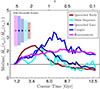 |
Fig. 10. Evolution of median relative accretion rates of each class across cosmic time. The underlying values were retrieved by calculating the ratio of accretion rates at 0.1 ⋅ Rvir and Rvir for each galaxy at each particle snapshot. Early-quenched galaxies exceed at accretion rates onto the center at high redshifts while abruptly decreasing after redshift z < 2. Main-sequence and late-quenched types have a similar evolution but with a clearly delayed peak. Rejuvenators do not peak but rather reach a plateau, while caught-types reach the same plateau after a strong delayed peak. |
Early-quenching galaxies exceed at funneling gas into the center in the early universe, while at later times not even all of inflowing gas onto the halo makes it into the galaxy. The high peak at early times (both in absolute flow rate, see Figure B.1, as well as significant mixing in the halo itself shown in Figure 10) may indicate a star burst at early times, which would both rapidly deplete as well as eject the gas, similar to what is shown by Kimmig et al. (2025).
With a delay the same behavior is displayed by late-quenching galaxies and even main-sequence-type galaxies. This means that all these galaxies to not predominantly cycle the same gas within their halos (where the ratio in Figure 10 would then be greater than 1), but instead approximately transport all or nearly all of the inflowing gas into the center, where it also remains. The difference is that for the quenched galaxies, this is practically no gas at all, while for the main sequence galaxies there is a significant amount, but the amount of transport from halo boundary to center is comparable among all three classes. Main-sequence-type galaxies thus do not cycle but simply accrete and retain, with long depletion times and little feedback to eject their gas again.
By contrast, caught- and rejuvenator-type galaxies set themselves apart from the other classes with median values higher by a factor of two toward z ≈ 0. This means that at all times they are cycling significant amounts of their gas within their own halo, potentially fueled by fountain processes that restore high accretion rates in the center while accretion at the halo outskirts declines. Cycling must on average then result in lower SFRs over the entirety of cosmic time, as the main-sequence-type galaxies are generally more massive than both the caught and rejuvenated galaxies.
In order to investigate how well the evolution of star formation rates is determined by gas accretion, we show in Figure 11 the agreement between the expected star formation obtained from the “bathtub” model using the measured gas accretion rates, and the real simulation output for the total galaxy sample across cosmic times. Note that we set the mass loading factor η to zero, as we directly measure the outflow rates, thus accounting for the contributions from AGN feedback and stellar feedback. The violins indicate the fractions of galaxies that have SFRs in agreement with expected values when using Equation (1). We find that the fraction of “bathtub”-like galaxies in the total galaxy sample (solid blue line) quickly rise and peak soon after z = 5. This means that at high redshifts, the assumed constant values for the return fraction R and depletion time tdepl of a dense GMC in a galaxy with a star formation efficiency of ϵff = 0.01 describe the transformation of accreted gas into stars well. Going toward lower redshift, then, the agreement drops. We note that there are more elaborate descriptions of the depletion timescale, such as a redshift-dependent description following the trend and offset to the SFMS ΔMS shown by Tacconi et al. (2020), yet it is noteworthy that our simple approach works well at high redshift.
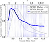 |
Fig. 11. Violin plot indicating the mean agreement of expectations from net accretion and the SFRs derived from Equation (1) with simulation output. An agreement is registered when both values deviate less than 0.5 dex from each other or for quenched galaxies, when simulation output and derived values return any SFR below 10−3 M⊙/yr. The vertical histograms (violins) count the agreement fraction of each galaxy within 500 Myr before and after each snapshot, combining three to four snapshot data points. This produces discretized fractions accumulating at 0.0, 0.25, 0.3, 0.5, 0.7, 0.75, and 1. The solid line follows the mean values within each bin. The blue dashed line shows the evolution of the SFR density of the galaxy sample normalized to the range of the figure. The black dashed line shows observational results for the evolution of the SFRD compiled by Madau & Dickinson (2014) and was normalized as well. |
The shape of this agreement is reminiscent of another well known relation. Thus, for comparison, we plot in arbitrary units (as we care about the shape and peak) the SFRD of the sample (dashed blue line), which peaks just before z = 2, in good agreement from the moment of SFRD peak according to observations (Madau & Dickinson 2014). We find a similar form, and slightly earlier peak, which may indicate that one of the reasons for the observed cosmic SFRD is the efficiency at which present gas can be converted into stars, with high-redshift galaxies following the “bathtub” model of direct conversion on short depletion times, while lower redshift galaxies grow increasingly inefficient. This is consistent with previous findings by Teklu et al. (2023) where the overall growth in size leads to lower SFRs with the same amount of cold gas available. In future work, we plan to more directly explore the link between the internal gas distribution of galaxies, a detailed characterization of their accretion flows (e.g., smoothness and angular momentum), and the resultant agreement with the “bathtub” model.
6. Environmental impact
It is well established that environment plays an important role for the star formation of satellites (Bahé et al. 2017; Lotz et al. 2019), but as we consider here only galaxies that remain as centrals until z ≈ 0 the picture is less clear. In this case, Remus & Kimmig (2025) and Kimmig et al. (2025) do find indications that the environment plays a crucial role both for quenching as well as for rejuvenation, at least at high redshifts. This can be understood as SFHs being dependent on both the availability of surrounding gas and the interaction with neighboring galaxies. A large number of lower-mass neighbors could fuel star formation through minor mergers, while higher-mass neighbors could steal away ejected or loosely bound gas and quench star formation in a similar fashion as for the Roche lobe of binary stars (e.g., Morris 1994).
Filaments have been proven as effective means to transport gas into the center while shielding against the quenching effect of a shock-heating hot halo (Dekel et al. 2009). While quenching can be induced by the intrinsic properties of a galaxy via hot halo and AGN, the frequent occurrence of rejuvenation processes suggests that the SFH is at least in part determined by the environment.
Seidel et al. (2025) have shown that the MAGNETICUM PATHFINDER simulations are well-suited to study gas flows between halos and their environments, finding agreement in the flow-rates across both box resolution and size. While the gas mass resolution here is not high enough to trace the evolution of individual molecular clouds, we well resolve the more massive gas flows that are needed to rejuvenate galaxies in the mass ranges considered in this work. We therefore searched for systematic differences between the environments of the classes with respect to the following two parameters:
-
The d5 parameter quantifies the density of the environment, defined as the minimum radius at which five neighboring galaxies, each with a total mass greater than 1011 M⊙, are found (Remus & Kimmig 2025).
-
The asphericity of gas infall at the virial radius. This parameter is derived by first performing a multipole expansion on the accretion rate distribution on a spherical shell and then calculating a ratio of the power of multipoles divided by the monopole power (Seidel et al., in prep.). Lower values (i.e., high monopole powers) correspond to isotropic accretion.
For the former, we find only mild differences, and as such refer the interested reader to Figure D.1 in the appendix for a further discussion. Here, we only briefly mention that caught galaxies tend toward slightly under-dense environments, while main-sequence-type show the opposite trend, with rejuvenated and quenched galaxies in the middle. However, these deviations are small, suggesting that our classes of galaxies are independent of the galaxy density of its environment.
Instead of this total density, it may be the geometry of the gas inflow. Indeed, we find a more pronounced difference between the classes when tracking how gas infall asphericities at their virial radii evolve. Figure 12 shows the evolution of median asphericities for each formation class as well as the underlying distributions as violins.
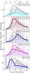 |
Fig. 12. Violin distributions of the evolution of asphericities for each class at each snapshot, with main sequence rejuvenators and quenched rejuvenators combined as “Rejuvenators”. The asphericity of gas infall is evaluated on the spherical surface of each virial radius. The solid lines follow the median of each snapshot. The dotted lines are the median distributions of the other classes for a direct comparison. The main-sequence types maintain lower values and therefore a predominantly spherical gas infall. The other classes display peaking distributions between redshifts 2 > z > 0.5. |
We find that galaxies that stay on the main sequence (cyan) also experience consistently isotropic infall throughout cosmic time, with only slightly higher asphericity between 2 > z > 0.5. The other classes undergo a pronounced peak of aspherical infall, each at a different redshift. Caught-type galaxies are the first class to peak in asphericity at z ≈ 2. Next are early-quenched galaxies that peak at z ≈ 1.2. Last to peak in asphericity as a group are the late-quenched galaxies at z ≈ 0.7. Rejuvenating galaxies peak at the same time as early-quenched galaxies, but with much lower total asphericity, indicating an infall history more similar to main-sequence-type galaxies.
This peaking distribution suggests a typical formation history of overall first isotropic infall, then a period of more filamentary accretion followed by a more isotropic flow that could reflect the buildup of halo fountains. Merger rates decline toward lower redshifts (O’Leary et al. 2021), such that increasing isotropy must be the result of smooth accretion. For the case of the main-sequence type galaxies, the rates are high enough (see Figure B.1) that this gas is likely the result of increasing amounts of ejected gas inflowing back from all directions. We will study this process of fountain build-up in more detail in a future study.
7. Summary and conclusions
We have traced the evolution of 1282 central galaxies in the highest-resolution box of the MAGNETICUM PATHFINDER cosmological hydrodynamical simulation suite through cosmic time while focusing on their gas inflow and star formation rates. By comparing their SFRs with respect to expectations from SFMS observations by Pearson et al. (2018), we identified moments of sustained quenching and rejuvenating and classified the formation histories accordingly.
We have found four characteristic formation pathways with respect to the SFR over cosmic time for central galaxies with M* > 1010 M⊙ at z ≈ 0:
-
Around 50% (646) of the galaxies quench soon after the peak of star formation at z ≈ 2, while 15% (187) quench later between 1 > z > 0.
-
Only 2% (22) evolve on the SFMS until z ≈ 0, where they make up 14% of the galaxies on the scaling relation. The other 86% has undergone quiescent periods.
-
Another 2% (20) of galaxies retain a lower but constant SFR and reappear on the main sequence when declining toward lower redshifts without need for rejuvenation.
-
A large fraction, 32% (407), of the galaxies undergo one or more cycles of rejuvenation on gigayear timescales, with 9% (117) of all galaxies returning onto the main sequence by z ≈ 0, while the other 23% (290) rejuvenate at some point but end up as quenched by z ≈ 0.
This means that the dominant fraction of galaxies (117 of 159) found on the SFMS at z ≈ 0 have undergone cycles of quenching and rejuvenation. These classes exist independent of which main sequence definition is used and for all main sequence definitions studied in this work (Speagle et al. 2014; Pearson et al. 2018; Leslie et al. 2020; Popesso et al. 2023), and only the relative frequencies per class change with definition.
These formation scenarios leave characteristic imprints on mean stellar ages and metallicities as well as the radial distribution of stellar ages. We find that rejuvenation generally takes place beyond the stellar half-mass radius. Galaxies that evolve along the main sequence consistently have the most efficient star formation in their very centers and the highest stellar metallicities. The final black hole masses at z ≈ 0 of main-sequence evolved galaxies and rejuvenating galaxies are distinctly lower than early-quenched galaxies at any given stellar mass, especially on the lower-mass end of the sample. Early formation conditions of efficient gas transport to the galaxies’ centers enhances not only star formation but also black hole growth, which in turn may impede rejuvenation or an evolution along the main sequence due to enhanced AGN feedback.
We also find that the scenarios emerge independent of the densities of galactic environments when looking at the d5 parameter, with no significant differences found between the formation classes across all redshifts. However, a clear distinction is possible when looking at the evolution of the asphericity of the infalling gas at the virial radii. Early and late quenching galaxies strongly peak in anisotropic accretion around the same time when their SFRs drop, which is in stark contrast to the absence of such an asphericity peak for main-sequence evolving galaxies. Explaining the physical reasons for this correlation is subject to future studies.
We compared the simulated star formation rates to predictions assuming mass conservation and a constant depletion time. The agreement between simulation results and expectations from gas flows evolves similar in shape and time to the evolution of the cosmic SFRD, with early redshifts showing the best agreement, which then declines toward lower redshifts. Consequently, at z > 2, the conditions of the Universe are described well by a simple description of star formation derived from gas flows and a depletion time of tdepl ≈ 0.5 Gyr. After that time, the conditions change, as only about 40% of the SFRs of galaxies are consistent with expectations from the “bathtub” model equation, which may be due to a more complex phase where star formation is less dependent on the net gas accretion and additional physical processes (heating, turbulence, dry mergers) become more dominant in regulating star formation.
We conclude that galaxies evolving consistently along the main sequence are relatively rare. Most current day main sequence galaxies have undergone one or multiple cycles of quiescence and rejuvenation.
Acknowledgments
We thank the referee for their valuable feedback which helped with clarification and context of the results. This work was performed at the LMU Munich with the support by the Excellence Cluster ORIGINS. The MAGNETICUM simulations were performed at the Leibniz-Rechenzentrum with CPU time assigned to the Project pr83li. This work was supported by the Deutsche Forschungsgemeinschaft (DFG, German Research Foundation) under Germany’s Excellence Strategy – EXC 2094 – 390783311. We are especially grateful for the support by M. Petkova through the Computational Center for Particle and Astrophysics (C2PAP). LCK acknowledges support by the DFG project nr. 516355818. KD acknowledges support by the COMPLEX project from the European Research Council (ERC) under the European Union’s Horizon 2020 research and innovation program grant agreement ERC-2019-AdG 882679.
References
- Arth, A., Dolag, K., Beck, A. M., Petkova, M., & Lesch, H. 2014, ArXiv e-prints [arXiv:1412.6533] [Google Scholar]
- Bahé, Y. M., Barnes, D. J., Dalla Vecchia, C., et al. 2017, MNRAS, 470, 4186 [Google Scholar]
- Balogh, M. L., Baldry, I. K., Nichol, R., et al. 2004, ApJ, 615, L101 [Google Scholar]
- Beck, A. M., Murante, G., Arth, A., et al. 2016, MNRAS, 455, 2110 [Google Scholar]
- Behroozi, P. S., Wechsler, R. H., & Conroy, C. 2013, ApJ, 770, 57 [NASA ADS] [CrossRef] [Google Scholar]
- Birnboim, Y., & Dekel, A. 2003, MNRAS, 345, 349 [Google Scholar]
- Bouché, N., Dekel, A., Genzel, R., et al. 2010, ApJ, 718, 1001 [Google Scholar]
- Brinchmann, J., Charlot, S., White, S. D. M., et al. 2004, MNRAS, 351, 1151 [Google Scholar]
- Bruzual, G., & Charlot, S. 2003, MNRAS, 344, 1000 [NASA ADS] [CrossRef] [Google Scholar]
- Bullock, J. S., & Boylan-Kolchin, M. 2017, ARA&A, 55, 343 [Google Scholar]
- Burkert, A. 2017, Mem. Soc. Astron. Ital., 88, 533 [Google Scholar]
- Carnall, A. C., Walker, S., McLure, R. J., et al. 2020, MNRAS, 496, 695 [Google Scholar]
- Chabrier, G. 2003, PASP, 115, 763 [Google Scholar]
- Chauke, P., van der Wel, A., Pacifici, C., et al. 2019, ApJ, 877, 48 [NASA ADS] [CrossRef] [Google Scholar]
- Chevance, M., Krumholz, M. R., McLeod, A. F., et al. 2023, ASP Conf. Ser., 534, 1 [NASA ADS] [Google Scholar]
- Dekel, A., & Birnboim, Y. 2006, MNRAS, 368, 2 [NASA ADS] [CrossRef] [Google Scholar]
- Dekel, A., & Birnboim, Y. 2008, MNRAS, 383, 119 [Google Scholar]
- Dekel, A., & Silk, J. 1986, ApJ, 303, 39 [Google Scholar]
- Dekel, A., Birnboim, Y., Engel, G., et al. 2009, Nature, 457, 451 [Google Scholar]
- Di Matteo, T., Springel, V., & Hernquist, L. 2005, Nature, 433, 604 [NASA ADS] [CrossRef] [Google Scholar]
- Dolag, K., Jubelgas, M., Springel, V., Borgani, S., & Rasia, E. 2004, ApJ, 606, L97 [NASA ADS] [CrossRef] [Google Scholar]
- Dolag, K., Vazza, F., Brunetti, G., & Tormen, G. 2005, MNRAS, 364, 753 [NASA ADS] [CrossRef] [Google Scholar]
- Dolag, K., Borgani, S., Murante, G., & Springel, V. 2009, MNRAS, 399, 497 [Google Scholar]
- Dolag, K., Mevius, E., & Remus, R.-S. 2017, Galaxies, 5, 35 [NASA ADS] [CrossRef] [Google Scholar]
- Dolag, K., Remus, R. S., Valenzuela, L. M., et al. 2025, ArXiv e-prints [arXiv:2504.01061] [Google Scholar]
- Donnari, M., Pillepich, A., Nelson, D., et al. 2019a, MNRAS, 489, 3036 [NASA ADS] [CrossRef] [Google Scholar]
- Donnari, M., Pillepich, A., Nelson, D., et al. 2019b, MNRAS, 485, 4817 [Google Scholar]
- Donnert, J., Dolag, K., Brunetti, G., & Cassano, R. 2013, MNRAS, 429, 3564 [Google Scholar]
- Efstathiou, G. 2000, MNRAS, 317, 697 [NASA ADS] [CrossRef] [Google Scholar]
- Ellison, S. L., Wilkinson, S., Woo, J., et al. 2022, MNRAS, 517, L92 [NASA ADS] [CrossRef] [Google Scholar]
- Fabian, A. C., & Nulsen, P. E. J. 1977, MNRAS, 180, 479 [NASA ADS] [CrossRef] [Google Scholar]
- Fabjan, D., Borgani, S., Tornatore, L., et al. 2010, MNRAS, 401, 1670 [Google Scholar]
- Ferland, G. J., Korista, K. T., Verner, D. A., et al. 1998, PASP, 110, 761 [Google Scholar]
- Franx, M., van Dokkum, P. G., Förster Schreiber, N. M., et al. 2008, ApJ, 688, 770 [NASA ADS] [CrossRef] [Google Scholar]
- Gómez-Guijarro, C., Elbaz, D., Xiao, M., et al. 2022, A&A, 659, A196 [NASA ADS] [CrossRef] [EDP Sciences] [Google Scholar]
- González Villalba, J. A., Dolag, K., & Biffi, V. 2025, A&A, 694, A232 [NASA ADS] [CrossRef] [EDP Sciences] [Google Scholar]
- Haardt, F., & Madau, P. 2001, in Clusters of Galaxies and the High Redshift Universe Observed in X-rays, eds. D. M. Neumann, & J. T. V. Tran, 64 [Google Scholar]
- Hao, C.-N., Xia, X., Shi, Y., et al. 2024, ApJ, 968, 3 [NASA ADS] [CrossRef] [Google Scholar]
- Heiderman, A., Evans, N. J., II, Allen, L. E., Huard, T., & Heyer, M. 2010, ApJ, 723, 1019 [Google Scholar]
- Hirschmann, M., Dolag, K., Saro, A., et al. 2014, MNRAS, 442, 2304 [Google Scholar]
- Jeans, J. H. 1902, Phil. Trans. Roy. Soc. London Ser. A, 199, 1 [CrossRef] [Google Scholar]
- Kimmig, L. C., Remus, R.-S., Seidel, B., et al. 2025, ApJ, 979, 15 [Google Scholar]
- Komatsu, E., Smith, K. M., Dunkley, J., et al. 2011, ApJS, 192, 18 [Google Scholar]
- Kormendy, J., & Ho, L. C. 2013, ARA&A, 51, 511 [Google Scholar]
- Kroupa, P. 2001, MNRAS, 322, 231 [NASA ADS] [CrossRef] [Google Scholar]
- Krumholz, M. R., & McKee, C. F. 2005, ApJ, 630, 250 [Google Scholar]
- Krumholz, M. R., & Tan, J. C. 2007, ApJ, 654, 304 [NASA ADS] [CrossRef] [Google Scholar]
- Krumholz, M. R., Dekel, A., & McKee, C. F. 2012, ApJ, 745, 69 [Google Scholar]
- Kudritzki, R.-P., Teklu, A. F., Schulze, F., et al. 2021, ApJ, 910, 87 [NASA ADS] [CrossRef] [Google Scholar]
- Lada, C. J., Lombardi, M., & Alves, J. F. 2010, ApJ, 724, 687 [Google Scholar]
- Leitner, S. N., & Kravtsov, A. V. 2011, ApJ, 734, 48 [NASA ADS] [CrossRef] [Google Scholar]
- Leslie, S. K., Schinnerer, E., Liu, D., et al. 2020, ApJ, 899, 58 [Google Scholar]
- Lilly, S. J., Carollo, C. M., Pipino, A., Renzini, A., & Peng, Y. 2013, ApJ, 772, 119 [NASA ADS] [CrossRef] [Google Scholar]
- Lin, L., Pan, H.-A., Ellison, S. L., et al. 2024, ApJ, 963, 115 [NASA ADS] [CrossRef] [Google Scholar]
- Lotz, M., Remus, R.-S., Dolag, K., Biviano, A., & Burkert, A. 2019, MNRAS, 488, 5370 [NASA ADS] [CrossRef] [Google Scholar]
- Lustig, P., Strazzullo, V., Remus, R.-S., et al. 2023, MNRAS, 518, 5953 [Google Scholar]
- Madau, P., & Dickinson, M. 2014, ARA&A, 52, 415 [Google Scholar]
- Masters, K. L., Mosleh, M., Romer, A. K., et al. 2010, MNRAS, 405, 783 [NASA ADS] [Google Scholar]
- McKee, C. F., & Ostriker, E. C. 2007, ARA&A, 45, 565 [Google Scholar]
- Mitchell, P. D., Schaye, J., Bower, R. G., & Crain, R. A. 2020, MNRAS, 494, 3971 [Google Scholar]
- Morris, S. L. 1994, PASP, 106, 154 [Google Scholar]
- Noeske, K. G., Weiner, B. J., Faber, S. M., et al. 2007, ApJ, 660, L43 [CrossRef] [Google Scholar]
- O’Leary, J. A., Moster, B. P., Naab, T., & Somerville, R. S. 2021, MNRAS, 501, 3215 [Google Scholar]
- Oppenheimer, B. D., & Davé, R. 2008, MNRAS, 387, 577 [NASA ADS] [CrossRef] [Google Scholar]
- Pearson, W. J., Wang, L., Hurley, P. D., et al. 2018, A&A, 615, A146 [NASA ADS] [CrossRef] [EDP Sciences] [Google Scholar]
- Piotrowska, J. M., Bluck, A. F. L., Maiolino, R., & Peng, Y. 2022, MNRAS, 512, 1052 [NASA ADS] [CrossRef] [Google Scholar]
- Popesso, P., Concas, A., Cresci, G., et al. 2023, MNRAS, 519, 1526 [Google Scholar]
- Rees, M. J., & Ostriker, J. P. 1977, MNRAS, 179, 541 [NASA ADS] [CrossRef] [Google Scholar]
- Remus, R.-S., & Forbes, D. A. 2022, ApJ, 935, 37 [NASA ADS] [CrossRef] [Google Scholar]
- Remus, R.-S., & Kimmig, L. C. 2025, ApJ, 982, 30 [Google Scholar]
- Santini, P., Fontana, A., Castellano, M., et al. 2017, ApJ, 847, 76 [NASA ADS] [CrossRef] [Google Scholar]
- Sarazin, C. L. 1986, Rev. Mod. Phys., 58, 1 [Google Scholar]
- Schechter, P. 1976, ApJ, 203, 297 [Google Scholar]
- Schulze, F., Remus, R.-S., Dolag, K., et al. 2018, MNRAS, 480, 4636 [Google Scholar]
- Seidel, B. A., Remus, R.-S., Valenzuela, L. M., Kimmig, L. C., & Dolag, K. 2025, A&A, 701, A192 [NASA ADS] [CrossRef] [EDP Sciences] [Google Scholar]
- Shakura, N. I., & Sunyaev, R. A. 1973, A&A, 24, 337 [NASA ADS] [Google Scholar]
- Speagle, J. S., Steinhardt, C. L., Capak, P. L., & Silverman, J. D. 2014, ApJS, 214, 15 [Google Scholar]
- Spitzer, L. 1962, Physics of Fully Ionized Gases (New York: Interscience) [Google Scholar]
- Springel, V. 2005, MNRAS, 364, 1105 [Google Scholar]
- Springel, V., & Hernquist, L. 2003, MNRAS, 339, 289 [Google Scholar]
- Springel, V., Yoshida, N., & White, S. D. M. 2001a, New Astron., 6, 79 [Google Scholar]
- Springel, V., White, S. D. M., Tormen, G., & Kauffmann, G. 2001b, MNRAS, 328, 726 [Google Scholar]
- Springel, V., Di Matteo, T., & Hernquist, L. 2005, MNRAS, 361, 776 [Google Scholar]
- Strateva, I., Ivezić, Ž., Knapp, G. R., et al. 2001, AJ, 122, 1861 [CrossRef] [Google Scholar]
- Tacchella, S., Dekel, A., Carollo, C. M., et al. 2016, MNRAS, 457, 2790 [Google Scholar]
- Tacconi, L. J., Genzel, R., & Sternberg, A. 2020, ARA&A, 58, 157 [NASA ADS] [CrossRef] [Google Scholar]
- Tanaka, T. S., Shimasaku, K., Tacchella, S., et al. 2024, PASJ, 76, 1 [Google Scholar]
- Teklu, A. F., Remus, R.-S., Dolag, K., et al. 2015, ApJ, 812, 29 [Google Scholar]
- Teklu, A. F., Remus, R.-S., Dolag, K., & Burkert, A. 2017, MNRAS, 472, 4769 [NASA ADS] [CrossRef] [Google Scholar]
- Teklu, A., Kudritzki, R.-P., Dolag, K., Remus, R.-S., & Kimmig, L. 2023, ApJ, 954, 182 [NASA ADS] [CrossRef] [Google Scholar]
- Tornatore, L., Borgani, S., Springel, V., et al. 2003, MNRAS, 342, 1025 [NASA ADS] [CrossRef] [Google Scholar]
- Tornatore, L., Borgani, S., Dolag, K., & Matteucci, F. 2007, MNRAS, 382, 1050 [Google Scholar]
- Trussler, J. A. A., Conselice, C. J., Adams, N., et al. 2025, MNRAS, 537, 3662 [Google Scholar]
- Tumlinson, J., Peeples, M. S., & Werk, J. K. 2017, ARA&A, 55, 389 [Google Scholar]
- Utomo, D., Sun, J., Leroy, A. K., et al. 2018, ApJ, 861, L18 [NASA ADS] [CrossRef] [Google Scholar]
- Valenzuela, L. M., Remus, R.-S., Dolag, K., & Seidel, B. A. 2024, A&A, 690, A206 [NASA ADS] [CrossRef] [EDP Sciences] [Google Scholar]
- van de Sande, J., Lagos, C. D. P., Welker, C., et al. 2019, MNRAS, 484, 869 [NASA ADS] [CrossRef] [Google Scholar]
- van de Weygaert, R., & Bond, J. R. 2008, in A Pan-Chromatic View of Clusters of Galaxies and the Large-Scale Structure, eds. M. Plionis, O. López-Cruz, & D. Hughes, 740, 335 [NASA ADS] [CrossRef] [Google Scholar]
- Whitaker, K. E., van Dokkum, P. G., Brammer, G., & Franx, M. 2012, ApJ, 754, L29 [Google Scholar]
- Wiersma, R. P. C., Schaye, J., Theuns, T., Dalla Vecchia, C., & Tornatore, L. 2009, MNRAS, 399, 574 [NASA ADS] [CrossRef] [Google Scholar]
- Wyder, T. K., Martin, D. C., Schiminovich, D., et al. 2007, ApJS, 173, 293 [Google Scholar]
- Yi, S. K., Yoon, S. J., Kaviraj, S., et al. 2005, ApJ, 619, L111 [NASA ADS] [CrossRef] [Google Scholar]
- Zhang, J., Li, Y., Leja, J., et al. 2023, ApJ, 952, 6 [NASA ADS] [CrossRef] [Google Scholar]
Appendix A: Varying the smoothing window
Numbers of galaxies within each formation class with respect to expectations according to the SFMS as found by Pearson et al. (2018).
We classify evolution scenarios as shown by representative examples in Figure 2 algorithmically. In order to tie the SFRs to gas flows we applied a smoothing window of one gigayear to the simulation output representing the depletion timescale. The depletion timescale roughly determines how fast a galaxy globally reacts to change in gas flows according to the “bathtub” model (Equation 1).
In order to check for robustness, we applied the algorithm using also a 0.5 and a 1.5 Gyr time window. The effect on sample sizes is shown in Table A.1. Larger smoothing windows disregard short-term fluctuations of SFRs. As a consequence, more galaxies are considered main-sequence or quenched. Those would otherwise have been attributed to the group of rejuvenating galaxies, as short-term fluctuations would have been considered quenching and rejuvenating processes. The number of caught-type galaxies remains stable, as they have been classified manually. However, despite the varying class member numbers, each class roughly maintains its size, showing these characteristic evolution pathways emerge for a range of smoothing window size choices.
Appendix B: Gas flows
We tested the link between gas flows and star formation by deriving the latter from flow rates and simplifying assumptions. The median net accretion rate evolution used for the derivation is shown in Figure B.1. Specifically, we normalize each galaxy’s net accretion rate by respective expected accretion rate (Dekel et al. 2009) and then calculate class median values at each snapshot across cosmic time. When comparing the median net accretion rates onto the galaxies at 0.1 Rvir (solid lines) for to the values at the virial radii (dashed lines) for each class, the figure shows that net gas accretion evolves similar at both radii. While main-sequence (cyan), caught (blue) and rejuvenator (magenta) type galaxies sustain positive net accretion rates roughly on the order of expectations from dark matter assembly (Dekel et al. 2009, dashed vertical line), quenching galaxies (dark red and dark blue) transition to even slightly negative values. Notably, the main-sequence type galaxies (cyan) have consistently higher values at the virial radii than at the galaxy borders.
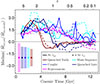 |
Fig. B.1. Median net gas accretion history evolution of each formation class across cosmic time. We show the net accretion rates at the virial radii as dashed lines and as solid lines accretion rates onto the center of the halos at ten percent virial radius. Prior to combining the data, we normalized each accretion rate value by halo mass and redshift according to expectations from dark-matter assembly (Dekel et al. 2009). The horizontal dashed black line at a value of one highlights this expectation by definition. The median of main-sequence galaxies are in cyan, quenched in dark red, rejuvenating galaxies in magenta and caught galaxies in blue colors. The vertical bars outline a representative 50th percentile scatter. On average, accretion rates generally do not differ too much from the expectations. Quenching galaxies collectively assume negative values correlating with the time of quenching of their star formation. This correlation becomes evident from comparing the early- and late-quenching galaxy populations. |
All galaxies tend to decline in net accretion toward lower redshifts. Quenched-type galaxies show the largest offset by having a clear peak at high redshifts and then dropping even below zero at lower redshifts. Main-sequence types also peak early but never drop as much, and always stay among the highest accretion rates. Rejuvenators peak later and less high. Caught-type galaxies maintain very high net accretion rates for a longer time compared to expectations from their halo masses.
Due to higher overall densities and velocities, the infall rates are higher in the centers of halos while all classes achieve lower and similar values at their virial radii. The central inflow rates at ten percent of each virial radius of quenched-type galaxies drops severely off the total sample toward lower redshifts, which is consistent with their net accretion.
Appendix C: Influence of AGN feedback
Piotrowska et al. (2022) have shown that AGN feedback quenching is strongly related to the mass of supermassive black holes in the centers of galaxies. We therefore show in Figure C.1 the black hole masses and stellar masses of each galaxy at z ≈ 0 colored according to its star formation evolution class to estimate the influence of AGN feedback on the evolution scenarios. At any given stellar mass, quenched galaxies (dark red and dark blue circles) occupy the highest black hole masses. This is likely due to how gas flows onto the central black hole, with high-z environments creating more isotropic flows (Kimmig et al. 2025, Seidel et al. in prep), while galaxies that make a majority of their stars at later times or in on-off cycles do not as efficiently funnel the gas toward the center. This leads to lower black hole masses, with the most extreme case found for those evolving along the main sequence. We posit that galaxies that solely grew along the main sequence are the result of higher angular momentum gas that forms its stars in a disk without strongly feeding the central supermassive black hole.
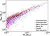 |
Fig. C.1. MBH-M* relation of the galaxy sample at z ≈ 0. Especially for the mass range of 1010M⊙ ≤ M⊙ ≤ 1011M⊙, a clear transition order from quenched galaxies along the Magorrian relation to lower black hole masses for star-forming galaxies. Specifically, early-quenched galaxies (dark red) have the highest values, followed by late-quenched (dark blue), rejuvenated quenched (lilac), MS-evolved (cyan), and finally rejuvenated main-sequence (pink) galaxies as well as caught-type galaxies (blue) at the lower black hole mass end. |
Appendix D: Environment with the d5 parameter
In section 6, we have discussed a clear correlation between gas inflow geometry at the halo outskirts and star formation rate evolution. While this shows that the environment plays an important role in the star formation evolution of a galaxy, the d5 parameter is an unsuitable tracer of environment. We show in Figure D.1 the evolution of median d5 parameters for each class across cosmic time and find that, independent of redshift, the d5 parameter barely varies between the classes. Only the smallest classes of main-sequence- and caught-type galaxies appear to reside in differently populated environments. Main-sequence galaxies tend to higher densities and caught-type galaxies to lower. This suggests that a denser environment neighboring galaxies only impacts the median sSFR but not quenching or rejuvenation. However, the differences are overall minuscule compared to the dominating overlap of violins.
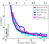 |
Fig. D.1. Evolution of the class median d5 parameter values (Remus & Kimmig 2025) across cosmic time. Lower values indicate a denser environment of a galaxy. We chose comoving coordinates for a better comparison between across cosmic time. The 50th percentile scatter range shown in gray in the bottom left corner is similar for all classes and cosmic cosmic time. All classes show a very similar evolution with only faint differences with main-sequence types residing in denser environments consistently and caught-types found in less dense environments. |
All Tables
Number of galaxies within each formation class with respect to expectations according to a list of results for the SFMS.
Numbers of galaxies within each formation class with respect to expectations according to the SFMS as found by Pearson et al. (2018).
All Figures
|
Fig. 1. Star formation main sequence at z ≈ 0. The left- and right-hand panels show the results with respect to two selection criteria for MAGNETICUM galaxies. By imposing a threshold of sSFR > 0.2/tHub (left), as used by Carnall et al. (2020) (dashed black line), we find a slightly higher linear fit to the logarithmic values (dashed blue line) compared to selecting for all kinematic disks with SFR > 0 M⊙/yr (right). Results from observations are displayed in magenta, simulations are shown in blue colors. The solid blue line and shaded region show the running median and 50th percentile region. The circles represent the galaxies from the MAGNETICUM PATHFINDER simulations colored according to their morphology as defined by the b-value (Teklu et al. 2015). Gray circles are ignored for the running median lines on each panel. The SFR values below the range of the figure are fixed to the bottom to represent the full sample in this work. The magenta solid line and shaded region highlights a range of ±0.5 dex around the main sequence fit by Pearson et al. (2018), which we used in this work to distinguish between being on and off the main sequence. The other magenta lines are additional observational results: dashed line (Speagle et al. 2014), dash-dotted line (Leslie et al. 2020), and dotted line (Popesso et al. 2023). The dashed cyan line marks the results from ILLUSTRISTNG by Donnari et al. (2019a). |
| In the text | |
|
Fig. 2. Examples of the four formation scenarios for galaxies with respect to sSFR changes over time. The black lines and shades indicate the main sequence values depending on the redshift and stellar mass of a galaxy according to results by Pearson et al. (2018) with a scatter of ±0.5 dex applied to differentiate between on or off the main sequence. From top to bottom, the panels show a main-sequence-type galaxy (cyan), an early-quenched galaxy (dark red), a rejuvenating galaxy (magenta), and a caught galaxy (blue). Two classes are not explicitly represented here. First, the “late-quenched” types only differ from the “early-quenched” by dropping off the main sequence after redshift z = 1. Second, rejuvenator-main-sequence-type galaxies recover a stable position on the main sequence at redshift z = 0, unlike rejuvenator-quenched-type galaxies, which also go through rejuvenation cycles but do not end up on the main sequence. The vertical lines highlight the snapshots corresponding to each row in Figure 3. |
| In the text | |
|
Fig. 3. Star formation main sequence evolution of the MAGNETICUM galaxies traced back from the selection made at z = 0 (bottom-row panels). The rows contain snapshots with decreasing redshift from top to bottom between 6 < z < 0. From left to right, the different sub-samples “Main Sequence”, “Quenched”, “Rejuvenator”, and “Caught” are highlighted by colors in front of the total sample in gray in the background. Light blue data points represent galaxies that have not yet dropped below the main sequence; each quenching event is counted and encoded in the changing color of the data points as red (once), orange (twice), and yellow (three times). The large points are the cherry-picked representative galaxies from Figure 2. Quenched representative galaxies are set as half-circles to the bottom of the panels for visibility. The black line and gray shades correspond to the main-sequence found by Pearson et al. (2018). Gray contours outline the distribution of the full galaxy sample for comparison in each panel. |
| In the text | |
|
Fig. 4. Similar to Figure 2 but focused on the difference between the subclass pairs of early- and late-quenched galaxies as well as quenched and main-sequence rejuvenators. The colored dashed lines represent the cases also shown in Figure 2, while the colored solid lines are the subtypes to differentiate. The gray dashed quiescence criteria (Carnall et al. 2020) and black-shaded SFMS expectations (Pearson et al. 2018) are derived from the stellar masses of the latter. This causes the pink dashed main-sequence-rejuvenator to not lie on the SFMS at z ≈ 0 due to the larger stellar mass (see Figure 5) and therefore lower sSFR. The early-quenched galaxy does recover star formation after quenching but never consistently makes it back onto the main sequence. The late-quenched galaxy also almost makes a passive rejuvenation akin to caught-type galaxies, since the main sequence drops at z < 0.5. However, it is still mostly more than 0.5 dex below the main sequence averaged over a smoothing window of one gigayear, ruling out a rejuvenation scenario. The main-sequence rejuvenator undergoes a more pronounced quenched phase than the quenched rejuvenator. |
| In the text | |
|
Fig. 5. Similar to Figure 3 but focused on the difference between the subclass pairs of early- and late-quenched galaxies as well as quenched and main-sequence rejuvenators. Here, the colors refer to the subclass types instead of quenching incidents. The large points show the cherry-picked representative galaxies from Figure 4, again set to the bottom of the panels as half-circles for visibility in case of low SFR values. By construction, the difference between early- and late-quenched is most pronounced at z = 1. At z ≈ 0, the non-zero distributions are barely noticeable. Analogously, the difference between the two rejuvenator subclasses is the sharpest at z ≈ 0. Both subclasses undergo rejuvenation cycles at different times, but the relation to the SFMS determines the classification. |
| In the text | |
|
Fig. 6. Median radial profiles and 68th percentile spread of stellar ages at z = 0. Before extracting the running median and scatter, we calculated the mean stellar ages for each galaxy in nine equal-width radial bins between 0 and 5 R1/2. The solid lines and shaded regions correspond to the statistics of the class indicated at the top of each panel. The dashed lines are the running medians from the panels to the left of each panel for a direct comparison. Higher values correspond to an older population, which is fairly constant at around ten gigayears for early-quenched galaxies. Main-sequence-type galaxies show increasingly young populations toward the center, while the three types of rejuvenating classes are the youngest at roughly one half-mass radius and increase in age again toward the very center as well as the outskirts. |
| In the text | |
|
Fig. 7. Mean metallicities and ages of the full galaxy sample at z = 0. Less populated classes are in front of larger ones for visibility while slightly decreasing the perceived scatter of the larger classes, such as the early-quenched galaxy class. This class concentrates at high ages and lower metallicities opposing main-sequence types. The intermediate classes of late-quenchers and rejuvenating galaxies bridge the gap in a dichotomous way of age and metallicity combination. |
| In the text | |
|
Fig. 8. Mean stellar abundance ratios of the galaxy sample at z ≈ 0. Oxygen was chosen to represent α enrichment. Akin to Figure 7, different regions of the diagram are predominantly occupied by specific classes. A clear gradient emerges from the top left to the bottom right of the distribution as QE-QL-RQ-Ct-RM-MS. Main-sequence-type galaxies tend to the right-most corner of the distribution. |
| In the text | |
|
Fig. 9. Fractions of formation class members in stellar mass bins at z ≈ 0. Slight shifts of data points originate from taking the median stellar masses instead of bin centers. Early-quenched galaxies (dark red) peak at around M* = 1011, while late-quenched ones (dark blue) peak at slightly higher masses. Galaxies with rejuvenation cycles (dashed magenta line) in their formation histories are more prevalent on the lower- and higher-mass ends of the range between 1010 M⊙ ≤ M* ≤ 1012 M⊙. Quenched rejuvenators (lilac) tend more toward lower masses, while a rejuvenation sustained until z ≈ 0 (pink) is more often found at higher masses. Main-sequence (cyan) and caught types (blue) are generally rare with a faint preference for the high-mass end. Both subtypes are more prevalent on the lower- and higher- mass ends of the range between 1010 M⊙ ≤ M* ≤ 1012 M⊙. |
| In the text | |
|
Fig. 10. Evolution of median relative accretion rates of each class across cosmic time. The underlying values were retrieved by calculating the ratio of accretion rates at 0.1 ⋅ Rvir and Rvir for each galaxy at each particle snapshot. Early-quenched galaxies exceed at accretion rates onto the center at high redshifts while abruptly decreasing after redshift z < 2. Main-sequence and late-quenched types have a similar evolution but with a clearly delayed peak. Rejuvenators do not peak but rather reach a plateau, while caught-types reach the same plateau after a strong delayed peak. |
| In the text | |
|
Fig. 11. Violin plot indicating the mean agreement of expectations from net accretion and the SFRs derived from Equation (1) with simulation output. An agreement is registered when both values deviate less than 0.5 dex from each other or for quenched galaxies, when simulation output and derived values return any SFR below 10−3 M⊙/yr. The vertical histograms (violins) count the agreement fraction of each galaxy within 500 Myr before and after each snapshot, combining three to four snapshot data points. This produces discretized fractions accumulating at 0.0, 0.25, 0.3, 0.5, 0.7, 0.75, and 1. The solid line follows the mean values within each bin. The blue dashed line shows the evolution of the SFR density of the galaxy sample normalized to the range of the figure. The black dashed line shows observational results for the evolution of the SFRD compiled by Madau & Dickinson (2014) and was normalized as well. |
| In the text | |
|
Fig. 12. Violin distributions of the evolution of asphericities for each class at each snapshot, with main sequence rejuvenators and quenched rejuvenators combined as “Rejuvenators”. The asphericity of gas infall is evaluated on the spherical surface of each virial radius. The solid lines follow the median of each snapshot. The dotted lines are the median distributions of the other classes for a direct comparison. The main-sequence types maintain lower values and therefore a predominantly spherical gas infall. The other classes display peaking distributions between redshifts 2 > z > 0.5. |
| In the text | |
|
Fig. B.1. Median net gas accretion history evolution of each formation class across cosmic time. We show the net accretion rates at the virial radii as dashed lines and as solid lines accretion rates onto the center of the halos at ten percent virial radius. Prior to combining the data, we normalized each accretion rate value by halo mass and redshift according to expectations from dark-matter assembly (Dekel et al. 2009). The horizontal dashed black line at a value of one highlights this expectation by definition. The median of main-sequence galaxies are in cyan, quenched in dark red, rejuvenating galaxies in magenta and caught galaxies in blue colors. The vertical bars outline a representative 50th percentile scatter. On average, accretion rates generally do not differ too much from the expectations. Quenching galaxies collectively assume negative values correlating with the time of quenching of their star formation. This correlation becomes evident from comparing the early- and late-quenching galaxy populations. |
| In the text | |
|
Fig. C.1. MBH-M* relation of the galaxy sample at z ≈ 0. Especially for the mass range of 1010M⊙ ≤ M⊙ ≤ 1011M⊙, a clear transition order from quenched galaxies along the Magorrian relation to lower black hole masses for star-forming galaxies. Specifically, early-quenched galaxies (dark red) have the highest values, followed by late-quenched (dark blue), rejuvenated quenched (lilac), MS-evolved (cyan), and finally rejuvenated main-sequence (pink) galaxies as well as caught-type galaxies (blue) at the lower black hole mass end. |
| In the text | |
|
Fig. D.1. Evolution of the class median d5 parameter values (Remus & Kimmig 2025) across cosmic time. Lower values indicate a denser environment of a galaxy. We chose comoving coordinates for a better comparison between across cosmic time. The 50th percentile scatter range shown in gray in the bottom left corner is similar for all classes and cosmic cosmic time. All classes show a very similar evolution with only faint differences with main-sequence types residing in denser environments consistently and caught-types found in less dense environments. |
| In the text | |
Current usage metrics show cumulative count of Article Views (full-text article views including HTML views, PDF and ePub downloads, according to the available data) and Abstracts Views on Vision4Press platform.
Data correspond to usage on the plateform after 2015. The current usage metrics is available 48-96 hours after online publication and is updated daily on week days.
Initial download of the metrics may take a while.