| Issue |
A&A
Volume 704, December 2025
|
|
|---|---|---|
| Article Number | A274 | |
| Number of page(s) | 19 | |
| Section | Catalogs and data | |
| DOI | https://doi.org/10.1051/0004-6361/202555251 | |
| Published online | 19 December 2025 | |
Magnetic activity of M dwarf stars from the LAMOST DR10 medium-resolution survey
1
College of Physics, Guizhou University,
550025
Guiyang,
PR China
2
Dept. of Physics and Astronomy and SARA, Butler University,
Indianapolis,
IN
46208,
USA
3
Department of Physics & Astronomy Howard University,
Washington,
DC
20059,
USA
★ Corresponding author: This email address is being protected from spambots. You need JavaScript enabled to view it.
Received:
22
April
2025
Accepted:
28
September
2025
Abstract
Aims. M dwarf stars (red dwarfs) are the most common stars in the Milky Way (70% of all stars). Their temperatures and masses are low, but their magnetic activity is strong and includes flares, starspots, and coronal mass ejections. The internal structure and evolutionary processes of stars can be understood by studying their magnetic activity, as can their effect on the environments of surrounding planets. We used medium-resolution spectrum data of M dwarf stars from Data Release 10 (DR10) of the Large Sky Area Multi-Object Fiber Spectroscopic Telescope (LAMOST) to conduct a comprehensive and in-depth investigation of the stellar magnetic activity, flare, and starspot variations.
Methods. By cross-matching the low-resolution spectrum M dwarf star catalog from LAMOST DR10 medium-resolution spectrum data, we successfully identified 20 279 M dwarfs and obtained a total of 708 969 datasets of medium-resolution spectrum. These data provide a rich foundation for studying stellar magnetic fields and activity characteristics. Additionally, we cross-matched the data with light curves from the Transiting Exoplanet Survey Satellite (TESS), from which we acquired light-curve data for 2868 stars. We identified 891 flare stars in this sample, which provide an important sample for the statistical characteristics and physical mechanisms of flare events. By combining them with Gaia data, we clarified the characterisspatial distribution characteristics of M dwarfs in the Milky Way.
Results. Statistical studies of the magnetic activity of M dwarf stars based on LAMOST medium-resolution spectrum, showed that as the effective temperature of M dwarf stars increases, their stellar activity diminishes, although this trend becomes less evident for Teff > 3600 K, and the amplitude of Hα line variations increases strongly for later spectral types. In a sample of 11 868 M dwarfs with a signal-to-noise ratio higher than 10, we found that 1676 of the stars exhibited Hα emission features, that is, were active stars. In the 891 flare stars identified from TESS light-curve data, we also detected 7496 flare events. Twenty-five of the 119 stars had EWHα flare-like variations in TESS light-curve data. Research also clarified that the activity of M dwarf stars in the Milky Way decreases with increasing vertical distance from the Galactic disk. Furthermore, by combining LAMOST spectrum surveys with TESS light-curve data, a positive correlation between chromospheric activity as indicated by Hα lines and the starspot area was established. Additionally, studies showed a positive correlation between the flare energy and their duration in M dwarf stars, and the slope of this correlation decreases for later spectral types. Finally, through analyzing the asymmetry of Hα lines, two candidate coronal mass ejections were identified.
Key words: catalogs / surveys / stars: activity / stars: chromospheres
© The Authors 2025
 Open Access article, published by EDP Sciences, under the terms of the Creative Commons Attribution License (https://creativecommons.org/licenses/by/4.0), which permits unrestricted use, distribution, and reproduction in any medium, provided the original work is properly cited.
This article is published in open access under the Subscribe to Open model. This email address is being protected from spambots. You need JavaScript enabled to view it. to support open access publication.
1 Introduction
M dwarf stars constitute 70% of the stellar population in the Milky Way and serve as a natural laboratory for studying the evolution of the MilkyWay (Laughlin et al. 1997; Li et al. 2021). Their low brightness and small size make them ideal targets for the detection of exoplanet transits and radial velocity studies (García Soto et al. 2023). M dwarfs remain long on the main sequence and therefore provide favorable conditions for studying stellar magnetic activity and its effect on planets (Trifonov et al. 2018). They are also of significant value in the exploration of exoplanet civilizations and in tracing the chemical and dynamical history of the MilkyWay (Li et al. 2021). For main-sequence stars, the stellar magnetic activity (e.g., flares, chromospheric activity, magnetic cycles, and starspots) is commonly observed in late-type stars, particularly in low-mass M dwarfs (Long et al. 2021). Solar flares are caused by magnetic reconnection in the stellar magnetic field and last from a few seconds to several days.
They are a brief burst of energy that releases X-rays and ultraviolet, optical (especially in the blue visible part of the spectrum, e.g., the Ca II H&K and Balmer lines), infrared, and radio waves (Yang et al. 2017). Maehara et al. (2012) used high-precision photometric measurements from the Kepler Space Telescope K2 mission to discover many superflares, whose energies reach from 10 to 104 times the energy of the largest solar flares. Starspots and chromospheric heating of stars are both caused by magnetic activity on the stellar surface and correspond to changes in the stellar luminosity and in the emission of the Hα line, respectively (García Soto et al. 2023). Their activity is driven by magnetic fields and manifests itself in phenomena such as flares, chromospheric heating, and starspots, which are closely related to the stellar age and rotation (Reiners et al. 2012; Long et al. 2021).
Stellar activity is commonly measured through emission in spectrum lines, particularly in the Hα line, which reflects chromospheric activity and can indicate phenomena such as stellar winds, convective activity, or flares (Traven et al. 2015; Chang et al. 2017). Typically, the magnetic activity of stars is studied by quantifying the characteristics of their spectrum lines using the equivalent width (EW) of the Hα line. The EW is an important parameter for measuring the intensity of emission or absorption lines. Typically, a negative EW indicates that the line is in absorption, suggesting a relatively quiet stellar chromosphere or weak magnetic activity. A positive EW indicates that the line is in emission, implying strong magnetic activity or active chromospheric processes in the star. Similarly, our investigation of magnetic activity in M dwarfs is based on the Hα emission. Studies showed that stellar activity is correlated with the distance from the Galactic plane, and age gradients in the Milky Way were revealed (West et al. 2011). Advances in ground- and space-based telescopes have enabled large-scale studies of stellar evolution that provided insights into the relation between stellar activity, rotation, and convective envelopes (Zhang et al. 2016, 2021).
In the past two decades, the emergence of ground-based spectroscopic sky-survey telescopes and space photometric telescopes has led to a large amount of stellar optical data, which has provided an excellent resource for studying the statistical laws of stellar evolution. For example, West et al. (2008) used 38 000 stars from the Sloan Digital Sky Survey (SDSS) DR5 to verify the functional relation between stellar fraction and distance from the Galactic plane. West et al. (2011) used 70 841 M dwarfs from SDSS DR7 to study the relation between stellar magnetic activity and the Galactic plane. They confirmed that as the distance from the Galactic plane increases, the proportion of stars with magnetic activity gradually decreases. Zhang et al. (2016) analyzed data from 99 741 M stars in the Large Sky Area Multi-Object Fiber Spectroscopic Telescope (LAMOST) survey catalog and detected 6391 active dwarfs. Zhang et al. (2021) analyzed 738 477 low-resolution and 272 181 medium-resolution M stars from LAMOST to study stellar chromospheres and magnetic activity variations. They found that the variation rate in fully convective envelope stars (M 4 and later) is higher than that in stars with partially convective envelopes (M0-M3 dwarfs). Lu et al. (2019) studied the relation between chromospheric activity, flares, magnetic activity, and rotation periods using 480 912 M stars from LAMOST DR5. They found that the ratio of the flare frequency to the chromospheric activity index is consistent among M0-M3 dwarfs.
We analyze chromospheric activity and flare events in M dwarfs using LAMOST medium-resolution DR10 data. We used the desktop application TOPCAT for an interactive analysis of tabular data, particularly to analyze star catalogs (Taylor 2020). By cross-matching (search radius: 2 arcseconds) with Gaia, Transiting Exoplanet Survey Satellite (TESS), and VSX catalog, we obtained physical parameters such as the effective temperature (Teff, surface gravity (log g)) and distance from the Galactic plane. This relatively small radius is suitable for the bright stars in our sample and effectively avoids contamination from unrelated sources. Similar methods have been adopted in other stellar surveys (e.g., Magaudda et al. 2022). While more sophisticated probabilistic cross-matching algorithms such as NWAY (Salvato et al. 2018) can provide quantitative assessments of matching reliability especially in crowded regions, we currently adopt the traditional nearest-neighbor method because it is practical and adequate for our target sample. We plan to explore these advanced approaches in future work. Section 1 highlights the importance of M dwarfs in studying exoplanets and Galactic evolution. Section 2 introduces the data we used, and Section 3 presents statistical analyses of chromospheric activity and flares. Section 4 focuses on the Hα emission line variability and flare events, and Section 5 summarizes the key findings.
2 Data
2.1 LAMOST spectrum survey
The Large Area Multi-Object Fiber Spectroscopic Telescope also known as the Guo Shoujing Telescope, is a reflective Schmidt telescope with a large field of view and a large aperture. LAMOST operates in two observational modes: in medium (R≈7500) and low resolution (R≈1800). The effective optical aperture of LAMOST ranges from 3.6 to 4.9 meters, with 4000 optical fibers on the focal plane. A single exposure can capture spectra of 4000 celestial objects (Luo et al. 2012, 2015, 2022). The spectra of stars are initially processed through the LAMOST two-dimensional pipeline, followed by classification and radial velocity measurement using the one-dimensional pipeline (Luo et al. 2012, 2015). We classified the stellar spectra using LAMOST, specifically, the spectral type classification in LASPM, and we excluded M giant stars from the sample (Du et al. 2021). M giants and M dwarfs are very different. M giants are larger, their luminosity is higher and their temperature is lower, and their stellar lifetimes are different as well. It was therefore necessary to exclude M giants from the sample. We show the remaining sample is shown in the HR diagram in Figure 1. Our sample consisted of M dwarfs located on the main-sequence, without any M giants. We obtained their physical parameters, Teff, log g, color index (GBP – GRP), apparent magnitude (MG) and metallicity through cross-matching with Gaia DR3 (Gaia Collaboration 2023). Our sample selection was primarily based on the spectral type (M dwarfs), and we did not apply any age-related filters (e.g., Gaia photometric color cuts). As a result, the sample may contain a small number of stars with varying ages, including some young pre-main-sequence stars, such as the scattered points with MG>5 that lie off the main-sequence on the right side of Figure 1. There are only very few such young stars, and they account for only about 0.9% of the sample. They do not affect the main conclusions. By cross-matching the LAMOST DR10 low-resolution M dwarf star catalog with medium-resolution objects, we obtained 708 969 spectra of 20 279 M dwarf stars. The matched stellar spectrum data are listed in Table 1. The LAMOST name, RA, Dec, Lmjd, band, and S/N listed in the Table 1 were sourced from the LAMOST DR10 mediumresolution data1; Low_Subclass data originated from the LAMOST DR10 low-resolution data2; and Gaia MG, metallicity ([Fe/H]), and BP – RP were obtained from Gaia DR3. Teff, Logg, and [Fe/H] were obtained from cross-matching the TESS input catalog v8.2 using TOPCAT (Taylor 2020). We selected samples with a signal-to-noise ratio (S/N) greater than 10. We ultimately identified 11 868 M dwarfs that met this criterion. The spectral type distribution of these stars is shown in Figure 2. The left panel shows the distribution of the number of stellar spectra for various subtypes, and the right panel displays the distribution of the number of stars in each subtype. The figures clearly show that under the observational mode of LAMOST medium-resolution spectrum, the number of spectra obtained for each star is relatively high, and many stars have multiple exposures. To explore the nature of chromospheric activity in M dwarfs and its variations at different timescales, particularly on shorter timescales, multiple exposures of stars are beneficial to study these changes. We used the Hα line as an indicator of chromospheric activity. First, we eliminated the cosmic-ray interference in the singleexposure spectra from LAMOST. To extract the continuum of the red arm in medium-resolution spectrum, we applied a new spectral normalization method, using the spline function to process the spectra of M dwarfs. Then, we integrated the region around the Hα line center, ±7.5 Â (illustrative examples of the continuum placement and Hα equivalent width measurements for stars with different activity levels are provided in the appendix (Figure A.1)) to calculate the EW of the Hα line. This method was also used by Zhang et al. (2020a). We also crossmatched our sample with the 2-minute light-curve data from the TESS telescope and obtained light-curve data for 2868 stars. These were used to study stellar flares, starspots, and other activities.
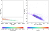 |
Fig. 1 Hertzsprung – Russel diagram of M dwarfs. The left panel shows the relation between the effective temperature (Teff) and the surface gravity (log g). The metal-licity ([Fe/H]) is colored. The right panel shows the relation between the color index (GBP – GRP) and the apparent magnitude (MG). The number of stars is colored. |
Stellar parameters of M dwarf stars from LAMOST DR10.
2.2 TESS light-curve survey
The Transiting Exoplanet Survey Satellite space telescope was launched by NASA and was sent into orbit on April 18, 2018, on board the SpaceX Falcon 9 rocket. In the past five years, TESS has focused on conducting an all-sky survey to discover exoplanets orbiting nearby bright stars (Ricker et al. 2015). The TESS primary mirror consists of four identical cameras, each containing seven lenses, a set of detectors, and electronic components, with a lens sunshield. The combined field of view of the four cameras is 24° × 96°, and the survey can observe stars up to magnitude 13 (V <13) (Kossakowski et al. 2019). TESS possesses the observational capability to detect solid terrestrial planets and giant gas planets in potential orbits, effectively addressing the limitations of ground-based telescopes. Currently, TESS is observing 83 sectors located in orbit 174 and has successfully collected over 1.3 million light curves with 2-minute cadences. By conducting a detailed analysis of these light curves, we can more accurately trace dynamic changes in stellar surface activity, thereby uncovering potential connections between stellar magnetic activity and surface phenomena. Through crossmatching M dwarf samples with TESS observation sectors, we obtained light curves for 2868 M dwarfs, which provides a valuable dataset for studying the physical characteristics and activity behaviors of these stars. These light-curve data enabled us to conduct an in-depth investigation of the variability amplitude, periodicity, and potential starspot characteristics of M dwarfs. By analyzing the data, we can gain a more comprehensive understanding of the rotational periods, magnetic activity cycles, and the ways in which these properties evolve with stellar Teff and mass.
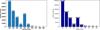 |
Fig. 2 Distribution statistics of the number of stars and spectra for each subclass. Left: bar chart showing the distribution of the number of stars in each subclass. Right: bar chart showing the distribution of the number of spectra for each subclass. |
3 Results and discussion of the stellar chromospheric activity
3.1 Stellar magnetic activity indicator: The Hα spectral line
Reiners & Basri (2008) established the magnetic activity threshold distinguishing inactive from active stars through an analysis of the Hα emission line widths in late-type dwarfs. They systematically revealed a significant correlation between the activity levels and stellar rotation rates. Newton et al. (2017) extended these studies by systematically mapping the evolution of the magnetic activity with age in young stellar populations through measuring the Hα line width. They revealed an activity saturation. Long et al. (2021) used the EWHα to establish empirical relations between stellar activity levels (characterized by the EW) and fundamental parameters (e.g., mass and metal-licity) through large-sample statistics. These studies not only established the methodological foundation of Hα spectroscopic diagnostics for stellar magnetic activity, but more importantly, they revealed intrinsic connections between the activity strength and fundamental stellar parameters (e.g., rotation, age, and mass). Similarly, our investigation examines stellar magnetic activity through atomic line emission. By using EWHα measurements, we systematically tested activity-parameter correlations. We applied the methods from Hawley et al. (2002) and West et al. (2004) to calculate the EW of the stellar spectrum as follows:
 (1)
(1)
where Fλ is the line flux of the spectral line in the stellar spectrum, and Fc is the flux of the continuum at the two ends of the spectral line. West et al. (2004) calculated EWHα using the trapezoidal integration method to sum the flux under the emission line. To determine the continuum flux Fc, they took the Hα line center as a reference and selected spectrum ranges of 50 Å on either side: 6500-6550 Å for the left side, and 6575-6625 Å for the right side. This method is suitable for calculating continuum flux in low-resolution spectra, but for medium-resolution spectrum, its application in quantifying the Hα line may have certain limitations. Therefore, we used a shorter continuum flux range at both ends of the line. Medium-resolution spectra provide finer detail than low-resolution spectra, and we therefore selected narrower spectral sections to avoid contamination from the continuum. This adjustment ensured the accuracy of the measurements, especially in the complex background around the Hα line. The spectrum ranges we used (6500-6525 and 6610-6635 Å) are narrower than those in low-resolution spectra, which helped us to improve the quantitative accuracy of medium-resolution spectrum. Additionally, we adjusted the line width of the Hα emission line to 15 Å (6555.85-6570.85 Å), which is slightly broader than the 14 Å used by West et al. (2004) and the 10 Å adopted by Han et al. (2023), which is an optimization based on the requirements of medium-resolution spectrum. This approach was taken to capture the shape of the emission line more accurately and to maximize the detection of subtle features in the wings of the Hα line. Compared to low-resolution spectra, medium-resolution spectrum allow for a more detailed analysis of the line profile and thus provide a higher-precision when the EWHα is measured. We list the EWHα values for each star in Table 2. We plot the relation between Teff and EWHα for the sample in Figure 3. An EWHα value of 0.75 was considered the baseline for Hα line emission and was taken as the reference for M dwarf chromospheric emission. Figure 3 shows decreasing EWHα values of stars with rising effective temperature, although this declining trend becomes less pronounced at Teff > 3600 K. We performed a temperature-binned analysis by dividing the sample into several Teff intervals and calculating the median EWHα in each bin (red line). The results indicate that for stars with Teff > 3600 K, EWHα remains relatively stable and shows no significant trend with increasing temperature. In contrast, for Teff ≤ 3600 K, the EWHα values exhibit a larger scatter and display a gradual decrease as Teff increases. This trend indicates that the stellar activity gradually weakens with increasing temperature, which might be attributed to reduced chromospheric activity in higher-temperature M dwarfs. As Teff increases, the EWHα value gradually approaches or falls below 0.75, indicating that chromospheric activity is more significantly suppressed at higher temperatures. This aligns with our understanding of M dwarfs, where lower-temperature M dwarfs typically exhibit more active chromospheric activity. Figure 4 illustrates the differences in chromospheric activity among M dwarfs of various spectral types. The proportion of active stars increases with later spectral types, which further confirms that lower-temperature M dwarfs typically exhibit a higher chromospheric activity.
Magnetic activity occurs frequently in late-type stars, which makes it a significant aspect of study. Therefore, we focus on the chromospheric activity of M dwarfs. The molecular band structure is prominent in M dwarfs, and it is therefore challenging to directly obtain their true continuum. As a result, we adopted the standard proposed by Hawley et al. (2002) to assess the activity of M dwarfs. The criteria were as follows: 1. EWHα > 0.75. 2. The EWHα value must be greater than three times the standard deviation, that is, EWHα > 3σ. 3. The emission strength of the Hα line must be greater than three times the noise level at the line center. We identified 1676 M dwarfs in the 11 868 M dwarf stars with emission features, and the signal-to-noise ratio of these samples was greater than 10. The measurement data of our sample are listed in Table 2, which also includes parameters such as stellar rotation period, signal-to-noise ratio, spectral type, and stellar activity.
Stellar parameters of M dwarf stars obtained through calculation and cross-matching.
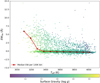 |
Fig. 3 Relation between Teff and EWHα. The stellar surface gravity is colored. Teff was obtained from cross-matching the TESS input catalog v8.2 using TOPCAT (Taylor 2020). The red line divides the stars into effective temperature intervals, indicating the median EWHα within each interval. |
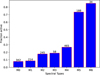 |
Fig. 4 Distribution of activity proportions for M dwarfs of different subtypes. The data labels represent the number of active stars. |
3.2 Hα line variation
Stellar magnetic activity variations are often studied by analyzing changes in the Hα spectral line. Kruse et al. (2010) investigated variations in the EWHα values of the Hα line to explore the evolution of stellar magnetic activity in multiple observations. Lee et al. (2010) and Kruse et al. (2010) used REW (REW=EWmax/EWmin) to quantify the variations in the Hα line and concluded that the later the spectral type of the star, the greater the amplitude of the Hα line variations. We calculated the coefficient of the variation (C.V.) for EWHα (the C.V. is defined as the ratio of the standard deviation to the mean of the EWHα values for each star. It simultaneously captures variations in dispersion and central tendency (C.V. = σ/μ × 100%)) in the sample and statistically distributed the quantities of each C.V., as shown in Figure 5. The left panel shows the bar chart of the distribution of exposure counts for each star. The right panel illustrates the distribution of the EWHα variation coefficients (C.V.) for the sample stars, where the number of stars decreases gradually as the coefficient increases. The variations in the EWHα values for individual stars are plotted in Figure 6. The left panel presents the statistical distribution of δEWHα (EWHα) for individual stars. The δEWHα variation coefficients of most stars are concentrated between 0.1 and 0.2. Beyond a δEWHα value of 0.1, the number of stars decreases as the variation coefficient increases. The right panel quantifies the variations in EWHα using REW, and the black line represents the median REW for each spectral subtype. The figure shows that the variability in the Hα line increases as the spectral type progresses to later types. This is consistent with the research findings of Bell et al. (2012) and Lee et al. (2010).
Gizis et al. (2002) used EWHα to study the variations in stellar magnetic activity during repeated observations and found that as the standard deviation of EWHα (σEWHα) increased, the EWHα value also increased. We calculated the EWHα values in the sample, along with their corresponding standard deviations (σEWHα) and the ratio (σEWHα/EWHα), and we examined the relations between them, as shown in Figure 7. The relation between EWHα and its standard deviation (σEWHα), as well as the ratio of EWHα to its standard deviation (σEW/<EW>), is shown in the figure. The red line reflects the trends and distribution characteristics of these variables, with results consistent with Gizis et al. (2002)'s study. We also present the spectral diagram of Hα line variations and the EWHα variation plot on short timescales, as shown in Figure 8. In the left panel, the spectral diagram clearly shows the variation in the Hα line. In the right panel, the dynamic evolution of EWHα on short timescales is presented. This variation plot clearly shows the fluctuations in the values of EWHα over time, along with the corresponding changes in the associated features.
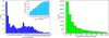 |
Fig. 5 Left: bar chart showing the distribution of the stellar exposure counts. The x-axis label refers to the binned ranges of exposure counts per star. Right: bar chart displaying the statistics of the variability coefficients for stars. |
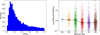 |
Fig. 6 Equivalent width (EW) of the Hα line variation statistics. The left panel shows the distribution statistics of δEWHα ( |

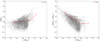 |
Fig. 7 Relation between EWHα, its standard deviation (σ EWHα), and the ratio of the standard deviation to EWHα is as follows (σEWHα/<EWHα>): The left panel illustrates the relation between EWHα and σEWHα, and the right panel shows the relation between EWHα and σEWHα/<EWHα>. The red line represents the median value within each interval. |
3.3 Stellar chromospheric activity index R′Hα
The study of the stellar chromospheric activity is typically closely related to the stellar temperature and spectral characteristics. Figure 3 shows the significant correlation between the EWHα and the effective temperature. In general, stars with lower temperatures tend to exhibit a stronger continuity in their magnetic activity. Under the condition of consistent activity levels, the EWHα value is therefore expected to be higher. A more effective approach to analyzing stellar magnetic activity is to introduce a quantity that is independent of the stellar temperature and spectral type, however, namely R′Hα. R′Hα is defined as the ratio of the line luminosity (LHα) in a stellar spectrum to its total bolometric luminosity (Lbol) (Walkowicz et al. 2004; Frasca et al. 2016). This ratio helps us to quantify the level of magnetic activity in the star, with higher values indicating stronger magnetic phenomena. Additionally, (Walkowicz et al. 2004) introduced the χ factor, which is independent of the stellar distance. The χ factor is a normalized parameter that describes the relation between a specific wavelength of the star (e.g., near the Hα line) and its total radiation. It represents the ratio of the stellar surface continuous spectrum radiation flux near the Hα line (FHα) to the total stellar radiation flux (the flux across all wavelengths, referred to as bolometric flux, or Fbol). This is expressed by the following formula:
 (2)
(2)
In the formula, σ represents the Stefan-Boltzmann constant, and Teff is the effective temperature of the star. The χ factor normalizes the radiation flux near the Hα line (FHα) by comparing it to the total stellar radiation flux (Fbol), effectively eliminating the influence of distance. This facilitates a comparison and study of the stars at different distances. The χ factor is particularly useful to study the stellar luminosity, temperature, and other characteristics, especially when a spectral analysis across different wavelengths is considered. When the stellar chromospheric activity indicator R′Hα is calculated, the distance-independent χ factor is therefore introduced to compute the ratio (L′Hα/Lbol), as shown in the following formula (Walkowicz et al. 2004):
 (3)
(3)
The use of the R′Hα chromospheric activity indicator effectively eliminates variations in the continuous flux within specific regions of a stellar spectrum, which enables a better comparison of the stellar activity levels for dwarfs of different spectral types. This approach provides a reliable tool for studying the chromospheric activity features of various dwarf stars, reveals their behavioral differences under different environmental conditions, and offers essential data for the development of stellar evolution models. The calculated R′Hα values are listed in Table 2, and the distribution of R′Hα values for each star is shown in Figure 9. As shown, the log R′Hα values of the stars are generally in the range of −4.5 to −3.5. The distribution of R′Hα values and the distri bution of active stars reported by West et al. (2004) and Newton et al. (2017) are broadly consistent with that of the active stars in our sample, which have R′Hα values around ≈3.5. West et al. (2004) reported that the log R′Hα values were mainly distributed in the range of −3 to −5, with active stars concentrated around log R′Hα ≈ −4. Newton et al. (2017) reported a distribution ranging from log R′Hα = −3 to −6, where the active stars also cluster around log R′Hα ≈ −4. The double-Gaussian fit reveals two peak values at approximately −4.2 and −3.6 along the x-axis. This distribution may be influenced by factors such as the strength of the stellar magnetic activity and whether the stars exhibit flaring behavior.
3.4 The relation between chromospheric activity and stellar rotation
The factors that affect the strength of a stellar magnetic field include the depth of the convection zone, the effect of Coriolis forces, and the shear forces resulting from differential rotation. For hot stars, the heating mechanisms in the chromosphere and transition region are likely caused by acoustic-wave damping, whereas for cool stars, magnetic effects dominate. The transition in heating mechanisms between hot and cool stars occurs around the F5 spectral type (Simon & Drake 1989; Brito & Lopes 2019). Walter (1983) found that for stars near the F5 spectral type, the relation between rotation and activity begins to emerge, which suggests that magnetic generation mechanisms similar to those of the Sun start to form.
Babcock (1961) used the α-Ω dynamo model to further investigate the relation between chromospheric activity, stellar rotation, and convection. This model is widely used to explain magnetic activity in late-type stars. Magnetic activity in late-type stars is typically triggered by differential rotation at different latitudes and by radial spiral effects (Mohanty & Basri 2003). This study also introduced the Rossby number (Ro) to analyze the relation between chromospheric activity and stellar rotation and convection (Noyes et al. 1984; Mamajek & Hillenbrand 2008). The Rossby number is defined as the ratio of the stellar rotational period (Prot) to the convective turnover time (τ), and it is expressed as Ro = Prot/τ. To more precisely investigate the relation between chromospheric activity intensity and the Rossby number, samples of binary stars from the VSX catalog and the TESS binary star catalog were excluded from the study (Watson et al. 2006; Green et al. 2023). By combining the TESS periodic star catalog and the VSX catalog, the rotation periods of the sample stars were determined, and the Lomb-Scargle (Lomb 1976; Scargle 1982; Fetherolf et al. 2023) method was applied to calculate the periods of 598 stars and identified whose periods were within the 10% error of the previous. Considering the limitations of TESS observations, we selected stellar samples with rotation periods ≥20 days and replaced them with the most reliable periods from McQuillan et al. (2013) and Sousa et al. (2019), among others. The TESS observations confirm a significant dependence on spectral type in the magnetic activity of early- to mid-M dwarfs. As demonstrated by Stelzer et al. (2022a) in their analysis of 112 M dwarfs, the reliable detection rate for the rotation period of M 4-M 5 type stars (≈ 11%), though lower than in the Kepler sample, shows that its flare rate peaks at M 3-M 4 spectral types. This finding, combined with the X1445 class superflare observed on AD Leo (M3.5) by Stelzer et al. (2022b), indicates that rapidly rotating early-M dwarfs remain significant sources of high-energy radiation. The calculation of τ was based on the empirical formula proposed by Wright et al. (2018), which correlates τ with stellar mass. The formula is as follows:
 (4)
(4)
In the formula, M represents the stellar mass. The stellar masses M was obtained from the TESS input catalog v8.2 (Stassun et al. 2019) by cross-matching using TOPCAT (Taylor 2020) with a matching radius of 2 arcseconds to identify the corresponding stars. The masses of late-type stars (M type and late-K type) were are further corrected based on the empirical MKS -M* relation established by Mann et al. (2019) from 62 nearby binary systems, which achieves an accuracy of 2-3% in the range of 0.075-0.70 M⊙. The calculated values of Ro and the τ are listed in Table 2. Subsequently, the correlation between Ro and the chromospheric activity index R′Hα was analyzed, as shown in Figure 10. The horizontal axis represents Ro, and the vertical axis represents R′Hα. The red and blue lines in the figure are the fit line of the sample, and this fit line was obtained according to the following formulas (Douglas et al. 2014; Newton et al. 2017):
 (5)
(5)
In the fitting procedure shown in Figure 10, we employed a piecewise regression method. First, we restricted the candidate saturation point range to [0.08,0.4] to ensure that the slope of the fit tended toward zero in the leading segment and approached its most negative value in the trailing segment. This range was then discretized into 100 points, and linear fits were iteratively performed for each candidate saturation point, and we calculated the corresponding fit error. The point yielding the smallest error was chosen as the final saturation point. As shown Figure 10, the Rosat value displays a distinct decrease in slope at Rosat = 0.18 ± 0.03. This phenomenon is associated with the critical point between saturated and unsaturated stellar activity. This critical point remains a topic of debate, however. For example, Douglas et al. (2014) reported a Rosat value of 0.11 ± 0.02, while Newton et al. (2017) found a value of 0.21 ± 0.02, Fang et al. (2018) determined the critical Rosat value to be 0.25, and Zhang et al. (2023) identified it as 0.12. The variation in the slope of the activity index and the threshold value of the Rossby number is attributed to differences in the sample selection, analytical methods, and the treatment of activity indicators in these studies. For our sample, the Rosat value was 0.18 ± 0.03, and the slope of the decrease in the unsaturated phase was −0.77 ± 0.01. The slope value is consistent with the error range reported by Douglas et al. (2014), which confirms that chromospheric activity in late-type stars systematically decreases with increasing Rossby number in the unsaturated regime.
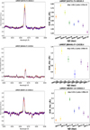 |
Fig. 8 Hα variation in the selected examples. The left panel shows the spectrum that clearly displays the changes in the Hα line. The right panel visually presents the dynamic evolution of EWHα on short timescales, and the vertical red lines indicate the error bars. The colors of the spectral profiles in the left panel correspond to the points in the right panel, which are labeled with their respective heliocentric Julian dates, which allow a clear identification of the observation epochs. |
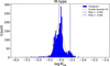 |
Fig. 9 Distribution histogram of a double-Gaussian fit of the R′Hα value. The x-axis represents the R′Hα values of each star, and the y -axis represents the number of stars. |
 |
Fig. 10 Correlation between chromospheric activity indicators R′Hα and the Rossby number (Ro). The red and blue lines show the fit relation between these parameters. The color represents the stellar Teff. |
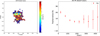 |
Fig. 11 Two-dimensional and one-dimensional distribution of active stars based on the Hα line. The left panel illustrates the two-dimensional distribution of the ratio of active stars to the total number of stars in cylindrical galactocentric coordinates (R and Z), where the color indicates the active fraction. The right panel shows the relation between stellar activity proportions and the vertical distance from the Milky Way plane. The vertical red lines represent the error bars. |
3.5 Chromospheric activity distribution of M dwarfs in the Milky Way
Pineda et al. (2013) confirmed that the proportion of stellar activity decreases with increasing distance from the Galactic plane, and they explained this phenomenon as a consequence of the vertical age gradient of stars. We plot the distribution of the stellar activity proportions within the Milky Way for the sample in Figure 11. The left panel shows the spatial distribution of stellar activity proportions in the Milky Way, where R represents the distance from the projected point of the star on the Milky Way plane to the Milky Way center, and Z represents the vertical distance of the star from the Milky Way plane. The distribution of M dwarfs in the galaxy appears to be radial, with colors representing the activity proportions of the stars. The right panel shows the relation between stellar activity proportions and the vertical distance from the Milky Way plane. The results indicate that as the vertical distance from the Milky Way plane increases, the stellar activity proportion gradually decreases. This confirms the distribution of stellar activity in the Milky Way.
4 Stellar flares and starspots
Stellar flares are sudden intense energy releases on the surface of stars, where a large amount of energy is emitted in a short period. This causes a rapid increase in brightness. The shpae of the light curve is characterized by a fast rise and slow decay. Currently, astronomy is entering an era of long-term photometric monitoring, which provides a wealth of data and fosters the study of stellar flare characteristics (e.g., energy, frequency, amplitude, and duration). We used TESS light curves to search for flare events in the sample, systematically identified flare events in the TESS data, and calculated the flare energy and frequency for each event. Through a statistical analysis of these flare events, we plot the relation between flare energy and frequency, and compared the flare characteristics of different stellar types.
4.1 Search for stellar flares
Stellar flares are usually closely related to magnetic reconnection events. Magnetic reconnection is the process in which magnetic field lines reconnect and release a large amount of energy, either within a stellar interior or in its atmosphere. This process can lead to an intense energy release, resulting in flare phenomena. The intensity and frequency of flare events are typically related to the stellar magnetic activity and internal structure. Therefore, studying the mechanism of magnetic reconnection is crucial for understanding the origin of stellar flares. Hawley et al. (2014) conducted a detailed analysis of flare activity in M dwarfs using data from the Kepler survey, investigating the relations among flare frequency, energy distribution, and stellar magnetic activity in active and inactive M dwarfs. They found that mid-type M dwarfs (M3-M5) tend to exhibit frequent but low-energy flares. Davenport (2016) explored flare activity in M-type stars using TESS survey data and provided statistical characteristics of flare frequency and energy. They observed that complex multi-peaked events are more common in high-energy flares. Günther et al. (2020) studied M dwarf flares using TESS data and found that these flares can erode exoplanet atmospheres and impact habitability. Their results also confirmed that rapidly rotating M dwarfs have the most flares, and that flare amplitudes are independent of the stellar rotation period. In recent years, two main methods have been used to identify flares. One approach was to examine spectrum lines in raw spectra to spot flare events amidst strong background light curves, followed by detection in the detrended data. Another method involves using neural networks or machine-learning techniques to automatically identify and classify flare features (Feinstein et al. 2020). Both methods have their advantages, and they provide richer tools and approaches for the study of stellar flares. In most studies, the method of fitting background light curves to detect stellar flare events is commonly used (Gao et al. 2016; Lu et al. 2019; Günther et al. 2020). We also used the method of fitting background light curves to identify stellar flare events. By cross-matching our sample with TESS data, we obtained light-curve data for 2,868 stars and identified 891 flare stars. We extracted the SAP (PDC-SAP) flux from the TESS light-curve data to search for flares. By optimizing the S/N, correcting the light-curve background, and removing systematics caused by satellite rotation using the common trend basis vectors, we calculated the average PDCSAP flux for each dataset, denoted as Fave, using the following formula:
 (6)
(6)
In this formula, Fmax represents the maximum flux value, and Fmin represents the minimum flux value. Next, the following formula was used to normalize the photometric data (PDCSAP flux):
 (7)
(7)
In the above formula, Fnorm represents the normalized result, where FPDC is the PDCSAP flux. To improve the accuracy of the search results, we removed the variability of background stars from the normalized raw light curves. First, we excluded points in the normalized light curve that deviated by more than three times the standard deviation. Then, the remaining data were split and fit multiple times, and the best fit was selected as the background variability. The specific fitting process was described by Yang et al. (2023). In the dispersion sample of M dwarfs, we identified a total of 3653 flare events from 891 flare stars, and the parameters of these 3653 flare events are listed in Table 3.
Stellar flare parameters of M dwarf stars.
4.2 Flare parameters
We calculated the flare energy of stellar flares using the following formula (Lu et al. 2019):
 (8)
(8)
In this formula, Eflare represents the flare energy of the star, Fflare is the normalized PDCSAP flux, σSB is the Stefan-Boltzmann constant, R is the stellar radius, and T is the effective temperature obtained from the TESS input catalog. The energy is expressed in erg. The calculated flare energy is listed in Table 3. Based on the calculated flare energies, the flare energy range of our sample is comparable to the results of studies by Tu et al. (2021), with an energy range of: 2.15 × 1031 ~ 1.07 × 1036 erg. For the calculated flare energy results, as shown in Figure 12, the left panel shows the relation between the flare energy and the duration for all flare data samples, and the red line represents the fit result. The slope of the fit is 0.29, indicating a positive correlation. The right panel shows the relation between the log of the flare energy and the duration for all samples, and the color bar represents the number of flare events. The energy of most of the flare events lies in the range of 1032−1034 erg.
Subsequently, the subspectral types within the M dwarf sample were distinguished to statistically analyze the relation between the flare energy and the duration across different spectral types. Figure 13 shows the relation between the flare energy and the duration for M dwarf stars of different subtypes. With increasingly later spectral type, the slope of the positive correlation in the fit results decreases gradually. The slopes of the fitting lines for the subspectral types of M dwarf stars were found to range between 0.29 and 0.43, indicating that the duration t ∝ E0.29−0.43. This result can be explained by magnetic reconnection theory, which suggests that the power-law index should be close to one-third. These studies confirmed this conclusion partially. For example, Namekata et al. (2017) used solar flare data and derived t ∝ E0.38±0.06. Tu et al. (2021) found that for solar-like stars in their sample, the relation between the flare energy and the duration was t ∝ E0.42±0.01. Figure 14 shows the relation between the log flare energy and the flare duration for M dwarf stars of different spectral subtypes. The longer the flare duration, the higher the flare energy. The color bar on the right represents the number of flare events. The figure also shows that for M dwarfs of different spectral subtypes, flare events with a duration shorter than 60 minutes are more common, while high-energy flare events tend to have longer durations. We also analyzed the relation between the stellar chromospheric activity and stellar starspots. To characterize the strength of stellar spot activity, we introduced the parameter Reff (effective spot radius), which is a key derived quantity representing the characteristic scale of starspots. It is defined as the radius of a single circular spot that would produce the observed equivalent photometric modulation amplitude (∆F/F). The calculation of Reff was adapted from the method proposed by He et al. (2015) and He et al. (2018). The core relation we used was
 (9)
(9)
In the formula, frms represents the previously defined fr (García et al. 2010; Chaplin et al. 2011), where fr refers to the relative flux of each star after noise was remed. The coefficient preceding the formula serves as a correction factor, as proposed by He et al. (2015). Based on the TESS light curves and using methods established in previous studies (Zhang et al. 2020b), we calculated the amplitude of the photometric modulation caused by photospheric starspot activity. The left panel in Figure 15 shows the relation between the chromospheric activity indicator, R′Hα, and stellar starspots, and the right panel shows the relation between EWHα and stellar starspots. The fit lines show that the results are positively correlated, which indicates a positive correlation between the stellar chromospheric activity and stellar starspots.
We plot the distribution of the total number of flare durations and flare amplitude in Figure 16, where each subplot is a magnified version of the corresponding section in the main figure. The left panel of Figure 16 shows that the distribution of flare durations tends to decrease, and the highest number of events occur at a duration of 1.5 hours. The right panel shows that the distribution of the flare amplitude decreases as the amplitude increases, and the amplitude of most flare events lies in the range of 0.15.
We calculated the percentage of flare event durations and amplitude in different ranges relative to the total sample, as shown in Figure 17. The left panel shows the distribution of log flare durations, where the logarithm of the duration (log Dur) is primarily concentrated between −0.5 and 0.5, indicating that most flare events last between 10 minutes and 1 hour. The distribution is approximately normal, with a peak around log Dur ≈ −0.2, meaning that these flare events lasted around 40 minutes. The right panel shows the distribution of log flare amplitude, with log Amp concentrated between −2 and −1, indicating that most flare events have relatively small amplitude increases. The peak occurs around log Amp ≈ −1.6, suggesting that the amplitude of most flare events lies in the range of 0.025. Overall, these two charts show the percentage distribution of flare event duration and amplitude in different ranges, revealing that their distributions are close to normal, with distinct peak regions for each. Next, in our study of the Hα line variations, we specifically searched for flare-like changes in the Hα line, including rapid rises and slow decays in the EWHα values. We identified 119 stars with EWHα flare-like events and calculated the energy and amplitude of the EWHα variations for these events (Wu et al. 2022). The energy ranged from 6.12 × 1028 to 3.05 × 1035 erg. The specific steps for calculating the EWHα energy were based on Wu et al. (2022), and the results are listed in Table 2. Several clear representative examples were selected to illustrate typical EWHα flare-like events observed in our sample. The EWHα variation diagrams of these events are presented in Figure 18, showing changes in Hα on short timescales. This figure shows the changes in the EWHα energy and amplitude on this timescale, and it reveals a trend of a rapid rise and slow decay in the EWHα values. Twenty-five of the 119 stars with EWHα flare-like variations were flare stars.
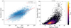 |
Fig. 12 Relation between stellar flare energy and duration. The left panel shows the relation between the flare energy and the duration for all flare data samples. The red line represents the fit result. The right panel shows the relation between Log(flare energy) and the duration for all samples. The color bar represents the number of flare events. |
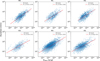 |
Fig. 13 Relation between flare energy and duration for M dwarf stars of different subtypes. |
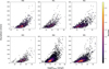 |
Fig. 14 Relation between the log flare energy and the flare duration for M dwarf stars of different spectral subtypes. |
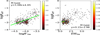 |
Fig. 15 Left panel: relation between the chromospheric activity indicator R′Hα and stellar starspots. Right panel: relation between EWHα and stellar starspots. |
4.3 Hα asymmetry
A stellar flare is a violent release of energy from the stellar surface that typically converts magnetic energy in the corona into kinetic and thermal energy through magnetic reconnection. It is often accompanied by CMEs. Stellar flares and CMEs can affect the magnetic field and ionosphere of a planet and might erode or strip away the planetary atmosphere, thereby affecting the habitability of the planet (Shibata & Magara 2011; Temmer 2021; Cliver et al. 2022). Observations of stellar optical spectra can provide important indications of stellar CMEs. Currently, the detection of stellar CMEs mainly relies on the Doppler-shift method, which identifies them through the emission or absorption enhancements in spectrum lines. Namekata et al. (2022) investigated the superflare on the young Sun-like star EK Dra through detecting the Hα spectrum. The blueshifted absorption observed in the Hα spectrum is considered evidence of a massive stellar filament eruption. Lu et al. (2022) identified three stellar CME candidates by examining the asymmetry of the Hα spectral profiles. Wang et al. (2024) and Xu et al. (2025) also confirmed two objects with an Hα asymmetry by analyzing the symmetry of their Hα spectral profiles. We used the Doppler-shift method to search for potential stellar CMEs in the LAMOST sample of dispersed M dwarf stars. In the search for stellar CMEs, we identified them by inspecting the asymmetry of the Hα spectrum lines in LAMOST medium-resolution spectra. There are various methods to determine the asymmetry of spectral profiles (Maehara et al. 2021 ; Koller et al. 2021). We quantified the asymmetry of the Hα spectral line by calculating the difference in the integrated areas on either side of the Hα profile peak. We normalized the LAMOST medium-resolution spectrum using the average flux of the spectrum as the reference, as shown by the baseline (horizontal black line) in Figure 19. The dashed red and green lines represent the integration boundaries, and the dashed yellow and blue lines indicate the theoretical and actual peak values of the Hα profile. To determine whether the Hα spectral line shows a redshift or a blueshift, we plot medium-resolution Hα spectrum for individual spectra. By calculating the peak flux ratio (0.2, 0.4, 0.6, and 0.8), which represents the fraction of the spectral flux above the baseline, after subtracting it from the peak, we analyzed the differences in the line profile distribution between the two sides. when the average difference between the two sides exceeded 0.56 Å (with an error of 0.14 Å per region), a redshift or blueshift was identified. We simultaneously examined all spectra and cross-matched them with the SIMBAD database (Wenger et al. 2000), excluding pulsating variables such as eclipsing binaries, T Tauri stars, and RR Lyrae stars, which might affect the Hα spectrum lines. We identified 289 medium-resolution Hα spectra with blueshifts or redshifts, from which we identified two objects with Hα asymmetry features.
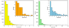 |
Fig. 16 Number distribution of the stellar flare duration and flare amplitude. The left panel shows the number distribution of stellar flare durations, and the right panel shows the number distribution of the flare amplitude. |
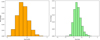 |
Fig. 17 Percentage distribution of the flare event duration and amplitude in different ranges relative to the total sample. The left panel shows the distribution of the flare duration percentages, and the right panel shows the distribution of the flare amplitude percentages. |
4.4 Stellar CME candidates
To identify CME candidates, we searched for potential CME candidates by detecting red- or blueshifted asymmetries in spectral stellar Hα lines. In 289 objects with red- or blueshifted spectrum lines, the Hα asymmetry sample was identified through visual inspection. Using the methods described above and through manual inspection of the identified candidates, we ultimately confirmed two stars as CME candidates. CME candidate 1 is an M2-type main-sequence star (LAMOST J133213.26+505702.2), which is also the flare star TIC 320351354. The LAMOST medium-resolution spectrum of this star consists of three consecutively observed subspectra. Figure 20 displays the stellar spectra, with the left panel showing the three preprocessed Hα spectra, and the middle panel showing the smoothed Hα spectra. The first two spectra (blue and orange lines) are slightly asymmetrical, with minor variations in the intensity of the Hα emission. They are largely consistent with each other, however, which indicates that the Hα emission in these two spectra remains relatively stationary with respect to the stellar system. We therefore used the first spectra as reference spectra. The third spectrum (green line) shows a clear enhancement of the red wing and asymmetry, representing the active spectrum. We compared the active spectrum with the reference spectrum using a double-Gaussian fit, and the fit results are shown in the right panel. This method refers to the work of Lu et al. (2022), with the vacuum wavelength data of the Hα spectral line obtained from van Hoof (2018). From the fit contrast profiles, the dashed blue and red lines exhibit redshift components. This phenomenon is likely caused by chromospheric condensation or coronal rain (Canfield et al. 1990; Lu et al. 2022; Cao et al. 2023). Coronal rain is the phenomenon in which condensed plasma in the corona of the Sun or a star falls back from higher atmospheric layers to lower ones (e.g., the chromosphere) along magnetic field lines under the influence of gravity. Because this process looks like falling rain, it is called “coronal rain”. We calculated the radial velocity of the third spectrum to be 76.38 km/s. This velocity falls within the typical range of coronal rain velocities (30-150 km/s) (Oliver et al. 2016; Lu et al. 2022), and we therefore conclude that coronal rain is the primary cause of this phenomenon. After cross-analyzing TESS data, we obtained the light curve of the star. Stellar flares were clearly identified in the light-curve data. The cooling phase following these flare events might be one of the factors that contribute to the redshift observed in the Hα spectral line. During the cooling phase following a flare, some plasma becomes thermally unstable, condenses, and falls toward the lower atmosphere along magnetic field lines, forming coronal rain. The lower panel of Figure 20 illustrates the identified flare events in the stellar light curve, along with a magnified view of the corresponding flare regions.
The CME candidate 2 (LAMOST J030002.90+550653.0) was identified as a high proper motion star through crossmatching with the SIMBAD database. A flare event for this star was also detected in the TESS light-curve data (TIC 251469806). The LAMOST medium-resolution spectrum of this star consists of four consecutively observed subspectra. Figure 21 shows the spectrum of this star. The first and second of these Hα spectra (blue and orange lines) have similar shapes and emission strengths for the Hα line, and thereby, we considered them as reference spectra. In contrast, the third and fourth spectra (green and red lines) clearly show an increase in the Hα line emission strength, asymmetry in the line, and a blueshift. Therefore, we considered these two spectra as active spectra. After we performed a double-Gaussian fit on the contrast spectrum profile (see the right panel of Figure 21), the fitting results revealed a blueshifted (red line) component and a broad emission component (blue line) centered around other wavelengths of the Hα line. The radial velocity of its active spectrum is 71.61 km/s. The blueshifted component in the Hα line profile might originate from CME eruptions along the line of sight, while the broad emission component (blue line) in the double-Gaussian fit might be related to Stark broadening caused by electron acceleration (Muheki et al. 2020; Wu et al. 2022). By crossmatching with TESS data, we obtained the stellar light curve, which revealed flare events through analysis. We suggest that the blueshift observed in the Hα spectral line might be associated with a CME that accompanied the stellar flares.
Although we identified two CME candidate events based on asymmetries in the Hα line, spectral features alone are not sufficient to confirm the existence of CMEs. To further verify these candidates, we searched the 3XMM-DR5 catalog (He et al. 2019) and the study by Wang et al. (2020) on X-ray activity, but found no corresponding X-ray observations for the two stars. The lack of simultaneous X-ray and TESS observations prevents us from providing additional supporting evidence. At present, multiwavelength coordinated observations of M dwarfs remain challenging. In the future, combined monitoring with optical, X-ray, and space-based photometric data may help us to improve the reliability of a CME identification.
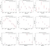 |
Fig. 18 Dynamic evolution of the EWHα on short timescales. The values of the EWHα energy and amplitude changes are shown, and the vertical red lines indicate the error bars. |
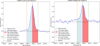 |
Fig. 19 Examples of the Hα profile asymmetry in stellar redshift and blueshift integration regions for CME detection. Left: LAMOST J133213.26+505702.2. Right: LAMOST J030002.90+550653.0. The dashed red and green lines represent the integration boundaries, the dashed yellow and blue lines indicate the theoretical and actual peak positions of the Hα profile, and the light blue and red regions represent the integration areas. |
5 Summary
We used the TESS light-curve data of 2868 M dwarfs and 20 279 stars from the LAMOST MRS DR10 to investigate stellar chromospheric activity and flare events. The chromospheric activity was determined based on the EWHα and the R′Hα index to assess the stellar chromospheric activity. The EWHα values were calculated for 16 504 M dwarfs, 11 868 of which had a signal-to-noise ratio greater than 10, and 1676 of these M dwarfs were identified as active stars. The distribution of the stellar activity by spectral subtype showed that the activity ratio increased with later spectral types. A sudden rise in activity was observed between M4 and M5, which was attributed to the fact that stars of spectral types M4 and later are fully convective, whereas earlier types are not. By using the chromospheric activity indicator, R′Hα, and combining it with Ro, we minimized the effects of continuous flux variations specific to the stellar spectral regions, which allowed us to study the stellar magnetic activity more accurately. Based on the correlation between Ro and R′Hα , we conclude that at Rosat = 0.18 ± 0.03, the stars in this sample reach the critical point between saturated and unsaturated phases. The slope of the decline in the unsaturated phase is −0.56 ± 0.07. By combining the Gaia data, we clarified the spatial distribution of M dwarfs in the Milky Way and studied the distribution of stellar magnetic activity. M dwarfs display a radial distribution in the galaxy, with a higher proportion of active stars in regions closer to the Milky Way plane. In the one-dimensional z-axis image, we observed that the proportion of active stars decreases as the vertical distance from the Milky Way plane increases.
Using TESS data, we further investigated stellar flare events. By searching for flare events in the TESS light curves of 2868 stars, we identified 7496 flare events from 891 stars and calculated their flare energies, with an energy range from 2.15 × 1031 to 1.51 × 1036 erg. The results showed that the stellar chromospheric activity is positively correlated with stellar starspots, and the longer the flare duration, the higher the flare energy. By studying the Hα line variations, we found an EWHα-like flare behavior in 119 M dwarfs and calculated the energy variation of EWHα on short timescales, with an energy range from 6.12 × 1028 to 3.05 × 1035 erg. Twenty-five of these 119 M dwarfs showed flare events.
We searched for stellar CMEs based on the asymmetry features of the Hα spectrum lines. Two of the 289 mediumresolution Hα spectra with blue- or redshifted components showed a notable Hα asmmetry. We classified them as CME candidates.
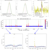 |
Fig. 20 Spectral analysis of the stellar Hα lines and double-Gaussian fit. The left panel shows the preprocessed Hα spectra of the star, the middle panel presents the smoothed Hα spectra, and the right panel displays the contrast flux profile derived from the double-Gaussian fit. The lower panel illustrates the identified flare events in the stellar light curve along with a magnified view of the corresponding flare regions. |
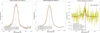 |
Fig. 21 Spectral analysis of the stellar Hα lines and double-Gaussian fit. The left panel shows the preprocessed Hα spectra of the star, the middle panel presents the smoothed Hα spectra, and the right panel displays the contrast flux profile derived from the double-Gaussian fit. |
Data availability
Full Tables 1, 2, and 3 are only available at the CDS via https://cdsarc.cds.unistra.fr/viz-bin/cat/J/A+A/704/A274.
Acknowledgements
This research has been supported by the National Natural Science Foundation of China (NSFC) under Grant Nos. 12373032 and 11963002. Additionally, we acknowledge the use of data from the LAMOST survey, a National Major Scientific Project of the Chinese Academy of Sciences. The paper was also supported by Guizhou Provincial Major Scientific and Technological Program Nos. XKBF (2025) 010 and XKBF (2025)011.
References
- Babcock, H. W. 1961, ApJ, 133, 572 [Google Scholar]
- Brito, A., & Lopes, I. 2019, MNRAS, 488, 1558 [NASA ADS] [CrossRef] [Google Scholar]
- Bell, K. J., Hilton, E. J., Davenport, J. R. A., et al. 2012, PASP, 124, 911, 14 [Google Scholar]
- Canfield, R. C., Penn, M. J., Wulser, J.-P., et al. 1990, ApJ, 363, 318 [NASA ADS] [CrossRef] [Google Scholar]
- Cao, D., Gu, S., Wolter, U., et al. 2023, MNRAS, 523, 4146 [NASA ADS] [CrossRef] [Google Scholar]
- Chang, H.-Y., Song, Y.-H., Luo, A.-L., et al. 2017, ApJ, 834, 92 [NASA ADS] [CrossRef] [Google Scholar]
- Cliver, E. W., Schrijver, C. J., Shibata, K., et al. 2022, LRSP, 19, 2 [NASA ADS] [Google Scholar]
- Chaplin, W. J., Bedding, T. R., Bonanno, A., et al. 2011, ApJ, 732, L5 [Google Scholar]
- Douglas, S. T., Agüeros, M. A., Covey, K. R., et al. 2014, ApJ, 795, 161 [NASA ADS] [CrossRef] [Google Scholar]
- Du, B., Luo, A.-L., Zhang, S., et al. 2021, RAA, 21, 202 [Google Scholar]
- Davenport, J. R. A. 2016, ApJ, 829, 1, 23 [Google Scholar]
- Fang, X.-S., Zhao, G., Zhao, J.-K., et al. 2018, MNRAS, 476, 908 [NASA ADS] [CrossRef] [Google Scholar]
- Feinstein, A. D., Montet, B. T., Ansdell, M., et al. 2020, AJ, 160, 219 [Google Scholar]
- Fetherolf, T., Pepper, J., Simpson, E., et al. 2023, ApJS, 268, 4 [NASA ADS] [CrossRef] [Google Scholar]
- Frasca, A., Molenda-Zakowicz, J., De Cat, P., et al. 2016, A&A, 594, A39 [CrossRef] [EDP Sciences] [Google Scholar]
- Günther, M. N., Zhan, Z., Seager, S., et al. 2020, AJ, 159, 60 [Google Scholar]
- Gaia Collaboration (Vallenari, A., et al.) 2023, A&A, 674, A1 [NASA ADS] [CrossRef] [EDP Sciences] [Google Scholar]
- Gao, Q., Xin, Y., Liu, J.-F., et al. 2016, VizieR Online Data Catalog: J/ApJS/224/37 [Google Scholar]
- García Soto, A., Newton, E. R., Douglas, S. T., et al. 2023, AJ, 165, 192 [CrossRef] [Google Scholar]
- García, R. A., Mathur, S., Salabert, D., et al. 2010, Science, 329, 1032 [Google Scholar]
- Gizis, J. E., Reid, I. N., & Hawley, S. L. 2002, AJ, 123, 3356 [Google Scholar]
- Green, M. J., Maoz, D., Mazeh, T., et al. 2023, VizieR Online Data Catalog: J/MNRAS/522/29 [Google Scholar]
- Han, H., Wang, S., Bai, Y., et al. 2023, ApJS, 264, 12 [NASA ADS] [CrossRef] [Google Scholar]
- Hawley, S. L., Covey, K. R., Knapp, G. R., et al. 2002, AJ, 123, 3409 [NASA ADS] [CrossRef] [Google Scholar]
- Hawley, S. L., Davenport, J. R. A., Kowalski, A. F., et al. 2014, ApJ, 797, 121 [Google Scholar]
- He, H., Wang, H., & Yun, D. 2015, ApJS, 221, 18 [Google Scholar]
- He, H., Wang, H., Zhang, M., et al. 2018, ApJS, 236, 7 [Google Scholar]
- He, L., Wang, S., Xu, X.-J., et al. 2019, RAA, 19, 098 [Google Scholar]
- Kossakowski, D., Espinoza, N., Brahm, R., et al. 2019, MNRAS, 490, 1094 [NASA ADS] [CrossRef] [Google Scholar]
- Kruse, E. A., Berger, E., Knapp, G. R., et al. 2010, ApJ, 722, 1352 [Google Scholar]
- Koller, F., Leitzinger, M., Temmer, M., et al. 2021, A&A, 646, A34 [NASA ADS] [CrossRef] [EDP Sciences] [Google Scholar]
- Laughlin, G., Bodenheimer, P., & Adams, F. C. 1997, ApJ, 482, 420 [NASA ADS] [CrossRef] [Google Scholar]
- Lee, K.-G., Berger, E., & Knapp, G. R. 2010, ApJ, 708, 1482 [Google Scholar]
- Li, J., Liu, C., Zhang, B., et al. 2021, ApJS, 253, 45 [NASA ADS] [CrossRef] [Google Scholar]
- Lomb, N. R. 1976, Ap&SS, 39, 447 [Google Scholar]
- Long, L., Zhang, L.y., Bi, S.-L., et al. 2021, ApJS, 253, 51 [NASA ADS] [CrossRef] [Google Scholar]
- Lu, H.p., Zhang, L.y., Shi, J., et al. 2019, ApJS, 243, 28 [NASA ADS] [CrossRef] [Google Scholar]
- Lu, H.p., Tian, H., Zhang, L.y., et al. 2022, A&A, 663, A140 [NASA ADS] [CrossRef] [EDP Sciences] [Google Scholar]
- Luo, A.-L., Zhang, H.-T., Zhao, Y.-H., et al. 2012, RAA, 12, 1243 [NASA ADS] [Google Scholar]
- Luo, A.-L., Zhao, Y.-H., Zhao, G., et al. 2015, VizieR Online Data Catalog: V/146 [Google Scholar]
- Luo, A.-L., Zhao, Y.-H., Zhao, G., et al. 2022, VizieR Online Data Catalog: V/156 [Google Scholar]
- Maehara, H., Shibayama, T., Notsu, S., et al. 2012, Nature, 485, 478 [NASA ADS] [Google Scholar]
- Mamajek, E. E., & Hillenbrand, L. A. 2008, ApJ, 687, 1264 [Google Scholar]
- Maehara, H., Notsu, Y., Namekata, K., et al. 2021, PASJ, 73, 44 [NASA ADS] [CrossRef] [Google Scholar]
- Muheki, P., Guenther, E. W., Mutabazi, T., et al. 2020, A&A, 637, A13 [NASA ADS] [CrossRef] [EDP Sciences] [Google Scholar]
- Mohanty, S., & Basri, G. 2003, ApJ, 583, 451 [NASA ADS] [CrossRef] [Google Scholar]
- Mann, A. W., Dupuy, T., Kraus, A. L., et al. 2019, ApJ, 871, 63 [Google Scholar]
- Magaudda, E., Stelzer, B., Raetz, S., et al. 2022, A&A, 661, A29 [NASA ADS] [CrossRef] [EDP Sciences] [Google Scholar]
- McQuillan, A., Aigrain, S., & Mazeh, T. 2013, MNRAS, 432, 1203 [Google Scholar]
- Namekata, K., Sakaue, T., Watanabe, K., et al. 2017, ApJ, 851, 91 [Google Scholar]
- Newton, E. R., Irwin, J., Charbonneau, D., et al. 2017, ApJ, 834, 85 [Google Scholar]
- Noyes, R. W., Hartmann, L. W., Baliunas, S. L., et al. 1984, ApJ, 279, 763 [NASA ADS] [CrossRef] [Google Scholar]
- Namekata, K., Maehara, H., Honda, S., et al. 2022, ApJ, 926, L5 [CrossRef] [Google Scholar]
- Oliver, R., Soler, R., Terradas, J., et al. 2016, ApJ, 818, 128 [NASA ADS] [CrossRef] [Google Scholar]
- Pineda, J. S., West, A. A., Bochanski, J. J., et al. 2013, AJ, 146, 50 [NASA ADS] [CrossRef] [Google Scholar]
- Reiners, A., & Basri, G. 2008, ApJ, 684, 1390 [Google Scholar]
- Reiners, A., Joshi, N., & Goldman, B. 2012, AJ, 143, 93 [Google Scholar]
- Ricker, G. R., Winn, J. N., Vanderspek, R., et al. 2015, J. Astron. Teles. Instrum. Syst., 1, 014003 [Google Scholar]
- Scargle, J. D. 1982, ApJ, 263, 835 [Google Scholar]
- Sousa, S. G., Adibekyan, V., Santos, N. C., et al. 2019, MNRAS, 485, 3981 [NASA ADS] [CrossRef] [Google Scholar]
- Shibata, K., & Magara, T. 2011, LRSP, 8, 6 [Google Scholar]
- Simon, T., & Drake, S. A. 1989, ApJ, 346, 303 [Google Scholar]
- Stelzer, B., Bogner, M., Magaudda, E., et al. 2022a, A&A, 665, A30 [NASA ADS] [CrossRef] [EDP Sciences] [Google Scholar]
- Stelzer, B., Caramazza, M., Raetz, S., et al. 2022b, A&A, 667, L9 [NASA ADS] [CrossRef] [EDP Sciences] [Google Scholar]
- Stassun, K. G., Oelkers, R. J., Paegert, M., et al. 2019, AJ, 158, 138 [Google Scholar]
- Salvato, M., Buchner, J., Budavári, T., et al. 2018, MNRAS, 473, 4937 [Google Scholar]
- Traven, G., Zwitter, T., Van Eck, S., et al. 2015, A&A, 581, A52 [NASA ADS] [CrossRef] [EDP Sciences] [Google Scholar]
- Trifonov, T., Kürster, M., Zechmeister, M., et al. 2018, A&A, 609, A117 [NASA ADS] [CrossRef] [EDP Sciences] [Google Scholar]
- Taylor, M. B. 2020, ADASS XXVII, 522, 67 [Google Scholar]
- Temmer, M. 2021, LRSP, 18, 4 [Google Scholar]
- Tu, Z.-L., Yang, M., Wang, H.-F., et al. 2021, ApJS, 253, 35 [NASA ADS] [CrossRef] [Google Scholar]
- van Hoof, P. A. M. 2018, Galaxies, 6, 63 [NASA ADS] [CrossRef] [Google Scholar]
- Walkowicz, L. M., Hawley, S. L., & West, A. A. 2004, PASP, 116, 1105 [CrossRef] [Google Scholar]
- Wang, Y., Zhang, L., Su, T., et al. 2024, A&A, 686, A164 [NASA ADS] [CrossRef] [EDP Sciences] [Google Scholar]
- Walter, F. M. 1983, ApJ, 274, 794 [Google Scholar]
- Wenger, M., Ochsenbein, F., Egret, D., et al. 2000, A&AS, 143, 9 [NASA ADS] [CrossRef] [EDP Sciences] [Google Scholar]
- Wang, S., Bai, Y., He, L., et al. 2020, ApJ, 902, 2, 114 [Google Scholar]
- Watson, C. L., Henden, A. A., & Price, A. 2006, SASS, 25, 47 [NASA ADS] [Google Scholar]
- West, A. A., Hawley, S. L., Walkowicz, L. M., et al. 2004, AJ, 128, 426 [NASA ADS] [CrossRef] [Google Scholar]
- West, A. A., Hawley, S. L., Bochanski, J. J., et al. 2008, AJ, 135, 785 [Google Scholar]
- West, A. A., Morgan, D. P., Bochanski, J. J., et al. 2011, AJ, 141, 97 [NASA ADS] [CrossRef] [Google Scholar]
- Wright, N. J., Newton, E. R., Williams, P. K. G., et al. 2018, MNRAS, 479, 2351 [NASA ADS] [CrossRef] [Google Scholar]
- Wu, Y., Chen, H., Tian, H., et al. 2022, ApJ, 928, 180 [NASA ADS] [CrossRef] [Google Scholar]
- Xu, L., Zhang, L., Wang, Y., et al. 2025, A&A, 699, A322 [NASA ADS] [CrossRef] [EDP Sciences] [Google Scholar]
- Yang, H., Liu, J., Gao, Q., et al. 2017, ApJ, 849, 36 [NASA ADS] [CrossRef] [Google Scholar]
- Yang, Z., Zhang, L., Meng, G., et al. 2023, A&A, 669, A15 [NASA ADS] [CrossRef] [EDP Sciences] [Google Scholar]
- Zhang, L., Pi, Q., Han, X. L., et al. 2016, New A, 44, 66 [Google Scholar]
- Zhang, L.-Y., Long, L., Shi, J., et al. 2020a, MNRAS, 495, 1252 [NASA ADS] [CrossRef] [Google Scholar]
- Zhang, J., Bi, S., Li, Y., et al. 2020b, ApJS, 247, 1, 9 [Google Scholar]
- Zhang, L.y., Meng, G., Long, L., et al. 2021, ApJS, 253, 19 [NASA ADS] [CrossRef] [Google Scholar]
- Zhang, L.y., Su, T., Misra, P., et al. 2023, ApJS, 264, 17 [NASA ADS] [CrossRef] [Google Scholar]
Appendix A Examples of continuum placement and Hα_EW measurement
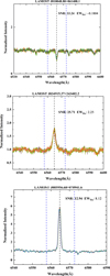 |
Fig. A.1 Examples of low-, moderate-, and high-activity stars showing the adopted ±25 A continuum windows and fixed 15 A integration region around the Hα line. The blue dashed vertical lines mark these spectral integration regions, illustrating the performance of our measurement method across different activity levels. |
All Tables
Stellar parameters of M dwarf stars obtained through calculation and cross-matching.
All Figures
|
Fig. 1 Hertzsprung – Russel diagram of M dwarfs. The left panel shows the relation between the effective temperature (Teff) and the surface gravity (log g). The metal-licity ([Fe/H]) is colored. The right panel shows the relation between the color index (GBP – GRP) and the apparent magnitude (MG). The number of stars is colored. |
| In the text | |
|
Fig. 2 Distribution statistics of the number of stars and spectra for each subclass. Left: bar chart showing the distribution of the number of stars in each subclass. Right: bar chart showing the distribution of the number of spectra for each subclass. |
| In the text | |
|
Fig. 3 Relation between Teff and EWHα. The stellar surface gravity is colored. Teff was obtained from cross-matching the TESS input catalog v8.2 using TOPCAT (Taylor 2020). The red line divides the stars into effective temperature intervals, indicating the median EWHα within each interval. |
| In the text | |
|
Fig. 4 Distribution of activity proportions for M dwarfs of different subtypes. The data labels represent the number of active stars. |
| In the text | |
|
Fig. 5 Left: bar chart showing the distribution of the stellar exposure counts. The x-axis label refers to the binned ranges of exposure counts per star. Right: bar chart displaying the statistics of the variability coefficients for stars. |
| In the text | |
|
Fig. 6 Equivalent width (EW) of the Hα line variation statistics. The left panel shows the distribution statistics of δEWHα ( |
| In the text | |
|
Fig. 7 Relation between EWHα, its standard deviation (σ EWHα), and the ratio of the standard deviation to EWHα is as follows (σEWHα/<EWHα>): The left panel illustrates the relation between EWHα and σEWHα, and the right panel shows the relation between EWHα and σEWHα/<EWHα>. The red line represents the median value within each interval. |
| In the text | |
|
Fig. 8 Hα variation in the selected examples. The left panel shows the spectrum that clearly displays the changes in the Hα line. The right panel visually presents the dynamic evolution of EWHα on short timescales, and the vertical red lines indicate the error bars. The colors of the spectral profiles in the left panel correspond to the points in the right panel, which are labeled with their respective heliocentric Julian dates, which allow a clear identification of the observation epochs. |
| In the text | |
|
Fig. 9 Distribution histogram of a double-Gaussian fit of the R′Hα value. The x-axis represents the R′Hα values of each star, and the y -axis represents the number of stars. |
| In the text | |
|
Fig. 10 Correlation between chromospheric activity indicators R′Hα and the Rossby number (Ro). The red and blue lines show the fit relation between these parameters. The color represents the stellar Teff. |
| In the text | |
|
Fig. 11 Two-dimensional and one-dimensional distribution of active stars based on the Hα line. The left panel illustrates the two-dimensional distribution of the ratio of active stars to the total number of stars in cylindrical galactocentric coordinates (R and Z), where the color indicates the active fraction. The right panel shows the relation between stellar activity proportions and the vertical distance from the Milky Way plane. The vertical red lines represent the error bars. |
| In the text | |
|
Fig. 12 Relation between stellar flare energy and duration. The left panel shows the relation between the flare energy and the duration for all flare data samples. The red line represents the fit result. The right panel shows the relation between Log(flare energy) and the duration for all samples. The color bar represents the number of flare events. |
| In the text | |
|
Fig. 13 Relation between flare energy and duration for M dwarf stars of different subtypes. |
| In the text | |
|
Fig. 14 Relation between the log flare energy and the flare duration for M dwarf stars of different spectral subtypes. |
| In the text | |
|
Fig. 15 Left panel: relation between the chromospheric activity indicator R′Hα and stellar starspots. Right panel: relation between EWHα and stellar starspots. |
| In the text | |
|
Fig. 16 Number distribution of the stellar flare duration and flare amplitude. The left panel shows the number distribution of stellar flare durations, and the right panel shows the number distribution of the flare amplitude. |
| In the text | |
|
Fig. 17 Percentage distribution of the flare event duration and amplitude in different ranges relative to the total sample. The left panel shows the distribution of the flare duration percentages, and the right panel shows the distribution of the flare amplitude percentages. |
| In the text | |
|
Fig. 18 Dynamic evolution of the EWHα on short timescales. The values of the EWHα energy and amplitude changes are shown, and the vertical red lines indicate the error bars. |
| In the text | |
|
Fig. 19 Examples of the Hα profile asymmetry in stellar redshift and blueshift integration regions for CME detection. Left: LAMOST J133213.26+505702.2. Right: LAMOST J030002.90+550653.0. The dashed red and green lines represent the integration boundaries, the dashed yellow and blue lines indicate the theoretical and actual peak positions of the Hα profile, and the light blue and red regions represent the integration areas. |
| In the text | |
|
Fig. 20 Spectral analysis of the stellar Hα lines and double-Gaussian fit. The left panel shows the preprocessed Hα spectra of the star, the middle panel presents the smoothed Hα spectra, and the right panel displays the contrast flux profile derived from the double-Gaussian fit. The lower panel illustrates the identified flare events in the stellar light curve along with a magnified view of the corresponding flare regions. |
| In the text | |
|
Fig. 21 Spectral analysis of the stellar Hα lines and double-Gaussian fit. The left panel shows the preprocessed Hα spectra of the star, the middle panel presents the smoothed Hα spectra, and the right panel displays the contrast flux profile derived from the double-Gaussian fit. |
| In the text | |
|
Fig. A.1 Examples of low-, moderate-, and high-activity stars showing the adopted ±25 A continuum windows and fixed 15 A integration region around the Hα line. The blue dashed vertical lines mark these spectral integration regions, illustrating the performance of our measurement method across different activity levels. |
| In the text | |
Current usage metrics show cumulative count of Article Views (full-text article views including HTML views, PDF and ePub downloads, according to the available data) and Abstracts Views on Vision4Press platform.
Data correspond to usage on the plateform after 2015. The current usage metrics is available 48-96 hours after online publication and is updated daily on week days.
Initial download of the metrics may take a while.