| Issue |
A&A
Volume 704, December 2025
|
|
|---|---|---|
| Article Number | A287 | |
| Number of page(s) | 13 | |
| Section | Extragalactic astronomy | |
| DOI | https://doi.org/10.1051/0004-6361/202555494 | |
| Published online | 16 December 2025 | |
ILLUSTRating red nugget assembly through observations and simulations
1
Instituto de Astrofísica de Canarias, Vía Láctea s/n, E-38205 La Laguna, Tenerife, Spain
2
Instituto de Física, Universidade Federal do Rio Grande do Sul, Av. Bento Gonçalves 9500, Porto Alegre R.S. 90040-060, Brazil
3
Departamento de Astrofísica, Universidad de La Laguna, E-38200 La Laguna, Spain
4
Centre for Astrophysics and Supercomputing, Swinburne University, John Street, Hawthorn, VIC 3122, Australia
★ Corresponding author: This email address is being protected from spambots. You need JavaScript enabled to view it.
Received:
12
May
2025
Accepted:
6
October
2025
Abstract
The properties of massive and compact early-type galaxies provide important constraints on early galaxy formation processes. Among these, massive relic galaxies, characterized by old stellar populations and minimal late-time accretion, are considered to be preserved compact galaxies from the high-z Universe. In this work, we investigate the properties of compact and massive galaxies (CMGs) using the TNG50 cosmological simulation, applying a uniform selection criterion that matches observational surveys at z = 0, z = 0.3, and z = 0.7. This approach provides a basis for direct comparisons with observed compact galaxies at each evaluated redshift. We classify CMGs according to their stellar mass assembly histories to investigate how compactness relates to dynamical properties and chemical enrichment across cosmic time. Our results show that simulated CMGs consistently follow the observed mass–size relation, with the number of compact galaxies increasing at higher redshifts; this number density follows the trend seen in observational data. In the dynamical context, while observations suggest that relic galaxies are outliers in the stellar mass–velocity dispersion plane, the simulated compacts show relatively uniform velocity dispersions across different accretion histories. Observed relics tend to be more metal-rich than other compact galaxies with extended star formation histories, deviating from the local mass–metallicity relation. In contrast, simulated compact galaxies are, overall, more metal-rich than the quiescent population, regardless of their accretion histories. We also find that the deviation of the simulated CMGs from the mass–metallicity relation decreases with increasing redshift. These findings suggest that the extreme characteristics of the CMGs in TNG50, particularly with regard to metal enrichment and dynamical properties, are less pronounced than those observed in real relic galaxies. However, the results offer a theoretical framework for assessing the properties of such extreme objects from different epochs, highlighting both alignment with and deviations between the models.
Key words: galaxies: evolution / galaxies: formation / galaxies: fundamental parameters
© The Authors 2025
 Open Access article, published by EDP Sciences, under the terms of the Creative Commons Attribution License (https://creativecommons.org/licenses/by/4.0), which permits unrestricted use, distribution, and reproduction in any medium, provided the original work is properly cited.
This article is published in open access under the Subscribe to Open model. This email address is being protected from spambots. You need JavaScript enabled to view it. to support open access publication.
1. Introduction
The two-phase scenario (e.g., Naab et al. 2009; Oser et al. 2010) for the formation and evolution of massive early-type galaxies (ETGs) has gained a new perspective with the advent of James Webb Space Telescope (JWST) data. The scenario involves an initial phase of formation occurring before z = 2, which is marked by the rapid growth of stellar mass through wet mergers, resulting in a phase with a high star formation rate (SFR), but without significant size growth (e.g., van Dokkum et al. 2015; Zolotov et al. 2015; Zibetti et al. 2020). Due to the rapid mass increase and the intense star formation episodes in this first stage of evolution, a massive and compact object is formed, known as a red nugget. Such objects are expected to quench rapidly and become passive. However, recent discoveries from JWST have revealed that quenching in massive galaxies was far more common during the first two billion years (z > 3), leading to higher-than-expected number densities of massive quiescent galaxies in the redshift range 3 < z < 5 (Carnall et al. 2024; Ito et al. 2024; Long et al. 2024). These high-z red nuggets will subsequently undergo a second phase during which they grow in size through the accretion of smaller satellites, creating the massive ETGs observed in the local Universe today.
Following this scenario, compact massive galaxies (CMGs) are thus expected to decrease in number density with decreasing redshift (e.g., Trujillo et al. 2009; Damjanov et al. 2015; Charbonnier et al. 2017), with the underlying expectation that CMGs in the local Universe are rare, as most will grow in size through mergers and accretion during the second phase. Nonetheless, local CMGs have been found in all environments (e.g., Trujillo et al. 2009; Poggianti et al. 2013; Grèbol-Tomàs et al. 2023). Their existence is explained by the stochastic nature of mergers; hence, it is expected that a small fraction of high-z red nuggets avoid significant accretion (Quilis & Trujillo 2013) during the second phase. In the extremely rare cases where the red nugget remains untouched over cosmic time, such CMGs are referred to as massive relic galaxies (Trujillo et al. 2009).
The search for these elusive ancient galaxies has revolved around small samples of local CMGs. Unfortunately, most of them proved to be younger systems (Trujillo et al. 2009; Ferré-Mateu et al. 2012; Poggianti et al. 2013). Some CMGs are promising, showing several characteristics similar to massive relics (e.g., Yıldırım et al. 2017; Grèbol-Tomàs et al. 2023; Clerici et al. 2024). However, only a few have been thoroughly investigated through detailed, multi-property analyses. Among them, PGC 032873, Mrk 1216, and NGC 1277 stand out as the most extensively studied cases of massive relic galaxies (Ferré-Mateu et al. 2017). Their disk-like symmetrical shapes show no signs of tidal streams, indicating no recent evident interaction signatures; all host extremely large supermassive black holes (Ferré-Mateu et al. 2015), present a bottom-heavy initial mass function (IMF), as suggested by Martín-Navarro et al. (2015), Ferré-Mateu et al. (2017), and have stellar populations and kinematics comparable with those of high-z red nuggets. The luminosity fraction of the hot inner stellar halo (or spheroid compactness) correlates strongly with merger history (Zhu et al. 2025, 2022), with merger-free galaxies displaying extremely compact spheroids, consistent with those seen in relic candidates (Moura et al. 2024; Zhu et al. 2025). In recent years, new promising relic candidates have emerged, supported by improved photometric selection techniques, deeper spectroscopic follow-up, and dedicated kinematics analysis (e.g., Grèbol-Tomàs et al. 2023; Zhu et al. 2025; Mills et al. 2025).
While massive relic galaxies are understood within the proposed theoretical scenario, it remains unclear how younger CMGs exist in the local Universe. To investigate this, Grèbol-Tomàs et al. (2023) searched for CMGs in MaNGA (DR17; Bundy et al. 2015) and classified them using machine learning approaches according to their star formation histories (SFHs), i.e., how rapidly and when they occurred. They report that CMGs can be classified into three groups, one of which closely resembles massive relics. The other types show distinctly different SFHs, metallicities, and α-abundances. Some exhibit extended SFHs similar to lower-mass ETGs, while others present rapid, though delayed, formation in time (late bloomers). More recently, Mills et al. (2025) searched for CMGs in the Sloan Digital Sky Survey (SDSS), demonstrating that these objects exist in larger numbers than previously observed. With upcoming all-sky surveys such as Euclid, we expect that the number of CMGs and known relics will change.
As expected from the two-phase scenario, there is a significant increase in the number density of CMGs between z = 0 and z ∼ 2, as galaxies have had less time for the accretion phase (Damjanov et al. 2009; Charbonnier et al. 2017; Tortora et al. 2018; Lisiecki et al. 2023). This means that massive relic galaxies should also exist at intermediate redshifts. The INSPIRE project (Spiniello et al. 2021) has focused on investigating CMGs at intermediate redshifts to create the first catalog of spectroscopically confirmed massive relic galaxies between 0.1 < z < 0.5. To date, this project has provided a detailed characterization of the kinematics, stellar populations, low-mass end of the IMF, and environment (D’Ago et al. 2023; Spiniello et al. 2024; Martín-Navarro et al. 2023; Maksymowicz-Maciata et al. 2024; Scognamiglio et al. 2024) of CMGs in that redshift range. One key finding from this project is that massive relic galaxies tend to be more metal-rich compared to non-relics and also exhibit higher velocity dispersions (D’Ago et al. 2023), trends also seen in the local CMGs of Grèbol-Tomàs et al. (2023).
Following the idea that a “degree of relicness” (DoR) exists in local massive relics (Ferré-Mateu et al. 2017), and given the three clearly distinctive types of CMGs identified by Grèbol-Tomàs et al. (2023), the CMGs from the INSPIRE project were classified according to a parametrization of the DoR (Spiniello et al. 2024). The DoR is defined as a dimensionless value ranging from 1 to 0, where 1 represents the most extreme case of a relic galaxy (e.g., NGC 1277 in the local Universe is the prime example of an extreme relic, with a DoR of almost 1), while 0 represents a galaxy still forming stars. They found that the DoR correlates with stellar velocity dispersion, metallicity, [Mg/Fe] ratio, and age. In addition, Scognamiglio et al. (2024) observe that CMGs reside both in clusters and in the field, similar to findings in the local Universe (e.g., Poggianti et al. 2013; Peralta de Arriba et al. 2016; Cebrián & Trujillo 2014; Moura et al. 2024). However, there is a slight preference for galaxies with a very low DoR (< 0.3) to reside in under-dense environments, while the most extreme relics tend to reside in the central regions of clusters.
At even higher redshifts, the VIMOS Public Extragalactic Redshift Survey (VIPERS, Scodeggio et al. 2018), identified 77 CMGs in the redshift range 0.5 < z < 1.0. This catalog provides spectroscopically confirmed galaxies that follow the mass–size and quiescence criteria for red nuggets at these intermediate redshifts (Siudek et al. 2023; Lisiecki et al. 2023). Lisiecki et al. (2023) emphasize the impact of source compactness limits on selection, with sample size varying by up to two orders of magnitude depending on the criterion used. It is also expected that the fraction of red nuggets in clusters increases over time, as red massive normal-sized galaxies lose their envelopes through stripping (Siudek et al. 2023; Zhu et al. 2025). The resulting number density found in VIPERS exceeds estimates for the local Universe but remains below values at z > 2, bridging the gap at intermediate redshifts.
The properties of CMGs, particularly the massive relic variety, are also discussed in several numerical simulations (Wellons et al. 2015; Stringer et al. 2015; Peralta de Arriba et al. 2016; Flores-Freitas et al. 2022; Moura et al. 2024; Zhu et al. 2025). Using the Illustris TNG50 simulation (e.g. Pillepich et al. 2019; Nelson et al. 2019), Flores-Freitas et al. (2022) identified five candidates for massive relic galaxy that match the observed relics in metallicity and morphology. Using TNG50 simulations, Moura et al. (2024) analyzed a sample of CMGs, identifying relics as those with less than 10% satellite accretion throughout their evolution. Their analysis of internal dynamics and environment reveals that merger signatures can be detected through the kinematics of the inner stellar halo, providing a new signature for identifying extreme relics. Zhu et al. (2025) show that in TNG50, the hot inner stellar halo fraction correlates strongly with merger history. A very low halo fraction combined with a dynamically cold disk signals a merger-free relic. Their study identifies seven compact galaxies from Yıldırım et al. (2017) consistent with this scenario.
Cosmological simulations offer the advantage of investigating the red nugget progenitors of the local CMGs and tracing back their evolutionary pathways. In this work, we used the TNG50 simulation to select CMGs in four redshift bins using similar primary selection criteria applied to observations. This approach allows for a consistent comparison of stellar populations and kinematics between simulated and observed CMGs at different epochs, including z = 0 for local relations, z = 0.3 (for comparison with INSPIRE), and z = 0.7 (for comparison with VIPERS). Although no red nugget catalog is available for z ∼ 2, we include this redshift bin because it has traditionally been adopted as the reference point for the onset of the second-phase evolutionary scenario. However, recent JWST results suggest that compact massive galaxies could already be present at earlier epochs (z ∼ 3–4; Carnall et al. 2023; Nanayakkara et al. 2025), indicating not necessarily an earlier onset of their formation, but that some systems may have formed more rapidly than previously thought. For consistency with the established two-phase framework, we therefore use z = 2 as our starting point.
Our goal is to draw a parallel between observed and simulated CMGs by examining their mass–size, mass–velocity dispersion, and mass–metallicity relations, highlighting aspects such as compactness, dynamics, and chemical abundances across different cosmic epochs and their relation with different assembly histories. This paper is organized as follows. We introduce the simulation sample selection and observational data in Section 2, analysis and discussion are presented in Section 3, and we present a summary and conclusions in Section 4. Throughout the paper, we assume the cosmological parameters of Planck Collaboration XIII (2016) for a Lambda cold dark matter (ΛCDM) cosmological model with H0 = 67.74 km s−1 Mpc−1, Ωm = 0.30, and ΩΛ = 0.69.
2. Sample selection and main properties
We explored the formation and evolution of CMGs by analyzing the SFHs from simulations and observations at four redshifts: z = 0, z = 0.3, z = 0.7, and z = 2. We aimed to assess how structural properties, such as stellar mass, size, metallicity, and velocity dispersion, relate to the accretion histories, providing insight into their evolutionary pathways. Here, we describe the parameters used to select the sample and the main properties analyzed.
2.1. Observations
Traditionally, CMGs have been sought by applying mass and size criteria. Although not all studies have followed the exact same criteria (see Charbonnier et al. 2017 and Lisiecki et al. 2023 for a discussion), the initial, most restrictive criteria from Trujillo et al. (2009) defined CMGs as having M★ ≥ 8 × 10¹⁰ M⊙ and Re ≤ 1.5 kpc. Later studies, such as INSPIRE, have allowed for a slightly larger size constraint, limiting it to 2 kpc. Some later studies also incorporated a third criterion, based on the surface density relation established by Barro et al. (2013). This compactness parameter is defined as Σ1.5 = M [M⊙]/(Re [kpc])1.5, where the stellar mass contained within the effective radius is considered. We used Σ1.5 > 10.3 dex for the selection (Barro et al. 2013; Grèbol-Tomàs et al. 2023; Mills et al. 2025). This relation provides a compactness parameter that is consistent across all adopted redshifts.
For the local Universe sample, we considered the three confirmed massive relic galaxies: NGC 1277, PGC 032873, and Mrk 1216 (Ferré-Mateu et al. 2017; Trujillo et al. 2014). All structural properties, such as stellar masses, stellar population parameters, and kinematics, were taken from Ferré-Mateu et al. (2017). We also included the 37 MaNGA CMGs from Grèbol-Tomàs et al. (2023), obtained by selecting galaxies with a surface mass density threshold Σ1.5 > 10.3 dex and Re < 2 kpc. Using stacked spectra within 1 Re, they measured recessional velocities and stellar velocity dispersions and derived stellar population properties, including age and total metallicity. Through the analysis of the stellar population and kinematic properties, they classified the galaxies into three groups based on their assembly history: Group A, comprising very old galaxies (> 12 Gyr) with early and steep SFHs (similar to massive relics); Group B, containing intermediate-age galaxies and more extended SFHs (≈8 Gyr); and Group C, young galaxies (≈5 Gyr), referred to as “late-bloomers”, as they formed rapidly but relatively late in cosmic time.
At local-to-intermediate redshift, we used the entire sample from the INSPIRE project (Spiniello et al. 2021), consisting of 52 CMGs at redshifts between 0.1 and 0.5, all with effective radii smaller than 2 kpc and stellar masses greater than 6 × 10¹⁰ M⊙. This sample includes optical and near-infrared photometry from the KiDS and VIKING surveys (Edge et al. 2013), structural parameters (Roy et al. 2018), and stellar masses inferred through spectral energy distribution (SED) fitting using the u, g, r, and i bands (Tortora et al. 2018; Scognamiglio et al. 2020). The INSPIRE galaxies have estimates of integrated stellar velocity dispersions within 1 Re, [Mg/Fe] measurements obtained from line indices, as well as mass-weighted stellar ages and metallicities derived from full spectral fitting. This sample, similar to the MaNGA sample, shows a variety of SFHs, parametrized by a varying DoR (Spiniello et al. 2024).
Finally, we used data from VIPERS (Scodeggio et al. 2018) for the intermediate redshift regime. For this study, we used a subset of 77 CMGs from the VIPERS catalog at 0.5 < z < 1.0 (Lisiecki et al. 2023), constructed by selecting objects that are both massive and compact (M★ > 8 × 10¹⁰ M⊙, Re < 1.5 kpc), and by including passiveness criteria based on both spectroscopic and photometric analyses (see Lisiecki et al. 2023 and Siudek et al. 2023).
All observational data described here are shown in Fig. 1, represented by diamond-shaped markers, separated by redshift bins. The figure also presents the stellar mass–size relation of observed galaxies from van der Wel et al. (2014) at each redshift of interest.
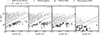 |
Fig. 1. Stellar mass–size relation across redshift bins. All TNG50 subhalos are shown as light gray circles in the background, while selected compact subhalos are represented by dark gray circles. Observational CMGs from the different samples are indicated with white diamond markers. The solid black lines follow the mass–size relation from van der Wel et al. (2014), while the dashed gray lines highlight the selection region for the simulated sample (Re < 2 kpc, log Σ1.5 > 10.3 dex). |
2.2. Simulations
We used the IllustrisTNG suite of cosmological magnetohydrodynamical simulations (Marinacci et al. 2018; Naiman et al. 2018; Nelson et al. 2018; Pillepich et al. 2018; Springel et al. 2018) to select our sample of simulated CMGs. These simulations were performed using the moving-mesh code AREPO (Springel 2010), with a comprehensive overview provided in the release paper by Nelson et al. (2019). In this work, we focus on TNG50, (e.g., Pillepich et al. 2019; Nelson et al. 2019), the smallest cosmological volume in the suite (Lbox = 51.7 cMpc), which offers the highest resolution (Pillepich et al. 2018). Although the smaller volume limited the number of candidates, the higher resolution allowed us to study the structural and dynamical properties compared to observations.
Stellar masses are computed as the total mass of bound star particles within a given aperture, while galaxy sizes are typically defined based on the 3D half-mass radius of the stellar distribution. In this context, the radius corresponds to the half-mass radius, which encloses half of the total stellar mass of the galaxy. Adopting the 3D half-mass radius provides a consistent and physically motivated definition of size within the simulation, ensuring that the selected sample is genuinely compact, regardless of the observational size definition. Further discussion of mass–size comparisons between simulations and observations can be found in Genel et al. (2018). To select our simulated sample, we selected all subhalos with stellar masses above 1010 M⊙ and sizes Re < 2kpc to compare with the observational sample described above. We applied the surface density criterion from Barro et al. (2013) to select all compact subhalos from this initial selection. The final selection of subhalos is shown in the mass–size plane in Fig. 1, compared to the observational data. This selection was applied independently at each redshift (z = 0, 0.3, 0.7, and 2), without following the merger trees of the subhalos. Thus, while some galaxies selected as compact at higher redshift may correspond to progenitors of z = 0 galaxies, this correspondence was not systematically tracked or required by our selection. Our focus was to obtain the population of CMGs at each cosmic epoch based solely on their properties at each snapshot, independent of whether their descendants or progenitors remain compact.
We obtained the same mass range for MaNGA galaxies and subhalos at z = 0, with the most massive galaxies at this redshift being the three spectroscopically confirmed relics. At z = 0.3 and z = 0.7, the stellar mass range for observed compacts is generally concentrated at the high-mass end (M★ ≈ 1011 M⊙), while the simulated compacts have, on average, lower stellar masses than the observed ones. The simulated galaxies may not reach this high-mass end because of the limited volume of the simulation. We observe an increase in the number of subhalos and compact galaxies with increasing redshift. This is due to the mass–size evolution, in which galaxies at earlier times tend to be more compact than those observed today.
In addition to the mass–size and compactness selection criteria, we also analyzed the morphology of the simulated galaxies through visual inspection to ensure that none showed clear merger signatures. Following this inspection, we obtained a final sample of nine compact massive subhalos at z = 0, 13 at z = 0.3, 25 at z = 0.7, and 36 subhalos that match the mass–size relation and the concentration parameter at z = 2 (representing the red nugget stage, i.e., the onset of the second phase). Fig. 2 shows examples of subhalos at each redshift bin from the simulated sample, together with real compact galaxies at the same redshifts.
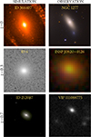 |
Fig. 2. Example of the selected sample of compact TNG50 simulated (left column) and observed (right column) galaxies across redshift bins: z = 0 (top row), z = 0.3 (middle row), and z = 0.7 (bottom row). Observed galaxies include NGC 1277 (top-right, HST ACS/WFC instrument), Spiniello et al. 2024 (middle-right), and VIPERS (bottom-right). |
Our simulated sample shows an increase in the number of selected CMGs with increasing redshift. By calculating their number density across redshift bins in Fig. 3, we demonstrate agreement with the established trend of increasing compact galaxy abundance at comparable redshifts, as reported by van der Wel et al. (2014) and Barro et al. (2013). We limited our selection to z ≤ 2, as our analysis focuses on this redshift interval. This approach also offers a direct comparison with observational estimates from other works on compact galaxies (e.g., Lisiecki et al. 2023; Scognamiglio et al. 2020; van der Wel et al. 2014; Barro et al. 2013; Ferré-Mateu et al. 2017). It is important to emphasize that the compact selection criteria vary across different studies (for a discussion, see Charbonnier et al. 2017; Lisiecki et al. 2023). In addition, since the number density depends on the survey volume, the limited size of the TNG50 simulation also affects the results. Therefore, direct expectations regarding the agreement between the simulated and observed number densities at each redshift should be interpreted with caution.
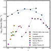 |
Fig. 3. Number density of CMGs as a function of redshift, in units of co-moving Mpc−3. The black line and markers represent the TNG50 CMGs from this work. Colored lines and markers correspond to observational estimates from VIPERS (Lisiecki et al. 2023) in red, Scognamiglio et al. (2020) in orange, Damjanov et al. (2014) in green, van der Wel et al. (2014) in purple, Barro et al. (2013) in blue, and Ferré-Mateu et al. (2017) in dark green for the local relics, and magenta for Grèbol-Tomàs et al. (2023) compacts. Simulated CMGs show an increasing number density with redshift, consistent with models predicting more compact objects in the early Universe. A similar trend is seen in the observational data. |
The stellar velocity dispersion values (σ★) of simulated galaxies in the TNG simulations are calculated from the particle distribution within each subhalo. The SUBFIND algorithm (Springel 2010; Dolag et al. 2009) uses the spatial x, y, and z center positions, together with the central velocities, to compute the mass-weighted 3D velocity dispersion for each particle type (i.e., dark matter, gas, and stellar particles). Sohn et al. (2024b) investigated the stellar velocity dispersion of quiescent massive subhalos in IllustrisTNG, focusing on potential systematic effects. They analyzed the dependence of velocity dispersion on simulation resolution, viewing axes, and the identification of member stellar particles. Their findings do not reveal significant discrepancies in σ★ across these variations. They further showed that the scatter in the velocity-dispersion distribution is generally larger than the systematic uncertainties. Interestingly, in the M★ − σ★ relation, the observed values from SDSS DR12 (Alam et al. 2015) data at z < 0.2 are typically 40%–50% higher than the simulated σ★ values for a given stellar mass. Fig. A.1 shows a histogram of the distribution of stellar mass, effective radius, and stellar velocity dispersion for both simulated and observed samples, and Table A.1, listing all relevant information on the simulated sample, is also shown in the appendix.
The TNG (and Illustris) simulations model astrophysical processes such as radiative cooling and heating of the interstellar medium (ISM), stellar feedback, black hole growth, and active galactic nuclei (AGN) feedback, which include models of stellar evolution and chemical enrichment. In such models, star formation and pressurization of the multiphase ISM follow Springel & Hernquist (2003), where gas exceeding a density threshold (n > 0.13 cm3) forms stars according to an IMF from Chabrier (2003). The dense star-forming ISM was treated using a two-phase effective equation-of-state model (Pillepich et al. 2018). Newly formed stars inherit the metallicity of the gas from which they form. As they evolve, they return both mass and metals to the ISM through supernovae and asymptotic giant branch stars, following tabulated mass and metal yields. The model employs cell-centered magnetic fields to solve the equations of ideal magnetohydrodynamics (Pakmor et al. 2011) and tracks the evolution of nine chemical elements (H, He, C, N, O, Ne, Mg, Si, and Fe). Details on the implementation and metal tagging can be found in Pillepich et al. (2018) and Naiman et al. (2018). The metallicity of each stellar particle in TNG was calculated as the ratio of the mass of heavy elements to its total mass at the time of formation, reflecting the chemical composition of the gas cell from which it originated. This intrinsic metallicity is stored as part of the stellar particle’s properties and represents the local enrichment at the formation site.
Garcia et al. (2024) investigated the intrinsic differences in the derivation of metallicity in simulations and observations. They also analyzed the gas-phase and stellar metallicities in the Illustris, IllustrisTNG, and EAGLE (Schaye et al. 2015; Crain et al. 2015) cosmological simulations to study their dependence on star formation and stellar mass. Although these simulations share common approaches to modeling the ISM, star formation, and metal enrichment, they differ in the feedback processes that shape both the stellar mass–gas-phase metallicity relation and the stellar–mass metallicity relation (MZ★R). Garcia et al. (2024) compared the simulations with observational data from Gallazzi et al. (2005) and Panter et al. (2008), emphasizing that such comparisons are not straightforward. Specifically, calculating metallicities by averaging the metal content of star particles weighted by their mass, as performed in all three analyzed simulations, yields higher stellar metallicities than those obtained using radiative transfer codes, which better approximate mock galaxy observation (Guidi et al. 2016). Their findings indicate that MZ★R at z = 0 and at higher redshifts is systematically higher than in observational data. Nelson et al. (2018) notes that a robust comparison of TNG stellar metallicities with SDSS fiber-derived spectral values requires more advanced forward modeling. The study also points out that the simulated stellar metallicities do not align with observations, partly because of a shortage of present-day, low-mass dwarf systems formed within the past billion years, which likely contributes to the observed discrepancy. However, the authors emphasize that this discrepancy probably results from an overly simplistic comparison. An alternative analysis using consistent fits to mock SDSS fiber spectra is necessary to enable a fair comparison between observations and simulations.
We note that we did not aim to directly compare observations and simulations of CMGs quantitatively, as the methods used to derive their parameters differ. Additionally, no equivalence exists in terms of environment, universe volume, sample size, or resolution between the observational and simulation data.
The most appropriate way to interpret this analysis – and any comparative analysis between observation and simulation – is to qualitatively assess whether the trends generally converge or diverge, taking into account the limitations and methodological differences in studying the same property. By grouping the samples according to their star formation histories, we evaluated the behavior of the simulated populations at each redshift and tested whether they follow similar observed trends. Consequently, we did not attempt to identify simulated analogs of observed CMGs or perform one-to-one comparisons but instead characterized the populations in each dataset and compared their general behavior. This perspective informs the subsequent discussion of the results.
3. Analysis
3.1. Timescale of evolution
The two-phase scenario allows for different evolutionary pathways in which mergers can prolong the SFH to varying degrees. Galaxies that assembled most of their mass early in cosmic history tend to exhibit more extreme properties, including higher velocity dispersions, larger black hole masses, and over-solar metallicities, and are generally more extreme than galaxies with extended SFHs. Given the diversity of formation timescales among massive galaxies, a range exists in the degree to which a CMG can be considered a relic. This metric, known as the degree of relicness (DoR; Ferré-Mateu et al. 2017), has been explored and parametrized for both the MaNGA and INSPIRE samples.
Grèbol-Tomàs et al. (2023) used machine learning tools to classify the SFHs of the MaNGA CMG sample into distinct types, accounting for both their SFHs and structural parameters. Applying a K-means algorithm, they identified three distinct groups. Group A comprised very old, compact, metal-rich galaxies, all showing rapid SFHs with very early assembly, consistent with their high α-enhancement values. The other two groups (B and C) showed different levels of extended SFHs: one was more similar to low-mass ETGs (i.e., showing steady extended SFHs), while the other displayed a rapid but extremely delayed SFH (similar to the younger “late bloomer” CMGs identified by Ferré-Mateu et al. (2012)). Galaxies in groups B and C generally had lower metallicities, less enhanced α-abundances, and lower velocity dispersions.
In the INSPIRE survey, galaxies from the first data release (DR1; (Spiniello et al. 2021)) were classified into three categories based solely on their SFHs: “extreme relics”, which fully assembled their stellar mass by z = 2; “relics”, which assembled at least 75% of their stellar mass by z = 2; and “non-relics”, which had less than 75% of their mass assembled by z = 2. This quantification of the DoR was later refined in the final DR5 by incorporating both the average SFH and the cosmic time at which most of the stellar mass was assembled (see Spiniello et al. 2024). A higher DoR (i.e., > 0.7) indicates an earlier formation epoch, with minimal contribution from accreted stars or those formed during later star-forming episodes. A lower DoR indicates that, although a portion of the stars are old and formed at early times, a significant fraction formed later, with varying ages and metallicities, reflecting extended SFHs. For the exemplary case of NGC 1277, the DoR is estimated to be 0.95 (Spiniello et al. 2024). Nonetheless, the choice of parametrization does not significantly affect the correlations with other stellar parameters, such as metallicity, IMF, and stellar velocity dispersion.
Taking into account the different definitions of DoR, we adopt a simplified version with three distinct categories. The relic class comprises galaxies that exhibit early and fast formation timescales and is hereafter represented in red. This category corresponds to galaxies in Group A of the MaNGA sample and those with DoR ≥ 0.5 in INSPIRE. Within this relic class, the extreme cases are those that present the earliest and most rapid formation timescales. This extreme class is represented by dark red in the following figures and corresponds to the extreme cases of Group A for MaNGA (see Fig. 4) and to galaxies with DoR ≥ 0.7 in the INSPIRE data. Lastly, the non-relic class comprises CMGs with a low likelihood of being relics given their late and/or more extended SFHs (DoR < 0.5 and Groups B and C in MaNGA), and is depicted in blue throughout the remaining figures.
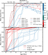 |
Fig. 4. Stellar mass assembly for the simulated and observed samples at z = 0. The upper panel shows the stellar mass fraction over time for each compact subhalo selected from TNG50, color-coded by the stellar mass growth fraction since z = 2. The lower panel shows the stellar mass assembly over time for the MaNGA compact galaxies of Grèbol-Tomàs et al. (2023), color-coded by group: blue represents Groups B and C, which show extended and/or late SFHs; red represents galaxies in their Group A, which exhibit early and rapid formation (and thus negligible accretion after z = 2); dark red indicates extreme cases, where the galaxy is fully assembled early on (with < 10% accreted material). In both panels, the dashed vertical black line indicates z = 2 and the dashed horizontal gray line indicates the stellar mass fraction of 90%. |
We adopted a similar approach for the simulations, reconstructing the evolution of stellar mass over time through the SUBLINK merger tree, which traces the progenitors of the local subhalos (Rodriguez-Gomez et al. 2015). This method provides the stellar mass assembly over time for each subhalo, as shown in the upper panel of Fig. 4. Although it is in principle possible to recover a DoR from these SFHs, as in the observations, this procedure is not straightforward. Although simulated galaxies display clearly distinct SFHs, their final assembly times and the fraction of mass assembled within 3 Gyr (used in INSPIRE to parametrize the DoR) are less steep than in observations, leading to lower DoR values for all simulated CMGs. This difference is illustrated in Fig. 4, which compares the assembly histories of simulated and observed CMGs.
The simulations do not produce subhalos as early as seen in observations, requiring longer times to complete their build-up and exhibiting very low levels of star formation until recent epochs. Conversely, observations may be biased toward faster build-up, as the derivation of SFHs strongly depends on the adopted simple stellar population (SSP) models. This difference may partly explain the discrepancy with the simulations. Another factor to consider is the stripping process. Environmental effects and tidal forces can affect the estimated mass over time. Consequently, the mass obtained in simulations over time is not determined in the same way as in observations, where direct accounting for stripping is not possible. Ultimately, some CMGs result from stripping processes (Zhu et al. 2025) rather than solely from a lack of mergers during early epochs. We highlight these cases in Appendix A, where we calculate the SFHs for all simulated samples together with their size and mass growth (see Figure A.2).
To ensure a fair comparison, we focused on the assembly history during the second phase, since z = 2, for the simulated sample, as described above. For this purpose, we calculated the stellar mass growth fraction, fmass growth, defined as (M★, z − M★, z = 2)/M★, z = 2. This quantifies the stellar mass acquired during the second evolutionary phase of massive galaxies (from z = 2 to the redshift of interest in each bin). The upper panel of Fig. 4 shows the mass assembly over cosmic time for the nine selected compact subhalos at z = 0, color-coded by this fmass growth.
We used fmass growth to classify our subhalos into the three classes. For the relics class, we included CMGs with less than 20% mass growth or accretion, while we considered fmassgrowth ≤10% for the extreme relics class. The non-relic class comprised simulated CMGs with higher mass growth and, consequently, higher accretion fractions (e.g., ≥20%). The 10% threshold for the extreme cases was chosen following Moura et al. (2024), who used it to differentiate relics from other CMGs in TNG50 based on their kinematics. Using three semi-analytical models, Quilis & Trujillo (2013) also quantified the fraction and number density of massive galaxies formed at z > 2 with less than 10% and 30% stellar mass growth. They found that fewer than 2% of galaxies formed by z ≈ 2 have remained nearly unchanged, accreting no more than 10% of their mass. This extreme threshold is appropriate for simulations and is also consistent with the estimated maximum ex situ accretion of NGC 1277 (Beasley et al. 2018), the most extreme relic galaxy known in the local Universe. These threshold values are also directly compatible with the original INSPIRE definition, although in that case the limit was 25%.
3.2. Stellar mass – stellar velocity dispersion relations
One of the main results from INSPIRE is that the DoR strongly correlates with the integrated stellar velocity dispersion. Relic galaxies exhibit higher velocity dispersions compared to non-relics and normal-sized ETGs of similar stellar mass (Scognamiglio et al. 2024; Maksymowicz-Maciata et al. 2024; Mills et al. 2025), and thus σ★ can be used to select relic galaxies. This trend is also observed in Grèbol-Tomàs et al. (2023), where Group A galaxies (classified here as relics) display the highest velocity dispersions compared to other groups, standing out as clear outliers from the local scaling relation. This is shown in Fig. 5, which presents the σ★ and stellar mass relation for both simulated and observed galaxies at each z-bin. Here, we assume that there is no significant evolution with cosmic time for this relation, as Cenarro & Trujillo (2009) showed that spheroidal galaxies with M★ > 1011 M⊙ at z ≈ 1.6 exhibit σ★ values similar to those of present-day galaxies. The MaNGA and INSPIRE CMGs are color-coded according to their respective groups (see Sect. 3.1), while simulated CMGs are color-coded by their stellar mass growth since z = 2, as indicated by the color bar. The simulated CMGs in the z = 2 bin are left uncolored, as they represent the starting point of the second phase from which the mass growth fraction is computed to assign the classes in the simulations.
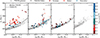 |
Fig. 5. Stellar mass–stellar velocity dispersion relations for simulated and observed galaxies in the different redshift bins. The dashed black line represents the median σ★ for all TNG50 quiescent subhalos, while the solid black line corresponds to the Zahid et al. (2016) relation across all redshifts. All TNG50 subhalos are shown as gray dots, with the compact sample color-coded by their mass growth since z = 2 (except for the final bin, which is considered he starting point and is therefore left uncolored). Observational data are represented by diamonds, color-coded as follows: dark red for the extreme relics (e.g., extreme cases of group A for MaNGA, DoR > 0.7 for INSPIRE); red for relics (remaining group A of MaNGA and INSPIRE galaxies with 0.5 < DoR < 0.7); and blue for the non-relic group (classes B and C of MaNGA, DoR < 0.5 for INSPIRE). |
Before drawing any conclusions, we note the caveats associated with the intrinsic differences between observations and simulations. Sohn et al. (2024a) finds discrepancies in the M★ − σ★ relation, with observed galaxies exhibiting velocity dispersions 40–60% higher than those in simulations. They attribute this to simulated clusters (from TNG300) containing roughly 60% fewer subhalos than observed clusters at the same stellar mass limit. Combined with intrinsic differences in the methods to measure this parameter, this results in a simulated velocity dispersion distribution that falls below the observed one, with a much smaller scatter, as shown in Fig. 5. Despite this caveat, our aim was to compare the behavior of the different classes, regardless of their exact σ★ values.
As expected, the MaNGA and INSPIRE galaxies show a dispersion in the σ★ at a given stellar mass. The extreme classes exhibit much higher σ★ than the rest, while the non-relics mostly follow the expected relation. No measurements for σ★ are available for the VIPERS sample; therefore, they are not included in this figure. We do not observe a clear trend among the simulated CMGs linking the extreme class to outlier behavior relative to the non-relic class. Although the highest σ★ values at z = 0.7 are associated with extreme cases, considerable scatter remains. Overall, we find that our CMGs for all classes generally exhibit similar and comparable σ★ values. In the future, the red nugget data from JWST will facilitate more accurate observational comparisons at z = 2. Naturally, a larger simulated sample is required for a more robust analysis across all redshifts.
In addition, environmental effects, such as dark matter halo mass and variations in velocity dispersion functions between field and clusters, influence velocity dispersion (Zahid et al. 2018; Sohn et al. 2024b). Intrinsic factors, such as black hole mass, also play a role (Gebhardt et al. 2000; Ferré-Mateu et al. 2015). Therefore, differences in velocity dispersion functions reflect both intrinsic and environmental impacts on galaxy evolution. Another important consideration is that velocity dispersion is calculated differently in simulations and observations. In simulations, the computed value does not refer solely to the central region of galaxies, which represents a source of incompatibility between the methods.
3.3. Stellar mass – stellar metallicity relations
Massive relic galaxies consistently exhibit high central metallicities and enhanced [Mg/Fe] abundance ratios, indicative of rapid and early SFHs (Ferré-Mateu et al. 2017; Grèbol-Tomàs et al. 2023; Maksymowicz-Maciata et al. 2024; Spiniello et al. 2024; Mills et al. 2025). Compared to non-relic CMGs, relics stand out for their uniformly elevated chemical signatures and shallower metallicity gradients (Ferré-Mateu et al. 2017; Mills et al. 2025). These properties are frequently accompanied by evidence of a bottom-heavy IMF, inferred from absorption features sensitive to low-mass stars (Martín-Navarro et al. 2015; Ferré-Mateu et al. 2017; Martín-Navarro et al. 2023). Further analysis reveals a correlation between the DoR, which quantifies the fraction of stellar mass formed at z > 2, and the IMF slope. Compact systems with higher DoR values exhibit more bottom-heavy IMFs, suggesting that the conditions prevailing during early cosmic times significantly influence the IMF (Martín-Navarro et al. 2023; Maksymowicz-Maciata et al. 2024; Mills et al. 2025).
Fig. 6 presents the stellar metallicity [M/H] as a function of stellar mass, together with reference mass–metallicity relations at different redshifts. The adopted relations from Gallazzi et al. (2005) and Gallazzi et al. (2014) are shown for the corresponding z-bins, with their intrinsic scatter represented by shaded regions. Simulated and observed CMGs are color-coded following the scheme in Fig. 5, distinguishing extreme, relic, and non-relic systems. A shift of −0.2 dex was applied to the stellar metallicities of galaxies with M★ > 1010 M⊙, following Nelson et al. (2019). Their mock analysis of SDSS-like spectra revealed a systematic underestimation of ∼0.2 dex in this mass range. Applying this correction provides a more consistent alignment of metallicity estimates across datasets, although it precludes a more quantitative comparison of these values.
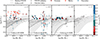 |
Fig. 6. Stellar mass – total stellar metallicity for simulated and observed galaxies. Symbols and colors are as in Fig. 5. A shift of −0.2 dex was applied to the stellar metallicities of simulated subhalos following Nelson et al. (2019). The dashed black line indicates the median stellar metallicity of quiescent subhalos in TNG50. Shaded regions correspond to the local stellar metallicity relations from Gallazzi et al. (2005); the solid black line follows Gallazzi et al. (2005) for z = 0 and z = 0.3, and Gallazzi et al. (2014) for z = 0.7. Observed relics are more metal-rich than other compact galaxies, deviating from the local mass–metallicity relation, while simulated compact galaxies are consistently more metal-rich than the quiescent population, independent of their SFHs. |
In terms of the general trend in Fig. 6, we observe that at z = 0, CMGs classified as extreme and relic in the MaNGA sample all lie above the average metallicity trend of Gallazzi et al. (2005). A similar behavior is seen in the simulated extreme and relic galaxies, which are predominantly located above the mean metallicity line for quiescent galaxies in TNG50. In comparison, the selected CMGs occupy a more metal-rich region relative to the general trend of the remaining galaxy population, regardless of their SFHs. This behavior appears to hold across all redshifts analyzed for the simulated CMGs. For galaxies that are neither relics nor extreme, this clear deviation from the scaling relations may indicate that they are galaxies that have undergone external processes such as stripping, which can remove part of their stellar mass while preserving the higher central metallicities of the original galaxy (e.g., Ferré-Mateu et al. 2021; Grèbol-Tomàs et al. 2023). Indeed, our sample of simulated CMGs shows evidence of stellar stripping at varying levels, as illustrated by the changes in the mass fraction over time in the upper panel of Fig. 4. By tracking stellar assembly in the simulations, we identify cases where a decrease in stellar mass is accompanied by a reduction in effective radius; these correlations are detailed in Appendix A.2. Since our compact galaxy selection is based solely on the mass–size relation at a given redshift, an ETG with a normal size (non-compact) at early times could undergo strong stripping and ultimately be classified as a suitable CMG in our selection. The correlations between galaxy stripping and satellite accretion fractions were investigated by Moura et al. (2024), who show that galaxies in high-density environments naturally accrete more satellites and tend to undergo more stripping.
To investigate the most metal-enhanced systems at each redshift, we next analyzed the deviation in stellar metallicity (Δ dex) of individual galaxies relative to the median mass–metallicity relation at each z-bin in Fig. 6. For each galaxy, the Δ dex values were calculated by subtracting the interpolated median metallicity at its corresponding stellar mass. Fig. 7 shows the resulting distribution, where we identify extreme outliers as galaxies with Δ dex values above the 90th percentile within their respective redshift bins. Although, by definition, approximately 10% of the galaxies should fall into this category, the actual fractions ranged from 11% to 15%, depending on the redshift. At low redshift (z = 0), the threshold for extreme deviation was Δ dex > 0.203, with a mean Δ dex of 0.245 among the extreme objects, indicating a small but highly enriched population. With increasing redshift, the 90th percentile Δ dex threshold decreases (e.g., Δ dex > 0.092 at z = 2) and the average deviation among the extreme galaxies becomes more modest (∼0.11 dex). This trend suggests that at earlier cosmic times even the most metal-rich galaxies deviate less significantly from the population median, possibly reflecting a narrower range of chemical enrichment or more homogeneous evolutionary pathways at high redshift.
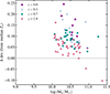 |
Fig. 7. Deviation of stellar metallicity from the simulated quiescent median relation as a function of stellar mass for compact galaxies at different redshifts. Each point represents a galaxy, color-coded by redshift. The Δ dex values correspond to the offset from the running median of the quiescent population at the same redshift. The dashed gray line marks Δ dex = 0, indicating no deviation from the reference relation. Compact galaxies at all redshifts tend to be more metal-rich than typical quiescent systems at the same mass, with the most pronounced offsets seen at lower redshifts. |
4. Summary and conclusions
Massive and compact ETGs show a variety of assembly histories, from very early, rapid formation, to later, extended ones. These diverse SFHs may be linked to the environments in which the galaxies reside, affecting their dynamics and stellar population properties. Massive relic galaxies, considered as fossils from the ancient Universe, are characterized by uniform stellar ages and elevated stellar metallicities. Because of their negligible accretion histories, the absence of recent mergers results in shorter SFHs. However, not all relics form equally rapidly, instead showing varying degrees of relicness that correlate with most stellar properties and, to some extent, with the environment.
In this study, we selected CMGs at different cosmic epochs in simulations, applying the same selection criteria used in observations. We focused on redshifts that allow direct comparisons with observational data of CMGs. By applying a uniform classification to analyze both the observational and simulated samples, we ensure a consistent approach that enables a uniform assessment of dynamics and metallicities for samples sharing the same initial mass – size relation. Since our aim was not to identify exact analogs of observed CMGs but to investigate their general properties through their SFHs, this approach accounts for differences in selection, completeness, and modeling and supports global comparisons between simulated and observed populations of CMGs and relic galaxies.
With respect to the mass–size relation, our analysis yields consistently compact samples at the high-mass end (above 1010 M⊙), as shown in Fig. 1. Although the stellar mass ranges are not identical across all redshifts (see Appendix A.1 for mass coverage comparisons), within the established mass–size relation and selection criteria, our simulated sample is uniform and follows the same trend observed in real CMGs. We also estimated the number density of compact galaxies in TNG50 over cosmic time (0 < z < 2), as shown in Fig. 3. These values are consistently higher than those reported by observations, suggesting a more abundant compact population in the simulations. However, this comparison should be interpreted with caution, as it depends on differences in selection criteria and survey volumes. It should also be noted that the most extreme relic candidates in the simulations remain less extreme than the prototypical NGC 1277 (number density < 10−6 Mpc−3) in their global properties. Furthermore, given their number density in the local Universe, such rare objects are unlikely to appear in the simulated volume.
We also examined the M★–σ★ relation for both simulated and observed CMGs across the selected redshifts in Fig. 5. Whereas observations show that relic galaxies tend to exhibit higher velocity dispersions and appear as outliers from the local relation, our simulated CMGs show similar σ★ values across different accretion classes, with no clear distinction for the extreme cases. This contrast may reflect the limited sample size, the intrinsic differences in how σ★ is measured, and environmental effects not explored here. Nonetheless, the present trends indicate that the simulated CMGs form a dynamically homogeneous population, with comparable σ★ values regardless of their accretion history. This implies that fmass growth may not be strongly correlated with velocity dispersion.
In contrast to velocity dispersion, which tends to be underestimated in simulations compared with observations (Sohn et al. 2024b), metallicity shows the opposite trend: simulations generally yield higher values than those observed in the same mass ranges (e.g., Nelson et al. 2018; Bahé et al. 2017). To ensure a fair comparison, we applied a shift of −0.2 dex in metallicity for the simulated CMGs (Fig. 6). We find that our CMGs, regardless of their accretion histories, are typically more metal-rich than the median of the quiescent galaxy population in TNG50. This trend is illustrated in Fig. 7, where local CMGs deviate more strongly from the median metallicity than those at higher redshifts. This suggests the presence of a metallicity gradient, with the deviation in metallicity (Δ dex) decreasing toward higher redshift.
The first dedicated surveys targeting CMGs, such as INSPIRE and VIPERS, are now providing key observational constraints. Analyses of these systems, both in the local Universe and at higher redshifts, are essential for improving our understanding of their formation and evolution. Looking ahead, future observational efforts will benefit from high-resolution spectroscopic surveys that extend to higher redshifts, such as Euclid. On the simulation side, initiatives such as TNG-Cluster will provide a means to explore how environmental factors affect galaxy dynamics, shape SFHs, and refine the concept of relicness, thereby establishing new constraints.
Acknowledgments
We thank the anonymous referee for their thoughtful comments, which have helped improve this paper. We thank A. Vazdekis, for his helpful insights and comments during the early stages of this work. MTM acknowledges the Brazilian agencies: Conselho Nacional de Desenvolvimento Científico e Tecnológico (CNPq) through grant 140900/2021-7, and Coordenação de Aperfeiçoamento de Pessoal de Nível Superior (CAPES) through 88887.936624/2024-00. A.F.M. has received support from RYC2021-031099-I and PID2021-123313NA-I00 of MICIN/AEI/10.13039/501100011033/FEDER,UE, NextGenerationEU/PRT. A.C.S. acknowledges support from FAPERGS (grants 23/2551-0001832-2 and 24/2551-0001548-5), CNPq (grants 314301/2021-6, 312940/2025-4, 445231/2024-6, and 404233/2024-4), and CAPES (grant 88887.004427/2024-00). CF ackwoledges funding from CNPq and FAPERGS through grants CNPq-315421/2023-1 and FAPERGS-21/2551-0002025-3.
References
- Alam, S., Albareti, F. D., Allende Prieto, C., et al. 2015, ApJS, 219, 12 [Google Scholar]
- Bahé, Y. M., Schaye, J., Crain, R. A., et al. 2017, MNRAS, 464, 508 [CrossRef] [Google Scholar]
- Barro, G., Faber, S. M., Pérez-González, P. G., et al. 2013, ApJ, 765, 104 [Google Scholar]
- Beasley, M. A., Trujillo, I., Leaman, R., & Montes, M. 2018, Nature, 555, 483 [NASA ADS] [CrossRef] [Google Scholar]
- Bundy, K., Bershady, M. A., Law, D. R., et al. 2015, ApJ, 798, 7 [Google Scholar]
- Carnall, A. C., McLeod, D. J., McLure, R. J., et al. 2023, MNRAS, 520, 3974 [NASA ADS] [CrossRef] [Google Scholar]
- Carnall, A. C., Cullen, F., McLure, R. J., et al. 2024, MNRAS, 534, 325 [NASA ADS] [CrossRef] [Google Scholar]
- Cebrián, M., & Trujillo, I. 2014, MNRAS, 444, 682 [Google Scholar]
- Cenarro, A. J., & Trujillo, I. 2009, ApJ, 696, L43 [Google Scholar]
- Chabrier, G. 2003, PASP, 115, 763 [Google Scholar]
- Charbonnier, A., Huertas-Company, M., Gonçalves, T. S., et al. 2017, MNRAS, 469, 4523 [NASA ADS] [CrossRef] [Google Scholar]
- Clerici, K. S., Schnorr-Müller, A., Trevisan, M., & Ricci, T. V. 2024, MNRAS, 531, 1034 [Google Scholar]
- Crain, R. A., Schaye, J., Bower, R. G., et al. 2015, MNRAS, 450, 1937 [NASA ADS] [CrossRef] [Google Scholar]
- D’Ago, G., Spiniello, C., Coccato, L., et al. 2023, A&A, 672, A17 [NASA ADS] [CrossRef] [EDP Sciences] [Google Scholar]
- Damjanov, I., McCarthy, P. J., Abraham, R. G., et al. 2009, ApJ, 695, 101 [Google Scholar]
- Damjanov, I., Hwang, H. S., Geller, M. J., & Chilingarian, I. 2014, ApJ, 793, 39 [NASA ADS] [CrossRef] [Google Scholar]
- Damjanov, I., Geller, M. J., Zahid, H. J., & Hwang, H. S. 2015, ApJ, 806, 158 [NASA ADS] [CrossRef] [Google Scholar]
- Dolag, K., Borgani, S., Murante, G., & Springel, V. 2009, MNRAS, 399, 497 [Google Scholar]
- Edge, A., Sutherland, W., Kuijken, K., et al. 2013, The Messenger, 154, 32 [NASA ADS] [Google Scholar]
- Ferré-Mateu, A., Vazdekis, A., Trujillo, I., et al. 2012, MNRAS, 423, 632 [Google Scholar]
- Ferré-Mateu, A., Mezcua, M., Trujillo, I., Balcells, M., & van den Bosch, R. C. E. 2015, ApJ, 808, 79 [CrossRef] [Google Scholar]
- Ferré-Mateu, A., Forbes, D. A., Romanowsky, A. J., Janz, J., & Dixon, C. 2017, MNRAS, 473, 1819 [Google Scholar]
- Ferré-Mateu, A., Durré, M., Forbes, D. A., et al. 2021, MNRAS, 503, 5455 [CrossRef] [Google Scholar]
- Flores-Freitas, R., Chies-Santos, A. L., Furlanetto, C., et al. 2022, MNRAS, 512, 245 [NASA ADS] [CrossRef] [Google Scholar]
- Gallazzi, A., Charlot, S., Brinchmann, J., White, S. D. M., & Tremonti, C. A. 2005, MNRAS, 362, 41 [Google Scholar]
- Gallazzi, A., Bell, E. F., Zibetti, S., Brinchmann, J., & Kelson, D. D. 2014, ApJ, 788, 72 [Google Scholar]
- Garcia, A. M., Torrey, P., Grasha, K., et al. 2024, MNRAS, 529, 3342 [Google Scholar]
- Gebhardt, K., Bender, R., Bower, G., et al. 2000, ApJ, 539, L13 [Google Scholar]
- Genel, S., Nelson, D., Pillepich, A., et al. 2018, MNRAS, 474, 3976 [Google Scholar]
- Grèbol-Tomàs, P., Ferré-Mateu, A., & Domínguez-Sánchez, H. 2023, MNRAS, 526, 4024 [CrossRef] [Google Scholar]
- Guidi, G., Scannapieco, C., Walcher, J., & Gallazzi, A. 2016, MNRAS, 462, 2046 [NASA ADS] [CrossRef] [Google Scholar]
- Ito, K., Valentino, F., Brammer, G., et al. 2024, ApJ, 964, 192 [CrossRef] [Google Scholar]
- Lisiecki, K., Małek, K., Siudek, M., et al. 2023, A&A, 669, A95 [NASA ADS] [CrossRef] [EDP Sciences] [Google Scholar]
- Long, A. S., Antwi-Danso, J., Lambrides, E. L., et al. 2024, ApJ, 970, 68 [Google Scholar]
- Maksymowicz-Maciata, M., Spiniello, C., Martín-Navarro, I., et al. 2024, MNRAS, 531, 2864 [Google Scholar]
- Marinacci, F., Vogelsberger, M., Pakmor, R., et al. 2018, MNRAS, 480, 5113 [NASA ADS] [Google Scholar]
- Martín-Navarro, I., La Barbera, F., Vazdekis, A., et al. 2015, MNRAS, 451, 1081 [CrossRef] [Google Scholar]
- Martín-Navarro, I., Spiniello, C., Tortora, C., et al. 2023, MNRAS, 521, 1408 [CrossRef] [Google Scholar]
- Mills, J., Spiniello, C., Sergeyev, A., et al. 2025, MNRAS, 541, 2440 [Google Scholar]
- Moura, M. T., Chies-Santos, A. L., Furlanetto, C., Zhu, L., & Canossa-Gosteinski, M. A. 2024, MNRAS, 528, 353 [NASA ADS] [CrossRef] [Google Scholar]
- Naab, T., Johansson, P. H., & Ostriker, J. P. 2009, ApJ, 699, L178 [Google Scholar]
- Naiman, J. P., Pillepich, A., Springel, V., et al. 2018, MNRAS, 477, 1206 [Google Scholar]
- Nanayakkara, T., Glazebrook, K., Schreiber, C., et al. 2025, ApJ, 981, 78 [Google Scholar]
- Nelson, D., Pillepich, A., Springel, V., et al. 2018, MNRAS, 475, 624 [Google Scholar]
- Nelson, D., Springel, V., Pillepich, A., et al. 2019, Comput. Astrophys. Cosmol., 6, 2 [Google Scholar]
- Oser, L., Ostriker, J. P., Naab, T., Johansson, P. H., & Burkert, A. 2010, ApJ, 725, 2312 [Google Scholar]
- Pakmor, R., Bauer, A., & Springel, V. 2011, MNRAS, 418, 1392 [NASA ADS] [CrossRef] [Google Scholar]
- Panter, B., Jimenez, R., Heavens, A. F., & Charlot, S. 2008, MNRAS, 391, 1117 [Google Scholar]
- Peralta de Arriba, L., Quilis, V., Trujillo, I., Cebrián, M., & Balcells, M. 2016, MNRAS, 461, 156 [NASA ADS] [CrossRef] [Google Scholar]
- Pillepich, A., Springel, V., Nelson, D., et al. 2018, MNRAS, 473, 4077 [Google Scholar]
- Pillepich, A., Nelson, D., Springel, V., et al. 2019, MNRAS, 490, 3196 [Google Scholar]
- Planck Collaboration XIII. 2016, A&A, 594, A13 [NASA ADS] [CrossRef] [EDP Sciences] [Google Scholar]
- Poggianti, B. M., Calvi, R., Bindoni, D., et al. 2013, ApJ, 762, 77 [NASA ADS] [CrossRef] [Google Scholar]
- Quilis, V., & Trujillo, I. 2013, ApJ, 773, L8 [NASA ADS] [CrossRef] [Google Scholar]
- Rodriguez-Gomez, V., Genel, S., Vogelsberger, M., et al. 2015, MNRAS, 449, 49 [Google Scholar]
- Roy, N., Napolitano, N. R., La Barbera, F., et al. 2018, MNRAS, 480, 1057 [Google Scholar]
- Schaye, J., Crain, R. A., Bower, R. G., et al. 2015, MNRAS, 446, 521 [Google Scholar]
- Scodeggio, M., Guzzo, L., Garilli, B., et al. 2018, A&A, 609, A84 [NASA ADS] [CrossRef] [EDP Sciences] [Google Scholar]
- Scognamiglio, D., Tortora, C., Spavone, M., et al. 2020, ApJ, 893, 4 [Google Scholar]
- Scognamiglio, D., Spiniello, C., Radovich, M., et al. 2024, MNRAS, 534, 1597 [Google Scholar]
- Siudek, M., Lisiecki, K., Krywult, J., et al. 2023, MNRAS, 523, 4294 [NASA ADS] [CrossRef] [Google Scholar]
- Sohn, J., Geller, M. J., Borrow, J., & Vogelsberger, M. 2024a, ApJ, 974, 26 [Google Scholar]
- Sohn, J., Geller, M. J., Borrow, J., & Vogelsberger, M. 2024b, ApJ, 964, 178 [Google Scholar]
- Spiniello, C., Tortora, C., D’Ago, G., et al. 2021, A&A, 646, A28 [EDP Sciences] [Google Scholar]
- Spiniello, C., D’Ago, G., Coccato, L., et al. 2024, MNRAS, 527, 8793 [Google Scholar]
- Springel, V. 2010, MNRAS, 401, 791 [Google Scholar]
- Springel, V., & Hernquist, L. 2003, MNRAS, 339, 289 [Google Scholar]
- Springel, V., Pakmor, R., Pillepich, A., et al. 2018, MNRAS, 475, 676 [Google Scholar]
- Stringer, M., Trujillo, I., Dalla Vecchia, C., & Martinez-Valpuesta, I. 2015, MNRAS, 449, 2396 [NASA ADS] [CrossRef] [Google Scholar]
- Tortora, C., Napolitano, N. R., Spavone, M., et al. 2018, MNRAS, 481, 4728 [Google Scholar]
- Trujillo, I., Cenarro, A. J., de Lorenzo-Cáceres, A., et al. 2009, ApJ, 692, L118 [NASA ADS] [CrossRef] [Google Scholar]
- Trujillo, I., Ferré-Mateu, A., Balcells, M., Vazdekis, A., & Sánchez-Blázquez, P. 2014, ApJ, 780, L20 [Google Scholar]
- van der Wel, A., Franx, M., van Dokkum, P. G., et al. 2014, ApJ, 788, 28 [Google Scholar]
- van Dokkum, P. G., Nelson, E. J., Franx, M., et al. 2015, ApJ, 813, 23 [NASA ADS] [CrossRef] [Google Scholar]
- Wellons, S., Torrey, P., Ma, C.-P., et al. 2015, MNRAS, 449, 361 [Google Scholar]
- Yıldırım, A., van den Bosch, R. C. E., van de Ven, G., et al. 2017, MNRAS, 468, 4216 [Google Scholar]
- Zahid, H. J., Geller, M. J., Fabricant, D. G., & Hwang, H. S. 2016, ApJ, 832, 203 [NASA ADS] [CrossRef] [Google Scholar]
- Zahid, H. J., Sohn, J., & Geller, M. J. 2018, ApJ, 859, 96 [CrossRef] [Google Scholar]
- Zhu, L., Pillepich, A., van de Ven, G., et al. 2022, A&A, 660, A20 [NASA ADS] [CrossRef] [EDP Sciences] [Google Scholar]
- Zhu, L., Chies-Santos, A. L., Moura, M. T., & Shi, H. 2025, A&A, 698, A195 [NASA ADS] [CrossRef] [EDP Sciences] [Google Scholar]
- Zibetti, S., Gallazzi, A. R., Hirschmann, M., et al. 2020, MNRAS, 491, 3562 [Google Scholar]
- Zolotov, A., Dekel, A., Mandelker, N., et al. 2015, MNRAS, 450, 2327 [Google Scholar]
Appendix A: Additional figures
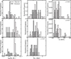 |
Fig. A.1. Normalized distributions of stellar mass as log(M★/M⊙), stellar velocity dispersion (σ★), and effective radius (Re, ★) for observed and simulated galaxies at the three distinctive redshift bins in this study: z = 0.0, z = 0.3, and z = 0.7. Observed data are shown in open histograms and simulated data in grey filled ones. The observational stellar velocity dispersion at z = 0.7 is omitted due to the lack of available measurements in the VIPERS dataset. |
Sample selection across redshift bins (z = 0.0, 0.3, 0.7 and 2.0) and their associated properties.
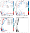 |
Fig. A.2. Stellar mass and size assembly of simulated compact galaxies at four redshifts: z = 0 (upper left), z = 0.3 (upper right), z = 0.7 (lower left), and z = 2 (lower right). Each panel displays the evolution of stellar mass fraction and effective radius over time. All panels are color-coded by the stellar mass accreted since z = 2, except for the z = 2 panel, which remains uncolored. The vertical dashed black line marks z = 2, while the dashed purple line indicates the redshift corresponding to each sample. The horizontal grey line denotes the 90% stellar mass fraction threshold at the given redshift. |
All Tables
Sample selection across redshift bins (z = 0.0, 0.3, 0.7 and 2.0) and their associated properties.
All Figures
|
Fig. 1. Stellar mass–size relation across redshift bins. All TNG50 subhalos are shown as light gray circles in the background, while selected compact subhalos are represented by dark gray circles. Observational CMGs from the different samples are indicated with white diamond markers. The solid black lines follow the mass–size relation from van der Wel et al. (2014), while the dashed gray lines highlight the selection region for the simulated sample (Re < 2 kpc, log Σ1.5 > 10.3 dex). |
| In the text | |
|
Fig. 2. Example of the selected sample of compact TNG50 simulated (left column) and observed (right column) galaxies across redshift bins: z = 0 (top row), z = 0.3 (middle row), and z = 0.7 (bottom row). Observed galaxies include NGC 1277 (top-right, HST ACS/WFC instrument), Spiniello et al. 2024 (middle-right), and VIPERS (bottom-right). |
| In the text | |
|
Fig. 3. Number density of CMGs as a function of redshift, in units of co-moving Mpc−3. The black line and markers represent the TNG50 CMGs from this work. Colored lines and markers correspond to observational estimates from VIPERS (Lisiecki et al. 2023) in red, Scognamiglio et al. (2020) in orange, Damjanov et al. (2014) in green, van der Wel et al. (2014) in purple, Barro et al. (2013) in blue, and Ferré-Mateu et al. (2017) in dark green for the local relics, and magenta for Grèbol-Tomàs et al. (2023) compacts. Simulated CMGs show an increasing number density with redshift, consistent with models predicting more compact objects in the early Universe. A similar trend is seen in the observational data. |
| In the text | |
|
Fig. 4. Stellar mass assembly for the simulated and observed samples at z = 0. The upper panel shows the stellar mass fraction over time for each compact subhalo selected from TNG50, color-coded by the stellar mass growth fraction since z = 2. The lower panel shows the stellar mass assembly over time for the MaNGA compact galaxies of Grèbol-Tomàs et al. (2023), color-coded by group: blue represents Groups B and C, which show extended and/or late SFHs; red represents galaxies in their Group A, which exhibit early and rapid formation (and thus negligible accretion after z = 2); dark red indicates extreme cases, where the galaxy is fully assembled early on (with < 10% accreted material). In both panels, the dashed vertical black line indicates z = 2 and the dashed horizontal gray line indicates the stellar mass fraction of 90%. |
| In the text | |
|
Fig. 5. Stellar mass–stellar velocity dispersion relations for simulated and observed galaxies in the different redshift bins. The dashed black line represents the median σ★ for all TNG50 quiescent subhalos, while the solid black line corresponds to the Zahid et al. (2016) relation across all redshifts. All TNG50 subhalos are shown as gray dots, with the compact sample color-coded by their mass growth since z = 2 (except for the final bin, which is considered he starting point and is therefore left uncolored). Observational data are represented by diamonds, color-coded as follows: dark red for the extreme relics (e.g., extreme cases of group A for MaNGA, DoR > 0.7 for INSPIRE); red for relics (remaining group A of MaNGA and INSPIRE galaxies with 0.5 < DoR < 0.7); and blue for the non-relic group (classes B and C of MaNGA, DoR < 0.5 for INSPIRE). |
| In the text | |
|
Fig. 6. Stellar mass – total stellar metallicity for simulated and observed galaxies. Symbols and colors are as in Fig. 5. A shift of −0.2 dex was applied to the stellar metallicities of simulated subhalos following Nelson et al. (2019). The dashed black line indicates the median stellar metallicity of quiescent subhalos in TNG50. Shaded regions correspond to the local stellar metallicity relations from Gallazzi et al. (2005); the solid black line follows Gallazzi et al. (2005) for z = 0 and z = 0.3, and Gallazzi et al. (2014) for z = 0.7. Observed relics are more metal-rich than other compact galaxies, deviating from the local mass–metallicity relation, while simulated compact galaxies are consistently more metal-rich than the quiescent population, independent of their SFHs. |
| In the text | |
|
Fig. 7. Deviation of stellar metallicity from the simulated quiescent median relation as a function of stellar mass for compact galaxies at different redshifts. Each point represents a galaxy, color-coded by redshift. The Δ dex values correspond to the offset from the running median of the quiescent population at the same redshift. The dashed gray line marks Δ dex = 0, indicating no deviation from the reference relation. Compact galaxies at all redshifts tend to be more metal-rich than typical quiescent systems at the same mass, with the most pronounced offsets seen at lower redshifts. |
| In the text | |
|
Fig. A.1. Normalized distributions of stellar mass as log(M★/M⊙), stellar velocity dispersion (σ★), and effective radius (Re, ★) for observed and simulated galaxies at the three distinctive redshift bins in this study: z = 0.0, z = 0.3, and z = 0.7. Observed data are shown in open histograms and simulated data in grey filled ones. The observational stellar velocity dispersion at z = 0.7 is omitted due to the lack of available measurements in the VIPERS dataset. |
| In the text | |
|
Fig. A.2. Stellar mass and size assembly of simulated compact galaxies at four redshifts: z = 0 (upper left), z = 0.3 (upper right), z = 0.7 (lower left), and z = 2 (lower right). Each panel displays the evolution of stellar mass fraction and effective radius over time. All panels are color-coded by the stellar mass accreted since z = 2, except for the z = 2 panel, which remains uncolored. The vertical dashed black line marks z = 2, while the dashed purple line indicates the redshift corresponding to each sample. The horizontal grey line denotes the 90% stellar mass fraction threshold at the given redshift. |
| In the text | |
Current usage metrics show cumulative count of Article Views (full-text article views including HTML views, PDF and ePub downloads, according to the available data) and Abstracts Views on Vision4Press platform.
Data correspond to usage on the plateform after 2015. The current usage metrics is available 48-96 hours after online publication and is updated daily on week days.
Initial download of the metrics may take a while.