| Issue |
A&A
Volume 704, December 2025
|
|
|---|---|---|
| Article Number | A214 | |
| Number of page(s) | 12 | |
| Section | Stellar structure and evolution | |
| DOI | https://doi.org/10.1051/0004-6361/202555535 | |
| Published online | 12 December 2025 | |
Frequency evolution of pulsar emission
Further evidence for the fan beam model
1
National Astronomical Research Institute of Thailand (Public Organization), 260 M.4, Donkaew, Maerim, Chiang Mai 50180, Thailand
2
Australia Telescope National Facility, CSIRO, Space and Astronomy, PO Box 76 Epping, NSW 1710, Australia
3
Space Science Division, Naval Research Laboratory, Washington, DC 20375, USA
4
Centre for Astrophysics and Supercomputing, Swinburne University of Technology, PO Box 218 Hawthorn, VIC 3122, Australia
5
School of Physics and Astronomy, University of Southampton, Southampton SO17 1BJ, UK
6
OzGrav: The ARC Centre of Excellence for Gravitational-wave Discovery, VIC 3122, Australia
7
SKAO, ARRC Building, 26 Dick Perry Avenue, Kensington, WA 6151, Australia
8
CSIRO, Space and Astronomy, PO Box 1130 Bentley, WA 6102, Australia
9
Jodrell Bank Centre for Astrophysics, The University of Manchester, Alan Turing Building, Manchester M13 9PL, United Kingdom
★ Corresponding author: This email address is being protected from spambots. You need JavaScript enabled to view it.
Received:
16
May
2025
Accepted:
20
September
2025
Abstract
Aims. We explore frequency-dependent changes in pulsar radio emission by analyzing their profile widths and emission heights, assessing whether the simple radius-to-frequency mapping (RFM) or the fan beam model can describe the data.
Methods. Using wideband (704–4032 MHz) Murriyang (Parkes) observations of over 100 pulsars, we measured profile widths at multiple intensity levels, fit Gaussian components, and used aberration–retardation effects to estimate emission altitudes. We compared trends in width evolution and emission height with a fan beam model.
Results. Similar to other recent studies, we find that while many pulsars show profiles narrowing with increasing frequency, a substantial fraction show the reverse. The Gaussian decomposition of the profiles reveals that the peak locations of the components vary little with frequency. However, the component widths do, in general, narrow with increasing frequency. This argues that propagation effects are responsible for the width evolution of the profiles rather than emission height. Overall, the evolution of the emission height with frequency is unclear and clouded by the assumptions in the model. Spin-down luminosity correlates weakly with profile narrowing but not with emission height.
Conclusions. The classic picture where pulsars emit at a single emission height that decreases with increasing observing frequency cannot explain the diversity in behavior observed here. Instead, pulsar beams likely originate from extended regions at multiple altitudes, with fan beam or patchy structures dominating their frequency evolution. Future models must incorporate realistic plasma physics and multi-altitude emission to capture the range of pulsar behaviors.
Key words: polarization / pulsars: general
© The Authors 2025
 Open Access article, published by EDP Sciences, under the terms of the Creative Commons Attribution License (https://creativecommons.org/licenses/by/4.0), which permits unrestricted use, distribution, and reproduction in any medium, provided the original work is properly cited.
This article is published in open access under the Subscribe to Open model. This email address is being protected from spambots. You need JavaScript enabled to view it. to support open access publication.
1. Introduction
It is a well-established idea that the profiles of radio pulsars are narrower at higher radio frequencies (Cordes 1978). This trend is exemplified by pulsars such as PSR B1133+16, where the two components of its profile move closer together as the observing frequency increases (Hassall et al. 2012). Empirically, Thorsett (1991) quantified the frequency evolution of the component separations with a power law. We generalize their relation as follows:
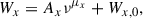 (1)
(1)
where Wx represents the profile width at x% of the peak intensity, ν is the observing frequency, μx characterizes the frequency scaling, and Wx,0 represents the asymptotic width. Multi-frequency data for tens of pulsars analyzed in the 1990s can be fit by the Thorsett relation, seemingly confirming the general narrowing of profile width at high frequencies (e.g., Xilouris et al. 1996; Kijal & Gil 1998; Mitra & Rankin 2002). The frequency-dependent profile evolution is referred to as “radius-to-frequency mapping” (RFM) in the literature and is interpreted as meaning that high-frequency radio emission arises close to the neutron star surface, whereas the low-frequency counterpart originates higher in the magnetosphere. This is due to the fact that the emission cone opening angle increases with altitude.
With a larger sample of pulsars available by 2010, it became obvious that not all pulsars conform to this idea. Chen & Wang (2014) analyzed 150 pulsars and found that ∼54% showed a significant profile narrowing at high ν, but a sizable fraction (∼19%) exhibited broadening at high frequencies, with the rest showing little change. Similarly, Posselt et al. (2021) investigated profile width evolution with frequency for 762 pulsars, revealing that many pulsars exhibit width broadening at higher frequencies, contrary to expectations. Such broadening trends cannot be explained by the simplistic RFM picture.
An alternative fan beam model has emerged to address these issues (e.g., Dyks et al. 2010; Dyks & Rudak 2015; Wang et al. 2014; Dyks & Pierbattista 2015). Unlike the traditional nested cone model, the fan beam model explains profiles as arising from structured, azimuthally elongated beams rather than symmetric concentric rings. The emission consists of elongated streams or fan-like beams of radiation from plasma flowing along specific magnetic field lines, creating a pattern of emission that resembles spokes on a wheel when viewed along the pulsar’s magnetic axis (see, e.g., Fig. 2 in Dyks & Rudak 2015).
Dyks & Pierbattista (2015) argued that the observed peak separation ratio (RW) in pulsar profiles is not consistent with the conal model but is well explained by the fan beam model. They analyzed pulsar profiles with four and five components and measured the separations between these components. They found that the conal model predicts a narrow, sharply peaked distribution of RW, while the observed data show a broader, flatter distribution. The fan beam model, on the other hand, naturally produces the observed distribution. Oswald et al. (2019) studied PSR B1133+16, the pulsar largely responsible for the RFM model, using single-pulse observations at multiple radio frequencies. By comparing the observed frequency-dependent profile broadening with simulations, they demonstrated that profile widening at lower frequencies is more consistent with azimuthally elongated emission patches rather than simple nested cones. The fan beam model therefore serves as an alternative for statistical distributions of peak separations, frequency-dependent broadening, and single-pulse characteristics.
In this paper we measure profile width and emission height evolution across frequencies from 704 MHz to 4.032 GHz. In Section 2 we describe our dataset from Murriyang observations. Section 3 outlines our methodology. Section 4 presents our results on profile characteristics and emission heights. In Section 5 we discuss these findings and propose a simple fan beam model. In Section 6 we summarize our conclusions about pulsar emission geometry.
2. Dataset
The pulsars for this project were observed with Murriyang, CSIRO’s Parkes radio telescope, under the auspices of project ID P574. The P574 project in its current form has been observing some 250 pulsars per month since late 2018 (Johnston et al. 2021). Observations are made with the Ultra-Wideband Low (UWL) receiver (Hobbs et al. 2020) operating in the frequency range 704 to 4032 MHz. The data reduction is identical to that described in Sobey et al. (2021) and also used by Oswald et al. (2023). In brief, the dataset we use here consists of flux and polarization calibrated profiles, with 1024 phase bins across the pulse period. The bandwidth of the UWL is divided into eight subbands, with center frequencies 822, 1070, 1420, 1780, 2107, 2766, 3258, and 3810 MHz.
Of the 250 pulsars regularly observed as part of P574, we removed pulsars with a low flux density and those with clear signs of scatter broadening in the lower frequencies. This left a total of 157 pulsars. They are listed in Table A.1 and Table A.2 in the Appendix.
3. Methodology
3.1. Profile widths
We employed three different methods to determine profile widths. First, the profile width was based on the percentage of the peak intensity. The profile width of each subband was measured at 18 intensity levels, ranging from 5% to 90%, of the profile peak (Wx). Linear interpolation was employed to determine profile edges at specified intensity thresholds. The profile width at each frequency was fit with Eq. (1). The curve fitting process utilized scipy.optimize.curve_fit with the initial parameters A = 100 for the amplitude coefficient, μ = 0.0 for the frequency scaling index, and W = 5° for the asymptotic profile width, along with boundary conditions constraining A between 0 and 2000, μ between −5 and 5, and W between 0° and 100°. The implementation required a minimum of four valid data points for each intensity level to ensure reliable fitting results. The fit parameters and their uncertainties were obtained from the covariance matrix output from the fitting procedure.
As we show in Sections 4 and 5, this methodology is flawed when examining the frequency evolution of the profiles. We therefore adopted a different approach that requires multi-Gaussian component fits to the profiles (e.g., Kramer et al. 1994) at each subband. In the second method, we used the maximum component separation that we denote as Wcomp.sep. We first created a template profile by averaging the data in frequency within each subband and then fit the profiles with multiple Gaussian components using a least-squares optimization approach. The fitting process iteratively added Gaussian components until the residuals fell below the off-pulse noise level. The parameters of this template fit were then used as initial conditions to analyze each frequency subband independently, with bounds set to ±20% of the template values. The maximum component separation (Wcomp.sep) of each subband was then fit with the same curve fitting routine scipy.optimize.curve_fit as in the first method. The separation was measured from the center of the component.
Subsequently, in contrast to the approach employed in the second method, we chose to use the width of each individual Gaussian component, denoted as (Wcomp.width). The values of Wcomp.width for all components were fit according to Eq. (1) using a curve fitting routine similar to the previous methods.
These two methods are not without their caveats. Components are almost certainly not Gaussians, and Gaussian fitting can return non-unique solutions. However in the light of any obvious alternative and with the large sample of pulsars under consideration here, these methods appear to be the most robust way to tackle the problem.
3.2. Emission height
We estimated the pulsar emission height using two different methods. The first is a geometric method. The geometric emission height (r90) correlates with the half-opening angle of the emission beam (ρ) and the star’s rotation period (P). This correlation stems from the pulsar’s dipolar magnetic field structure, which leads to the divergence of field lines from the star’s surface. In this case 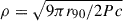 , where c is the speed of light. In turn, ρ can be deduced from the observed profile width, W; the angle between the magnetic and rotation axes, α; and the angle between our line of sight and the rotation axis, ζ. For random samples of the angles α and ζ drawn from a sinusoidal distribution, the W distribution exhibits a peak at 2ρ. We therefore obtained
 (2)
(2)
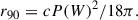
Complementing geometrical methods, the model of Blaskiewicz et al. (1991) enables emission height determination using aberration–retardation effects:
 (3)
(3)
where Δϕ is the phase shift (in degrees) between the profile midpoint and the inflexion of the position angle swing, ϕ0. The determination of ϕ0 comes via the rotating vector model (RVM), originally proposed by Radhakrishnan & Cooke (1969) to describe the observed polarization angle (Ψ) as arising from the projection of a dipolar magnetic field as the pulsar’s emission beam sweeps across an observer’s line of sight. The characteristic polarization angle swing is given by
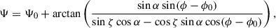 (4)
(4)
where ϕ is the rotational phase and ϕ0 is the phase at which the polarization angle, Ψ, passes through the fiducial plane.
We first performed phase alignment of the subband profiles. Initially, the peak of the profile in subband three was set to phase 180 deg. Then, phase alignment and polarization angle alignment of the pulsar profiles across the subbands were obtained using cross-correlation techniques. The horizontal alignment ensures proper phase alignment across frequency bands, while the vertical alignment corrects for frequency-dependent Faraday rotation effects.
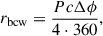
The RVM fitting procedure employed a two-stage optimization approach. Initially, a global fit was performed across all frequency bands using differential evolution to avoid local minima and followed by a local optimization using the L-BFGS-B algorithm. These algorithms were implemented through SciPy’s optimization module (Virtanen et al. 2020). This hybrid approach ensures a robust determination of the key geometric parameters α, β, ϕ0, and ψ0. Parameter uncertainties were estimated using the Hessian matrix. The emission height was derived from the phase shift (Δϕ0) between ϕ0, as determined from the RVM fit, and the center of the profile, measured at 50% of the peak intensity. The uncertainties in the emission heights were propagated from the uncertainties in Δϕ0, which was a combination of the error from the RVM fitting and the profile center with an uncertainty of 1°1 such that 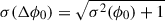 .
.
4. Results
In this section we show figures for one pulsar, PSR J0738–4042, as an illustrative example of the whole sample. We note that although this pulsar has undergone a slow profile change over time (Brook et al. 2014; Zhou et al. 2023; Lower et al. 2023), this does not affect the results shown here. The figures for the other pulsars are available on Zenodo.
4.1. Profile widths
4.1.1. Fraction of peak intensity
The profile width evolution for PSR J0738–4042 is shown in Fig. 1. The profiles are displayed in the left panels, and the different colors correspond to the different subbands. The profile width versus frequency at different intensity percentages is shown in the middle panels. The fit solutions, A, μ, and Wx, 0, are shown in the right panels. The middle panel shows some of the issues inherent in the fitting. The width evolution with frequency at the various percentage cuts depends critically on whether the leading component is included or not. When it is not included, the frequency evolution is essentially flat, A is zero, and μ is undefined. This finding is repeated in many of the pulsars in our sample, particularly those with a large number of components.
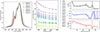 |
Fig. 1. Profile width evolution of PSR J0738–4042. The figure on the left shows the stack of normalized profiles, with the profile peak placed at 180° for each subband. (Middle) The profile width has been measured at varying intensity levels, shown from dark to light colors, in relation to frequency. The dashed lines represent the best-fit solutions of Eq. (1). The resulting parameters as a function of profile intensity level are shown in the right panel. The black, blue, and red lines respectively represent the amplitude, A; the power index, μ; and the y-offset, W0. |
For the 144 pulsars that have σμ < 2°, there are 56 negative and 25 positive values of μ at W10% and 71 negative and 33 positive values of μ at W50%. A two-dimensional contour plot of μ for all the pulsars in the sample as a function of intensity levels is shown in Fig. 2. The counts are weighted by σμ. The figure indicates a tendency toward a negative μ for x < 50%, although approximately 30% of the pulsars in the sample are at positive values of μ. Above x > 50%, the tendency is weaker, indicating that the method breaks down. This is particularly the case for multi-component profiles, where the high-intensity cutoff misses weak components at the profile edges. Our findings are in agreement with the frequency-dependent behaviors previously documented by Chen & Wang (2014) and Posselt et al. (2021). This corroborates the notion that while profile narrowing at higher frequencies remains prevalent, a significant proportion of pulsars manifest contrasting width evolution patterns.
In summary, although historically used and easily applied with tabulated values, a method based on the full width at half maximum (W50), or more generally the full width at x maximum (Wx), is not robust to the choice of x, especially for x > 20%. This result is visible in Fig. 2, which shows that the apparent frequency mapping of the peaks becomes more dispersed as x increases. The apparent width evolution is therefore (in many cases) not dependent on any physics related to diverging field lines or the emission process.
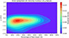 |
Fig. 2. Distribution of frequency evolution index (μ) of profile width measured at different profile intensity level (Wx) for 144 pulsars. The 2D contour map shows the counts weighted by the uncertainty of each data point. |
4.1.2. Component separation
An example of the component fitting for PSR J0738–4042 is shown in Figs. 3 and 4. The Gaussian reconstruction consistently traces the evolution of the component with frequency, with each component maintaining its identity across all subbands. The upper panel of Fig. 5 displays the maximum component separation (Wcomp.sep) as a function of frequency along with the best fit to Eq. (1).
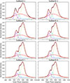 |
Fig. 3. Gaussian component fits of PSR J0738–4042 over eight subbands, showing four individual components (red, blue, purple, and yellow dashed lines). The reconstructed profile is shown with a red dotted line over the profile (black line). |
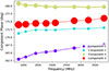 |
Fig. 4. Fitting results of PSR J0738–4042. The y-axis and x-axis represent the Gaussian component location over frequency. The size of the circles represents the widths of the components. |
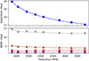 |
Fig. 5. Frequency evolution of the maximum component separation (top) and the component width (bottom) of PSR J0738–4042. The spectral lines are shown with the best-fit solutions of Eq. (1). |
The distribution of μcomp.sep across 128 pulsars is shown in Fig. 6 (left panel). This distribution is approximately symmetric and centered near zero, with a median μcomp.sep value of −0.04 ± 0.48. The uncertainty is the ±1σ percentile of the distribution. The clustering around zero suggests that for many pulsars, the separation between components remains stable across frequency. There is a slight bias toward negative values, suggesting a weak tendency for components to converge with increasing frequency.
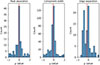 |
Fig. 6. Histogram of μcomp.sep (left), μcomp.width (middle), and μcomp.edge derived from fitting the maximum peak component separation, the individual component widths, and the maximum edge component separation with Eq. (1). (See text for details.) |
4.1.3. Component width
To illustrate the frequency dependence of component widths, we show in Fig. 5 (bottom panel) the widths of the four Gaussian components identified in PSR J0738–4042 (Figs. 3 and 4) as a function of frequency. The distribution of μcomp.width across 128 pulsars is shown in Fig. 6 (middle panel). The distribution is approximately centered near zero, with a median μcomp.width value of −0.10 ± 0.39. This value is more negative than that of the component separation (μcomp.sep = −0.04 ± 0.48), suggesting a stronger tendency for individual components to narrow with increasing frequency. There is a high concentration of components with μcomp.width values near zero.
To confirm the distinction between the evolution of the component width (4.1.3) and the component peak separation (4.1.2), we derived an additional width parameter, Wcomp.edge, which we obtained through a slight modification of Wcomp.sep. Specifically, the position of the edge of an individual Gaussian component was measured at 20% of the peak amplitude of the full profile. For each subband, the largest separation between those edges, i.e., the leftmost and rightmost component edges of the profile, defines the width, Wcomp.edge. Then for each pulsar, the Wcomp.edge of the subbands was fit using Eq. (1)1 following the third method described in Section 3.1.
The results are shown in Fig. 6 (right), which has a median μcomp.edge of −0.26 ± 0.53. The distribution, which has two peaks at ∼0 and ∼ − 1, indicates an even stronger tendency to narrow with increasing observing frequency. In method 1, Wcomp.sep uses the peak position of the outermost Gaussian components, resulting in minimal to no frequency dependence (left). However, for Wcomp.edge, where the boundary is changed to the 20% peak edge position, the distribution considerably shows a stronger frequency dependence in the width evolution (right). These results suggest that the frequency evolution of the profile width is dominated by the frequency evolution of the width of the individual Gaussian components.
4.2. Emission heights
Figure 7 presents the aligned polarization position angle (PPA) sweeps for PSR J0738–4042 across the observed subbands, demonstrating the RVM fits. The evolution of emission heights with frequency for this pulsar is measured as a fraction of the light cylinder radius (RLC).
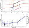 |
Fig. 7. Polarization position angles of PSR J0738–4042 across eight frequency bands. The PPAs are phase-aligned, and position angle swings are overlaid with best-fit RVM curves. The bottom panel shows Δϕ0 (black) and the emission height (blue) against frequency; both appear to increase with frequency. |
Following the criteria by Johnston et al. (2024), the pulsars were classified into three groups based on their Δϕ0: Group –1 for Δϕ0 < −1°, Group 0 for −1° ≤Δϕ0 ≤ 1°, and Group 1 for Δϕ0 > 1°. Based on this classification, our dataset contains 51 pulsars in Group –1, 23 pulsars in Group 0, and 83 pulsars in Group 1. This distribution suggests that the majority of pulsars exhibit a significant positive phase shift (68% for Group 0 and 1), while approximately a third display strong negative shifts (32% for Group –1). The same results were divided into positive and negative trends with frequency, yielding 82 (52%) for the former and 75 (48%) for the latter.
Figure 8 shows how rbcw changes with observing frequency. The top panel plots rbcw in kilometers, while the bottom panel is in units of RLC. Each panel uses a color map to represent the density of data points and is weighted by 1/σ2, where σ is the measurement error. Most pulsars cluster around heights of 100 km or about 0.01 RLC, particularly in the 1200–1800 MHz range. The emission pattern generally shows a symmetric distribution around the 100 km height, with contour lines indicating the emission density constant with frequency.
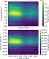 |
Fig. 8. Emission height rbcw vs. ν (1000–3500 MHz) showing weighted density distributions. The panels display emission heights in kilometers (top) and light cylinder radii in RLC (bottom). The color gradient represents the probability density weighted by 1/σ2 of individual measurements, highlighting regions with a higher measurement confidence. |
4.3. Relationship with Ė
Next, we examine how pulsar spin-down luminosity, Ė, relates to various emission properties. Fig. 9 shows the two-dimensional density plot of the profile width evolution parameter, μ, against log (Ė). A weighted linear regression yields μ = −0.16 log(Ė) + 4.8 (coefficient of determination, R2 = 0.5), indicating that pulsars with a higher Ė generally exhibit stronger profile narrowing with increasing frequency. To test the robustness of this trend, we computed the Spearman rank correlation between μ and log10(Ė), obtaining ρ = −0.37, p = 0.22. While the negative ρ suggests a weak-to-moderate inverse monotonic relationship, the high p-value implies that this correlation is not statistically significant. The data are concentrated around μ ≲ 0 and Ė in the range 1033 to 1034 erg/s.
 |
Fig. 9. Error-weighted distribution of μ as a function of |

To further dissect this behavior, we extended our analysis to include the evolution of Gaussian component parameters. In Fig. 10, the component width evolution parameter, μcomp.width, shows a weak positive correlation with log (Ė). The Spearman rank correlation test results in ρ = 0.1511 and the p value = 1.31e−10, indicating a statistically significant but quantitatively small positive monotonic relationship between component width and log Ė. This suggests that pulsars with a higher Ė tend to have marginally wider individual emission components. Although the regression slopes for different frequency subbands are similar, systematic offsets are observed: Lower-frequency subbands generally yield wider component widths compared to higher-frequency subbands at similar Ė values. In contrast, our analysis of the component separation evolution parameter, μcomp.sep, reveals no significant correlation with Ė. This indicates that the spacing between Gaussian components remains largely invariant with respect to the Ė and thus contributes less to the overall frequency evolution of the profile.
 |
Fig. 10. Relationship between the component width (deg) and |

In addition, our analysis of rbcw reveals that the majority of pulsars cluster at moderate heights (200–600 km) over a broad range of Ė (1032–1035 erg/s). In contrast to the trends seen in the profile and component width evolution, rbcw shows no significant dependence on spin-down luminosity. This finding supports earlier suggestions (e.g., Rookyard et al. 2017; Weltevrede & Johnston 2008) that high-Ė pulsars might develop wider profiles not because of a uniformly higher emission altitude but due to emission occurring over an extended range of altitudes.
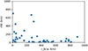 |
Fig. 11. Scatter plot comparing emission altitudes derived from two different methods: r90 in kilometers versus rbcw in kilometers, showing a distribution of values up to 1000 km for both parameters. |
4.4. Data
Table A.1 in the Appendix lists the frequency evolution index (μ) derived from three methods: total profile width at 20% intensity (μ20), component separation (μcomp.sep), and individual component width (μcomp.width), each with uncertainties. Table B.1 presents the group classification by Δϕ0, the slope of height versus frequency, and the correlation between emission height and observing frequency. These data show that many pulsars deviate from the expected trend of decreasing height with frequency, highlighting the complexity of the emission geometry.
5. Discussion
5.1. Profile widths
Our analysis reveals a complex relationship between profile width and observing frequency that cannot be fully captured by traditional width metrics alone (width ∝νa). The majority of pulsars in our sample exhibit a decrease in profile width with increasing frequency, consistent with older studies (e.g., Thorsett 1991; Mitra & Rankin 2002), while a significant subset (∼31%) display an increase in profile width with frequency, consistent with more modern studies (Chen & Wang 2014; Posselt et al. 2023).
We caution that traditional width measurements, such as W10 or W50, fail to reveal the underlying frequency evolution of pulsar profiles, as demonstrated in Fig. 2. This figure supports the Thorsett relationship and RFM to some extent, but it also clearly shows that one might reach contradictory conclusions depending on which intensity level is chosen. These traditional width metrics were established in early studies (Thorsett 1991; Kramer et al. 1994) when pulsar surveys were biased toward low frequencies (typically 400 MHz) and dominated by pulsars that have prominent central components with steep spectral indices. However, our current study at higher frequencies (0.7–4.0 GHz) displays profiles with outrider components that often dominate the profile, necessitating a different approach to the analysis.
A more insightful perspective emerges from analyzing the frequency evolution of the properties of the Gaussian components. We have shown that the separation of the outer components varies only weakly with frequency, whereas the widths of individual components do indeed narrow with increasing frequency. This therefore suggests that the increase in profile width with decreasing frequency is a propagation effect and does not reflect the divergence of the magnetic field lines, or this may result from emission physics (e.g., narrower 1/gamma pencil beamlets).
These findings align with the fan beam model, which predicts minimal frequency evolution along the diverging radial fan beams of emission. In this model, refraction in wave propagation (particularly of the O-mode, Cheng & Ruderman 1979; Barnard & Arons 1986) manifests as widening of individual components. Rather than simply equating low frequency with high emission altitude, our analysis suggests that the relationship between frequency and emission properties is more nuanced and depends on the specific emission geometry and propagation effects. Given these complexities, we recommend that future studies focus on Gaussian component properties rather than width measurements such as W10% that are heavily influenced by spectral characteristics of individual components. Component separation and width measurements provide more physically meaningful parameters that better reflect the underlying emission processes in pulsar magnetospheres.
5.2. Emission height
The results of Section 4 demonstrate an apparent dichotomy in emission height behavior (both rbcw and r90) across frequency bands. Determining rbcw shows that while 75 pulsars (48%) exhibit a decreasing trend with frequency, 82 pulsars (52%) show an apparent increase in emission height with frequency. Fig. 11 shows rbcw versus r90 for our dataset. There is little correlation between the two values, with a Spearman rank-order correlation coefficient of −0.010. This is consistent with the conclusion reached by Mitra & Li (2004), Weltevrede & Johnston (2008) and Desvignes et al. (2019).
When interpreting these results, we must acknowledge the inherent limitations in both methodologies employed to calculate emission heights. First, rbcw depends critically on the accurate identification of the center of the profile, which in our analysis is taken as the midpoint between the leading and trailing edges at 50% of the maximum intensity. This approach introduces potential biases, particularly in asymmetric profiles and those with frequency-dependent component evolution. In addition, the profile center measurement can be skewed due to incomplete beam illumination. Secondly, the geometric height calculations (r90) rely on two critical assumptions: They depend on knowing the pulsar geometry (α and β), which remains poorly constrained for most pulsars (e.g., Everett & Weisberg 2001; Johnston et al. 2023), and they assume the beam is uniformly filled from edge to edge, which may not reflect actual emission patterns (e.g., Lyne & Manchester 1988).
We note that Dyks & Pierbattista (2015) compared fan beam models with the conventional conal models. In the fan beam picture, broadband and coherent emission from secondary relativistic particles forms radially extended sub-beams (Wang et al. 2014; Saha & Dyks 2017; Huang & Wang 2020). When only one or a few flux tubes are active, the fan beam becomes patchy. Dyks & Pierbattista (2015) concluded that the fan beam model gave a better fit to the data.
5.3. Edot
The profiles of high Ė pulsars are different from those of low Ė pulsars. Their components start wider at low frequencies but narrow more quickly as the frequency increases. This pattern arises because high Ė pulsars tend to have smaller magnetospheres. With a smaller magnetosphere, the emission streams lie closer together. This proximity results in a stronger frequency dependence in the stream widths compared to normal pulsars. Other differences include that the emission from high Ė pulsars may come from higher altitudes (Johnston & Weisberg 2006) over a large range of emission heights (Karastergiou & Johnston 2007) and possibly even from outside the conventional polar cap (Weltevrede & Wright 2009; Rookyard et al. 2015). All of this could contribute to profiles that appear wider at low frequencies (as the fan beam streams along the field lines) but experience a sharper contraction with increasing frequency.
This behavior inspires the fan beam model in the next section. Each emission stream changes its width more rapidly with frequency in high Ė pulsars. Their compact magnetospheres produce streams that are more sensitive to frequency-dependent effects. As a result, the individual components narrow faster as the frequency increases.
5.4. A fan beam model
Based on the results outlined in Sections 4.1 and 4.2, we propose a simple fan beam model to explain the data. Fig. 12 illustrates the fan beam model under different assumptions of emission height and observing frequency. Three distinct columns respectively represent high emission height (left), low emission height (middle), and a summation across a continuous range of emission heights (right). In each panel, the line of sight is confined to the lower half of the beam, as indicated by the faint dotted lines filling the bottom region of the circular emission zone. This is because the fan beams stream toward the observer in all parallel line-of-sight directions. The rows represent different observing frequencies, with the top row corresponding to high frequency and the lower rows corresponding to medium frequency and low frequency.
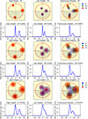 |
Fig. 12. Illustration of a fan beam model. Beam maps (top row in each frequency band) and profiles (bottom row in each frequency band) for three height configurations are presented in separate columns: high height (left), low height (center), and multiple heights (right). From top to bottom, each pair of rows corresponds to a different frequency band: high frequency (HF), medium frequency (MF), and low frequency (LF). The red dashed circle indicates the emission boundary, and the color scale denotes the relative flux intensity. The profile illustrates how amplitude varies with horizontal displacement. (See text for details.) |
A key outcome from this model is that individual emission streams, which are presumed to follow the open magnetic field lines, are broader at low frequency and narrower at high frequency. In contrast to simple geometric models with diverging field lines, the variation in beam width here arises primarily from intrinsic frequency-dependent effects (e.g., refraction or plasma frequency–dependent broadening; McKinnon 1997, Philippov & Kramer 2022) rather than merely from the changing spread of field lines with emission height. Thus, the fan beam interpretation allows for a more nuanced view: The overall beam shape changes modestly with height, but each emission “blob” widens significantly at lower frequencies.
The summation of emission over a continuous range of heights (right column) reproduces, at least qualitatively, the beam patterns observed in more complex pulsar systems, such as the precessing pulsar PSR J1906+0746 (Desvignes et al. 2019), where a streak of emission from the magnetic axis is observed. The beam map retains a characteristic asymmetry and frequency evolution, implying that broadband emission originating over a wide range of altitudes can still manifest clear frequency-dependent beam widths.
An important finding from the data analysis in Section 4.1 is that the profile widths evolve because of changes in the component widths rather than changes in the centroids of the components. As can be seen in Fig. 12, while the overall beam broadens at low frequency, the centroids of the individual emission streams do not shift substantially. In addition, we find that emission heights have virtually no frequency dependence. Within the framework of the model, this arises because the observer sees emission from multiple altitudes at the same time.
Finally, the standard RVM remains largely unaffected by the details of emission height in this fan beam picture. All field lines, regardless of altitude, intersect with the observer’s line of sight at effectively the same magnetic-polar angle. Consequently, the basic RVM sweep is preserved even as the emission streams widen or narrow with frequency, implying that polarization angle constraints on the magnetic geometry remain robust. Overall, the results emphasize that broadband fan beam emission spanning multiple heights can naturally produce wider observed profiles at low frequencies without significantly altering the geometric center or the position-angle swing.
6. Conclusions
We have conducted an investigation into the frequency evolution of pulsar emission geometry using data from the Murriyang (Parkes) telescope. We examined both profile width and emission altitude across a sample of more than 100 pulsars, and our results reveal a more intricate picture than that suggested by the simple RFM model. While many pulsars show the classical trend of narrower profiles and lower emission heights with increasing frequency, a significant subset exhibits the opposite behavior: broadening profiles or higher emission altitudes at higher frequencies.
In particular, we find that measuring the total profile width (e.g., W10 or W50) can obscure the underlying component-level evolution. A more robust view emerges by fitting and tracking individual Gaussian components. Most pulsars do not show large shifts in the centroids of these components; instead, the component widths themselves evolve strongly with frequency. This suggests that the radiation is not simply emitted from a single well-defined conal boundary but may instead arise from fan-like streams whose intrinsic width and intensity vary with observing frequency.
Our measured emission heights, based on aberration–retardation methods, reveal no single, universal pattern. We point out that the assumptions inherent in the method largely obscure the true picture. Moreover, we find no clear correlation between emission altitude and spin-down luminosity (Ė), even though pulsars with a larger Ė show more pronounced frequency evolution in their profile widths. Together, these observations imply that pulsar radio emission arises from a broad, complex region within the magnetosphere, rather than from a thin discrete layer. It is recommended that future research explore the potential of simultaneous multi-frequency single-pulse data (e.g., Oswald et al. 2019; Johnston et al. 2024; Mitra et al. 2024) in order to collect more evidence of the beam geometry.
Data availability
The pulsar data are available to download via the CSIRO Data Access Portal (https://data.csiro.au/). Figures for individual pulsars, similar to those described for PSR J0738–4042 in Section 4, can be found at https://doi.org/10.5281/zenodo.16308954.
An uncertainty of 1° is a conservative estimate based on 1024 bin pulse profiles.
Acknowledgments
This work is supported by the Fundamental Fund of Thailand Science Research and Innovation (TSRI) through the National Astronomical Research Institute of Thailand (Public Organization) (FFB680072/0269). Murriyang, the Parkes radio telescope, is part of the Australia Telescope National Facility (https://ror.org/05qajvd42) which is funded by the Australian Government for operation as a National Facility managed by CSIRO. We acknowledge the Wiradjuri people as the traditional owners of the Observatory site. MEL is supported by an Australian Research Council (ARC) Discovery Early Career Research Award DE250100508. Work at NRL is supported by NASA.
References
- Barnard, J. J., & Arons, J. 1986, ApJ, 302, 138 [NASA ADS] [CrossRef] [Google Scholar]
- Blaskiewicz, M., Cordes, J. M., & Wasserman, I. 1991, ApJ, 370, 643 [Google Scholar]
- Brook, P. R., Karastergiou, A., Buchner, S., et al. 2014, ApJ, 780, L31 [Google Scholar]
- Chen, J. L., & Wang, H. G. 2014, ApJ, 797, 31 [Google Scholar]
- Cheng, A. F., & Ruderman, M. 1979, ApJ, 229, 348 [NASA ADS] [CrossRef] [Google Scholar]
- Cordes, J. M. 1978, ApJ, 222, 1006 [NASA ADS] [CrossRef] [Google Scholar]
- Desvignes, G., Kramer, M., Lee, K., et al. 2019, Science, 365, 1013 [Google Scholar]
- Dyks, J., & Pierbattista, M. 2015, MNRAS, 454, 2216 [Google Scholar]
- Dyks, J., & Rudak, B. 2015, MNRAS, 446, 2505 [Google Scholar]
- Dyks, J., Rudak, B., & Demorest, P. 2010, MNRAS, 401, 1781 [NASA ADS] [CrossRef] [Google Scholar]
- Everett, J. E., & Weisberg, J. M. 2001, ApJ, 553, 341 [NASA ADS] [CrossRef] [Google Scholar]
- Hassall, T. E., Stappers, B. W., Hessels, J. W. T., et al. 2012, A&A, 543, A66 [NASA ADS] [CrossRef] [EDP Sciences] [Google Scholar]
- Hobbs, G., Manchester, R. N., Dunning, A., et al. 2020, PASA, 37 [Google Scholar]
- Huang, W. J., & Wang, H. G. 2020, ApJ, 905, 144 [Google Scholar]
- Johnston, S., & Weisberg, J. M. 2006, MNRAS, 368, 1856 [NASA ADS] [CrossRef] [Google Scholar]
- Johnston, S., Sobey, C., Dai, S., et al. 2021, MNRAS, 502, 1253 [CrossRef] [Google Scholar]
- Johnston, S., Kramer, M., Karastergiou, A., et al. 2023, MNRAS, 520, 4801 [Google Scholar]
- Johnston, S., Mitra, D., Keith, M. J., Oswald, L. S., & Karastergiou, A. 2024, MNRAS, 530, 4839 [Google Scholar]
- Karastergiou, A., & Johnston, S. 2007, MNRAS, 380, 1678 [NASA ADS] [CrossRef] [Google Scholar]
- Kijal, J., & Gil, J. 1998, MNRAS, 299, 855 [NASA ADS] [CrossRef] [Google Scholar]
- Kramer, M., Wielebinski, R., Jessner, A., Gil, J. A., & Seiradakis, J. H. 1994, A&AS, 107, 515 [NASA ADS] [Google Scholar]
- Lower, M. E., Johnston, S., Karastergiou, A., et al. 2023, MNRAS, 524, 5904 [Google Scholar]
- Lyne, A. G., & Manchester, R. N. 1988, MNRAS, 234, 477 [NASA ADS] [CrossRef] [Google Scholar]
- McKinnon, M. 1997, ApJ, 475, 763 [Google Scholar]
- Mitra, D., & Li, X. H. 2004, A&A, 421, 215 [NASA ADS] [CrossRef] [EDP Sciences] [Google Scholar]
- Mitra, D., & Rankin, J. M. 2002, ApJ, 577, 322 [NASA ADS] [CrossRef] [Google Scholar]
- Mitra, D., Basu, R., & Melikidze, G. I. 2024, ApJ, 974, 254 [Google Scholar]
- Oswald, L., Karastergiou, A., & Johnston, S. 2019, MNRAS, 489, 310 [NASA ADS] [CrossRef] [Google Scholar]
- Oswald, L. S., Johnston, S., Karastergiou, A., et al. 2023, MNRAS, 520, 4961 [Google Scholar]
- Philippov, A., & Kramer, M. 2022, Ann. Rev. Astr. Ap., 60, 495 [Google Scholar]
- Posselt, B., Karastergiou, A., Johnston, S., et al. 2021, MNRAS, 508, 4249 [NASA ADS] [CrossRef] [Google Scholar]
- Posselt, B., Karastergiou, A., Johnston, S., et al. 2023, MNRAS, 520, 4582 [NASA ADS] [CrossRef] [Google Scholar]
- Radhakrishnan, V., & Cooke, D. J. 1969, Astrophys. Lett., 3, 225 [NASA ADS] [Google Scholar]
- Rookyard, S. C., Weltevrede, P., & Johnston, S. 2015, MNRAS, 446, 3367 [NASA ADS] [CrossRef] [Google Scholar]
- Rookyard, S. C., Weltevrede, P., Johnston, S., & Kerr, M. 2017, MNRAS, 464, 2018 [Google Scholar]
- Saha, L., & Dyks, J. 2017, MNRAS, 467, 2529 [Google Scholar]
- Sobey, C., Johnston, S., Dai, S., et al. 2021, MNRAS, 504, 228 [NASA ADS] [CrossRef] [Google Scholar]
- Thorsett, S. E. 1991, ApJ, 377, 263 [NASA ADS] [CrossRef] [Google Scholar]
- Virtanen, P., Gommers, R., Oliphant, T. E., et al. 2020, Nat. Methods, 17, 261 [Google Scholar]
- Wang, H. G., Pi, F. P., Zheng, X. P., et al. 2014, ApJ, 789, 73 [NASA ADS] [CrossRef] [Google Scholar]
- Weltevrede, P., & Johnston, S. 2008, MNRAS, 391, 1210 [NASA ADS] [CrossRef] [Google Scholar]
- Weltevrede, P., & Wright, G. 2009, MNRAS, 395, 2117 [NASA ADS] [CrossRef] [Google Scholar]
- Xilouris, K. M., Kramer, M., Jessner, A., Wielebinski, R., & Timofeev, M. 1996, A&A, 309, 481 [NASA ADS] [Google Scholar]
- Zhou, S. Q., Gügercinoğlu, E., Yuan, J. P., et al. 2023, MNRAS, 519, 74 [Google Scholar]
Appendix A: Results from Section 4.1.
Resulting frequency evolution parameters for profile widths.
Resulting frequency evolution parameters for profile widths (continued).
Appendix B: Results from Section 4.2.
Resulting emission height behavior of individual pulsars.
All Tables
All Figures
|
Fig. 1. Profile width evolution of PSR J0738–4042. The figure on the left shows the stack of normalized profiles, with the profile peak placed at 180° for each subband. (Middle) The profile width has been measured at varying intensity levels, shown from dark to light colors, in relation to frequency. The dashed lines represent the best-fit solutions of Eq. (1). The resulting parameters as a function of profile intensity level are shown in the right panel. The black, blue, and red lines respectively represent the amplitude, A; the power index, μ; and the y-offset, W0. |
| In the text | |
|
Fig. 2. Distribution of frequency evolution index (μ) of profile width measured at different profile intensity level (Wx) for 144 pulsars. The 2D contour map shows the counts weighted by the uncertainty of each data point. |
| In the text | |
|
Fig. 3. Gaussian component fits of PSR J0738–4042 over eight subbands, showing four individual components (red, blue, purple, and yellow dashed lines). The reconstructed profile is shown with a red dotted line over the profile (black line). |
| In the text | |
|
Fig. 4. Fitting results of PSR J0738–4042. The y-axis and x-axis represent the Gaussian component location over frequency. The size of the circles represents the widths of the components. |
| In the text | |
|
Fig. 5. Frequency evolution of the maximum component separation (top) and the component width (bottom) of PSR J0738–4042. The spectral lines are shown with the best-fit solutions of Eq. (1). |
| In the text | |
|
Fig. 6. Histogram of μcomp.sep (left), μcomp.width (middle), and μcomp.edge derived from fitting the maximum peak component separation, the individual component widths, and the maximum edge component separation with Eq. (1). (See text for details.) |
| In the text | |
|
Fig. 7. Polarization position angles of PSR J0738–4042 across eight frequency bands. The PPAs are phase-aligned, and position angle swings are overlaid with best-fit RVM curves. The bottom panel shows Δϕ0 (black) and the emission height (blue) against frequency; both appear to increase with frequency. |
| In the text | |
|
Fig. 8. Emission height rbcw vs. ν (1000–3500 MHz) showing weighted density distributions. The panels display emission heights in kilometers (top) and light cylinder radii in RLC (bottom). The color gradient represents the probability density weighted by 1/σ2 of individual measurements, highlighting regions with a higher measurement confidence. |
| In the text | |
|
Fig. 9. Error-weighted distribution of μ as a function of |
| In the text | |
|
Fig. 10. Relationship between the component width (deg) and |
| In the text | |
|
Fig. 11. Scatter plot comparing emission altitudes derived from two different methods: r90 in kilometers versus rbcw in kilometers, showing a distribution of values up to 1000 km for both parameters. |
| In the text | |
|
Fig. 12. Illustration of a fan beam model. Beam maps (top row in each frequency band) and profiles (bottom row in each frequency band) for three height configurations are presented in separate columns: high height (left), low height (center), and multiple heights (right). From top to bottom, each pair of rows corresponds to a different frequency band: high frequency (HF), medium frequency (MF), and low frequency (LF). The red dashed circle indicates the emission boundary, and the color scale denotes the relative flux intensity. The profile illustrates how amplitude varies with horizontal displacement. (See text for details.) |
| In the text | |
Current usage metrics show cumulative count of Article Views (full-text article views including HTML views, PDF and ePub downloads, according to the available data) and Abstracts Views on Vision4Press platform.
Data correspond to usage on the plateform after 2015. The current usage metrics is available 48-96 hours after online publication and is updated daily on week days.
Initial download of the metrics may take a while.