| Issue |
A&A
Volume 704, December 2025
|
|
|---|---|---|
| Article Number | A302 | |
| Number of page(s) | 17 | |
| Section | Cosmology (including clusters of galaxies) | |
| DOI | https://doi.org/10.1051/0004-6361/202556045 | |
| Published online | 18 December 2025 | |
CHEX-MATE: Towards a consistent universal pressure profile and cluster mass reconstruction
1
IRAP, CNRS, Université de Toulouse, CNES, UT3-UPS, Toulouse, France
2
Université Paris-Saclay, Université Paris Cité, CEA, CNRS, AIM, 91191 Gif-sur-Yvette, France
3
Université Grenoble Alpes, CNRS, LPSC-IN2P3, 53, Avenue des Martyrs, 38000 Grenoble, France
4
Université Paris-Saclay, CNRS, Institut d’Astrophysique Spatiale, 91405 Orsay, France
5
INAF, Istituto di Astrofisica Spaziale e Fisica Cosmica di Milano, Via A. Corti 12, 20133 Milano, Italy
6
Dipartimento di Fisica, Università degli studi di Roma Tor Vergata, Via della Ricerca Scientifica 1, I-00133 Roma, Italy
7
INFN, Sezione di Roma ‘Tor Vergata’, Via della Ricerca Scientifica, 1, 00133 Roma, Italy
8
Dipartimento di Fisica, Sapienza Universitá di Roma, Piazzale Aldo Moro 5, I-00185 Rome, Italy
9
Michigan State University (MSU) – Dept of Physics and Astronomy, 567 Wilson Road, East Lansing, Michigan 48824, USA
10
Department of Astronomy, University of Geneva, Ch. d’Ecogia 16, CH-1290 Versoix, Switzerland
11
INAF - Osservatorio di Astrofisica e Scienza dello Spazio di Bologna, Via Piero Gobetti 93/3, I-40129 Bologna, Italy
12
INFN, Sezione di Bologna, Viale Berti Pichat 6/2, I-40127 Bologna, Italy
13
Department of Physics, Informatics and Mathematics, University of Modena and Reggio Emilia, 41125 Modena, Italy
14
Dipartimento di Fisica e Astronomia (DIFA), Alma Mater Studiorum – Universitá di Bologna, Via Gobetti 93/2, 40129 Bologna, Italy
15
Istituto Nazionale di Astrofisica – Istituto di Radioastronomia (IRA), Via Gobetti 101, 40129 Bologna, Italy
16
IJCLab, Université Paris-Saclay, CNRS/IN2P3, IJCLab, 91405 Orsay, France
17
Jodrell Bank Centre for Astrophysics, Department of Physics and Astronomy, The University of Manchester, Manchester M13 9PL, UK
18
Department of Physics, Korea Advanced Institute of Science and Technology (KAIST), 291 Daehak-ro, Yuseong-gu, Daejeon 34141, Republic of Korea
19
Center for Astrophysics | Harvard & Smithsonian, 60 Garden Street, Cambridge, MA 02138, USA
20
HH Wills Physics Laboratory, University of Bristol, Bristol, UK
21
IRFU, CEA, Université Paris-Saclay, 91191 Gif-sur-Yvette, France
22
INFN-Sezione di Genova, Via Dodecaneso 33, 16146 Genova, Italy
23
INAF, Osservatorio Astronomico di Trieste, Via Tiepolo 11, I-34131 Trieste, Italy
24
IFPU, Institute for Fundamental Physics of the Universe, Via Beirut 2, 34014 Trieste, Italy
25
Department of Physics; University of Michigan, Ann Arbor, MI 48109, USA
26
California Institute of Technology, 1200 East California Boulevard, Pasadena, CA, USA
★ Corresponding author: This email address is being protected from spambots. You need JavaScript enabled to view it.
Received:
20
June
2025
Accepted:
17
October
2025
Abstract
In a self-similar paradigm of structure formation, the thermal pressure of the hot intra-cluster gas follows a universal distribution, once the profile of each cluster is normalised based on the proper mass and redshift dependencies. The reconstruction of such a universal pressure profile requires an individual estimate of the mass of each cluster. In this context, we present a method to jointly fit, for the first time, the universal pressure profile and individual cluster M500 masses over a sample of galaxy clusters, properly accounting for correlations between the profile shape and amplitude, and masses that scale the individual profiles. We demonstrate the power of the method and show that a consistent exploitation of the universal pressure profile and cluster mass estimates when modelling the thermal pressure in clusters is necessary to avoid biases. In particular, the method, informed by a cluster mass scale, outputs individual cluster masses with the same accuracy and greater precision than input masses. Using data from the Cluster HEritage project with XMM-Newton: Mass Assembly and Thermodynamics at the Endpoint of structure formation (CHEX-MATE), we investigate a sample of ∼25 galaxy clusters spanning mass and redshift ranges of 2 ≲ M500/1014 M⊙ ≲ 14 and 0.07 < z < 0.6.
Key words: galaxies: clusters: intracluster medium / cosmology: observations / X-rays: galaxies: clusters
© The Authors 2025
 Open Access article, published by EDP Sciences, under the terms of the Creative Commons Attribution License (https://creativecommons.org/licenses/by/4.0), which permits unrestricted use, distribution, and reproduction in any medium, provided the original work is properly cited.
This article is published in open access under the Subscribe to Open model. This email address is being protected from spambots. You need JavaScript enabled to view it. to support open access publication.
1. Introduction
Galaxy clusters are formed by the accretion of matter at the nodes of the cosmic web. If a cluster is virialised and its intra-cluster medium (ICM) fully thermalised, the thermal pressure counterbalances the effect of gravitational forces. Since gravity does not have preferred scales, clusters are nearly scaled versions of each other (see e.g. the reviews in Rosati et al. 2002; Voit 2005), and consequently, the thermal pressure distribution in galaxy clusters is universal (in the intermediate radial range) when normalised with respect to mass and redshift (Nagai et al. 2007; Arnaud et al. 2010, hereafter N07 and A10).
Galaxy cluster detection algorithms for millimetre wavelength observations (Melin et al. 2006; Carvalho et al. 2009) and cosmological analyses based on the thermal Sunyaev-Zel’dovich (tSZ) angular power spectrum (Horowitz & Seljak 2017; Salvati et al. 2018; Bolliet et al. 2018) rely on analytical universal pressure profile (UPP) functionals, calibrated beforehand with dedicated observations. The impact on cosmological results of the assumed profile has been shown to be non-negligible, with different choices shifting the cosmological results, both for the tSZ angular power spectrum and cluster number count analyses (Ruppin et al. 2019; Tanimura et al. 2022; Hernández-Martínez et al. 2025; Gallo et al. 2024).
Several studies have characterised the UPP from tSZ and/or X-ray data (Nagai et al. 2007; Arnaud et al. 2010; Planck Collaboration X 2013; Sayers et al. 2013; McDonald et al. 2014; Sayers et al. 2016; Romero et al. 2017; Bourdin et al. 2017; Sanders et al. 2018; Ghirardini et al. 2019; Pointecouteau et al. 2021; He et al. 2021; Melin & Pratt 2023; Sayers et al. 2023). These various studies differ in the employed methods, datasets, and cluster samples, but they all parametrise the thermal pressure distribution following the generalised Navarro-Frenk-White (gNFW) model. In the present work, we also consider the gNFW parametrisation. This model was adopted by Nagai et al. (2007) (and previously suggested by Zhao 1996), based on galaxy cluster observations and simulations. The previously cited studies demonstrated that the pressure distribution in galaxy clusters overall is close to self-similar at intermediate radii, where gravity drives the physical processes. In the core and outskirts, various processes such as accretion shocks, turbulence, and active galactic nuclei (AGN) feedback (Gaspari et al. 2020) introduce deviations from the universal pressure model.
The reconstruction of a UPP over a population (sample) of clusters requires the scaling of individual profiles by a characteristic mass scale (Kaiser 1986), which we adopt here as M5001, following previous studies. This is the mass of a cluster within a sphere of radius R5001. Thus, the shape and cluster-to-cluster scatter of the derived UPP depends on the manner in which the value of M500 is determined (e.g. see Figure 7 in Arnaud et al. 2010). Ideally, the true value of M500 would be utilised, but direct measurements of this true value are not possible from observations. As a result, most studies rely on observational mass proxies, preferably those with minimal scatter and bias. Traditionally, hydrostatic equilibrium (HSE) or cluster weak lensing mass estimates have been employed to scale the individual pressure profiles, which are then used to measure the UPP. Hydrostatic equilibrium and lensing mass estimates are known to be biased and scattered, respectively, with respect to the true masses (see Pratt et al. 2019, for a review). Usually, individual pressure profiles are scaled according to the value of the chosen characteristic mass proxy, and most previous analyses did not propagate uncertainties and biases associated with those mass proxies, leading to potential biases in the inferred UPP. Recently, He et al. (2021) studied the impact of the HSE mass bias on the UPP, while the uncertainties of mass estimates have been propagated to the UPP error budget in Sayers et al. (2023) (hereafter S23).
As we show in this paper, it appears that characteristic mass scales and universal profile shape and amplitude (for the pressure in our case) are strongly correlated. They, therefore, need to be jointly extracted from a given set of observations to properly propagate the uncertainties from the mass proxies into the universal profile. Otherwise, cosmological analyses based on the UPP will underestimate the current uncertainties. At the same time, if a consistent propagation of the bias associated with the masses used to scale the profiles is not performed, the tSZ modelling using the UPP, and subsequently inferred cosmological parameters, will be biased. In the following, we present for the first time a method to jointly fit the UPP and minimally biased individual cluster masses.
We present this work in the framework of the Cluster HEritage project with XMM-Newton: Mass Assembly and Thermodynamics at the Endpoint of structure formation (CHEX-MATE2, CHEX-MATE Collaboration 2021). The CHEX-MATE project is a multi-year XMM-Newton Heritage programme that aims at understanding the interplay of gravitational and non-gravitational processes in galaxy clusters and their impact on cluster mass estimations. The full sample consists of 118 Planck tSZ-selected clusters spanning mass and redshift ranges of 2 ≲ M500/1014 M⊙ ≲ 14 and 0.05 < z < 0.6. This work focuses on a subsample of CHEX-MATE clusters for which data are already available (Sect. 2). In addition to XMM-Newton data, the CHEX-MATE project has multi-wavelength coverage of the sample, including radio, millimetre, optical, and infrared data (CHEX-MATE Collaboration 2021). In this paper, we make use of X-ray and millimetre wavelength observations to extract thermal pressure profiles (Sect. 2.1) and different cluster mass estimates (Sect. 2.2).
The paper is structured as follows. The dataset is presented in Sect. 2. Section 3 describes the thermal pressure model, and Sect. 4 provides details on the implementation of the fitting method. The results from the application of the method to data are given in Sect. 5. Finally, conclusions are drawn in Sect. 6. We assume a flat Λ cold dark matter (ΛCDM) cosmology with H0 = 70 km s−1 Mpc−1 and Ωm = 0.3. Throughout the paper G corresponds to the Newtonian constant of gravitation, H(z) is the Hubble parameter  , and h70 = H0/(70 km/s/Mpc). The logarithm with base 10 is ‘log’ and ‘ln’ refers to the natural logarithm.
2. Dataset
For the present work, we focus on the ‘Data Release 1’ (DR1) subsample of CHEX-MATE clusters presented in Rossetti et al. (2024). Cluster names, redshifts, and ‘Multi-Matched Filtering 3’ (MMF3) masses (see Sect. 2.2) are summarised in Table 1 in Rossetti et al. (2024). The DR1 clusters have been selected to be representative of the full CHEX-MATE sample in terms of mass, redshift, and X-ray morphology. In this section, we present the data used in this work: the individual pressure profiles for the 28 DR1 clusters3 and their M500 mass estimates.
2.1. Pressure profiles
For each cluster, we combined the thermal pressure profiles reconstructed independently from XMM-Newton X-ray data and Planck tSZ data. Such a combination allowed us to cover a large radial range over the individual profiles: the high angular resolution of XMM-Newton enables tracing the core (down to ∼0.03 × R500), and the outskirts are mapped by Planck. In the following, we briefly present the reconstruction of the individual thermal pressure profiles. We note that other approaches can be taken to reconstruct the pressure distribution. For instance, in the CHEX-MATE paper by De Luca et al. (in prep.), a pressure model was fitted jointly to XMM-Newton and Planck observables following the methodology presented in Bourdin et al. (2017) (hereafter B17). However, as shown in Appendix B in Ghirardini et al. (2019) (hereafter G19), both approaches led to compatible results. In Kim et al. (2024), another pressure reconstruction method was introduced: a forward-modelling technique that jointly fit X-ray and tSZ data to infer 3D intracluster gas properties.
2.1.1. XMM-Newton
The reduction of the raw XMM-Newton data was performed using the CHEX-MATE pipeline described in previous studies (Bartalucci et al. 2023; Lovisari et al. 2024; Rossetti et al. 2024; Riva et al. 2024). First, the data were cleaned by removing the flare events and point sources (see Bartalucci et al. 2023, and references therein). Then, centred on the X-ray peaks, projected surface brightness profiles were reconstructed following the steps detailed in Bartalucci et al. (2023). For this paper we considered the azimuthal median surface brightness profiles, and they were converted into emission measure profiles by accounting for the redshift of each cluster and the emissivity in the 0.7 − 1.2 keV band (Arnaud et al. 2002; Bartalucci et al. 2023). Also centred on the X-ray peaks, the projected temperature profiles were extracted following the spectral fitting method presented in Rossetti et al. (2024).
The deprojection of the profiles was performed as summarised in Riva et al. (2024). The vignetting-corrected and background-subtracted emission profiles were deprojected into density profiles with the geometrical deprojection and point spread function (PSF) correction methods from Croston et al. (2006), accounting for the temperature and abundances in each cluster (Pratt & Arnaud 2003). The binning of surface brightness profiles guarantees a constant signal-to-noise (see e.g. Bartalucci et al. 2023) and defines the binning scheme for the density profiles. The 2D temperature profiles were deprojected and PSF-corrected following the non-parametric-like method from Démoclès et al. (2010) and Bartalucci et al. (2018). As shown in Lovisari et al. (2024), De Luca et al. (in prep.), these temperature estimates are robust with respect to the employed pipeline. The binning of the temperature profiles followed the approach adopted in Rossetti et al. (2024) for the CHEX-MATE DR1 sample, with the optimal binning scheme described in Chen et al. (2024).
Finally, assuming
 (1)
(1)
the 3D pressure profile for each cluster was derived from the combination of the deprojected density, ne(r), and the temperature, Te(r), with kB being the Boltzmann constant. By construction, the pressure profiles were reconstructed in the same radial bins from the temperature and the resampled density profiles. The uncertainties on the pressure were propagated through Monte Carlo Gaussian realisations of the temperature and density profiles. The pressure profiles extracted from XMM-Newton data for the 28 clusters in the sample are shown in orange in Fig. 1. To ensure a homogeneous radial coverage over our sample, we only consider XMM-Newton profiles beyond r/R500 = 0.03 (assuming the R500 from MMF3 M500 estimates; see Sect. 2.2). This way we avoid biases in the core that could be introduced by observational or physical effects (signal-to-noise, presence of cool-cores, etc.; see Melin & Pratt 2023, and references therein). The impact of the assumed centre on pressure profile reconstruction is not investigated in this work, but it could introduce systematic shifts in the innermost bins for disturbed systems.
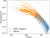 |
Fig. 1. Pressure profiles for the 28 galaxy clusters investigated in this work reconstructed from XMM-Newton (orange) and Planck (blue) data. XMM-Newton data profiles below r/R500 = 0.03 are shaded. These pressure bins are not considered in our analysis (see text). |
2.1.2. Planck
Following the approach established for extracting the Planck tSZ signal in the PACT (Pointecouteau et al. 2021) and X-COP (Ghirardini et al. 2019; Ettori et al. 2019; Eckert et al. 2022) projects, in this work we used the non-public version of the MILCA (Hurier et al. 2013; Planck Collaboration XXII 2016) all-sky y-map (Comptonisation parameter map), reconstructed at a 7 arcmin full-width-half-maximum angular resolution. The pressure profiles were recovered from the y-map following the method presented in Planck Collaboration X (2013) (hereafter P13) and used in subsequent studies (Ghirardini et al. 2019; Ettori et al. 2019; Pointecouteau et al. 2021; Eckert et al. 2022). In summary, Compton-y profiles were computed by azimuthally averaging the signal in concentric annuli in the y-map centred at the X-ray peak of each cluster. Point sources detected in the Planck Catalogue of Compact Sources (Planck Collaboration XXVI 2016) and pixels with signal above a 2.5σ noise level were masked (clipping). The noise level was estimated from the dispersion of the signal in the area between 5 to 10 × θ500 around each cluster. A background zero-level of the y-map (defined from the average signal in [5 − 10]×θ500) was removed from each individual Compton-y profile.
Compton-y profiles were deprojected into 3D thermal pressure profiles by deconvolving from the Planck Gaussian PSF and applying the geometrical deprojection, assuming spherical symmetry and adopting here again the method from Croston et al. (2006). We propagated the contribution of the noise in the y-map and the correlation between the Compton-y profile bins to the final pressure profile covariance matrices as done in previous studies (Planck Collaboration X 2013; Ghirardini et al. 2019; Ettori et al. 2019; Pointecouteau et al. 2021; Eckert et al. 2022). In short, 1000 Compton-y profile realisations computed from 1000 noise realisation y-maps were used to estimate the noise covariance matrix associated with each data Compton-y profile. Each noise covariance matrix was Cholesky decomposed to create 10000 Gaussian realisations centred on each data Compton-y profile. By performing the PSF deconvolution and deprojection of these 10 000 Compton-y profiles, we obtained 10 000 pressure profiles to compute each pressure covariance matrix (Σdata in Eq. (9)). Given the redshift range covered by the sample, some clusters were not fully resolved in the MILCA 7 arcmin y-map, and their pressure profile bins strongly correlate. The individual Planck pressure profiles for the DR1 CHEX-MATE clusters are shown in blue in Fig. 1. Profiles are sampled on a regular grid with bins of width Δr/R500 = 0.25. We limit the profiles to 0.25 − 2.5 × R500.
It should be noted that these Planck pressure profiles are not corrected for the relativistic contribution to the tSZ effect (Pointecouteau et al. 1998; Nozawa et al. 2006). The uncorrected tSZ signal is typically biased by −5 to −15% for Te ∼ 5 − 10 keV galaxy clusters (see Remazeilles et al. 2019; Lee et al. 2020; Perrott 2024, and De Luca et al. in prep.), depending on the temperature of each object. In Fig. 1 we visually perceive a small offset between XMM-Newton and Planck thermal pressure reconstructions within the common radial range. As quantified later in Sect. 5.1, we find a typical ratio of ∼ − 5%. Because the relativistic correction depends on the cluster and the position within each cluster, it is non-trivial to include it within the MILCA maps. As a result, it is beyond the scope of this present work, and tSZ data here are not corrected for relativistic contributions, as in previous studies (e.g. Planck Collaboration X 2013; Ghirardini et al. 2019; Ettori et al. 2019; Pointecouteau et al. 2021; Eckert et al. 2022).
2.2. M500 estimates
As aforementioned, the masses used to scale the pressure are a key element in the reconstruction of the universal profile. In this paper, we make use of different mass estimates.
By ‘MMF3 masses’ we refer to the estimates inferred from the tSZ signal measured by the multi-frequency matched filter MMF3 algorithm on Planck data (Melin et al. 2006; Planck Collaboration XXIX 2014). These are the masses used for the selection of the CHEX-MATE sample (CHEX-MATE Collaboration 2021). For each cluster, the amplitude of the tSZ signal Y500 measured by the MMF3 algorithm was converted into an M500 by applying the scaling relations calibrated beforehand on X-ray data (Planck Collaboration XXVII 2016).
In addition, 24 of the DR1 clusters have ’dynamical mass’ estimates. These were derived from the velocity dispersion of their member galaxies in Sereno et al. (2025). These authors assumed as cluster centres the X-ray peaks from Bartalucci et al. (2023) and adopted the modellings from Navarro et al. (1996), Mamon & Łokas (2005), Diemer & Joyce (2019). Almost independent of the ICM properties, dynamical masses offer an estimate of the mass uncorrelated to the thermal pressure profiles used in this work. As for weak lensing masses, their systematic biases (Gavazzi 2005; Ferragamo et al. 2021) are generally contained down to a percent level (e.g. Ferragamo et al. 2020; Grandis et al. 2021; Aguado-Barahona et al. 2022; Euclid Collaboration: Giocoli et al. 2024; Giocoli et al. 2025; Sommer et al. 2025). Sereno et al. (2025) estimated a bias of  between dynamical and PSZ2 masses (Planck 2nd Sunyaev-Zel’dovich catalogue, Planck Collaboration XXVII 2016). The agreement between the redshift estimates in Sereno et al. (2025) and the redshifts considered in this work is very good: the difference of redshift estimates is Δz/(1 + z) < 0.004 for every cluster. These 24 objects are representative of the CHEX-MATE clusters studied by Sereno et al. (2025) regarding the uncertainties of the individual dynamical masses (see Fig. A.1).
3. Model
In this section, we detail the model used to describe the thermal pressure distribution in clusters. Following Nagai et al. (2007) and Arnaud et al. (2010), we assumed that for each cluster in the sample the pressure profile at the physical radius r is:
 (2)
(2)
with the normalised radius
 (3)
(3)
Here P500 is the normalisation factor of the pressure in physical units. We assumed that it scales with mass and redshift following the self-similar model in Eq. (A.1) in Arnaud et al. (2010), accounting also for a possible deviation from self-similar evolution with mass (Section 3.4 in Arnaud et al. 2010):
![Mathematical equation: $$ \begin{aligned} P_{500}(M_{500}, z)&= \frac{3}{8\pi } \left[ \frac{500 G^{-1/4}}{2} \right]^{4/3} \frac{\mu }{\mu _{\mathrm{e}}} f_{\mathrm{B}} \left[ M_{\mathrm{pivot}} \right]^{ 2/3} \nonumber \\&\times \; H(z)^{8/3} \left[ \frac{M_{500}}{M_{\mathrm{pivot}}} \right]^{\delta }. \end{aligned} $$](/articles/aa/full_html/2025/12/aa56045-25/aa56045-25-eq6.gif) (4)
(4)
Here, the M500 mass is expressed in M⊙ units, and we took the pivot mass Mpivot = 3 × 10¹⁴ M⊙ to be consistent with Arnaud et al. (2010). We considered μ = 0.59, μe = 1.14, and fB = 0.175 for the mean molecular weight, the mean molecular weight per free electron, and the cosmic baryon fraction (defined as fB = Ωb/Ωm), respectively. These values were chosen to be identical to the ones used in Arnaud et al. (2010) and Nagai et al. (2007). More recent estimates of the baryon fraction can be found in the literature (fB = Ωb/Ωm = 0.156 ± 0.003, 0.157 ± 0.004, and 0.157 ± 0.002 from Ωb and Ωm in Planck Collaboration XIII 2016; Planck Collaboration VI 2020; Tristram et al. 2024, respectively). The spread of these values and their uncertainties reflect our current knowledge of fB. These newer constraints by Planck suggest a lower fB than the value we adopted, which shifts the P500 normalisation at the 5 − 10% level. Regarding the molecular weights, we note that Eckert et al. (2019) assumed μ = 0.61 and μe = 1.13, while Ettori et al. (2009) considered μ = 0.600 and μe = 1.155. Molecular weight values depend on the adopted metallicity and, consequently, on the assumed relative abundance table.
In Eq. (4) the scaling of P500 with M500 is determined by the power δ, which in the gravitation-only self-similar scenario takes δ = 2/3. In our framework, δ can also be a free parameter of the model. We assumed the redshift evolution given by the gravitation-only self-similar model, P500 ∝ H(z)8/3. As already investigated in Sayers et al. (2023), Battaglia et al. (2012) and McDonald et al. (2014) for pressure profiles (and in Pratt et al. 2022, for gas density profiles), there could be a deviation from the self-similar evolution with redshift. Since we did not account for it, if present, this would impact our measurement of the evolution of P500 with mass.
The second term in Eq. (2) corresponds to the dimensionless UPP that we aim at fitting. It is meant to describe, on average, the shape of the scaled radial pressure profiles in galaxy clusters. We parametrise ℙ(x) following the gNFW model:
![Mathematical equation: $$ \begin{aligned} \mathbb{P} (x) = \frac{P_0}{(c_{500}x)^{\gamma } \left[1+(c_{500}x)^{\alpha }\right]^{(\beta -\gamma )/\alpha }}, \end{aligned} $$](/articles/aa/full_html/2025/12/aa56045-25/aa56045-25-eq7.gif) (5)
(5)
where P0 is the normalisation constant, c500 the concentration, β and γ are the outer and central power law exponents, respectively, and α gives the slope transition steepness.
Previous studies in the literature (e.g. Ghirardini et al. 2019; Sayers et al. 2023) have shown the need to account for an intrinsic scatter associated with the universal profile. This scatter quantifies the spread about the UPP across the cluster population due to the variety of dynamical states as well as to the impact of non-gravitational processes governing the baryon physics. We assumed a log-normal intrinsic scatter profile σint(x) (see Eq. (10) and Ghirardini et al. 2019; Bartalucci et al. 2023) and chose to parametrise it as a function of the scaled radius x, following
![Mathematical equation: $$ \begin{aligned} \sigma _{\mathrm{int}} (x) = \sigma _1 \exp {\left[- \omega x\right]} + \sigma _0 x, \end{aligned} $$](/articles/aa/full_html/2025/12/aa56045-25/aa56045-25-eq8.gif) (6)
(6)
with σ1, σ0, and ω as the free parameters in the model. In Appendix B we discuss the choice of this particular parametrisation with respect to other options in the literature. We also account for the covariance of the Gaussian process describing the intrinsic scatter with an additional free parameter Lint, as detailed in Sect. 4 (Eq. (11)).
In addition, when combining X-ray and tSZ-based pressure profiles, one must account for a potential systematic discrepancy between them (Kozmanyan et al. 2019, De Luca et al. in prep.). As investigated in Kozmanyan et al. (2019), Ettori et al. (2020a), Wan et al. (2021), multiple factors can be at the origin of such a discrepancy and, in the literature, it is quantified as ℛ or ηT:
 (7)
(7)
We consider the normalisation factor ηT as a free parameter that calibrates the ratio between X-ray and tSZ-based pressure profiles.
In summary, our model contains two types of free parameters, θ:
-
Global parameters or parameters common to all clusters. These are: the power in the P500 − M500 scaling relation (δ); the parameters of the UPP gNFW profile (P0, c500, α, β, γ); the parameters describing the intrinsic scatter (σ1, σ0, ω, and Lint); and the ratio between X-ray and tSZ pressure profiles (ηT).
-
Individual parameters. In particular, we have one mass parameter per galaxy cluster: {M500, 1, ..., M500, n}. In a fixed cosmology and assuming a redshift per cluster, the conversion between M500 and R500 (needed to calculate the x in the model, Eq. (3)) is straightforward1.
In this framework any of the mentioned parameters can be fitted or fixed to a predefined value.
In the literature the power-law exponent in the P500 − M500 scaling relation is often fixed to the self-similar δ0 = 2/3 value (e.g. Ghirardini et al. 2019). Nevertheless, some works (Arnaud et al. 2010; Sayers et al. 2013; He et al. 2021; Sayers et al. 2023) have already studied the deviation from self-similarity, obtaining values that span from δ ∼ δ0 − 0.20 to δ ∼ δ0 + 0.12. According to simulations (Le Brun et al. 2017; Cui et al. 2018), the power should be very close to δ0 = 2/3 but reaching almost δ0 + 0.33 in Le Brun et al. (2017) and δ0 − 0.03 in Cui et al. (2018). In addition, as shown in He et al. (2021), the estimation of δ correlates with the assumed mass scale.
Regarding the intrinsic scatter of the universal profile, we find in the literature studies that jointly fit the scatter and the pressure profile (Sayers et al. 2013; Ghirardini et al. 2019; Sayers et al. 2023) as well as studies that measure a posteriori the spread of the data with respect to the UPP (Arnaud et al. 2010; Bourdin et al. 2017). We here opt for the joint fit.
For the first time compared to other studies, in this paper we allow individual cluster masses to vary during the fit of the UPP. This constitutes the main novelty of the presented approach.
4. Fitting method
In practice, our model assumes that each individual pressure profile Pdata, i (Fig. 1) is well described by a multivariate Gaussian distribution:
![Mathematical equation: $$ \begin{aligned} \mathcal{L} _i = \frac{1}{\sqrt{(2 \pi )^{n_i} |C_i|}} \mathrm{exp}\left[ -\frac{1}{2} (P_{\mathrm{data}, i}- P_{\mathrm{mod}, i})^T C_i^{-1} (P_{\mathrm{data}, i}- P_{\mathrm{mod}, i}) \right], \end{aligned} $$](/articles/aa/full_html/2025/12/aa56045-25/aa56045-25-eq10.gif) (8)
(8)
with ni being the number of data pressure bins for cluster i. In the above equation, Pmod, i(θ) corresponds to the pressure profile model (Eq. (2)), and Ci(θ) is the covariance matrix (Sayers et al. 2013, 2023; Bartalucci et al. 2023) given by:
 (9)
(9)
where  is the covariance of the data pressure profile for the radial bins k and l. In this equation, Σint, i is a matrix that accounts for intrinsic dispersion. Since we consider a log-normal scatter, each diagonal element of Σint, i is defined as
![Mathematical equation: $$ \begin{aligned} \begin{split} \Sigma _{\mathrm{int}, i}^{k, k} (\theta )&= \left[ P_{\mathrm{mod}, i} (r_{i, k}, \theta ) \times \sigma _{\mathrm{int}} (r_{i, k}, \theta ) \right]^2 \\&= \left[ P_{500, i} (\theta ) \; \mathbb{P} (r_{i, k}, \theta ) \times \sigma _{\mathrm{int}} (r_{i, k}, \theta ) \right]^2. \end{split} \end{aligned} $$](/articles/aa/full_html/2025/12/aa56045-25/aa56045-25-eq13.gif) (10)
(10)
Here, P500, i (Eq. (4)), ℙ (Eq. (5)), and σint (Eq. (6)) are functions of the free parameters in the model: θ = {M500, 1, …, M500, n; P0, c500, α, β, γ; δ; ηT; σ1, σ0, ω}. In Eq. (10), ri, k corresponds to the physical radius of the pressure profile for the k-th bin in cluster i.
Pressure profiles are generally thought to be smooth, with neighbouring points correlating with each other. Thus, we introduce a correlation in the intrinsic scatter covariance matrix using a ‘radial basis function’ or ‘squared-exponential’ kernel (as already used, e.g. in Kern & Liu 2021), where the kernel size is defined by the Lint parameter:
![Mathematical equation: $$ \begin{aligned} \Sigma _{\mathrm{int}, i}^{k, l} (\theta ) = \sqrt{\Sigma _{\mathrm{int}, i}^{k, k} \Sigma _{\mathrm{int}, i}^{l, l}} \exp {\left[ - \frac{(x_{i, k} - x_{i, l})^2}{2 L_{\mathrm{int}}^2} \right]}, \end{aligned} $$](/articles/aa/full_html/2025/12/aa56045-25/aa56045-25-eq14.gif) (11)
(11)
with xi, k = ri, k/R500, i and xi, l = ri, l/R500, i following Eq. (3). By considering this covariance kernel for the intrinsic scatter, we assume contiguous pressure bins to be more correlated to each other and no anti-correlations. The Lint parameter quantifies the radial distance between correlated bins, and it allows modelling systematic deviation with respect to the UPP.
Markov chain Monte Carlo (MCMC) sampling was used to fit the free parameters describing the model to the data. Given the large number of parameters that the model can encompass, an efficient fitting method was required. For this reason, we relied on jax-based codes (Bradbury et al. 2018) that enable the automatic differentiation of distributions and, thus, a fast sampling of the posterior probability distribution. We performed the Bayesian inference making use of the no U-turn sampler (NUTS, Hoffman & Gelman 2014), as implemented in the numpyro (Bingham et al. 2019; Phan et al. 2019, 2025) Python library. In the Bayesian framework, our posterior probability distribution of the parameters is a combination of the multivariate Gaussian distribution quantifying the likelihood of the data to satisfy the model and the prior distribution associated with each free parameter. The final likelihood is the product of all the n individual cluster likelihoods:  . Table 1 summarises the priors considered in this work.
Prior distributions for the parameters in the model.
The sampling was performed using ten chains and 103 tuning steps. The number of sampling steps needed to reach convergence typically ranged from ∼104 to ∼105, depending on whether individual cluster masses were fitted or not. We kept the four chains with the highest posterior probability distributions and considered the MCMC chains to have converged when the  condition (Gelman & Rubin 1992; Vehtari et al. 2021) was met.
5. Measuring the universal pressure profile and individual cluster masses
In this section, we present the results obtained by applying the described method to our CHEX-MATE dataset (Sect. 2) for the 24 clusters with available dynamical masses. We considered all the individual cluster M500, i masses as free parameters. This means that, at each step of the fit, both P500 and x values varied, without adapting the number of considered pressure bins at each step. The change was accounted for in the computation of the model at each MCMC step, rather than in the data. A shift in M500 and, consequently, in R500, implies a change in the normalisation of the P(r) pressure profile along the ordinate (Eq. (4)) as well as in the abscissa (r in Eq. (3)), causing the profile to shrink or stretch along both axes. Such a shift in M500 can mimic the effect of a modification in gNFW shape parameters. This means that when pressure profiles are fitted by assuming fixed M500 values, the resulting UPP is directly affected by the considered masses. And as a consequence, the use of inadequate mass estimates leads to incorrect UPP measurements.
Dynamical mass estimates (Sect. 2.2) are ideal priors for the cluster masses in the joint fit of our data pressure profiles: they are expected to be scattered but (almost) unbiased mass estimates (Gavazzi 2005; Ferragamo et al. 2021). Appendix C presents the validation of our method and demonstrates that, if unbiased, even scattered mass estimates are good priors to inform the fit. Moreover, dynamical masses mostly do not correlate with the XMM-Newton and Planck pressure profiles (Sect. 2.1).
Best-fit parameters from the joint fit of pressure profiles assuming dynamical mass priors and for different δ values.
5.1. Joint fit of individual cluster masses and the UPP
By taking Gaussian priors centred on the dynamical masses with their deviation corresponding to the dynamical mass measurement errors (Table 1) as estimated in Sereno et al. (2025), we performed the joint fit of the universal gNFW pressure profile and the individual masses for the 24 clusters in our subsample (see Sect. 2.2). We considered three cases: (1) δ fixed to the self-similar value, (2) δ fixed to 2/3 + 0.12 (as in Arnaud et al. 2010), and (3) δ treated as a free parameter of the model. For the latter, we considered a Gaussian prior distribution centred on the self-similar 2/3 with a standard deviation of 0.2 (Table 1). By investigating these three cases, we studied the impact of the assumed P500 − M500 scaling relation on the UPP. We adopted flat priors for the rest of the parameters (Table 1).
The colour profiles in the top panels in Fig. 2 indicate the normalised individual pressure profiles for our 24 galaxy clusters. They are normalised by the P500, i and R500, i values for the best-fitting M500, i and δ parameters (Table 2). The solid black profiles show the best-fitting gNFW model for each case of δ (parameter values are summarised in Table 2), and below each panel we present the relative difference between the normalised individual profiles and the best-fitting gNFW. The corner plot in Fig. D.1 shows the 1D and 2D posterior distributions for all the fitted parameters, colour-coded as in Fig. 2. Regarding the ratio between X-ray and tSZ data, we obtain for all three cases a best-fit value of ηT ∼ 1.05, consistent with that expected from neglecting tSZ relativistic corrections (Sect. 2.1.2).
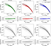 |
Fig. 2. Normalised data pressure profiles, best-fit gNFW models, and their relative difference. Top: Coloured profiles show the individual data pressure profiles (from Fig. 1) for the 24 clusters normalised by the best P500, i and R500, i values when fitting the individual masses with dynamical mass estimates as priors. Green, red, and blue correspond to the fits assuming respectively δ = 2/3, δ = 2/3 + 0.12, and δ as a free parameter. Bottom: Data pressure profiles in grey, normalised by P500, i and R500, i values, with masses fixed in the fit and set to the dynamical mass estimates. The solid black profile in each panel indicates the best-fit gNFW profile for that case, with the dotted profiles showing the fitted intrinsic scatter ℙ(x)exp[±σint(x)]. The dashed profiles in the top (bottom) panels correspond to the best-fit gNFW for the mass-fixed (fitted) cases. |
For what concerns the power law in the P500 − M500 scaling relation, the data prefer a high value of δ = 0.85 when this parameter is allowed to vary freely, in line with Arnaud et al. (2010), Ettori et al. (2020b, 2023). However, the marginalised posterior distribution of δ is in agreement with self-similar evolution. As expected δ mainly correlates with P0 and cluster masses (Fig. D.1). The departure of the best-fit δ from the self-similar expectation could be interpreted as a mass-dependent gas mass fraction  (Ettori et al. 2020b, 2023) and our results suggest an increase in the gas mass fraction with cluster mass (see other recent results in Wicker et al. 2023; Ettori et al. 2023). This trend could be linked to non-gravitational processes that can modify the thermodynamics of the ICM, such as AGN feedback and turbulence (Wittor & Gaspari 2020). The model presented in this work could be extended to directly fit fgas in future applications. It is also worth noting the small impact of the various δ values considered in this work on the rest of the free parameters.
The best-fitting individual cluster masses are presented with respect to the dynamical estimates in the top panel in Fig. 3. Green, red, and blue markers correspond to the masses obtained by assuming different power values in the P500 − M500 scaling relation. We observe that, by construction of the priors, fitted masses are scaled to the dynamical mass scale ( , 1.003 ± 0.494, and 1.031 ± 0.513 for δ = 2/3, 2/3 + 0.12, and δ free cases, respectively), but corrected when informed by the thermal pressure distribution. We stress that in Fig. 3 the error bars of the fitted masses correspond to the standard deviation of the marginalised posterior distribution for each cluster mass parameter. These error bars are not representative of the uncertainties we have on individual masses, since they all strongly correlate with each other. The corner plot in Fig. D.1 illustrates these correlations between the M500, i. Fig. D.2 compares the marginalised posterior distributions of the 24 M500, i parameters to the Gaussian priors assumed for the cluster masses, showing how fitted masses deviate from the considered prior distributions. In the bottom panel in Fig. 3, we compare the fitted masses to the MMF3 estimates. They exhibit strong correlation. On average, their ratio is
  , 1.327 ± 0.228, and 1.356 ± 0.212 (for δ = 2/3, 2/3 + 0.12, and δ free cases, respectively), which is comparable with the bias reported in Sereno et al. (2025). Similarly, when comparing fitted masses to HSE estimates reconstructed from XMM-Newton data, we obtain
  , 1.419 ± 0.321, and 1.447 ± 0.293 for δ = 2/3, 2/3 + 0.12, and δ free cases, respectively.
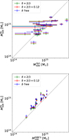 |
Fig. 3. Masses obtained from the joint fit to data by taking Gaussian priors centred on dynamical estimates. We compare the results to the dynamical (top) and MMF3 (bottom) mass estimates. The colour scheme is identical to that in Fig. 2 for the different values of δ. Uncertainties of fitted masses are calculated as the standard deviation of the marginalised posterior distribution for each cluster mass parameter. |
By jointly fitting the UPP and cluster masses, we propagated the uncertainties on the individual masses to the UPP. In addition, we recovered the intrinsic scatter of the pressure profiles, due mainly to the baryon physics and variations in clusters’ dynamical states across our sample, without being impacted by the scatter of the mass estimates used to scale the individual profiles (see Ghirardini et al. 2019; Riva et al. 2024). The shaded profile in Fig. 4 shows the fitted intrinsic scatter profile. We only present the profile obtained from the fit with δ as a free parameter, but the δ = 2/3 and δ = 2/3 + 0.12 cases give fully compatible results (see Fig. D.1). We observe a decreasing trend with radius up to x ∼ 1.2, where the scatter starts to rise again. In the same figure, the dashed profile indicates the scatter of the individual pressure profiles with respect to the UPP (σtot). Grey crosses and circles indicate the statistical uncertainties (σstat, square root of the covariance matrix diagonal) of each individual pressure profile for the XMM-Newton and Planck bins, respectively. We notice that at large radii (beyond x ∼ 0.4) the level of statistical uncertainties prevents us from constraining the underlying intrinsic scatter4: statistical uncertainties are as large as σtot, which explains the very low intrinsic scatter we measure compared to other studies (Fig. B.1). We verified that the same effect is observed when performing the joint fits by modelling the intrinsic scatter using the parametrisation in Eq. (B.1) from Ghirardini et al. (2019), and that fitted M500, i parameters remain consistent. By varying Lint freely in the fit, we measure a correlation length of ∼0.3.
 |
Fig. 4. Scatter of pressure profiles for the 24 clusters in our sample. The shaded area indicates the 16th to 84th percentiles for the intrinsic scatter profile fitted to data pressure profiles (δ free case). The intrinsic scatter may not be reliably constrained beyond x ∼ 0.4. The dashed line indicates the scatter of the individual normalised profiles with respect to the best-fit gNFW model. Statistical uncertainties of the individual pressure profiles are indicated with crosses and circles for the pressure bins corresponding to XMM-Newton and Planck data, respectively. All scatters are given in P500ℙ(x) units. |
We repeated the fits but fixed the cluster masses according to the dynamical estimates in Sereno et al. (2025). The individual normalised pressure profiles and best-fit gNFW profiles are shown in the bottom panels in Fig. 2. Unsurprisingly, given their large scatter, dynamical masses are not suited to scale directly the individual profiles, leading to an overestimation of the intrinsic scatter. On the contrary, by jointly fitting the pressure and masses, we are able to refine the latter and find the masses that scale the pressure profiles the best (top panels in Fig. 2).
Finally, we performed the joint fit of the individual masses and UPP parameters by considering only the XMM-Newton pressure bins (orange profiles in Fig. 1). Given the radially constant and small statistical uncertainty sizes (Fig. 4), we recovered the intrinsic scatter profile shape expected from previous studies (see Fig. B.1). However, the radial extent of XMM-Newton profiles is not large enough to fully constrain the gNFW profile shape and significantly improve on the mass estimates. Consequently, the intrinsic scatter is overestimated by the dispersion of dynamical mass estimates.
Further analyses could try to model the intrinsic scatter in the P500 − M500 scaling relation, as well as the scatter of the fitted masses with respect to the true M500, particularly if mass proxies with small nominal uncertainties are used as priors. The current work presumes those scatters to be zero. Although the impact of the assumed cosmology on the resulting UPP and masses is not assessed in this paper, it directly affects the results through the deprojection of the individual pressure profiles and the definitions of R500 and P500 (Eq. (4)). This impact should be quantified and coherently considered for further use in cosmological analyses.
5.2. Impact of the UPP on the mass determination
In the previous sections (and in Appendix C), we demonstrated the complex degeneracies between the parameters in the model. Here, we further stress the intricate interdependencies between the UPP and cluster masses, by assessing the impact of the UPP shape on the measured masses over a given sample.
We considered various gNFW profiles from the literature (N07, A10, P13, B17, G19, PACT, S23, and Melin & Pratt 2023, hereafter MP23), assuming also the associated values of δ adopted in each of these studies (Table E.1). These eight gNFW profiles are drawn in Fig. E.1. For each case we fixed the given UPP and performed a fit of the individual 24 masses for our clusters. We assumed no intrinsic scatter, and as in Sect. 5.1, adopted Gaussian priors centred on the dynamical mass estimates from Sereno et al. (2025).
The results for the tested gNFW cases, given in Table E.1, are shown in Fig. 5. Violin plots illustrate the best-fit M500 distributions for the 24 clusters, for fits with ηT as a free parameter. The statistical averages of the fitted masses over our sample are shown with circles. Diamonds give the average mass for fits with ηT fixed to 1.05. In the same figure, we present the distribution and average of the best-fit masses from our joint fits with the UPP obtained in Sect. 5.1. Unsurprisingly, the joint fit of the UPP parameters and individual cluster masses performs the best (in particular, for δ = 2/3 and δ free cases) in modelling the data pressure profiles.
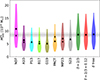 |
Fig. 5. Distribution of the 24 best-fit M500 obtained from the thermal pressure profile fits with ηT free. We present the average mass of the sample for fixed UPPs from the literature, shown with circles and diamonds for the cases where ηT is free in the fit and fixed to ηT = 1.05, respectively. We also show the |

The UPPs we tested were all derived from different samples, with individual cluster pressure profiles normalised with masses obtained under different hypotheses. In N07 and A10, the authors used X-ray-only pressure profiles (together with simulations), while PACT and MP23 studies are based on tSZ-only analyses. The rest of the studies (P13, B17, G19, S23, and this work) combine X-ray and tSZ data. No differentiation between tSZ and X-ray-based results is observed in Fig. 5. Similarly, from the variety of mass and redshift ranges of the samples used in the considered studies, we do not observe any obvious trend that could have pointed towards an evolution of the UPP. In A10, P13, B17, and PACT the provided UPPs were derived by normalising individual pressure profiles with masses estimated from tSZ or X-ray scaling relations. In G19 the authors made use of masses measured from their own HSE mass profiles (based on XMM-Newton and Planck data). By comparison, in MP23 the authors employed the SPT masses (Bleem et al. 2015), renormalised for compatibility with the A10 mass definition, while in N07 the authors assumed Chandra HSE masses. Thus, all of the mentioned UPPs were reconstructed by normalising the individual pressure profiles with tSZ or X-ray-based masses, which are known to be biased low as they do not account for the presence of non-thermal pressure in clusters (Pratt et al. 2019). Contrarily, in S23 cluster masses were obtained from an X-ray scaling relation calibrated using weak lensing masses (Mantz et al. 2016).
The masses we derived over our sample of 24 clusters by assuming the shape of each aforementioned UPP from the literature are also low against those obtained from our joint fit with the UPP and scaling law parameters (green, red, and blue results in Fig. 5). The only exception is N07, who used a sample of relaxed, hot systems (TX > 5 keV), resulting in a peaked and steeper UPP shape (see Fig. E.1) that subsequently biases the associated fitted masses towards higher values. When comparing to N07 (and S23) results one must also bear in mind the temperature cross-calibration difference between Chandra and XMM-Newton (Schellenberger et al. 2015).
We note that when fixing the UPP to the A10 profile, we consistently fall back on the MMF3 masses ( ), even when taking dynamical masses as priors. The MMF3 masses were obtained by measuring the tSZ signal on Planck maps (Sect. 2.2), assuming the A10 parameters (Planck Collaboration XXIX 2014). This is a further coherence-check demonstrating the validity of our method.
In the end, the average relative difference across the cases we tested is −23, −23, and −24% (−30, −30, and −31% when excluding N07) with respect to our best-fit masses for δ = 2/3, δ = 2/3 + 0.12, and δ free cases, respectively. The various average cluster mass scales we derived when fixing the UPPs differ by ∼10 to ∼50%. As seen from the simulations in Appendix C, this stresses the intricate dependence between the mass scale and the UPP. Thus, the consistent use of the cluster mass scale, P500 − M500 scaling relation, and UPP shape are needed to prevent biases in dependent studies, such as the cosmological analysis based on the tSZ angular power spectrum (Horowitz & Seljak 2017; Salvati et al. 2018; Bolliet et al. 2018). In the reconstruction of the UPP from a given sample, the closer the normalising masses are to the true mass scale, the lower the biases on the reconstructed UPP.
Other biases, such as selection effects, also have an impact on the inferred UPP shape and amplitude (e.g. A10). The literature UPPs we tested here have been built upon samples of clusters with different levels of representativity and were not corrected for selection bias effects5. The same stands for our current sample of 24 clusters. The full CHEX-MATE sample, as an actual representative sample of the galaxy cluster population at low redshift and at high mass, accounting for the aforementioned selection bias, is appropriate to conduct such a consistent study of the UPP, the P500 − M500 scaling, and the masses, to determine the ‘absolute mass scale’ of the cluster population.
6. Summary and conclusions
In view of the strong correlation between the UPP shape and the assumed cluster mass scale, we built a framework that enables, for the first time, the joint fit of the UPP and individual cluster masses. The model accounts for the intrinsic scatter of the pressure profile and for a potential systematic difference between thermal pressure profiles reconstructed from X-ray and tSZ data.
We applied the method to 24 CHEX-MATE clusters for which XMM-Newton and Planck thermal pressure profiles and dynamical mass estimates are available. Despite the limitations associated with the small sample size considered in this proof-of-concept paper, the sample is large enough to perform a statistical analysis. By jointly fitting the individual cluster masses and UPP parameters, we were able to: 1) reconstruct the best gNFW model describing the shape of the pressure distribution for this sample; 2) propagate the uncertainties of individual cluster masses to the UPP; and 3) refine the individual cluster masses into low scatter mass estimates.
Finally, we quantified the impact of the assumed UPP shape on the cluster masses measured from the thermal pressure profiles. We confirm the need for a coherent modelling of the pressure. The self-consistent UPP and M500 framework is particularly suitable for tSZ cosmological statistics (e.g. power spectrum and cluster number counts) where mass scaling assumptions propagate into cosmological parameters.
This work establishes the basis for the universal pressure profile analysis that will be carried out with the full CHEX-MATE cluster sample. Further studies will investigate the physical implications outlined in this paper, account for the relativistic correction to the tSZ signal, and explore the impact of consistently modelling the pressure and a full propagation of the uncertainties on the cosmological results.
M500 and R500 are defined as M500 = (4/3)πR5003 × 500ρcrit, where ρcrit(z) = 3H(z)2/(8πG) is the critical density of the Universe at the cluster redshift z. Similarly, we define θ500 as θ500 = R500/DA, with DA being the angular-diameter distance of the cluster.
We excluded PSZ2 G042.81+56.61 and PSZ2 G057.78+52.32 for which XMM-Newton observations include off-set pointings not implemented in the current version of the analysis.
The tight constraints we obtain on σ0, σ1, and ω are an artefact of the chosen parametrisation, which does not allow for a low intrinsic scatter profile as well as large uncertainties.
MP23 corrected for the selection bias of SPT clusters in the South Pole Telescope Sunyaev–Zel’dovich survey (SPT-SZ, Bleem et al. 2015) data.
Acknowledgments
Authors acknowledge the support of the French Agence Nationale de la Recherche (ANR), under grant ANR-22-CE31-0010, and the support of the French National Space Agency (CNES). This research was supported by the International Space Science Institute (ISSI) in Bern, through ISSI International Team project #565 (Multi-Wavelength Studies of the Culmination of Structure Formation in the Universe). S.E., M.S., M.R., H.B., F.D.L., and P.M. acknowledge the financial contribution from the contracts Prin-MUR 2022 supported by Next Generation EU (M4.C2.1.1, n.20227RNLY3 The concordance cosmological model: stress-tests with galaxy clusters). M.S. acknowledges the financial contributions from contract INAF mainstream project 1.05.01.86.10, INAF Theory Grant 2023: Gravitational lensing detection of matter distribution at galaxy cluster boundaries and beyond (1.05.23.06.17). S.E., M.R. acknowledge the financial contribution from the European Union’s Horizon 2020 Programme under the AHEAD2020 project (grant agreement n. 871158). M.D. acknowledges the support of two NASA programs: NASA award 80NSSC19K0116/ SAO SV9-89010 and NASA award 80NSSC22K0476. L.L. acknowledges the financial contribution from the INAF grant 1.05.12.04.01. B.J.M. acknowledges support from STFC grant ST/V000454/1. M.D.P. acknowledges financial support from PRIN-MUR grant 20228B938N ‘Mass and selection biases of galaxy clusters: a multi-probe approach’ funded by the European Union Next generation EU, Mission 4 Component 1 CUP C53D2300092 0006. H.S. acknowledges support by NASA Astrophysics Data Analysis Program (ADAP) Grant 80NSSC21K1571. H.B., F.D.L., and P.M. acknowledge support by the Fondazione ICSC, Spoke 3 Astrophysics and Cosmos Observations. National Recovery and Resilience Plan (Piano Nazionale di Ripresa e Resilienza, PNRR) Project ID CN_00000013 ’Italian Research Center on High-Performance Computing, Big Data and Quantum Computing’ funded by MUR Missione 4 Componente 2 Investimento 1.4: Potenziamento strutture di ricerca e creazione di ’campioni nazionali di R&S (M4C2-19)’ - Next Generation EU (NGEU), by INFN through the InDark initiative. This research was supported by Basic Science Research Program through the National Research Foundation of Korea (NRF) funded by the Ministry of Education (2019R1A6A1A10073887). M.G. acknowledges support from the ERC Consolidator Grant BlackHoleWeather (101086804). G.W.P. acknowledges long-term support from CNES, the French Space Agency.
References
- Aguado-Barahona, A., Rubiño-Martín, J. A., Ferragamo, A., et al. 2022, A&A, 659, A126 [NASA ADS] [CrossRef] [EDP Sciences] [Google Scholar]
- Arnaud, M., Aghanim, N., & Neumann, D. M. 2002, A&A, 389, 1 [NASA ADS] [CrossRef] [EDP Sciences] [Google Scholar]
- Arnaud, M., Pratt, G. W., Piffaretti, R., et al. 2010, A&A, 517, A92 [CrossRef] [EDP Sciences] [Google Scholar]
- Bartalucci, I., Arnaud, M., Pratt, G. W., & Le Brun, A. M. C. 2018, A&A, 617, A64 [NASA ADS] [CrossRef] [EDP Sciences] [Google Scholar]
- Bartalucci, I., Molendi, S., Rasia, E., et al. 2023, A&A, 674, A179 [NASA ADS] [CrossRef] [EDP Sciences] [Google Scholar]
- Battaglia, N., Bond, J. R., Pfrommer, C., & Sievers, J. L. 2012, ApJ, 758, 75 [NASA ADS] [CrossRef] [Google Scholar]
- Bingham, E., Chen, J. P., Jankowiak, M., et al. 2019, J. Mach. Learn. Res., 20, 28 [Google Scholar]
- Bleem, L. E., Stalder, B., de Haan, T., et al. 2015, ApJS, 216, 27 [Google Scholar]
- Bolliet, B., Comis, B., Komatsu, E., & Macías-Pérez, J. F. 2018, MNRAS, 477, 4957 [NASA ADS] [CrossRef] [Google Scholar]
- Bourdin, H., Mazzotta, P., Kozmanyan, A., Jones, C., & Vikhlinin, A. 2017, ApJ, 843, 72 [Google Scholar]
- Bradbury, J., Frostig, R., Hawkins, P., et al. 2018, JAX: Composable Transformations of Python+NumPy Programs [Google Scholar]
- Carvalho, P., Rocha, G., & Hobson, M. P. 2009, MNRAS, 393, 681 [NASA ADS] [CrossRef] [Google Scholar]
- Chen, C. M. H., Arnaud, M., Pointecouteau, E., Pratt, G. W., & Iqbal, A. 2024, A&A, 688, A219 [NASA ADS] [CrossRef] [EDP Sciences] [Google Scholar]
- CHEX-MATE Collaboration (Arnaud, M., et al.) 2021, A&A, 650, A104 [NASA ADS] [CrossRef] [EDP Sciences] [Google Scholar]
- Croston, J. H., Arnaud, M., Pointecouteau, E., & Pratt, G. W. 2006, A&A, 459, 1007 [NASA ADS] [CrossRef] [EDP Sciences] [Google Scholar]
- Cui, W., Knebe, A., Yepes, G., et al. 2018, MNRAS, 480, 2898 [Google Scholar]
- Démoclès, J., Pratt, G. W., Pierini, D., et al. 2010, A&A, 517, A52 [CrossRef] [EDP Sciences] [Google Scholar]
- Diemer, B., & Joyce, M. 2019, ApJ, 871, 168 [NASA ADS] [CrossRef] [Google Scholar]
- Eckert, D., Ghirardini, V., Ettori, S., et al. 2019, A&A, 621, A40 [NASA ADS] [CrossRef] [EDP Sciences] [Google Scholar]
- Eckert, D., Ettori, S., Pointecouteau, E., van der Burg, R. F. J., & Loubser, S. I. 2022, A&A, 662, A123 [NASA ADS] [CrossRef] [EDP Sciences] [Google Scholar]
- Ettori, S., Morandi, A., Tozzi, P., et al. 2009, A&A, 501, 61 [NASA ADS] [CrossRef] [EDP Sciences] [Google Scholar]
- Ettori, S., Ghirardini, V., Eckert, D., et al. 2019, A&A, 621, A39 [NASA ADS] [CrossRef] [EDP Sciences] [Google Scholar]
- Ettori, S., Ghirardini, V., & Eckert, D. 2020a, Astronomische Nachrichten, 341, 210 [Google Scholar]
- Ettori, S., Lovisari, L., & Sereno, M. 2020b, A&A, 644, A111 [EDP Sciences] [Google Scholar]
- Ettori, S., Lovisari, L., & Eckert, D. 2023, A&A, 669, A133 [NASA ADS] [CrossRef] [EDP Sciences] [Google Scholar]
- Euclid Collaboration (Giocoli, C., et al.) 2024, A&A, 681, A67 [NASA ADS] [CrossRef] [EDP Sciences] [Google Scholar]
- Ferragamo, A., Rubiño-Martín, J. A., Betancort-Rijo, J., et al. 2020, A&A, 641, A41 [NASA ADS] [CrossRef] [EDP Sciences] [Google Scholar]
- Ferragamo, A., Barrena, R., Rubiño-Martín, J. A., et al. 2021, A&A, 655, A115 [NASA ADS] [CrossRef] [EDP Sciences] [Google Scholar]
- Gallo, S., Douspis, M., Soubrié, E., & Salvati, L. 2024, A&A, 686, A15 [NASA ADS] [CrossRef] [EDP Sciences] [Google Scholar]
- Gaspari, M., Tombesi, F., & Cappi, M. 2020, Nat. Astron., 4, 10 [Google Scholar]
- Gavazzi, R. 2005, A&A, 443, 793 [NASA ADS] [CrossRef] [EDP Sciences] [Google Scholar]
- Gelman, A., & Rubin, D. B. 1992, Stat. Sci., 7, 457 [Google Scholar]
- Ghirardini, V., Eckert, D., Ettori, S., et al. 2019, A&A, 621, A41 [NASA ADS] [CrossRef] [EDP Sciences] [Google Scholar]
- Giocoli, C., Despali, G., Meneghetti, M., et al. 2025, A&A, 697, A184 [NASA ADS] [CrossRef] [EDP Sciences] [Google Scholar]
- Grandis, S., Bocquet, S., Mohr, J. J., Klein, M., & Dolag, K. 2021, MNRAS, 507, 5671 [NASA ADS] [CrossRef] [Google Scholar]
- He, Y., Mansfield, P., Rau, M. M., Trac, H., & Battaglia, N. 2021, ApJ, 908, 91 [NASA ADS] [CrossRef] [Google Scholar]
- Hernández-Martínez, E., Genel, S., Villaescusa-Navarro, F., et al. 2025, ApJ, 981, 170 [Google Scholar]
- Hoffman, M. D., & Gelman, A. 2014, J. Mach. Learn. Res., 15, 1593 [Google Scholar]
- Horowitz, B., & Seljak, U. 2017, MNRAS, 469, 394 [NASA ADS] [CrossRef] [Google Scholar]
- Hurier, G., Macías-Pérez, J. F., & Hildebrandt, S. 2013, A&A, 558, A118 [NASA ADS] [CrossRef] [EDP Sciences] [Google Scholar]
- Kaiser, N. 1986, MNRAS, 222, 323 [Google Scholar]
- Kern, N. S., & Liu, A. 2021, MNRAS, 501, 1463 [Google Scholar]
- Kim, J., Sayers, J., Sereno, M., et al. 2024, A&A, 686, A97 [NASA ADS] [CrossRef] [EDP Sciences] [Google Scholar]
- Kozmanyan, A., Bourdin, H., Mazzotta, P., Rasia, E., & Sereno, M. 2019, A&A, 621, A34 [NASA ADS] [CrossRef] [EDP Sciences] [Google Scholar]
- Le Brun, A. M. C., McCarthy, I. G., Schaye, J., & Ponman, T. J. 2017, MNRAS, 466, 4442 [Google Scholar]
- Lee, E., Chluba, J., Kay, S. T., & Barnes, D. J. 2020, MNRAS, 493, 3274 [Google Scholar]
- Lovisari, L., Ettori, S., Rasia, E., et al. 2024, A&A, 682, A45 [NASA ADS] [CrossRef] [EDP Sciences] [Google Scholar]
- Mamon, G. A., & Łokas, E. L. 2005, MNRAS, 363, 705 [Google Scholar]
- Mantz, A. B., Allen, S. W., Morris, R. G., et al. 2016, MNRAS, 463, 3582 [NASA ADS] [CrossRef] [Google Scholar]
- McDonald, M., Benson, B. A., Vikhlinin, A., et al. 2014, ApJ, 794, 67 [Google Scholar]
- Melin, J. B., & Pratt, G. W. 2023, A&A, 678, A197 [NASA ADS] [CrossRef] [EDP Sciences] [Google Scholar]
- Melin, J. B., Bartlett, J. G., & Delabrouille, J. 2006, A&A, 459, 341 [NASA ADS] [CrossRef] [EDP Sciences] [Google Scholar]
- Nagai, D., Kravtsov, A. V., & Vikhlinin, A. 2007, ApJ, 668, 1 [Google Scholar]
- Navarro, J. F., Frenk, C. S., & White, S. D. M. 1996, ApJ, 462, 563 [Google Scholar]
- Nozawa, S., Itoh, N., Suda, Y., & Ohhata, Y. 2006, Nuovo Cimento B Serie, 121, 487 [NASA ADS] [Google Scholar]
- Perrott, Y. 2024, PASA, 41 [Google Scholar]
- Phan, D., Pradhan, N., & Jankowiak, M. 2019, ArXiv e-prints [arXiv:1912.11554] [Google Scholar]
- Phan, D., Pradhan, N., Jankowiak, M., et al. 2025, Astrophysics Source Code Library [record ascl:2505.005] [Google Scholar]
- Planck Collaboration X. 2013, A&A, 550, A131 [NASA ADS] [CrossRef] [EDP Sciences] [Google Scholar]
- Planck Collaboration XXIX. 2014, A&A, 571, A29 [NASA ADS] [CrossRef] [EDP Sciences] [Google Scholar]
- Planck Collaboration XIII. 2016, A&A, 594, A13 [NASA ADS] [CrossRef] [EDP Sciences] [Google Scholar]
- Planck Collaboration XXII. 2016, A&A, 594, A22 [NASA ADS] [CrossRef] [EDP Sciences] [Google Scholar]
- Planck Collaboration XXVI. 2016, A&A, 594, A26 [NASA ADS] [CrossRef] [EDP Sciences] [Google Scholar]
- Planck Collaboration XXVII. 2016, A&A, 594, A27 [NASA ADS] [CrossRef] [EDP Sciences] [Google Scholar]
- Planck Collaboration VI. 2020, A&A, 641, A6 [NASA ADS] [CrossRef] [EDP Sciences] [Google Scholar]
- Pointecouteau, E., Giard, M., & Barret, D. 1998, A&A, 336, 44 [NASA ADS] [Google Scholar]
- Pointecouteau, E., Santiago-Bautista, I., Douspis, M., et al. 2021, A&A, 651, A73 [NASA ADS] [CrossRef] [EDP Sciences] [Google Scholar]
- Pratt, G. W., & Arnaud, M. 2003, A&A, 408, 1 [CrossRef] [EDP Sciences] [Google Scholar]
- Pratt, G. W., Arnaud, M., Biviano, A., et al. 2019, Space Sci. Rev., 215, 25 [Google Scholar]
- Pratt, G. W., Arnaud, M., Maughan, B. J., & Melin, J. B. 2022, A&A, 665, A24 [NASA ADS] [CrossRef] [EDP Sciences] [Google Scholar]
- Remazeilles, M., Bolliet, B., Rotti, A., & Chluba, J. 2019, MNRAS, 483, 3459 [Google Scholar]
- Riva, G., Pratt, G. W., Rossetti, M., et al. 2024, A&A, 691, A340 [NASA ADS] [CrossRef] [EDP Sciences] [Google Scholar]
- Romero, C. E., Mason, B. S., Sayers, J., et al. 2017, ApJ, 838, 86 [Google Scholar]
- Rosati, P., Borgani, S., & Norman, C. 2002, ARA&A, 40, 539 [Google Scholar]
- Rossetti, M., Eckert, D., Gastaldello, F., et al. 2024, A&A, 686, A68 [NASA ADS] [CrossRef] [EDP Sciences] [Google Scholar]
- Ruppin, F., Mayet, F., Macías-Pérez, J. F., & Perotto, L. 2019, MNRAS, 490, 784 [NASA ADS] [CrossRef] [Google Scholar]
- Salvati, L., Douspis, M., & Aghanim, N. 2018, A&A, 614, A13 [NASA ADS] [CrossRef] [EDP Sciences] [Google Scholar]
- Sanders, J. S., Fabian, A. C., Russell, H. R., & Walker, S. A. 2018, MNRAS, 474, 1065 [NASA ADS] [CrossRef] [Google Scholar]
- Sayers, J., Czakon, N. G., Mantz, A., et al. 2013, ApJ, 768, 177 [Google Scholar]
- Sayers, J., Golwala, S. R., Mantz, A. B., et al. 2016, ApJ, 832, 26 [Google Scholar]
- Sayers, J., Mantz, A. B., Rasia, E., et al. 2023, ApJ, 944, 221 [NASA ADS] [CrossRef] [Google Scholar]
- Schellenberger, G., Reiprich, T. H., Lovisari, L., Nevalainen, J., & David, L. 2015, A&A, 575, A30 [NASA ADS] [CrossRef] [EDP Sciences] [Google Scholar]
- Sereno, M., Maurogordato, S., Cappi, A., et al. 2025, A&A, 693, A2 [NASA ADS] [CrossRef] [EDP Sciences] [Google Scholar]
- Sommer, M. W., Schrabback, T., & Grandis, S. 2025, MNRAS, 538, L50 [Google Scholar]
- Tanimura, H., Douspis, M., Aghanim, N., & Salvati, L. 2022, MNRAS, 509, 300 [Google Scholar]
- Tristram, M., Banday, A. J., Douspis, M., et al. 2024, A&A, 682, A37 [NASA ADS] [CrossRef] [EDP Sciences] [Google Scholar]
- Vehtari, A., Gelman, A., Simpson, D., Carpenter, B., & Bürkner, P.-C. 2021, Bayesian Anal., 16, 667 [CrossRef] [Google Scholar]
- Voit, G. M. 2005, Rev. Mod. Phys., 77, 207 [Google Scholar]
- Wan, J. T., Mantz, A. B., Sayers, J., et al. 2021, MNRAS, 504, 1062 [NASA ADS] [CrossRef] [Google Scholar]
- Wicker, R., Douspis, M., Salvati, L., & Aghanim, N. 2023, A&A, 674, A48 [NASA ADS] [CrossRef] [EDP Sciences] [Google Scholar]
- Wittor, D., & Gaspari, M. 2020, MNRAS, 498, 4983 [NASA ADS] [CrossRef] [Google Scholar]
- Zhao, H. 1996, MNRAS, 278, 488 [Google Scholar]
Appendix A: Uncertainties of dynamical mass estimates
Figure A.1 summarises the distribution of the relative uncertainties of dynamical mass estimates for CHEX-MATE clusters as reconstructed in Sereno et al. (2025). In blue, we show the distribution for the clusters in Sereno et al. (2025), while the orange distribution corresponds to the 24 clusters in the DR1 sample. We also give the average relative errors and observe that the DR1 sample is representative of the full CHEX-MATE sample in terms of dynamical mass estimates precision. Thus, we do not expect major changes related to dynamical mass estimates quality when performing the analysis with the full sample.
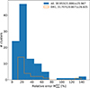 |
Fig. A.1. Relative error of individual dynamical mass estimates for the clusters in the CHEX-MATE sample (blue) and the 24 clusters in the DR1 subsample (orange). We provide the mean (median) and standard deviation for each distribution. |
Appendix B: Intrinsic scatter modelling
The intrinsic scatter of the thermal pressure distribution in clusters is expected to decrease from the core out to ∼0.5 − 1 × R500, where the gravity dominates the structure formation, and then increase towards the outskirts. In Fig. B.1, black markers in the left panel indicate the intrinsic scatter profiles obtained from the joint fit of the UPP and the scatter in Sayers et al. (2023) and Ghirardini et al. (2019). We show in red and green their mean and median.
Following the functional form in Eq. 6 in Ghirardini et al. (2019), we can describe the scatter as a function of σ1, σ0, and x0:
 (B.1)
(B.1)
The dashed line in the central panel in Fig. B.1 gives the best-fitting intrinsic scatter profile model describing the median of the data points from the literature with Eq. (B.1). We observe that the symmetry of this log-parabola shape may force an overestimation (underestimation) of the scatter in the core (outskirts).
As an alternative, we suggest to parametrise the intrinsic scatter profile following Eq. (6), which has the same number of free parameters as Eq. (B.1). The solid line in the central panel in Fig. B.1 shows that Eq. (6) enables a better description of the scatter.
In the right panel in Fig. B.1 we compare the scatter profiles obtained in Sayers et al. (2023) and Ghirardini et al. (2019) to the intrinsic scatter we measure in Sect. 5.1. The filled area corresponds to the intrinsic scatter profile estimated from the joint fit of Planck and XMM-Newton pressure bins with δ as a free parameter. The hatched profile is obtained from the fit of XMM-Newton pressure bins only. Extrapolated regions are shaded.
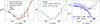 |
Fig. B.1. Intrinsic scatter profiles of the thermal pressure distribution in galaxy clusters as a function of normalised radius. Left: Scatter measured in Sayers et al. (2023) and Ghirardini et al. (2019) indicated with black markers. The red and green profiles give the mean and median in bins, respectively, with the error bars indicating the standard deviation and the median absolute deviation. Centre: Best-fitting scatter models of the median bins following Eq. (6) (solid) and Eq. (B.1) (dashed). Right: Scatter measured in Sayers et al. (2023) and Ghirardini et al. (2019) shown with black markers as in the left panel. The blue shaded areas indicate the 16th to 84th percentiles of the intrinsic scatter profile fitted following Eq. (6) in the joint fit to our data in Sect. 5.1. We show the result from the fit to Planck and XMM-Newton data as in Fig. 4, and the hatched area corresponds to the XMM-Newton-only fit. Extrapolated regions for each case are shaded. |
Appendix C: Validation on simulated profiles
The model presented in Sect. 3 contains a large number of free parameters (global parameters, plus one mass parameter per cluster) and many of them are correlated to each other. For this reason, it seems necessary to validate the method with end-to-end tests. In this section, we present the construction of simulated mock pressure profiles and the fit of the model to these mocks. We first investigate the ability to recover the input parameters under the impact of different intrinsic scatter levels. Then, we perform the fits by considering the individual cluster masses as free parameters.
C.1. Construction of simulated profiles
Following the model in Sect. 3, we build 28 pressure profiles corresponding to the DR1 sample by assuming the MMF3 mass for each cluster. We consider δ = 2/3 + 0.12 and ηT = 1, as well as the gNFW parameters from Arnaud et al. (2010): [P0, c500, α, β, γ]=[8.403, 1.177, 1.0510, 5.4905, 0.3081]. The 28 profiles are drawn from random realisations assuming a given constant intrinsic scatter (not radial dependent), and considering the radial bins corresponding to each data profile (Fig. 1).
Each simulated profile is associated to the covariance matrix of its corresponding data pressure profile (Σdata), including both the XMM-Newton and Planck parts. By doing this, the fits of simulated profiles in Appendix C.2 and C.3 are affected by the same noise level as the data profiles fits in Sect. 5. This is crucial to quantify, for instance, the sensitivity to disentangle the various parameters.
C.2. Sensitivity to intrinsic scatter
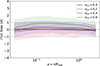 |
Fig. C.1. Bias of the UPP fitted to mock profiles with intrinsic scatter. Colours indicate the results for the different input intrinsic scatter values. We only show cases with values of 0.0, 0.2, 0.4, and 0.6. The solid lines show the mean bias for the 60 realisations, and the shaded areas cover the 16th to 84th percentiles. The grey dashed lines correspond to ±1σ. |
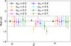 |
Fig. C.2. Bias of ηT, σint, and δ parameters. Colours indicate the different constant intrinsic scatter levels assumed to create the mock profiles. For each case the mean (median) bias as well as the 16th to 84th percentiles are calculated from 60 realisations. |
By taking all M500, i masses fixed to the values used to simulate the profiles, in this section we fit all the global parameters, but Lint, to profiles generated with different intrinsic scatter levels as input. We test the fitting procedure for 8 constant input scatter values that span a realistic range according to previous studies based on observations (Ghirardini et al. 2019; Sayers et al. 2023): σint in [0.0, 0.7]. For each of the input scatter values, we repeat the simulated profiles generation and fitting procedure 60 times to enforce reproducibility. In the fits, we consider uniform priors on the parameters as listed in Table 1. We fit a constant intrinsic scatter (σint(x) = σint) and take the following flat priors: σint ∼ 𝒰(0, 10) and δ ∼ 𝒰(0, 10).
Colour lines in Fig. C.1 show the bias of the best-fit ℙ(x) with respect to the input universal profile when modelling the intrinsic scatter as constant. In particular, they indicate the difference between the best-fit and input ℙ(x) in units of the dispersion of the posterior profiles obtained from the fitting procedure. Solid lines and shaded areas represent the mean and 16th to 84th percentiles for 60 realisations, respectively. For the sake of clarity, we do not show the σint = 0.1, 0.3, 0.5, and 0.7 cases.
In Fig. C.2, we present the bias of the best-fit values for the ηT, σint, and δ parameters in units of the dispersion of the marginalised posterior distributions obtained from the fitting procedure. We give the mean (median) bias for the 60 realisations with crosses (circles) and error bars indicate the 16th to 84th percentiles.
We verify (as can be seen in Fig. C.1) that we obtain unbiased gNFW profiles if σint ≤ 0.6 across the full radial range. When the intrinsic scatter is large, the underlying UPP model is more difficult to recover and up-scattered UPPs are preferred (Fig. C.1). Given the correlation of the gNFW parameters with σint, the scatter parameter tends towards lower values (Fig. C.2, and see also Fig. 4 from the fit to data). For intrinsic scatter values that are lower than our average statistical uncertainties (σint ≲ 0.3, see Fig. 4), it is difficult to distinguish the intrinsic scatter itself from the noise, and the first tends to be underestimated (Fig. C.2), although within 1σ. Regarding δ and ηT, they are unbiasedly recovered for all the tested intrinsic scatter levels (see Fig. C.2). Here, we have only validated the sensitivity to recover models with constant intrinsic scatter profiles. When letting the Lint parameter free, we test in a single realisation of simulations that the fitted value is compatible with zero. We also model the intrinsic scatter following Eq. (6) and obtain an intrinsic scatter profile that decreases with radius (following the tendency observed on data in Sect. 5.1) deviating from a constant scatter at a 2σ level.
C.3. M500 as free parameters
As done for the data analysis in Sect. 5.1, in this section, we consider all the individual cluster M500, i masses as free parameters. The correlation between the global parameters ({P0, c500, α, β, γ; δ; ηT; σint}) and the individual M500, i makes the joint fit very complex. Thus, we take Gaussian priors for M500, i (Table 1, with the MMF3 mass estimates used to build the mock profiles), assuming the uncertainties on the masses to be of ∼25% of the mass values. These uncertainties mimic the typical size of errors associated to dynamical masses (see Sect. 2.2 and Fig. A.1).
We perform the fits on mock profiles simulated with σint = 0.4, a reasonable average intrinsic scatter according to observations (see Fig. 8 in Sayers et al. 2023). Bias on fits are again quantified as the difference between the best-fit and the input in units of the dispersion σ of the posteriors obtained from the fitting procedure: bias = (best-fit − input)/σ. We test different cases, repeating always the profile creation and fitting procedure 60 times:
-
Case A: Priors centred on ’true’ M500, i. We first consider the case in which the Gaussian priors on M500, i are centred on the mass values used to generate the mock pressure profiles. By fixing the power to δ = 2/3 + 0.12, the free parameters are θ = {M500, 1, ..., M500, n; P0, c500, α, β, γ; ηT; σint}. The black line in the top panel in Fig. C.3 shows the bias of the fitted UPP with respect to the truth. We observe that the joint fit gives unbiased pressure profiles. On average, fitted masses are completely compatible with input values (bias of 0.02 ± 0.89). Individual biases of the fitted cluster masses are shown in the bottom panel in Fig. C.3.
-
Case B: Free δ and priors centred on ’true’ M500, i. Similarly, we try fitting the P500 − M500 scaling relation together with the rest of the parameters. Since δ is correlated to P0 and the individual cluster masses, we consider a Gaussian prior for δ. Given the values obtained in the literature (Sect. 3), we take a prior for δ centred on the input value with a scatter of 0.2, that is, 𝒩(2/3 + 0.12, 0.22). We present the bias on the resulting gNFW profile in red in Fig. C.3, where we observe that the fitted UPP is unbiased. Compared to Fig. C.1, here the bias in units of σ is closer to zero because uncertainties derived from posterior distributions are larger, but in both cases the relative bias is of the order of 2.5%. In this case, individual masses are also unbiasedly recovered (average bias of 0.04 ± 0.81) and the best-fitting δ are at −0.47 ± 0.89 with respect to the input. Even if within 1σ, this bias on δ might mean that the mass range covered by the clusters in the sample is not large enough to fully leverage the mass dependence to distinguish between δ and the rest of free parameters.
-
Case C: Scattered priors on M500, i. When using real data, the mass estimates might be scattered with respect to the true mass of each cluster. In order to simulate this, we repeat the fit but taking mass priors centred on masses scattered by ∼20% with respect to the ’true’ M500, i. We consider here fixed δ = 2/3 + 0.12. The blue profile in Fig. C.3 indicates that even in this case we are able to recover unbiased pressure profiles. Similarly, fitted masses are compatible with ’true’ M500, i, the average bias for the masses being of −0.05 ± 0.98.
-
Case D: Biased priors on M500, i. Finally, we simulate the case in which the priors on the masses are systematically biased with respect to the ’true’ M500, i, that is, the centre of the Gaussian mass priors are shifted with respect to the true masses. By biasing the mass priors low by ∼20%, we recover overestimated pressure profiles (green profile in Fig. C.3) and underestimated masses (biased by −2.72 ± 0.84). This case shows the impact of mass priors, affecting also the shape of the best-fit gNFW.
All four cases give unbiased ηT reconstructions (−0.11 ± 1.02, 0.12 ± 1.18, 0.10 ± 1.09, and −0.19 ± 0.82 respectively for A, B, C, and D) and, as in Appendix C.2, σint is systematically underestimated but the average bias is less than the typical measurement uncertainty (−0.60 ± 0.94, −0.32 ± 0.87, −0.41 ± 0.90, and −0.67 ± 0.83 for A, B, C, and D, respectively).
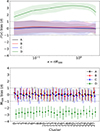 |
Fig. C.3. Top: Bias of the UPP fitted to mock profiles with an intrinsic scatter of σint = 0.4. The colours indicate the results with different priors for M500, i and δ, from case A to D, as detailed in the text. The solid lines show the mean bias for the 60 realisations, and the shaded areas cover the 16th to 84th percentiles. Bottom: Bias of the fitted individual cluster masses. For each cluster, we give the median bias and dispersion from the 60 realisations. The dashed lines indicate ±1σ. |
Finally, by fixing the UPP parameters to values different to the ones used to create the mock profiles, we have verified, as expected, that we recover biased cluster masses (average ∼ − 4.5σ and ∼1σ biases for [P0, c500, α, β, γ]=[6.72, 1.18, 1.08, 4.30, 0.31] and [P0, c500, α, β, γ]=[3.36, 1.18, 1.08, 4.30, 0.31], respectively). The impact of the assumed gNFW profile on the fitted masses for data pressure profile fits is quantified in Sect. 5.2. We have also verified that we recover a Lint compatible with zero if this is a free parameter in the fit, also in the case in which we fit an intrinsic scatter modelled following Eq. (6). In this case, from the fit of one realisation of simulations we recover an intrinsic scatter profile compatible with a constant at 1σ level.
C.4. Summary
In conclusion, unless the intrinsic scatter of the profiles is larger than σint = 0.6, for fixed M500, i we are able to reconstruct unbiased ℙ(x),δ, and ηT. It is the reconstruction of the intrinsic scatter itself that is intricate and will depend on its actual value. It goes without saying that these conclusions also depend on the uncertainties associated to the pressure profile data we are fitting and will change with data quality (Sect. 5).
When letting individual cluster masses vary in the fit, we observe that, as expected, the outcomes are biased if mass priors are biased. On the contrary, if our mass estimates are scattered with respect to the true masses, we are able to recover the ’true’ M500, i and unbiased pressure profiles. The free parameters in the model are strongly correlated and the likelihood becomes flat when close to the best-fit values in the multi-variable space. As a consequence, the prior distributions we consider for the mass parameters will determine the scale of the fitted masses. Regarding the P500 − M500 scaling relation, it can be difficult to disentangle the power law δ from the rest of the free parameters in the model, the gNFW amplitude P0 and individual cluster masses being also entangled in the pressure profile amplitude (see Fig. D.1 from the application of the method to data).
Appendix D: Posterior distributions of parameters fitted to data
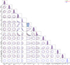 |
Fig. D.1. Posterior probability distributions (1D and 2D) of the free parameters fitted to XMM-Newton and Planck pressure profiles. We only show the masses for three of the 24 fitted clusters, illustrating the strong correlations between the individual mass parameters. Green, red, and blue correspond respectively to δ = 2/3, 2/3 + 0.12, and δ free cases. Cluster masses are given in 1014 M⊙ units. |
We present in Fig. D.1 the 1D and 2D posterior distributions for the parameters fitted to data pressure profiles in Sect. 5.1. For visualisation purposes, we only show the posterior probability distributions of three cluster mass parameters as an example to illustrate their degeneracies. Different colours correspond to results for different values of δ.
In Fig. D.2, we compare the marginalised posterior distributions of the individual M500, i parameters to the prior distributions assumed for each of them.
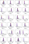 |
Fig. D.2. Marginalised posterior distributions of the 24 cluster masses obtained from the joint fits of UPP and M500, i parameters to data pressure profiles. We follow the same colour scheme as in Fig. D.1. In grey, we indicate the prior distribution considered for each parameter, corresponding to Gaussian distributions centred on the dynamical mass estimates from Sereno et al. (2025) with dynamical mass measurement errors as their standard deviations. All masses are in 1014 M⊙ units. |
Appendix E: UPP parameters from the literature
Table E.1 summarises the gNFW and δ parameters from the literature considered in Sect. 5.2. These gNFW profiles are shown in Fig. E.1, distinguishing between the models reconstructed assuming δ = 2/3 and δ = 2/3 + 0.12.
Parameters from the literature for UPP.
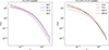 |
Fig. E.1. UPPs from the literature. The parameters of the gNFW model for each case are summarised in Table E.1. We distinguish between the models reconstructed assuming δ = 2/3 (left) and δ = 2/3 + 0.12 (right). |
All Tables
Best-fit parameters from the joint fit of pressure profiles assuming dynamical mass priors and for different δ values.
All Figures
|
Fig. 1. Pressure profiles for the 28 galaxy clusters investigated in this work reconstructed from XMM-Newton (orange) and Planck (blue) data. XMM-Newton data profiles below r/R500 = 0.03 are shaded. These pressure bins are not considered in our analysis (see text). |
| In the text | |
|
Fig. 2. Normalised data pressure profiles, best-fit gNFW models, and their relative difference. Top: Coloured profiles show the individual data pressure profiles (from Fig. 1) for the 24 clusters normalised by the best P500, i and R500, i values when fitting the individual masses with dynamical mass estimates as priors. Green, red, and blue correspond to the fits assuming respectively δ = 2/3, δ = 2/3 + 0.12, and δ as a free parameter. Bottom: Data pressure profiles in grey, normalised by P500, i and R500, i values, with masses fixed in the fit and set to the dynamical mass estimates. The solid black profile in each panel indicates the best-fit gNFW profile for that case, with the dotted profiles showing the fitted intrinsic scatter ℙ(x)exp[±σint(x)]. The dashed profiles in the top (bottom) panels correspond to the best-fit gNFW for the mass-fixed (fitted) cases. |
| In the text | |
|
Fig. 3. Masses obtained from the joint fit to data by taking Gaussian priors centred on dynamical estimates. We compare the results to the dynamical (top) and MMF3 (bottom) mass estimates. The colour scheme is identical to that in Fig. 2 for the different values of δ. Uncertainties of fitted masses are calculated as the standard deviation of the marginalised posterior distribution for each cluster mass parameter. |
| In the text | |
|
Fig. 4. Scatter of pressure profiles for the 24 clusters in our sample. The shaded area indicates the 16th to 84th percentiles for the intrinsic scatter profile fitted to data pressure profiles (δ free case). The intrinsic scatter may not be reliably constrained beyond x ∼ 0.4. The dashed line indicates the scatter of the individual normalised profiles with respect to the best-fit gNFW model. Statistical uncertainties of the individual pressure profiles are indicated with crosses and circles for the pressure bins corresponding to XMM-Newton and Planck data, respectively. All scatters are given in P500ℙ(x) units. |
| In the text | |
|
Fig. 5. Distribution of the 24 best-fit M500 obtained from the thermal pressure profile fits with ηT free. We present the average mass of the sample for fixed UPPs from the literature, shown with circles and diamonds for the cases where ηT is free in the fit and fixed to ηT = 1.05, respectively. We also show the |
| In the text | |
|
Fig. A.1. Relative error of individual dynamical mass estimates for the clusters in the CHEX-MATE sample (blue) and the 24 clusters in the DR1 subsample (orange). We provide the mean (median) and standard deviation for each distribution. |
| In the text | |
|
Fig. B.1. Intrinsic scatter profiles of the thermal pressure distribution in galaxy clusters as a function of normalised radius. Left: Scatter measured in Sayers et al. (2023) and Ghirardini et al. (2019) indicated with black markers. The red and green profiles give the mean and median in bins, respectively, with the error bars indicating the standard deviation and the median absolute deviation. Centre: Best-fitting scatter models of the median bins following Eq. (6) (solid) and Eq. (B.1) (dashed). Right: Scatter measured in Sayers et al. (2023) and Ghirardini et al. (2019) shown with black markers as in the left panel. The blue shaded areas indicate the 16th to 84th percentiles of the intrinsic scatter profile fitted following Eq. (6) in the joint fit to our data in Sect. 5.1. We show the result from the fit to Planck and XMM-Newton data as in Fig. 4, and the hatched area corresponds to the XMM-Newton-only fit. Extrapolated regions for each case are shaded. |
| In the text | |
|
Fig. C.1. Bias of the UPP fitted to mock profiles with intrinsic scatter. Colours indicate the results for the different input intrinsic scatter values. We only show cases with values of 0.0, 0.2, 0.4, and 0.6. The solid lines show the mean bias for the 60 realisations, and the shaded areas cover the 16th to 84th percentiles. The grey dashed lines correspond to ±1σ. |
| In the text | |
|
Fig. C.2. Bias of ηT, σint, and δ parameters. Colours indicate the different constant intrinsic scatter levels assumed to create the mock profiles. For each case the mean (median) bias as well as the 16th to 84th percentiles are calculated from 60 realisations. |
| In the text | |
|
Fig. C.3. Top: Bias of the UPP fitted to mock profiles with an intrinsic scatter of σint = 0.4. The colours indicate the results with different priors for M500, i and δ, from case A to D, as detailed in the text. The solid lines show the mean bias for the 60 realisations, and the shaded areas cover the 16th to 84th percentiles. Bottom: Bias of the fitted individual cluster masses. For each cluster, we give the median bias and dispersion from the 60 realisations. The dashed lines indicate ±1σ. |
| In the text | |
|
Fig. D.1. Posterior probability distributions (1D and 2D) of the free parameters fitted to XMM-Newton and Planck pressure profiles. We only show the masses for three of the 24 fitted clusters, illustrating the strong correlations between the individual mass parameters. Green, red, and blue correspond respectively to δ = 2/3, 2/3 + 0.12, and δ free cases. Cluster masses are given in 1014 M⊙ units. |
| In the text | |
|
Fig. D.2. Marginalised posterior distributions of the 24 cluster masses obtained from the joint fits of UPP and M500, i parameters to data pressure profiles. We follow the same colour scheme as in Fig. D.1. In grey, we indicate the prior distribution considered for each parameter, corresponding to Gaussian distributions centred on the dynamical mass estimates from Sereno et al. (2025) with dynamical mass measurement errors as their standard deviations. All masses are in 1014 M⊙ units. |
| In the text | |
|
Fig. E.1. UPPs from the literature. The parameters of the gNFW model for each case are summarised in Table E.1. We distinguish between the models reconstructed assuming δ = 2/3 (left) and δ = 2/3 + 0.12 (right). |
| In the text | |
Current usage metrics show cumulative count of Article Views (full-text article views including HTML views, PDF and ePub downloads, according to the available data) and Abstracts Views on Vision4Press platform.
Data correspond to usage on the plateform after 2015. The current usage metrics is available 48-96 hours after online publication and is updated daily on week days.
Initial download of the metrics may take a while.