| Issue |
A&A
Volume 704, December 2025
|
|
|---|---|---|
| Article Number | A198 | |
| Number of page(s) | 19 | |
| Section | Stellar structure and evolution | |
| DOI | https://doi.org/10.1051/0004-6361/202556699 | |
| Published online | 09 December 2025 | |
Tracking optical variability and outflows across the accretion states of the black hole transient MAXI J1820+070
1
INAF, Osservatorio Astronomico di Brera, Via E. Bianchi 46, I-23807 Merate (LC), Italy
2
Center for Astrophysics and Space Science (CASS), New York University Abu Dhabi, PO Box 129188 Abu Dhabi, UAE
3
INAF–Osservatorio di Astrofisica e Scienza dello Spazio, Via Piero Gobetti 101, I-40129 Bologna, Italy
4
Universidad Andrés Bello, Av. Fernández Concha 700, Las Condes, Santiago, Chile
5
Dipartimento di Fisica, Università degli Studi di Milano, Via Celoria 16, I-20133 Milan, Italy
6
Instituto de Astrofísica de Canarias (IAC), Vía Láctea s/n, La Laguna, E-38205 S/C de Tenerife, Spain
7
Departamento de Astrofísica, Universidad de La Laguna, La Laguna, E-38205 S/C de Tenerife, Spain
8
INAF Istituto di Astrofisica e Planetologia Spaziali, Via del Fosso del Cavaliere 100, I-00133 Rome, Italy
9
Al Sadeem Observatory, Al Wathba South, Abu Dhabi, UAE
10
Rizal Technological University, Mandaluyong City, Philippines
11
Instituto Nacional de Astrofísica, Óptica y Electrónica (INAOE), Luis Enrique Erro #1, Tonantzintla, Puebla C.P. 72840, Mexico
★ Corresponding author: This email address is being protected from spambots. You need JavaScript enabled to view it.
Received:
1
August
2025
Accepted:
16
October
2025
Abstract
We present a study of the evolution of the minute-timescale optical variability and of the optical spectroscopic signatures of outflows in the black hole X-ray binary MAXI J1820+070 during its main 2018 outburst and subsequent re-brightenings. Multi-filter, minute-cadence optical light curves were obtained with the Las Cumbres Observatory network and the Al Sadeem Observatory (UAE) over 2018–2020, complemented by archival X-ray data from Swift/BAT, Swift/XRT, and MAXI. We also acquired contemporaneous low-resolution optical spectra with the 2.1 m OAN San Pedro Mártir (Mexico), the 2.1 m OAGH Cananea (Mexico), and the G.D. Cassini 1.5 m telescope in Loiano (Italy). The optical fractional root mean square is highest in the hard state and is best described by short-timescale flickering that is stronger at longer wavelengths. This suggests that the minute-timescale optical variability is driven by the jet in the hard state. In this scenario, the variability could be due to variations in the inflow that inject velocity fluctuations at the base of the jet (internal shock model). The variability is then quenched in the soft state, with any residual signal likely associated with variability in the accretion flow. This is in agreement with the accretion-ejection coupling in black hole binaries and confirms that the variability signature of the jet is present at optical wavelengths in all hard states. In the dimmest hard states, any residual optical variability may instead be linked to cyclo-synchrotron emission from the hot flow. The optical spectra reveal double-peaked emission lines and possible signatures of cold winds during the hard state. Such winds were previously reported in this source during the main 2018 outburst; here we provide one of the first tentative detections of their presence during the subsequent re-brightenings. The absence of optical wind signatures in the soft state likely reflects a higher level of disc ionisation driven by the increased X-ray flux, which suppresses the low ionisation features detectable in the optical band.
Key words: stars: black holes / stars: jets / stars: winds / outflows
© The Authors 2025
 Open Access article, published by EDP Sciences, under the terms of the Creative Commons Attribution License (https://creativecommons.org/licenses/by/4.0), which permits unrestricted use, distribution, and reproduction in any medium, provided the original work is properly cited.
This article is published in open access under the Subscribe to Open model. This email address is being protected from spambots. You need JavaScript enabled to view it. to support open access publication.
1. Introduction
Black hole (BH) low-mass X-ray binaries (LMXBs) are compact systems hosting a stellar-mass BH and a main-sequence star with a typical mass of ≤1 M⊙. BHs in these systems undergo a process of accretion of matter and angular momentum from the companion star through Roche lobe overflow, which leads to the formation of an accretion disc around the compact object. BH LMXBs typically have a transient nature, alternating between long quiescent states (months to years), with a low level of activity and X-ray luminosities (1031 − 33 erg s−1), and states of enhanced activity called outbursts, triggered by hydrogen ionisation, which typically occur on shorter timescales (weeks to months) and display X-ray luminosities (LX) of 1036 − 38 erg s−1.
At the beginning of an outburst, the LX of the source reaches ≥1038 erg s−1 very rapidly. For most of this luminosity range, the X-ray state is observed to be ‘hard’, characterised by high X-ray variability (up to 40% fractional root mean square in the case of GX 339-4; Motta et al. 2015; see also Muñoz-Darias et al. 2011) and by an X-ray spectrum peaking at ∼100 keV, possibly originating in thermal Comptonisation in a hot plasma (the corona) around the accretion disc. After a while, the system transitions to the ‘soft’ state, and the X-ray spectrum is dominated by a black-body component that peaks at ∼1 keV, probably originating in the accretion disc. In the soft state, variability drops significantly. The system then typically fades slowly and transitions back to the hard state before going back to quiescence (see Belloni et al. 2016 for a review).
Variability is also expected at lower energies, though the picture is rather complex. The optical emission during outbursts is dominated by the accretion disc. In particular, two primary components contribute significantly: (i) the viscously heated disc, which varies more slowly, on timescales of days to weeks, driven by changes in the mass accretion rate from the companion star and by the structural evolution in the disc itself (e.g. variations in the temperature profile or the presence of heating or cooling fronts), and (ii) X-ray reprocessing, where variable X-ray emission from the inner disc irradiates the outer disc and/or the companion star surface, producing optical and infrared (OIR) emission that can follow the X-ray light curve with a characteristic smearing due to the finite light travel time and reprocessing efficiency (see e.g. echo-mapping studies such as O’Brien et al. 2002 and van Paradijs & McClintock 1994).
In addition to these dominant sources, other forms of variability contribute on intermediate timescales (hours to days). These include super-humps produced by precessing or warped accretion discs (e.g. Thomas et al. 2022) and ellipsoidal modulations of the companion star, though the latter are typically only visible in quiescence. Furthermore, rapid variability on timescales from minutes down to sub-seconds has been observed in some systems, particularly in the redder bands. This has been interpreted as arising from several possible components: a hot, magnetised, geometrically thick and optically thin inner flow emitting synchrotron radiation (Veledina et al. 2013), wind-related variability (e.g. changes in the blue component of P-Cygni absorption lines; Vincentelli & Muñoz-Darias 2025), or the jet, which is discussed in more detail in the following section. The combination and relative contributions of these components can lead to diverse OIR variability patterns across a broad range of timescales.
Several studies of BH LMXBs have shown that part of the optical emission can originate in synchrotron emission from relativistic compact jets (e.g. Corbel & Fender 2002; Chaty et al. 2003; Buxton & Bailyn 2004; Homan et al. 2005; Russell et al. 2010, 2011; Baglio et al. 2018b; Saikia et al. 2019). Jets are launched from the central regions of BH LMXBs and typically produce a flat (optically thick) radio spectrum that transitions to optically thin at OIR frequencies, resulting in a negative power law (Corbel & Fender 2002; Gandhi et al. 2011; Russell et al. 2013a). Interestingly, a strong coupling between accretion and ejection has been observed in several BH LMXBs: the emission of compact jets when the outburst is in the hard state and is then replaced by optically thin discrete ejecta during the hard-to-soft transitions (visualised as powerful radio flares and resolved, superluminal ejecta seen in radio images). The jet is finally completely quenched at all wavelengths during soft states (for a review, see Fender & Gallo 2014). In these states, hot winds are often detected through X-ray spectroscopy as blueshifted absorption lines produced by highly ionised material (Ponti et al. 2012; Díaz Trigo & Boirin 2016; Neilsen & Degenaar 2023). In addition, recent findings show signatures of the emission of cold winds through optical spectroscopy, particularly with the observation of P-Cyg line profiles in He and H lines in the spectra of some BH LMXBs (V404 Cyg, V4641 Sgr, MAXI J1820+070, and up to ten other sources; Muñoz-Darias et al. 2016, 2018, 2019; Sánchez-Sierras & Muñoz-Darias 2020; Panizo-Espinar et al. 2022). These cold winds have also been observed during hard states, in some cases simultaneously with radio jets, indicating that the two phenomena can coexist depending on the accretion flow configuration.
Jet emission has been found to be strongly variable on short (from sub-second to minute) timescales. Several coordinated X-ray/OIR observations have also shown correlated short-timescale variability with lags of the order of fractions of seconds, with the OIR emission lagging the X-rays (∼0.1 s for several BH LMXBs; Gandhi et al. 2008; Casella et al. 2010; Gandhi et al. 2017; Paice et al. 2019). This lagged, correlated short-timescale variability has been explained, for example, by the internal shock model (Malzac 2013, 2014; Malzac et al. 2018), which connects the variations in the accretion flow, observed at X-ray frequencies, to the injection of velocity fluctuations at the jet base. These fluctuations drive internal shocks at large distances from the BH, giving rise to variable synchrotron emission, therefore affecting the overall radio–OIR emission. This model has been successful so far in reproducing the observations of GX 339-4 (Drappeau et al. 2017; Malzac et al. 2018; Vincentelli et al. 2019) and the neutron star X-ray binary 4U 0614+091 (Marino et al. 2020), and has also been suggested to explain the high fractional root mean square (rms) observed in the OIR for the BH LMXBs MAXI J1535−571 (Baglio et al. 2018b; Vincentelli et al. 2021), MAXI J1836−194 (Péault et al. 2019), and MAXI J1820+070 (Tetarenko et al. 2021).
2. MAXI J1820+070
The optical transient ASASSN-18ey was first detected on March 6, 2018, by the All-Sky Automated Survey for Supernovae (ASAS-SN) survey (V = 14.9; Denisenko 2018). A few days later, on March 11, the source was independently identified in X-rays by the Monitor of All-sky X-ray Image Gas Slit Camera (MAXI/GSC) nova alert system, which reported it as a bright, uncatalogued X-ray source and designated it MAXI J1820+070 (Kawamuro et al. 2018). Follow-up on March 13 with the Las Cumbres Observatory (LCO) network 1 m telescopes revealed a brightened optical counterpart, several magnitudes above its Panoramic Survey Telescope & Rapid Response System (Pan-STARRS) quiescent level. The strong X-ray emission and its location on the optical/X-ray luminosity plane indicated a LMXB with a likely BH primary (Baglio et al. 2018c), later confirmed by dynamical measurements showing a mass ratio of q ∼ 0.04 and a compact object mass exceeding the neutron star limit (Torres et al. 2019, 2020). Very long-baseline interferometry parallax placed the source at 2.96 ± 0.33 kpc, constraining its luminosity and jet energetics (Atri et al. 2020).
Short-timescale optical variability was observed, including > 100% amplitude flares on ∼100 ms and ∼10 ms scales (Sako et al. 2018). Sub-second variability, strongest in red, was detected with the ULTRA-fast CAMera (ULTRACAM) on the New Technology Telescope (NTT), suggesting a jet origin (Gandhi et al. 2018). A flat radio spectrum observed on March 18 with the Radio Astronomy Telescope of the Academy of Sciences (RATAN-600) supported this interpretation (Trushkin et al. 2018), and later studies linked the fast optical variability to synchrotron emission from the jet (Paice et al. 2019; Tetarenko et al. 2021; Thomas et al. 2022). In the near-infrared (NIR), Ks ∼ 10.2 with ∼25% rms variability was detected on March 19 using the Very Large Telescope High Acuity Wide-field K-band Imager (VLT/HAWK-I; Casella et al. 2018). On April 8–9, a bright mid-infrared (MIR) counterpart (∼0.3 Jy) was found, making MAXI J1820+070 the brightest MIR transient LMXB observed (Russell et al. 2018; Echiburú-Trujillo et al. 2024).
Following an initial rise and hard-state plateau, the Neutron star Interior Composition Explorer (NICER) instrument observed a flux decline in mid-May 2018, followed by an increase with spectral softening, indicating a transition to the hard-intermediate state by early July and then to the soft state (Homan et al. 2018). The Arcminute Microkelvin Imager Large Array (AMI-LA) detected quenched radio emission and flaring, consistent with this transition (Bright et al. 2018b). The evolution has been detailed through multi-wavelength studies (Bright et al. 2020; Homan et al. 2020) and X-ray reverberation lag studies (Kara et al. 2019). Broadband X-ray data from the Insight-Hard X-ray Modulation Telescope (HXMT) instrument revealed an extended, jet-like corona in the hard state (You et al. 2021), though recent X-ray polarisation results on different systems (e.g. Swift J1727) suggest that the corona is generally unlikely to be extended in this way in the hard state. Espinasse et al. (2020) reported X-ray sources aligned with the radio jets, best interpreted as discrete ejecta interacting with the ISM on large scales, rather than with the corona or the hard state compact jets.
A sharp rise in hard X-ray flux after September 22, 2018 (MJD 58383), detected by MAXI/GSC, signaled a soft-to-hard transition (Negoro et al. 2018). Radio detection by AMI-LA on September 24 confirmed the reactivation of the jet (Bright et al. 2018a), with optical signs of jet activity (increased flux and redder colour) observed by LCO on October 12 (Baglio et al. 2018a; Echiburú-Trujillo et al. 2024; Özbey Arabacı et al. 2022). After nearing quiescence (Russell et al. 2019a), the source showed an unexpected optical re-brightening (Ulowetz et al. 2019; Baglio et al. 2019).
The re-brightening was also seen in X-rays (Swift/XRT, March 10, 2019; Bahramian et al. 2019) and radio (AMI-LA; Williams et al. 2019). Flux declined through April–May, with dimming in both X-rays and the optical (Tomsick & Homan 2019; Zampieri et al. 2019). A second brightening followed in August 2019, first in the optical (Hambsch et al. 2019), then in X-rays and radio (Xu et al. 2019; Bright et al. 2019), peaking in 10 days and lasting 70 days. A third re-brightening occurred in February 2020 in both the optical and X-rays (Adachi et al. 2020; Sasaki et al. 2020). By June 29, 2020, the source reached g′ = 18.79 ± 0.01, still 0.6 mag above its Pan-STARRS quiescent level. Another optical brightening was seen in March 2021 by the LCO X-ray Binary New Early Warning System (XB-NEWS; Baglio et al. 2021b), with flux declining by late April but remaining above quiescence (Baglio et al. 2021a). Low-level activity continued until June 2023, when the source finally returned to full optical quiescence (Baglio et al. 2023).
3. Short-timescale variability: Observations and data analysis
In this paper we report on an optical campaign performed on MAXI J1820+070. The system was regularly monitored since its first activity with the LCO network of robotic 1-m and 2-m telescopes, using the optical filters Y, i′,r′, R, V, and g′. In addition to these, many observations have been collected with the Meade LX850 16-inch (41-cm) telescope of the Al Sadeem Observatory (UAE), as part of the monitoring that started in 2018, using the ‘blue’, ‘green’, and ‘red’ Baader LRGB (Luminance, Red, Green, and Blue) CCD-Filters (which approximately correspond to the central wavelengths of the g′, V, and R filters, respectively; see Russell et al. 2018 and Russell et al. 2019b for details). Although the full optical light curves are shown in the upper panel of Fig. 1 (until MJD 59000; May 31, 2020), in this work we specifically focused on short-timescale (minutes) observations of the target, which happened sporadically in the period of observations with the i′ and g′ filters with LCO (Table A.1) and with all the Al Sadeem Observatory filters (Table B.1). We also retrieved public X-ray observations taken with Swift/BAT (Burst Alert Telescope), Swift/XRT (X-Ray Telescope), and MAXI in order to have simultaneous X-ray observations concurrent with the optical monitoring.
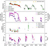 |
Fig. 1. First panel: optical LCO (g′ and i′) and Al Sadeem (g′, V, and R) light curves of MAXI J1820+070 during its 2018-2019 outburst. Magnitudes are not corrected for reddening. Second panel: Swift/BAT (purple), Swift/XRT (pink), and MAXI/GSC (dark purple) count rates vs MJD. Swift/BAT counts have been divided by 100 for visualisation purposes. Third panel: MJD vs. fractional rms variability amplitude evaluated for the time-resolved optical light curves obtained with the LCO and Al Sadeem observations. Fourth panel: MJD vs. hardness ratio evaluated as BAT/MAXI count rates (HRBAT/MAXI) and XRT (2–10 keV)/XRT (0.5–2 keV) count rates (HRXRT). The first panel is available at the CDS. |
3.1. Optical photometry with LCO
MAXI J1820+070 was regularly monitored since its discovery with the LCO 1-m and 2-m telescopes, as part of an ongoing monitoring of ∼50 LMXBs, coordinated by the Faulkes Telescope Project1 (Lewis et al. 2008). The exposure time varied depending on the filter, the phase of the outburst, and the aim of the observation. For general outburst monitoring, the exposure time varied between 20 s and 200 s in all filters; for the timing observations instead, the single exposures lasted in general 20–60 s, with filters alternating in most cases. In Table A.1, a complete log of the fast-timing observations is reported for completeness.
Magnitudes were extracted using multi-aperture photometry (MAP; Stetson 1990) performed with the XB-NEWS pipeline (Russell et al. 2019b; Goodwin et al. 2020). For each reduced image, XB-NEWS first detects sources using SExtractor (Bertin & Arnouts 1996) and solves for the astrometric solution using astrometry.net (Lang et al. 2010), matching against Gaia Data Release (DR) 2 positions. If the target is not detected within 1″ of its known coordinates at the default threshold, the pipeline re-runs detection at a lower threshold. If still undetected, forced photometry is performed at the target position. Photometry is carried out for all sources using both MAP and fixed-aperture photometry, with aperture radii scaled to an appropriate multiple of the point spread function (PSF) full width at half maximum (FWHM). Light curves are then constructed using the DBSCAN clustering algorithm (Ester et al. 1996). Calibration of i′- and g′-band magnitudes is performed against an enhanced version of of the Asteroid Terrestrial-impact Last Alert System Reference Catalog (ATLAS-REFCAT2; Tonry et al. 2018), which incorporates Pan-STARRS DR1 (Chambers et al. 2016) and APASS DR10 (American Association of Variable Star Observers Photometric All-Sky Survey; Henden et al. 2018). A photometric model is fit to the light curves (in magnitudes) of matched and unmatched sources, including spatially variable zero points, PSF-based terms, and source-specific mean magnitudes (Bramich & Freudling 2012). The model excludes colour terms due to limited multi-band coverage, introducing only small systematic errors (< (1 − 2)%) in absolute calibration. The model is fitted iteratively with outlier down-weighting to mitigate the effect of intrinsic variability. For Sloan Digital Sky Survey (SDSS) i′ and g′ filters, XB-NEWS uses the Pan-STARRS1 standard iP1 and gP1 magnitudes in the AB system. The final model is applied to calibrate all light curves, including that of the target. If forced photometry was required for the target, measurements with uncertainties > 0.25 mag were discarded as unreliable. For more details about the pipeline concept and implementation, see Russell et al. (2019b) and Goodwin et al. (2020).
The resulting g′ and i′ light curves for the monitoring during the 2018 outburst and the three subsequent reflares (until MJD 59000; May 31, 2020) are shown in the upper panel of Fig. 1. Portions of this dataset are also published in Russell et al. (2019b), Echiburú-Trujillo et al. (2024), Banerjee et al. (2024), Yang et al. (2025), and Bright et al. (2025). For single light curves, see Appendix A.
3.2. Optical photometry with the Al Sadeem Observatory
MAXI J1820+070 was observed with the Meade LX850 16-inch (41 cm) telescope of the Al Sadeem Observatory (UAE)2, using the ‘blue’, ‘green’, and ‘red’ Baader LRGB CCD-Filters (central wavelengths 463, 538, and 638 nm, respectively), which approximately correspond to the central wavelengths of the g′ (475 nm), V (545 nm), and R (641 nm) filters, respectively. Observations were performed during most of the source activity, with exposure times ranging from 30 to 60 s. Photometric measurements on some dates were previously reported in Baglio et al. (2018a, 2019, 2021a), Russell et al. (2018, 2019b), and Echiburú-Trujillo et al. (2024). Similar to the LCO observations, on several dates sequences of observations were acquired in the three filters, in order to measure short-timescale variability. Here we report on observations acquired during the main outburst, between MJD 58200 (March 23, 2018) and 58430 (November 8, 2018), including rms variability measurements for the first time. A complete log of the variability observations is presented in Table B.1.
All images were bias and flat-field corrected using standard procedures and aperture photometry was performed using the daophot tool within MIDAS3. Calibration was performed against a group of seven isolated field stars, with magnitudes calibrated in the APASS catalogue in the g′, V and r′ filters. Since the Al Sadeem ‘red’ filter corresponds to the Bessell R filter and not the SDSS r′ filter, while the APASS catalogue provides magnitudes in r′, we applied the appropriate transformation from r′ to R using the colour equations provided by Jordi et al. (2006). The results of the photometry are shown in Fig. 1, upper panel.
3.3. X-ray campaign
MAXI J1820+070 was monitored with different X-ray satellites since it was first detected by MAXI/GSC on March 11, 2018 (MJD 58188). For this work, we used the public observations from the monitoring of the 2018/2019 outburst by Swift/BAT (15–150 keV)4 and Swift/XRT (0.5–10 keV)5, and by MAXI/GSC (2–10 keV)6. We converted the fluxes from both Swift/BAT and MAXI into Crab units to normalise their instrumental responses and thus derive a hardness ratio between them. For this, we used the following conversion factors: 1 Crab = 0.22 ph/s/cm2 and 1 Crab = 3.45 ph/s/cm2 for Swift/BAT and MAXI, respectively7. Then, we defined the hardness ratio HRBAT/MAXI as the ratio between the flux of Swift/BAT and MAXI in Crab units (Fig. 1, last panel). Similarly, using Swift/XRT data we evaluated the hardness ratio HRXRT, defined as the ratio of the 2−10 keV XRT count rates to the 0.5−2 keV XRT count rates (Fig. 1, last panel).
4. Short-timescale variability: Results
4.1. Optical variability and X-ray hardness analysis
To estimate the amount of short-timescale variability of the optical light curves, we evaluated the fractional rms variability amplitude following Vaughan et al. (2003). In particular, the quantity is defined as follows:
 (1)
(1)
where σerr is the error on the single flux value (this value was then squared and averaged for each sample, and  is the mean magnitude value of the sample. S, instead, is the variance of the sample, and it is defined as
 (2)
(2)
where N is the total number of observations in the sample, and xi is the single flux value of the i-th observation in the sample.
The fractional rms variability amplitude is found to vary from epoch to epoch, in all bands, as can be observed in Fig. 1 (third panel), going from ∼0 to ∼20%. This variability is sampled over timescales corresponding to frequencies approximately between ∼7 × 10⁻⁴ and ∼0.03 Hz, depending on the duration and cadence of the individual light curves.
During the main outburst (March 2018 – February 2019), the fractional rms variability amplitude calculated for both the LCO and Al Sadeem datasets is found to be higher (∼5% and ∼6% on average in the LCO g′ and i′ band, respectively) during the long hard-state plateau happening before ∼MJD 58300 (July 1, 2018), and then gets lower (on average, ∼1% in both bands) after the transition to the soft-intermediate state, until MJD 58383 (September 22, 2018, i.e. the time of the transition to the hard X-ray spectral state; see Fig. 1). After that, the fractional rms variability amplitude increases again, reaching ∼9% in the i′ band. During the first and second re-brightenings, only one i′-band fractional rms variability amplitude measurement is available for each, with values of ∼7% and ∼10%, respectively. An interesting feature is observed on MJD ∼ 58620-30 (i.e. May 17–27, 2019), with the fractional rms variability amplitude in the g′ band suddenly increasing, reaching up to ∼20% on MJD 58627.5. At that time, the source was in an apparent quiet state soon after the end of the first re-brightening, with a magnitude of g′∼16.
The last two panels of Fig. 1 suggest a possible correlation between the fractional rms variability amplitude of the optical curves and the hardness evolution of the X-ray spectrum. Motivated by this, we investigated whether changes in the optical fractional rms could be directly linked to variations in the X-ray hardness. The results are shown in Figs. 2 and B.1 (top panel) for the LCO and Al Sadeem datasets, respectively, using as hardness ratio the quantity HRBAT/MAXI. A clear correlation is observed in the LCO dataset, with the optical rms increasing towards harder spectra across all filters. The Al Sadeem data show greater scatter, likely due to lower data quality, and exhibit only a mild correlation, most noticeable in the R band. The correlation parameters are listed in Table 1.
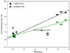 |
Fig. 2. Hardness ratio (calculated as BAT/MAXI) vs fractional rms of the optical LCO g′ (green dots) and i′ (black dots) data. Linear fits to the data are represented with dashed green and black lines, respectively, to show the increasing trend of the fractional rms with the hardness. |
Results of the correlation study using the hardness ratio calculated as the ratio between the BAT (hard) and the MAXI (soft) X-ray fluxes vs. the optical fractional rms of the LCO g′ and i′ and Al Sadeem g′, V, and R light curves.
In all bands, a positive Pearson coefficient indicates a linear correlation between the fractional optical rms variability amplitude and the hardness of the X-ray spectrum. Specifically, Pearson coefficients greater than 0.8 for the LCO g′ and i′ bands suggest a strong or very strong linear correlation between these two quantities.
Similarly, for both the LCO and Al Sadeem datasets we plotted the optical fractional rms variability amplitude against the hardness ratio HRXRT. This correlation analysis employs softer X-ray photons than those used in Figs. 2 and B.1 (top panel), allowing us to probe the rms-hardness correlation for X-ray photons emitted by softer components, such as the accretion disc. The results of this analysis are shown in Figs. 3 and B.1 (bottom panel).
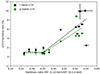 |
Fig. 3. Fractional rms vs hardness ratio calculated as the XRT 2–10 keV / XRT 0.5–2 keV flux and the optical fluxes obtained with LCO in the i′ (black) and g′ (green) bands. Broken power law fits are represented with dashed black and green lines, respectively, to show the increasing trend of the fractional rms with a hardness > 0.35. Results of the fits are reported in Table 2. |
The trend of the optical fractional rms variability amplitude with HRXRT does not follow a simple positive correlation; therefore, we fitted the data using a broken-line model. In the LCO dataset, the fit reveals that, for low values of HRXRT, the slope is close to zero in the i′ and g′ bands. After the break, occurring at HRXRT ∼ 0.35, the data exhibit a strong positive correlation, with Pearson coefficients of 0.77 and 0.84 in the two bands, respectively. We note that HRXRT ≲ 0.35 correspond to MJD ∼58310 − 58380, which, according to the classification by Shidatsu et al. (2019) and Fabian et al. (2020), marks the soft state of the main outburst. Similar trends are seen in the Al Sadeem data, though the break is less well defined due to lower data quality and higher scatter. Fit results are summarised in Table 2.
4.2. X-ray fractional rms amplitude
To reinforce the study of the link between the optical variability and the spectral states, we obtained the fractional rms amplitude in X-rays using Swift/XRT observations in the 2−10 keV energy band. We used two complementary methods. First, we selected specific time-bins to approximate the nominal exposure times of the LCO optical data. We note, however, that the effective time resolution of the optical light curves is coarser (typically ∼150 s) due to filter switching and readout time. From the 5 s, 20 s and 60 s background-subtracted Swift/XRT light curves, we calculated the fractional rms values following the same procedure described for the optical data (Sect. 4.1; Vaughan et al. 2003). Second, event-mode Swift data were analysed in the Fourier domain: Leahy-normalised power-density spectra (PDSs) were computed for each observation segment Leahy et al. (1983), whereas the Poisson-noise contribution was estimated from frequencies in the range of 150−281 Hz and subsequently subtracted. The resulting PDSs were normalised to rms units following van der Klis (1995). Finally, we integrated the variability in the frequency range 0.01−64 Hz (corresponding to ∼0.02 − 100 s).
Figure 4 shows the optical fractional rms measured by LCO in the g′ (green dots) and i′ (black dots) bands plotted against the X-ray fractional rms amplitudes calculated in the 2.0–10.0 keV band for the three different timescales described above: 5 s, 20 s, and 60 s (first three panels, respectively), as well as for the full ∼0.02–100 s range (rightmost panel). We note that the latter was obtained by integrating the PDS over the corresponding frequency range, rather than by binning the light curves.
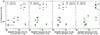 |
Fig. 4. Fractional rms of the optical LCO g′ (green dots) and i′ (black dots) data vs. the Swift/XRT fractional rms amplitude (%) in the 2.0−10.0 keV energy band. The first three panels show the Swift/XRT rms obtained from 5 s-, 20 s-, and 60 s-binned light curves, respectively. The rightmost panel shows the Swift/XRT broadband-frequency rms 0.01−64 Hz (i.e. 0.02–100 s) on the x-axis. Horizontal and vertical error bars represent one-sigma uncertainties calculated analytically for each respective method. |
As the timescale decreases, we observe an increasingly positive correlation between the optical and X-ray rms (despite some scatter), with Pearson coefficients of approximately 0.5 (moderate positive correlation), 0.3, and 0.2 (both weak positive correlations) for the three timescales, respectively. In all cases, the i′-band rms shows a better correlation with the X-ray rms than the g′-band rms. We note that all plots include a clear outlier corresponding to MJD 58305, which falls during the hard-to-soft transition. During this phase, the X-ray rms remains high, while the optical variability appears significantly reduced. This suggests a change in the dominant source of fast optical variability, potentially linked to evolving emission mechanisms during the state transition.
Finally, the optical rms shows a moderate-to-strong positive correlation with the integrated X-ray rms in the 0.01–64 Hz range, with Pearson coefficients of 0.6 and 0.8 in the g′ and i′ bands, respectively. This reflects that the integrated rms provides a reliable estimate of the total X-ray variability, as it encompasses fluctuations across all timescales. The observed correlation with the optical rms may suggest that including intermediate-timescale variations results in a better alignment with the optical response.
5. Short-timescale variability: Discussion
The origin of rapid optical variability in BH LMXBs, observed on sub-second to minute timescales, is a topic of ongoing debate in the astrophysical community. Optical emission in BH binaries can arise from several components, including X-ray reprocessing in the outer disc (e.g. King & Ritter 1998), synchrotron radiation from a compact jet (e.g. Malzac et al. 2018), or from a magnetised hot accretion flow (e.g. Fabian et al. 1982; Veledina et al. 2011), magnetic loop reconnection in the disc (e.g. Zurita et al. 2003). These components can drive variability on different timescales and leave distinct observational signatures, which can help disentangle their relative contributions. Various models have been proposed to explain the complex optical variability observed in BH LMXBs (e.g. Fabian et al. 1982; Merloni et al. 2000; Casella & Pe’er 2009; Veledina et al. 2013; Malzac 2013, 2014; Uttley & Casella 2014; Tetarenko et al. 2021), although few can account for all aspects of variability, including cross-correlation, autocorrelation, and frequency/X-ray state dependence. In the following, we examine some of the possible origins of the variability observed for MAXI J1820+070 during the 2018–2019 outburst.
5.1. Thermal reprocessing
First, we examined whether the observed optical variability could be attributed to X-ray reprocessing. In this scenario, the optical signal represents a delayed and smoothed version of the X-ray variability, shaped by the response of the accretion disc (O’Brien et al. 2002; Vincentelli et al. 2020). In the frequency domain, this leads to a modification of the X-ray variability amplitude depending on the transfer function of the disc (Hynes 2005; Hynes et al. 2006; Veledina et al. 2017). The amplitude of the reprocessed emission is expected to be inversely proportional to the area of its production. Given the large extent of the optically emitting regions of the disc (≈1–10 light seconds; see e.g. O’Brien et al. 2002; Hynes 2005; Hynes et al. 2006), the reprocessed amplitude is seen to be much lower (more than an order of magnitude in fractional units, i.e. never beyond 10%) than the driving one (see Gandhi et al. 2010 for the BH LMXB GX 339-4, or Vincentelli et al. 2020, 2023 for the case of neutron star LMXBs).
Since rms variability is computed over a specific frequency range, it is important to apply the same frequency interval when comparing optical and X-ray rms values. In our case, the frequency range probed by the optical data is constrained by the time resolution and total duration of the observations. Because most observations alternate between g′ and i′ filters and include CCD readout times, the effective time resolution is more than twice the exposure time. For example, in the frequent cases in which we have 16 data points per filter over 40 minutes (Table A.1), the optical data probe variability in the frequency range of approximately 4.2 × 10⁻⁴ to 6.7 × 10⁻³ Hz. This constraint limits our comparison to the third panel of Fig. 4. In that panel, the optical rms is substantially higher than predicted by a reprocessing-only scenario. In some epochs, the optical rms even exceeds the X-ray rms, indicating that additional components beyond thermal reprocessing must contribute to the observed optical variability. It is also worth noting that quasi-periodic oscillations (QPOs) were reported during the hard state, at both optical and X-ray wavelengths (Paice et al. 2021; Mao et al. 2022; Fiori et al. 2025). QPO frequencies as low as ∼50 mHz were reported (periods of ∼20 sec), so variability from these QPOs could contribute to the rms variability, although no obvious QPOs are present by inspecting the light curves (Fig. 6). The optical QPOs were sharper (had lower FWHMs) than X-rays QPOs (Mao et al. 2022), so the optical QPOs cannot be due to reprocessing. In addition, longer timescale oscillations were reported on timescales close to the orbital period (Thomas et al. 2022; Fiori et al. 2025), which were interpreted as high amplitude super-humps from a warped outer disc. Some of the slow trends seen in our light curves around the hard-to-soft transition and in the hard state could be due to sampling of a small part of these modulations.
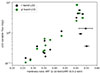 |
Fig. 5. Absolute rms evaluated for LCO i′- and g′-band observations vs hardness of the X-ray spectrum, evaluated using the two Swift/XRT energy bands (2–10 for hard; 0.5–2 for soft). |
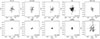 |
Fig. 6. Short-timescale magnitude–magnitude diagrams for MAXI J1820+070 across different phases of its outburst. Each panel shows g′ vs. i′ magnitudes for a specific MJD (indicated in the lower-right corner), with point-to-point connections highlighting the light curve evolution. The different phases of the outburst are indicated on top of each panel, reflecting the spectral state inferred from simultaneous X-ray monitoring. |
We also constructed an absolute rms spectrum by multiplying the fractional rms variability by the average de-reddened flux in the two available bands. The resulting correlation with the X-ray hardness ratio (HRXRT) is shown in Fig. 5. Both bands display a strong and comparable correlation with X-ray spectral hardness, apart from a few outliers. These may correspond to hard-state observations at relatively low luminosities, where the fractional rms remains high (typically 5 − 10%), but the absolute flux is low. Given that the hard state extends down to quiescence, such cases are expected, especially since our dataset includes only limited coverage at these lower luminosities. The spectrum of the variable optical emission does not exhibit a blue shape, which argues against a thermal origin such as disc reprocessing. Instead, the observed properties are more consistent with a non-thermal origin, such as synchrotron emission. In BH LMXBs, synchrotron radiation can originate either from a compact, magnetised hot flow (Veledina et al. 2013) or from a collimated relativistic jet (Malzac 2014). In the following, we examine these two scenarios in the context of the results presented in Sect. 4 for MAXI J1820+070.
5.2. Synchrotron emission from a compact jet
In BH LMXBs, a coupling between accretion and ejection has been shown to occur (Merloni et al. 2003; Falcke et al. 2004; Plotkin et al. 2013), with matter ejected primarily through compact, collimated jets launched near the BH. In the hard X-ray state, a flat radio spectrum typically indicates a jet (Fender 2001, 2004; Corbel et al. 2004). This flat or inverted spectrum (α ∼ 0 to 0.5, with Fν ∝ να) often extends to the infrared (e.g. Corbel & Fender 2002; Gandhi et al. 2011; Rout et al. 2021; Saikia et al. 2019) and results from overlapping self-absorbed synchrotron components at different distances from the BH.
At higher frequencies (infrared to optical), the jet emits optically thin synchrotron radiation after a spectral break, producing a steeper spectrum (−1 < α < −0.5; Buxton & Bailyn 2004; Gandhi et al. 2011; Russell et al. 2013b). This appears as an infrared excess above the extrapolated disc emission and is often highly variable (Casella et al. 2010; Chaty et al. 2011), with fractional rms amplitudes up to about 20 per cent on timescales of seconds to minutes (e.g. GX 339-4 and MAXI J1535-571; Gandhi et al. 2011; Cadolle Bel et al. 2011; Baglio et al. 2018b).
Baglio et al. (2018b) show that the MIR variability in MAXI J1535−571 is consistent with the internal shock model (Malzac 2013, 2014), where variability in the accretion flow creates velocity fluctuations in shells of plasma in the jet, which then collide, generating shocks within the jet. These shocks accelerate particles and produce rapidly varying synchrotron emission. Jet internal shock models (Jamil et al. 2010; Malzac 2013) have also been used to explain the broadband (radio to optical–IR) spectral energy distributions (SEDs) and/or fast timing properties (including lags with the X-ray flux) of GX 339–4 (Drappeau et al. 2015; Malzac et al. 2018), MAXI J1836–194 (Péault et al. 2019) and GRS 1716−249 (Bassi et al. 2020). In addition to strong variations on minute to hour timescales down to sub-second timescales, the jet internal shock model also predicts a ∼0.1 s optical–IR lag with respect to X-ray variability (Malzac et al. 2018), which has been seen in both IR–X-ray and optical–X-ray cross correlations from several BH LMXBs (Gandhi et al. 2008, 2010, 2017; Casella et al. 2010; Paice et al. 2019; Ulgiati et al. 2024).
During the soft X-ray state, jets appear quenched across all wavelengths (e.g. Gallo et al. 2003; Homan et al. 2005; Baglio et al. 2018b). There is evidence that the jet spectral break shifts from IR to radio frequencies during the hard-to-soft transition, and vice versa during the return to the hard state (Coriat et al. 2009; Corbel et al. 2013; Russell et al. 2013b, 2020), with the jet break frequency correlating with the X-ray hardness (Koljonen et al. 2015; Echiburú-Trujillo et al. 2024). The amplitude of the fade/recovery of the IR excess is related to the system inclination, implying that the compact jets are outflowing with Lorentz factors ∼1.3–3.5 (Saikia et al. 2019) and at the peak of the hard state, the jet contributes ∼90 per cent and ∼50 per cent of the NIR and optical flux, respectively (Russell et al. 2006).
In MAXI J1820, a prominent IR excess was seen in the hard state (both before and after the soft state; Russell et al. 2018; Özbey Arabacı et al. 2022; Echiburú-Trujillo et al. 2024), and the IR flux was shown to have stronger variations on sub-seconds to minute timescales than the optical flux (Tetarenko et al. 2021). The power spectral density smoothly evolves from optical to radio wavelengths, with a tight correlation between the break in the power spectrum, and the observational frequency (Tetarenko et al. 2021). This variability is consistent with internal shocks in the jet, from optical to radio, and the PDS break is related to the distance downstream in the jet (Tetarenko et al. 2021). The ∼0.1 sec optical lag commonly attributed to the jet was also reported, with the lag increasing slightly with optical wavelength (Paice et al. 2019, 2021).
Figures 2 and B.1 show that optical minute-timescale variability increases with X-ray hardness, likely indicating a stronger contribution from the jet during harder states. In the LCO data, this is particularly clear in the i′ band, suggesting that the variable component is more prominent at longer wavelengths. This is also supported by Fig. 6, where consecutive g′- and i′-band magnitudes are shown for different outburst stages. Since most observations were composed of consecutive, alternating exposures in the g′ and i′ bands, it was possible to match adjacent magnitudes to see if g′ and i′ magnitudes are correlated, and to compare their variability amplitudes. In the hard state, the distribution of magnitudes has an oval shape, with stronger variability in the i′ band and no clear correlation between the two bands. This pattern is consistent with rapid, flickering-like variability on timescales shorter than the filter-switching cadence of ∼2–3 minutes.
At the hard-to-soft state transition, the variability amplitude decreases and the g′ and i′ magnitudes begin to rise together. In the soft state, the two bands are well correlated (e.g. on MJD 58310 and 58350), although the fractional rms is low (typically below 1–2 per cent), and the variations seem to be dominated by long-term trends, rather than short-term flickering (Fig. A.1). This is in line with expectations for a disc-dominated emission scenario.
Figure 4 shows a positive correlation between the optical and X-ray fractional rms, which is stronger for shorter X-ray binning (5 s). The correlation weakens significantly at longer binning (60 s), where the X-ray rms flattens below 10 per cent. This suggests that the strongest X-ray variability occurs on short timescales. The link between short-timescale variability in the optical and in the emission of the corona, both of which increase with spectral hardness, supports a linked origin. According to the internal shock model, variability in the emission of the corona can introduce velocity fluctuations that generate internal shocks in the jet. These would then produce fast synchrotron variability in the optical, particularly in the i′ band where the jet is expected to contribute more strongly, due its red (optically thin) spectrum, and the bluer disc emission becoming progressively stronger at shorter wavelengths.
In the soft state, the suppression of the jet leads to minimal minute-timescale variability, as observed. In addition to the lower amplitude, the variability becomes slower and better correlated between the g′ and i′ bands. This is consistent with low-level disc fluctuations or reprocessing of X-ray radiation in the extended outer disc (Shidatsu et al. 2019).
To explore this further, we examined the g′−i′ colour as a function of X-ray hardness (Fig. 7). The system remains consistently blue (g′−i′≲0.1) during the soft state and state transitions (Shidatsu et al. 2019; Fabian et al. 2020), in line with expectations for a disc-dominated emission scenario. During harder epochs (HRXRT ≳ 0.4), the colour becomes more variable, with both blue and red values observed. Redder colours tend to appear at low optical fluxes, which also correspond to the hard state. While there is no global trend, the soft and hard states display clearly distinct colour behaviour. In the hard state, the variability is dominated by fluctuations on shorter timescales than the filter switching (Fig. 6), resulting in uncorrelated g′ and i′ magnitudes, and hence, highly variable g′−i′ colours.
The optical fractional rms variability is greater than a few per cent in all hard state observations (including the re-brightening in 2019; Fig. 1 and below 1–2 per cent in the soft state. The highest rms (5–10 per cent) was recorded during the first ∼40 days in the initial hard state, and during the decaying hard state after the soft state. Interestingly, these were epochs when the jet spectral break was at the highest frequencies (> 5 × 10¹² Hz), with the most prominent IR excess (Echiburú-Trujillo et al. 2024). The persistent blue colour during the soft and transition states is consistent with the quenching of the jet, as reported by Echiburú-Trujillo et al. (2024). The hard-to-soft transition, which occurred between MJD 58303.5 and 58310.7 (Yang et al. 2025) and during which the radio jet quenched (Bright et al. 2020), also coincides with a drop in optical g′−i′ colour and variability in our data (orange points in Fig. 7), reinforcing the idea that suppression of the jet leads to reduced optical variability.
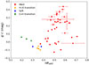 |
Fig. 7. HRXRT vs. g′−i′ colour from the LCO monitoring. Different X-ray spectral states are indicated with different colours following the classification of Shidatsu et al. (2019) and Fabian et al. (2020). |
These results suggest that the observed minute-timescale optical variability originates from the jet in the hard state. When the jet is quenched, such variability disappears, and the low residual variability may reflect slow disc fluctuations. This interpretation is further supported by the optical–X-ray fractional rms correlation, particularly in the i′ band. The positive correlation implies that the variable optical component is stronger at longer wavelengths, consistent with jet-dominated synchrotron emission.
This scenario also provides a natural explanation for the outlier observed on MJD 58305 in the rms correlation plot (lower-right points in Fig. 4). This date corresponds to the hard-to-soft transition, when the jet is believed to have been quenched (Bright et al. 2020). Although the X-ray fractional rms remains elevated, indicating ongoing variability in the emission of the corona, the optical rms drops sharply. If the jet dominates fast optical variability in the hard state, its suppression would lead to a breakdown in this correlation.
Overall, our results support a picture in which the jet plays a dominant role in producing fast optical variability during the hard state, while the soft state is characterised by stable disc emission, in line with expectations for a disc-dominated emission scenario. This is consistent with previous optical/X-ray studies of this source, whereby the jet was claimed to make a contribution to the optical flux (Shidatsu et al. 2018, 2019; Yang et al. 2025; Bright et al. 2025) and variability (Paice et al. 2019, 2021; Tetarenko et al. 2021) in the hard state. The optical fractional rms correlates well with the jet emission in the IR. The smoothly evolving power spectral shape from optical to radio (Fig. 5 in Tetarenko et al. 2021), where the break in the PDS correlates very well with frequency, was measured on MJD 58220, when our rms was ∼5–6 per cent (∼20 per cent rms was measured at optical wavelengths, integrated over all timing frequencies, by Tetarenko et al. 2021). This shows that the majority of the variability (over all timescales) is produced by the jet, at least on that particular date in the hard state.
5.3. The hot magnetised inflow
To account for the complex phenomenology observed in BH LMXBs, including rapid variability across OIR to X-ray wavelengths, inter-band correlations, and broadband spectral behaviour, a modification to the standard thin accretion disc model has been proposed. This framework introduces a radiatively inefficient, magnetised, synchrotron-emitting hot flow that occupies the innermost regions of the accretion geometry, extending inwards towards the BH, potentially down to the innermost stable circular orbit (Veledina et al. 2013). The SED of this hot accretion flow, and any advection-dominated accretion flow or radiatively inefficient accretion flow in the OIR ranges depends sensitively on the radial profiles of key physical quantities, such as the magnetic field strength and electron density (Esin et al. 1997; Blandford & Begelman 1999). The inclusion of non-thermal electrons, as incorporated in hybrid numerical models of hot flows (e.g. Poutanen & Veledina 2014), further modifies the emitted spectrum, typically hardening the OIR SED slope and extending emission to higher energies.
In this scenario, the lower-energy cutoff of the synchrotron spectrum marks the outer boundary of the hot flow (often of the order of several hundred gravitational radii) and typically falls within the OIR domain. At higher energies, in the ultraviolet and optical bands, the spectrum transitions from partially self-absorbed synchrotron to optically thin synchrotron, and eventually to a Comptonised component. It has been suggested that this hot flow could make a substantial contribution from the IR to X-ray flux, particularly during the hard state (Veledina et al. 2013), although the standard accretion disc is still expected to dominate at optical to UV wavelengths.
A feature of the hot flow model is its prediction for short-timescale variability: optical/NIR photons generated by the synchrotron process in the hot inner flow are expected to be anti-correlated with X-ray fluctuations, due to a spectrum that pivots in the UV (Veledina et al. 2011). Here, X-rays arise via Compton upscattering by the same population of hot electrons that produce the optical emission. An increasing mass accretion rate results in brighter X-rays, and reduced optical synchrotron emission due to the increased synchrotron self-absorption. This leads to a characteristic anti-correlation and time delay, with X-ray flares lagging optical dips, and was developed to account for the ‘precognition dip’ in the optical/X-ray cross-correlation function (CCF; Veledina et al. 2011), a feature that had already been explained by a jet ‘energy reservoir’ model (Malzac et al. 2004). Such lag signatures contrast with those expected from standard reprocessing, in which optical–IR fluctuations would be produced by a smeared, lagged response to X-rays variations (O’Brien et al. 2002; Hynes 2005).
While the hot flow could produce detectable synchrotron emission at optical wavelengths, its spectrum is expected to be flat, α ∼ 0 ± 0.5, and become fainter at longer wavelengths into the IR (Veledina et al. 2013). The observed optical–IR flux spectrum in the hard state is red (α ≪ 0; Echiburú-Trujillo et al. 2024), with a peak of the flux density in the MIR. The MIR excess and red SED would imply a very large inner disc truncation radius and challenge the hot flow scenario. The optical rms variability is highest when the MIR is most prominent (Sect. 5.2). The variability properties, in particular the fractional rms and the frequency of the break in the PDS, correlates extremely well with wavelength, from optical to radio (Tetarenko et al. 2021). Since the above observational constraints are inconsistent with expectations for the hot flow, it seems unlikely that this component is responsible for the optical rms variability reported in this work.
Paice et al. (2019, 2021) studied the evolution of the optical/X-ray CCFs using simultaneous data of MAXI J1820 in the initial hard state (MJD 58193–58276). They found that during this time, a sharp ∼0.1 sec lag and a precognition dip were superimposed in the CCFs, and red flares were observed. The ∼0.1–0.2 sec lag, which has been established as a feature of optical–IR jet emission (Gandhi et al. 2017), was strong near the peak of the outburst and weakened later in the hard state. The lag increased at longer optical wavelengths, which is consistent with those longer wavelengths originating from distances further out in the jet, and the progression of matter producing shorter then longer wavelength emission (Paice et al. 2021). The precognition dip, which could be caused by the hot flow, became more prominent during later stages in the hard state, and became broader and shifted to positive lags (optical dips lagging X-ray flares). A model was able to reproduce the CCFs, QPOs and phase lags if the jet dominates the variability at the lowest (< 0.1 Hz) and the highest (> 1 Hz) frequencies, with the hot flow contributing in between (Paice et al. 2021). This is consistent with the findings of Tetarenko et al. (2021), which found the integrated variability (over short and long timescales) increases at longer wavelengths and so has a jet origin, and with the rms variability reported in this work, which is red, and probes relatively long (approximately minute) timescales (< 0.01 Hz). In the Paice et al. (2021) model, the hot flow made a stronger contribution to the (anti-correlated) variability after MJD ∼58225, which is roughly when our rms variability drops below ∼5 per cent. This residual, low-level optical variability could therefore be attributed to cyclo-synchrotron emission from the hot flow.
5.4. Low-flux variability
In Fig. 8 we show the fractional rms variability as a function of magnitude in the g′ and i′ bands. The magnitudes have been averaged over closely spaced epochs and matched to the rms measurements at the nearest MJDs. As the source faded during outburst decay, the fractional rms variability decreases with increasing flux (i.e. decreasing magnitude). However, we observe a striking increase in the optical variability at very low fluxes, corresponding to the (nearly) quiescent state.
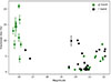 |
Fig. 8. Fractional rms variability as a function of magnitude in the LCO g′ and i′ bands (green and black points, respectively). |
In particular, the g′-band rms reaches values above 20% at magnitudes ≳18, indicating significant variability in the optical even when the source is less active. This level of quiescent optical variability is reminiscent of the behaviour reported for the BH LMXB Swift J1357.2–0933, which exhibited large-amplitude, short-timescale flares in quiescence (Shahbaz et al. 2013). In both cases, the high rms suggests that the emission mechanism in quiescence is dominated by a highly variable component, possibly synchrotron radiation from a weak jet or magnetic reconnection events in the accretion flow.
6. Optical spectroscopy
MAXI J1820+070 was observed spectroscopically with the Cassini 1.5 m telescope at the Loiano Astronomical Observatory (Italy) using the Bologna Faint Object Spectrograph & Camera (BFOSC8) instrument on June 8 (MJD 58277), July 17 (MJD 58316), July 18 (MJD 58317), and November 9, 2018 (MJD 58431), as well as on September 20, 2019 (MJD 58746). Observations were also acquired with the 2.1m telescope of the Observatorio Astrofísico Guillermo Haro (OAGH) in Cananea (Mexico), using a Boller & Chivens spectrograph, on April 15, 2018 (MJD 58223), and with the 2.1 m telescope at the Observatorio Astronómico Nacional San Pedro Mártir (OAN-SPM; Mexico), also equipped with a Boller & Chivens spectrograph, on August 8, 2018 (MJD 58338). Exposure times ranged from 180 to 1800 s. A log of the observations is reported in Table D.1
The BFOSC spectra were acquired with the Grism #4 and a slit width of 2″, providing a nominal spectral coverage of the 3500–8500 Å range and a resolution of ∼10 Å; the OAGH spectra were secured with a 150 lines/mm grating and a slit width of 300 μm (∼2 5), affording a resolution of ∼15 Å in the 3600–7300 Å range, whereas the OAN-SPM ones were secured with a 300 lines/mm grating, a slit width of 2
 5 and a resolution of ∼8 Å, covering the wavelength range between 3700 and 8400 Å.
Data reduction was carried out using standard procedures for both bias subtraction and flat-field correction with IRAF9, and the spectra were optimally extracted according to the procedure of Horne (1986). The wavelength calibration was carried out with helium-argon (Cassini and OAGH data) or neon-helium-copper-argon (OAN-SPM) lamps. The flux calibration was performed using catalogued spectroscopic standard stars within IRAF.
In line with previous spectroscopic works on this source (Tucker et al. 2018; Muñoz-Darias et al. 2019; Sánchez-Sierras & Muñoz-Darias 2020), all of our spectra exhibit numerous emission lines, featuring the Balmer series along with multiple He I and He II transitions (Fig. D.1). Following a visual inspection of all the observing epochs, we focused our analysis on the best spectrum taken during the hard state, during the second re-brightening, which suggests the presence of both disc and wind components.
6.1. Wind signatures during the second re-brightening
Figure 9 shows in detail the average spectrum taken during the second re-brightening, on September 20, 2019 (MJD 58746). This is the best quality spectrum that we obtained while the source was in the hard state, due to the large exposure time (the spectrum is the average of three 1800s spectra; Table D.1). This is the only epoch in which both the Hα and Hβ lines are distorted (i.e. they show a redshifted core; see the inset in Fig. 9), as was observed in the hard state of the main outburst (e.g. Muñoz-Darias et al. 2019), sometimes simultaneously with P-Cyg profiles in other transitions. In the same way as P-Cyg line profiles, these distorted (redshifted) profiles can result from partial absorption of the blue part of the emission component, but in this case the absorption is not strong enough to significantly dip below the continuum level. Our soft-state spectra do not show such signatures, in agreement with Muñoz-Darias et al. (2019), and instead exhibit symmetric, double-peaked profiles. Furthermore, we notice the presence of a possible absorption trough in the blue wing of the Hα line (see the inset in Fig. 9). The velocity associated with this trough is unconstrained, especially considering that broad absorption components are also present (see Sect. 6.2). However, it seems broadly consistent with the wind velocity measured in the past (∼1200–1800 km/s; blue and dashed-dotted red lines in the inset of Fig. 9; Muñoz-Darias et al. 2019; Sánchez-Sierras & Muñoz-Darias 2020).
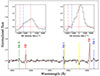 |
Fig. 9. Full normalised spectrum acquired on September 20, 2019, during the hard X-ray spectral state. The position of some of the most relevant emission lines is highlighted with dashed blue (He I 5876 Å and 6678 Å), red (Hα and Hβ), and green (He II) lines. The Na interstellar doublet is marked in yellow. The two insets show zoomed-in views of the normalised spectrum in velocity scale for the Hβ and Hα lines; dotted-dashed blue lines provide the wind velocities measured in the system in previous studies. |
Cold winds in MAXI J1820+070 were first clearly identified during the hard state of the 2018 main outburst through high-resolution spectroscopy by Muñoz-Darias et al. (2019). These features were absent in the soft state, though a NIR wind was later reported by Sánchez-Sierras & Muñoz-Darias (2020). Similar low-ionisation winds have been observed in several other BH LMXBs, including V404 Cyg (Muñoz-Darias et al. 2016), V4641 Sgr (Muñoz-Darias et al. 2018), GRS 1716–249 (Cúneo et al. 2020), MAXI J1803–298 (Mata Sánchez et al. 2022), and MAXI J1348–630 (Panizo-Espinar et al. 2022), suggesting that they are a common feature of BH accretion. Perhaps as a result of our limited spectral resolution, definitive signatures of optical–NIR winds (e.g. P-Cygni profiles) are not clearly resolved in our data. However, the distorted profiles observed in Hα and Hβ suggest that cold winds were likely present during this re-brightening (see also Sánchez-Sierras & Muñoz-Darias 2020), strengthening the case for the presence of these outflows during low-luminosity hard states. This further supports the scenario in which jets and winds can coexist in X-ray binaries.
On the other hand, the absence of obvious wind signatures in our soft-state spectra may instead reflect higher ionisation in the accretion disc, which would suppress low-ionisation features in this phase (see also Muñoz-Darias et al. 2019). To investigate this possibility, we examined the ratio between the equivalent widths of the He II 4686 Å and Hα emission lines as a function of the hardness ratio HRBAT/MAXI. This ratio is systematically higher during soft states compared to hard states, consistent with enhanced disc ionisation. However, systematic effects may contribute, and repeating the analysis with Hβ in place of Hα did not reveal a similar correlation, likely due to the larger uncertainties affecting the Hβ equivalent width measurements.
6.2. Additional spectral features during the reflare
In addition to the aforementioned distorted emission profiles, broad absorptions components are found underlying the emission lines in the spectrum (Hα, Hβ, and He I). Such features are not uncommon and have been observed, typically at low luminosity, in other systems. While their origin is unclear, they might be related to the disc becoming optically thick and behaving like a stellar atmosphere (see e.g. Jiménez-Ibarra et al. 2019; Dubus et al. 2001, and references therein). Finally, He I lines are double-peaked, suggesting for their origin in the accretion disc. The He I 5876 Å line looks blueshifted, but this effect could be due to the presence of the Na interstellar doublet rather than to the presence of an outflow. He I 6678 Å is symmetric, broad and double-peaked, as expected for an accretion disc origin.
7. Conclusions
In this work we present the results of an optical campaign performed on the BH LMXB MAXI J1820+070 during its main 2018 outburst and the following re-brightenings. The campaign involved a systematic photometric monitoring with the telescopes of the LCO network and the telescope of the Al Sadeem Observatory in the UAE, together with low-resolution spectroscopy performed across different spectral states in the same time window using the 2.1 m telescope at the OAN-SPM, the 2.1 m telescope of the OAGH in Cananea (Mexico), and the 1.5 m G.D. Cassini telescope of the Loiano Astronomical Observatory (Italy). Within the photometric monitoring, we specifically focused on time-resolved light curves obtained intermittently throughout the source active period, with a timescale of ∼1 minute. Our main results are as follows.
-
The minute-timescale optical light curves vary substantially depending on the X-ray spectral state. By evaluating the hardness ratio using the Swift/BAT count rate for the hard band and the MAXI count rate for the soft band, we find a strong positive correlation between the hardness ratio and the optical fractional rms, with the latter increasing with hardness, especially at lower optical frequencies. Similarly, we observe a strong positive correlation between the optical fractional rms and the hardness ratio (calculated as the 2–10 keV to 0.5–2 keV Swift/XRT count rate) but only when the hardness ratio exceeds ∼0.35. These findings suggest that variable synchrotron emission from the compact jet drives the observed strong minute-timescale variability. According to accretion-ejection coupling, the jet contributes variable emission during hard states, while it is quenched in soft states.
-
We show that there is a strong correlation between the optical fractional rms and the 0.01–64 Hz Swift/XRT fractional rms amplitude evaluated in the 2–10 keV energy range. This correlation is particularly strong for the optical i′ band. This result is in agreement with the jet scenario, and in particular with the internal shock model (Malzac 2013, 2014), according to which a variable accretion flow is responsible for injecting velocity fluctuation at the base of the jet; this produces shocks that generate variable synchrotron emission in the jet, observable in infrared and optical light curves at different timescales (from sub-seconds to minutes). In the dimmest hard states, the residual very low-level optical variability could instead be attributed to cyclo-synchrotron emission from the hot flow, consistent with the results of Paice et al. (2021).
-
Our low-resolution optical spectroscopy did not reveal clear signs of winds, such as line asymmetries or P-Cygni profiles. Some hard-state spectra show hints of P-Cygni profiles, though none appear in the soft-state spectra. This aligns with previous findings on the source and further supports the presence of optical winds during hard states in MAXI J1820+070. The absence of optical wind signatures in soft states could be related to an over-ionisation of the outflow, as suggested by the positive correlation between the ratio of the equivalent widths of the He II 4686 Å and Hα emission lines and the X-ray hardness.
Data availability
Figure 1 (upper panel) and the reduced spectra presented in this work (Table D.1) are https://cdsarc.cds.unistra.fr/viz-bin/cat/J/A+A/704/A198
MIDAS (Munich Image Data Analysis System) is developed, distributed and maintained by ESO and is available at http://www.eso.org/projects/esomidas/
IRAF is the Image Analysis and Reduction Facility made available to the astronomical community by the National Optical Astronomy Observatories, which are operated by AURA, Inc., under contract with the U.S. National Science Foundation. It is available at https://iraf.noirlab.edu
Acknowledgments
We thank the referee for valuable comments which helped improving our manuscript. We thank Daniel Bramich for valuable discussions on variability estimates and for developing the XB-NEWS pipeline, on whose results this work is based. We moreover thank Silvia Galleti, Ivan Bruni, Antonio De Blasi and Roberto Gualandi of the Loiano Observatory for the assistance at the telescope. MCB is supported by the INAF-Astrofit fellowship. FMV is supported by the European Union’s Horizon Europe research and innovation programme with the Marie Skłodowska-Curie grant agreement No. 101149685. KA, DMR, SR and PS are supported by Tamkeen under the NYU Abu Dhabi Research Institute grant CASS. NM acknowledges financial support through ASI-INAF 2017-14-H.0 agreement (PI: T. Belloni). T.M.-D. acknowledges support by the Spanish Agencia estatal de investigación via PID2021-124879NB-I00. This publication is based on data collected at the Observatorio Astrosico Guillermo Haro (OAGH), Cananea, Sonora, México, operated by the Instituto Nacional de Astrofísica, Óptica y Electrónica (INAOE). This paper is based upon observations carried out at the Observatorio Astronómico Nacional on the Sierra San Pedro Mártir (OAN-SPM), Baja California, México.
References
- Adachi, R., Murata, K. L., Oeda, M., et al. 2020, ATel, 13502, 1 [NASA ADS] [Google Scholar]
- Atri, P., Miller-Jones, J. C. A., Bahramian, A., et al. 2020, MNRAS, 493, L81 [CrossRef] [Google Scholar]
- Baglio, M. C., Russell, D., Qaissieh, T. A., et al. 2018a, ATel, 12128, 1 [Google Scholar]
- Baglio, M. C., Russell, D. M., Casella, P., et al. 2018b, ApJ, 867, 114 [NASA ADS] [CrossRef] [Google Scholar]
- Baglio, M. C., Russell, D. M., & Lewis, F. 2018c, ATel, 11418, 1 [Google Scholar]
- Baglio, M. C., Russell, D. M., Qaissieh, T. A., et al. 2019, ATel, 12596, 1 [Google Scholar]
- Baglio, M. C., Homan, J., Russell, D. M., et al. 2021a, ATel, 14582, 1 [Google Scholar]
- Baglio, M. C., Russell, D. M., Saikia, P., Bramich, D. M., & Lewis, F. 2021b, ATel, 14492, 1 [Google Scholar]
- Baglio, M. C., Russell, D. M., Alabarta, K., et al. 2023, ATel, 16192, 1 [Google Scholar]
- Bahramian, A., Motta, S., Atri, P., & Miller-Jones, J. 2019, ATel, 12573, 1 [Google Scholar]
- Banerjee, S., Dewangan, G. C., Knigge, C., et al. 2024, ApJ, 964, 189 [NASA ADS] [CrossRef] [Google Scholar]
- Bassi, T., Malzac, J., Del Santo, M., et al. 2020, MNRAS, 494, 571 [Google Scholar]
- Belloni, T. M., & Motta, S. E. 2016, in Astrophysics of Black Holes: From Fundamental Aspects to Latest Developments, ed. C. Bambi, Astrophysics and Space Science Library, 440, 61 [NASA ADS] [CrossRef] [Google Scholar]
- Bertin, E., & Arnouts, S. 1996, A&AS, 117, 393 [NASA ADS] [CrossRef] [EDP Sciences] [Google Scholar]
- Blandford, R. D., & Begelman, M. C. 1999, MNRAS, 303, L1 [NASA ADS] [CrossRef] [Google Scholar]
- Bramich, D. M., & Freudling, W. 2012, MNRAS, 424, 1584 [CrossRef] [Google Scholar]
- Bright, J., Motta, S., & Fender, R. 2018a, ATel, 12061, 1 [Google Scholar]
- Bright, J., Motta, S., Fender, R., Perrott, Y., & Titterington, D. 2018b, ATel, 11827, 1 [Google Scholar]
- Bright, J., Motta, S., Williams, D., et al. 2019, ATel, 13041, 1 [Google Scholar]
- Bright, J. S., Fender, R. P., Motta, S. E., et al. 2020, Nat. Astron., 4, 697 [NASA ADS] [CrossRef] [Google Scholar]
- Bright, J., et al. 2025, MNRAS, 541, 1851 [Google Scholar]
- Buxton, M. M., & Bailyn, C. D. 2004, ApJ, 615, 880 [NASA ADS] [CrossRef] [Google Scholar]
- Cadolle Bel, M., Rodriguez, J., D’Avanzo, P., et al. 2011, A&A, 534, A119 [NASA ADS] [CrossRef] [EDP Sciences] [Google Scholar]
- Casella, P., & Pe’er, A. 2009, ApJ, 703, L63 [Google Scholar]
- Casella, P., Maccarone, T. J., O’Brien, K., et al. 2010, MNRAS, 404, L21 [NASA ADS] [Google Scholar]
- Casella, P., Vincentelli, F., O’Brien, K., et al. 2018, ATel, 11451, 1 [Google Scholar]
- Chambers, K. C., Magnier, E. A., Metcalfe, N., et al. 2016, ArXiv e-prints [arXiv:1612.05560] [Google Scholar]
- Chaty, S., Dubus, G., & Raichoor, A. 2011, A&A, 529, A3 [CrossRef] [EDP Sciences] [Google Scholar]
- Chaty, S., Haswell, C. A., Malzac, J., et al. 2003, MNRAS, 346, 689 [Google Scholar]
- Corbel, S., & Fender, R. P. 2002, ApJ, 573, L35 [NASA ADS] [CrossRef] [Google Scholar]
- Corbel, S., Fender, R. P., Tomsick, J. A., Tzioumis, A. K., & Tingay, S. 2004, ApJ, 617, 1272 [CrossRef] [Google Scholar]
- Corbel, S., Aussel, H., Broderick, J. W., et al. 2013, MNRAS, 431, L107 [NASA ADS] [CrossRef] [Google Scholar]
- Coriat, M., Corbel, S., Buxton, M. M., et al. 2009, MNRAS, 400, 123 [Google Scholar]
- Cúneo, V. A., Muñoz-Darias, T., Sánchez-Sierras, J., et al. 2020, MNRAS, 498, 25 [CrossRef] [Google Scholar]
- Denisenko, D. 2018, ATel, 11400, 1 [Google Scholar]
- Díaz Trigo, M., & Boirin, L. 2016, Astron. Nachr., 337, 368 [Google Scholar]
- Drappeau, S., Malzac, J., Belmont, R., Gandhi, P., & Corbel, S. 2015, MNRAS, 447, 3832 [Google Scholar]
- Drappeau, S., Malzac, J., Coriat, M., et al. 2017, MNRAS, 466, 4272 [NASA ADS] [Google Scholar]
- Dubus, G., Kim, R. S. J., Menou, K., Szkody, P., & Bowen, D. V. 2001, ApJ, 553, 307 [NASA ADS] [CrossRef] [Google Scholar]
- Echiburú-Trujillo, C., Tetarenko, A. J., Haggard, D., et al. 2024, ApJ, 962, 116 [Google Scholar]
- Esin, A. A., McClintock, J. E., & Narayan, R. 1997, ApJ, 489, 865 [NASA ADS] [CrossRef] [Google Scholar]
- Espinasse, M., Corbel, S., Kaaret, P., et al. 2020, ApJ, 895, L31 [NASA ADS] [CrossRef] [Google Scholar]
- Ester, M., Kriegel, H. P., Sander, J., & Xu, X. 1996, in Second International Conference on Knowledge Discovery and Data Mining (KDD’96). Proceedings of a conference held August 2–4, eds. D. W. Pfitzner, & J. K. Salmon, 226 [Google Scholar]
- Fabian, A. C., Guilbert, P. W., Motch, C., et al. 1982, A&A, 111, L9 [NASA ADS] [Google Scholar]
- Fabian, A. C., Buisson, D. J., Kosec, P., et al. 2020, MNRAS, 493, 5389 [NASA ADS] [CrossRef] [Google Scholar]
- Falcke, H., Körding, E., & Markoff, S. 2004, A&A, 414, 895 [NASA ADS] [CrossRef] [EDP Sciences] [Google Scholar]
- Fender, R. 2004, New Astron. Rev., 48, 1399 [Google Scholar]
- Fender, R., & Gallo, E. 2014, Space Sci. Rev., 183, 323 [NASA ADS] [CrossRef] [Google Scholar]
- Fender, R. P. 2001, MNRAS, 322, 31 [NASA ADS] [CrossRef] [Google Scholar]
- Fiori, M., Zampieri, L., Burtovoi, A., et al. 2025, A&A, 697, A222 [NASA ADS] [CrossRef] [EDP Sciences] [Google Scholar]
- Gallo, E., Fender, R. P., & Pooley, G. G. 2003, MNRAS, 344, 60 [Google Scholar]
- Gandhi, P., Bachetti, M., Dhillon, V. S., et al. 2017, Nat. Astron., 1, 859 [NASA ADS] [CrossRef] [Google Scholar]
- Gandhi, P., Makishima, K., Durant, M., et al. 2008, MNRAS, 390, L29 [Google Scholar]
- Gandhi, P., Dhillon, V. S., Durant, M., et al. 2010, MNRAS, 407, 2166 [NASA ADS] [CrossRef] [Google Scholar]
- Gandhi, P., Blain, A. W., Russell, D. M., et al. 2011, ApJ, 740, L13 [NASA ADS] [CrossRef] [Google Scholar]
- Gandhi, P., Paice, J. A., Littlefair, S. P., et al. 2018, ATel, 11437, 1 [Google Scholar]
- Goodwin, A. J., Russell, D. M., Galloway, D. K., et al. 2020, MNRAS, 498, 3429 [NASA ADS] [CrossRef] [Google Scholar]
- Hambsch, J., Ulowetz, J., Vanmunster, T., Cejudo, D., & Patterson, J. 2019, ATel, 13014, 1 [NASA ADS] [Google Scholar]
- Henden, A. A., Levine, S., Terrell, D., et al. 2018, Am. Astron. Soc. Meet. Abstr., 232, 223.06 [Google Scholar]
- Homan, J. 2001, PhD thesis, University of Amsterdam, The Netherlands [Google Scholar]
- Homan, J., Buxton, M., Markoff, S., et al. 2005, ApJ, 624, 295 [NASA ADS] [CrossRef] [Google Scholar]
- Homan, J., Uttley, P., Gendreau, K., et al. 2018, ATel, 11820, 1 [Google Scholar]
- Homan, J., Bright, J., Motta, S. E., et al. 2020, ApJ, 891, L29 [NASA ADS] [CrossRef] [Google Scholar]
- Horne, K. 1986, PASP, 98, 609 [Google Scholar]
- Hynes, R. I. 2005, in The Astrophysics of Cataclysmic Variables and Related Objects, eds. J. M. Hameury, & J. P. Lasota, ASP Conf. Ser., 330, 237 [Google Scholar]
- Hynes, R. I., Horne, K., O’Brien, K., et al. 2006, ApJ, 648, 1156 [Google Scholar]
- Jamil, O., Fender, R. P., & Kaiser, C. R. 2010, MNRAS, 401, 394 [Google Scholar]
- Jiménez-Ibarra, F., Muñoz-Darias, T., Casares, J., Armas Padilla, M., & Corral-Santana, J. M. 2019, MNRAS, 489, 3420 [Google Scholar]
- Jordi, K., Grebel, E. K., & Ammon, K. 2006, A&A, 460, 339 [NASA ADS] [CrossRef] [EDP Sciences] [Google Scholar]
- Kara, E., Steiner, J. F., Fabian, A. C., et al. 2019, Nature, 565, 198 [Google Scholar]
- Kawamuro, T., Negoro, H., Yoneyama, T., et al. 2018, ATel, 11399, 1 [Google Scholar]
- Kimura, M., & Done, C. 2019, MNRAS, 482, 626 [Google Scholar]
- King, A. R., & Ritter, H. 1998, MNRAS, 293, L42 [NASA ADS] [CrossRef] [Google Scholar]
- Koljonen, K. I. I., Russell, D. M., Fernández-Ontiveros, J. A., et al. 2015, ApJ, 814, 139 [CrossRef] [Google Scholar]
- Lang, D., Hogg, D. W., Mierle, K., Blanton, M., & Roweis, S. 2010, AJ, 139, 1782 [Google Scholar]
- Leahy, D. A., Darbro, W., Elsner, R. F., et al. 1983, ApJ, 266, 160 [NASA ADS] [CrossRef] [Google Scholar]
- Lewis, F., Russell, D. M., Fender, R. P., Roche, P., & Clark, J. S. 2008, ArXiv e-prints [arXiv:0811.2336] [Google Scholar]
- Malzac, J. 2013, MNRAS, 429, L20 [NASA ADS] [CrossRef] [Google Scholar]
- Malzac, J. 2014, MNRAS, 443, 299 [NASA ADS] [CrossRef] [Google Scholar]
- Malzac, J., Merloni, A., & Fabian, A. C. 2004, MNRAS, 351, 253 [NASA ADS] [CrossRef] [Google Scholar]
- Malzac, J., Kalamkar, M., Vincentelli, F., et al. 2018, MNRAS, 480, 2054 [NASA ADS] [CrossRef] [Google Scholar]
- Mao, D.-M., Yu, W.-F., Zhang, J.-J., et al. 2022, Res. Astron. Astrophys., 22, 045009 [CrossRef] [Google Scholar]
- Marino, A., Malzac, J., Del Santo, M., et al. 2020, MNRAS, 498, 3351 [CrossRef] [Google Scholar]
- Mata Sánchez, D., Muñoz-Darias, T., Cúneo, V. A., et al. 2022, ApJ, 926, L10 [CrossRef] [Google Scholar]
- Merloni, A., Di Matteo, T., & Fabian, A. C. 2000, MNRAS, 318, L15 [NASA ADS] [CrossRef] [Google Scholar]
- Merloni, A., Heinz, S., & di Matteo, T. 2003, MNRAS, 345, 1057 [Google Scholar]
- Motta, S. E., Casella, P., Henze, M., et al. 2015, MNRAS, 447, 2059 [NASA ADS] [CrossRef] [Google Scholar]
- Muñoz-Darias, T., Motta, S., & Belloni, T. M. 2011, MNRAS, 410, 679 [Google Scholar]
- Muñoz-Darias, T., Casares, J., Mata Sánchez, D., et al. 2016, Nature, 534, 75 [Google Scholar]
- Muñoz-Darias, T., Torres, M. A. P., & Garcia, M. R. 2018, MNRAS, 479, 3987 [CrossRef] [Google Scholar]
- Muñoz-Darias, T., Jiménez-Ibarra, F., Panizo-Espinar, G., et al. 2019, ApJ, 879, L4 [CrossRef] [Google Scholar]
- Negoro, H., Nakajima, M., Sakamaki, A., et al. 2018, ATel, 12057, 1 [Google Scholar]
- Neilsen, J., & Degenaar, N. 2023, ArXiv e-prints [arXiv:2304.05412] [Google Scholar]
- O’Brien, K., Horne, K., Hynes, R. I., et al. 2002, MNRAS, 334, 426 [Google Scholar]
- Özbey Arabacı, M., Kalemci, E., Dinçer, T., et al. 2022, MNRAS, 514, 3894 [Google Scholar]
- Paice, J. A., Gandhi, P., Shahbaz, T., et al. 2019, MNRAS, 490, L62 [NASA ADS] [CrossRef] [Google Scholar]
- Paice, J. A., Gandhi, P., Shahbaz, T., et al. 2021, MNRAS, 505, 3452 [NASA ADS] [CrossRef] [Google Scholar]
- Panizo-Espinar, G., Armas Padilla, M., Muñoz-Darias, T., et al. 2022, A&A, 664, A100 [NASA ADS] [CrossRef] [EDP Sciences] [Google Scholar]
- Péault, M., Malzac, J., Coriat, M., et al. 2019, MNRAS, 482, 2447 [CrossRef] [Google Scholar]
- Plotkin, R. M., Gallo, E., & Jonker, P. G. 2013, ApJ, 773, 59 [NASA ADS] [CrossRef] [Google Scholar]
- Ponti, G., Fender, R. P., Begelman, M. C., et al. 2012, MNRAS, 422, 11 [Google Scholar]
- Poutanen, J., & Veledina, A. 2014, Space Sci. Rev., 183, 61 [CrossRef] [Google Scholar]
- Rout, S. K., Vadawale, S. V., Aarthy, E., et al. 2021, J. Astrophys. Astron., 42, 39 [Google Scholar]
- Russell, D. M., Fender, R. P., Hynes, R. I., et al. 2006, MNRAS, 371, 1334 [NASA ADS] [CrossRef] [Google Scholar]
- Russell, D. M., Maitra, D., Dunn, R. J. H., & Markoff, S. 2010, MNRAS, 405, 1759 [NASA ADS] [Google Scholar]
- Russell, D. M., Maitra, D., Dunn, R. J. H., & Fender, R. P. 2011, MNRAS, 416, 2311 [Google Scholar]
- Russell, D. M., Markoff, S., Casella, P., et al. 2013a, MNRAS, 429, 815 [NASA ADS] [CrossRef] [Google Scholar]
- Russell, D. M., Russell, T. D., Miller-Jones, J. C. A., et al. 2013b, ApJ, 768, L35 [NASA ADS] [CrossRef] [Google Scholar]
- Russell, D. M., Baglio, M. C., Bright, J., et al. 2018, ATel, 11533, 1 [Google Scholar]
- Russell, D. M., Baglio, M. C., & Lewis, F. 2019a, ATel, 12534, 1 [NASA ADS] [Google Scholar]
- Russell, D. M., Bramich, D. M., Lewis, F., et al. 2019b, Astron. Nachr., 340, 278 [NASA ADS] [CrossRef] [Google Scholar]
- Russell, T. D., Lucchini, M., Tetarenko, A. J., et al. 2020, MNRAS, 498, 5772 [NASA ADS] [CrossRef] [Google Scholar]
- Saikia, P., Russell, D. M., Bramich, D. M., et al. 2019, ApJ, 887, 21 [NASA ADS] [CrossRef] [Google Scholar]
- Sako, S., Ohsawa, R., Ichiki, M., et al. 2018, ATel, 11426, 1 [Google Scholar]
- Sánchez-Sierras, J., & Muñoz-Darias, T. 2020, A&A, 640, L3 [EDP Sciences] [Google Scholar]
- Sasaki, R., Negoro, H., Nakahira, S., et al. 2020, ATel, 13530, 1 [Google Scholar]
- Shahbaz, T., Russell, D. M., Zurita, C., et al. 2013, MNRAS, 434, 2696 [NASA ADS] [CrossRef] [Google Scholar]
- Shidatsu, M., Nakahira, S., Yamada, S., et al. 2018, ApJ, 868, 54 [CrossRef] [Google Scholar]
- Shidatsu, M., Nakahira, S., Murata, K. L., et al. 2019, ApJ, 874, 183 [NASA ADS] [CrossRef] [Google Scholar]
- Stetson, P. B. 1990, PASP, 102, 932 [Google Scholar]
- Tetarenko, A. J., Casella, P., Miller-Jones, J. C. A., et al. 2021, MNRAS, 504, 3862 [NASA ADS] [CrossRef] [Google Scholar]
- Thomas, J. K., Charles, P. A., Buckley, D. A. H., et al. 2022, MNRAS, 509, 1062 [Google Scholar]
- Tomsick, J. A., & Homan, J. 2019, ATel, 12732, 1 [Google Scholar]
- Tonry, J. L., Denneau, L., Flewelling, H., et al. 2018, ApJ, 867, 105 [NASA ADS] [CrossRef] [Google Scholar]
- Torres, M. A. P., Casares, J., Jiménez-Ibarra, F., et al. 2019, ApJ, 882, L21 [NASA ADS] [CrossRef] [Google Scholar]
- Torres, M. A. P., Casares, J., Jiménez-Ibarra, F., et al. 2020, ApJ, 893, L37 [NASA ADS] [CrossRef] [Google Scholar]
- Trushkin, S. A., Nizhelskij, N. A., Tsybulev, P. G., & Erkenov, A. 2018, ATel, 11439, 1 [Google Scholar]
- Tucker, M. A., Shappee, B. J., Holoien, T. W. S., et al. 2018, ApJ, 867, L9 [NASA ADS] [CrossRef] [Google Scholar]
- Ulgiati, A., Vincentelli, F. M., Casella, P., et al. 2024, A&A, 690, A239 [NASA ADS] [CrossRef] [EDP Sciences] [Google Scholar]
- Ulowetz, J., Myers, G., & Patterson, J. 2019, ATel, 12567, 1 [NASA ADS] [Google Scholar]
- Uttley, P., & Casella, P. 2014, Space Sci. Rev., 183, 453 [NASA ADS] [CrossRef] [Google Scholar]
- van der Klis, M. 1995, X-ray Binaries, 252 [Google Scholar]
- van Paradijs, J., & McClintock, J. E. 1994, A&A, 290, 133 [NASA ADS] [Google Scholar]
- Vaughan, S., Edelson, R., Warwick, R. S., & Uttley, P. 2003, MNRAS, 345, 1271 [Google Scholar]
- Veledina, A., Poutanen, J., & Vurm, I. 2011, ApJ, 737, L17 [NASA ADS] [CrossRef] [Google Scholar]
- Veledina, A., Poutanen, J., & Vurm, I. 2013, MNRAS, 430, 3196 [NASA ADS] [CrossRef] [Google Scholar]
- Veledina, A., Gandhi, P., Hynes, R., et al. 2017, MNRAS, 470, 48 [CrossRef] [Google Scholar]
- Vincentelli, F. M., & Muñoz-Darias, T. 2025, A&A, 695, A181 [NASA ADS] [CrossRef] [EDP Sciences] [Google Scholar]
- Vincentelli, F. M., Casella, P., Petrucci, P., et al. 2019, ApJ, 887, L19 [NASA ADS] [CrossRef] [Google Scholar]
- Vincentelli, F. M., Cavecchi, Y., Casella, P., et al. 2020, MNRAS, 495, L37 [NASA ADS] [CrossRef] [Google Scholar]
- Vincentelli, F. M., Casella, P., Russell, D. M., et al. 2021, MNRAS, 503, 614 [NASA ADS] [CrossRef] [Google Scholar]
- Vincentelli, F. M., Neilsen, J., Tetarenko, A. J., et al. 2023, Nature, 615, 45 [Google Scholar]
- Williams, D., Motta, S., Bright, J., et al. 2019, ATel, 12577, 1 [Google Scholar]
- Xu, Y., Harrison, F., & Tomsick, J. 2019, ATel, 13025, 1 [Google Scholar]
- Yang, P., Zhang, G., Russell, D. M., et al. 2025, A&A, 700, A79 [NASA ADS] [CrossRef] [EDP Sciences] [Google Scholar]
- You, B., Tuo, Y., Li, C., et al. 2021, Nat. Commun., 12, 1025 [NASA ADS] [CrossRef] [Google Scholar]
- Zampieri, L., Munari, U., Ochner, P., & Manzini, F. 2019, ATel, 12747, 1 [Google Scholar]
- Zurita, C., Casares, J., & Shahbaz, T. 2003, ApJ, 582, 369 [NASA ADS] [CrossRef] [Google Scholar]
Appendix A: LCO short-timescale light curves
A selection of short-timescale light curves of MAXI J1820 throughout the 2018-2019 main outburst and reflares are shown in Fig. A.1. Details of the light curves (MJDs, exposure times and telescope configuration) can be found in Table A.1.
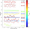 |
Fig. A.1. Selection of short-timescale light curves of MAXI J1820+070 from the campaign presented in this work. The X-ray spectral hardness is colour-coded, as indicated by the colour bar (red is hard, blue is soft). The g′- and i′-band light curves are shown as stars and squares, respectively. Time is measured in minutes since the start of each light curve. |
Fast-timing i′- and g′-band LCO observations published in this work.
Appendix B: Al Sadeem Observatory short-timescale light curves
A complete log of the short-timescale light curves obtained at the Al Sadeem Observatory can be found in Table B.1. In Fig. B.1, the correlation between the fractional rms of the optical light curves and the HR (HRBAT/MAXI and HRXRT) is shown.
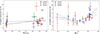 |
Fig. B.1. Top: Fractional rms vs hardness ratio calculated as the BAT flux/MAXI flux and the optical fluxes obtained at the Al Sadeem Observatory in the g′, V, and R bands (blue, green, and red points, respectively). Linear fits are represented with colour-coded dashed lines. Results of the fits are reported in Table 1. Bottom: Fractional rms vs hardness ratio calculated as the 2-10 keV Swift/XRT flux / the 0.5-2 keV Swift/XRT flux and the optical fluxes obtained at the Al Sadeem Observatory in the g′, V, and R bands. Results of the fits are reported in Table 2. |
Fast-timing blue-, green-, and red-band Al Sadeem Observatory observations published in this work.
Appendix C: Hardness-intensity diagrams
In order to observe the evolution of the hardness of the X-ray spectra, we built the hardness-intensity diagram (HID; Homan 2001) of MAXI J1820+070 during the main 2018 outburst, between MJD 58190 and MJD 58420 (that is, March 13, 2018, and October 29, 2018, respectively). To do so, we used data acquired almost daily with Swift/BAT and MAXI in the 15−50 keV and 2−10 keV energy bands, respectively. We converted the fluxes from both Swift/BAT and MAXI into Crab units as described in Sect. 3.3, and we defined the hardness ratio HRBAT/MAXI as the ratio between the flux of Swift/BAT and MAXI in Crab units. For the y-axis of the HID, we used the MAXI flux in Crab units in the 2−10 keV band (Fig. C.1, left panel).
Similarly, we built an HID using the hardness ratio HRXRT, defined as the ratio of the 2−10 keV XRT count rates to the 0.5−2 keV XRT count rates, plotted against the XRT 2−10 keV count rates (Fig. C.1, right panel).
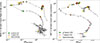 |
Fig. C.1. HID of MAXI J1820+070 during its main 2018 outburst, constructed using HRBAT/MAXI (left) and HRXRT (right) as hardness ratios. Squares indicate epochs where nearly simultaneous (within one day) fractional rms variability amplitudes and hardness ratio estimates were obtained in the g′ (green) and i′ (red) LCO bands. For clarity, the Al Sadeem time-resolved epochs are not shown. Yellow diamonds mark the epochs of the spectroscopic campaign during the main outburst (Sect. 6 and Appendix D), with each point corresponding to the closest hardness ratio measurement to the spectroscopic observation. |
Following the spectral state classification for MAXI J1820+070 described by, for example, Shidatsu et al. (2019) and Fabian et al. (2020), the outburst displayed a standard pattern for a BH LMXB: after an initial stage in the hard state, the system transitioned to a hard intermediate state around MJD 58300 (July 1, 2018), rapidly transitioning to the soft state. The X-ray spectrum remained soft until ∼ MJD 58393 (October 2, 2018), when it started to transition back to the hard state. After the transition to the hard state, the main outburst ended (as can be observed in the first two panels of Fig. 1).
Appendix D: Spectroscopic observations
The collection of spectra described in this work can be found in Fig. D.1. A complete log of the observations is reported in Table D.1. The spectra have been normalised to their local continua in order to facilitate a direct comparison of the line profiles. Although flux standards were observed during the runs, the resulting flux calibration is affected by significant and wavelength-dependent uncertainties (e.g. due to slit losses), and therefore the absolute flux level and continuum shape are not reliable. For this reason, we focus on the normalised spectra throughout the paper. In principle, the continuum shape could provide valuable information on the relative contributions of reprocessing and jet emission (e.g. Kimura & Done 2019), as it may evolve from reprocessing-dominated to jet-dominated regimes. However, the spectral coverage and flux calibration accuracy of our data are insufficient for a reliable analysis of this kind.
Complete log of the spectroscopic observations.
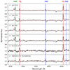 |
Fig. D.1. Averaged spectra collected in the six different epochs reported in this work (Table D.1). The positions of the most prominent He II, H, and He I emission lines are shown with vertical dashed green, red, and blue lines, respectively. A horizontal dashed red line marks where the normalised flux is equal to 1 in each panel. |
All Tables
Results of the correlation study using the hardness ratio calculated as the ratio between the BAT (hard) and the MAXI (soft) X-ray fluxes vs. the optical fractional rms of the LCO g′ and i′ and Al Sadeem g′, V, and R light curves.
Fast-timing blue-, green-, and red-band Al Sadeem Observatory observations published in this work.
All Figures
|
Fig. 1. First panel: optical LCO (g′ and i′) and Al Sadeem (g′, V, and R) light curves of MAXI J1820+070 during its 2018-2019 outburst. Magnitudes are not corrected for reddening. Second panel: Swift/BAT (purple), Swift/XRT (pink), and MAXI/GSC (dark purple) count rates vs MJD. Swift/BAT counts have been divided by 100 for visualisation purposes. Third panel: MJD vs. fractional rms variability amplitude evaluated for the time-resolved optical light curves obtained with the LCO and Al Sadeem observations. Fourth panel: MJD vs. hardness ratio evaluated as BAT/MAXI count rates (HRBAT/MAXI) and XRT (2–10 keV)/XRT (0.5–2 keV) count rates (HRXRT). The first panel is available at the CDS. |
| In the text | |
|
Fig. 2. Hardness ratio (calculated as BAT/MAXI) vs fractional rms of the optical LCO g′ (green dots) and i′ (black dots) data. Linear fits to the data are represented with dashed green and black lines, respectively, to show the increasing trend of the fractional rms with the hardness. |
| In the text | |
|
Fig. 3. Fractional rms vs hardness ratio calculated as the XRT 2–10 keV / XRT 0.5–2 keV flux and the optical fluxes obtained with LCO in the i′ (black) and g′ (green) bands. Broken power law fits are represented with dashed black and green lines, respectively, to show the increasing trend of the fractional rms with a hardness > 0.35. Results of the fits are reported in Table 2. |
| In the text | |
|
Fig. 4. Fractional rms of the optical LCO g′ (green dots) and i′ (black dots) data vs. the Swift/XRT fractional rms amplitude (%) in the 2.0−10.0 keV energy band. The first three panels show the Swift/XRT rms obtained from 5 s-, 20 s-, and 60 s-binned light curves, respectively. The rightmost panel shows the Swift/XRT broadband-frequency rms 0.01−64 Hz (i.e. 0.02–100 s) on the x-axis. Horizontal and vertical error bars represent one-sigma uncertainties calculated analytically for each respective method. |
| In the text | |
|
Fig. 5. Absolute rms evaluated for LCO i′- and g′-band observations vs hardness of the X-ray spectrum, evaluated using the two Swift/XRT energy bands (2–10 for hard; 0.5–2 for soft). |
| In the text | |
|
Fig. 6. Short-timescale magnitude–magnitude diagrams for MAXI J1820+070 across different phases of its outburst. Each panel shows g′ vs. i′ magnitudes for a specific MJD (indicated in the lower-right corner), with point-to-point connections highlighting the light curve evolution. The different phases of the outburst are indicated on top of each panel, reflecting the spectral state inferred from simultaneous X-ray monitoring. |
| In the text | |
|
Fig. 7. HRXRT vs. g′−i′ colour from the LCO monitoring. Different X-ray spectral states are indicated with different colours following the classification of Shidatsu et al. (2019) and Fabian et al. (2020). |
| In the text | |
|
Fig. 8. Fractional rms variability as a function of magnitude in the LCO g′ and i′ bands (green and black points, respectively). |
| In the text | |
|
Fig. 9. Full normalised spectrum acquired on September 20, 2019, during the hard X-ray spectral state. The position of some of the most relevant emission lines is highlighted with dashed blue (He I 5876 Å and 6678 Å), red (Hα and Hβ), and green (He II) lines. The Na interstellar doublet is marked in yellow. The two insets show zoomed-in views of the normalised spectrum in velocity scale for the Hβ and Hα lines; dotted-dashed blue lines provide the wind velocities measured in the system in previous studies. |
| In the text | |
|
Fig. A.1. Selection of short-timescale light curves of MAXI J1820+070 from the campaign presented in this work. The X-ray spectral hardness is colour-coded, as indicated by the colour bar (red is hard, blue is soft). The g′- and i′-band light curves are shown as stars and squares, respectively. Time is measured in minutes since the start of each light curve. |
| In the text | |
|
Fig. B.1. Top: Fractional rms vs hardness ratio calculated as the BAT flux/MAXI flux and the optical fluxes obtained at the Al Sadeem Observatory in the g′, V, and R bands (blue, green, and red points, respectively). Linear fits are represented with colour-coded dashed lines. Results of the fits are reported in Table 1. Bottom: Fractional rms vs hardness ratio calculated as the 2-10 keV Swift/XRT flux / the 0.5-2 keV Swift/XRT flux and the optical fluxes obtained at the Al Sadeem Observatory in the g′, V, and R bands. Results of the fits are reported in Table 2. |
| In the text | |
|
Fig. C.1. HID of MAXI J1820+070 during its main 2018 outburst, constructed using HRBAT/MAXI (left) and HRXRT (right) as hardness ratios. Squares indicate epochs where nearly simultaneous (within one day) fractional rms variability amplitudes and hardness ratio estimates were obtained in the g′ (green) and i′ (red) LCO bands. For clarity, the Al Sadeem time-resolved epochs are not shown. Yellow diamonds mark the epochs of the spectroscopic campaign during the main outburst (Sect. 6 and Appendix D), with each point corresponding to the closest hardness ratio measurement to the spectroscopic observation. |
| In the text | |
|
Fig. D.1. Averaged spectra collected in the six different epochs reported in this work (Table D.1). The positions of the most prominent He II, H, and He I emission lines are shown with vertical dashed green, red, and blue lines, respectively. A horizontal dashed red line marks where the normalised flux is equal to 1 in each panel. |
| In the text | |
Current usage metrics show cumulative count of Article Views (full-text article views including HTML views, PDF and ePub downloads, according to the available data) and Abstracts Views on Vision4Press platform.
Data correspond to usage on the plateform after 2015. The current usage metrics is available 48-96 hours after online publication and is updated daily on week days.
Initial download of the metrics may take a while.