| Issue |
A&A
Volume 704, December 2025
|
|
|---|---|---|
| Article Number | A247 | |
| Number of page(s) | 19 | |
| Section | Planets, planetary systems, and small bodies | |
| DOI | https://doi.org/10.1051/0004-6361/202556730 | |
| Published online | 17 December 2025 | |
Asteroid-GS: 3D Gaussian splatting for fast surface reconstruction of asteroids
1
School of Astronautics, Beihang University, Beijing 100191, China
2
State Key Laboratory of High-Efficiency Reusable Aerospace Transportation Technology, Beijing 102206, China
★ Corresponding authors: This email address is being protected from spambots. You need JavaScript enabled to view it.
Received:
4
August
2025
Accepted:
6
November
2025
Context. Asteroid surface reconstruction is essential for deep space exploration missions, as it provides critical information about surface morphology that supports spacecraft navigation and sample acquisition. Traditional methods, such as stereo-photogrammetry (SPG) and stereo-photoclinometry (SPC), have been widely applied in asteroid missions, which often rely on large amounts of data or considerable manual intervention to derive reliable models. Meanwhile, intelligent methods based on the neural radiance field (NeRF) suffer from slow processing speeds, often requiring several hours or even days to complete surface reconstruction. Recent 3D Gaussian splatting (3DGS) shows promise in fast surface reconstruction but faces some challenges in asteroid scenarios, limiting its direct application.
Aims. This paper presents Asteroid-GS, a fast and intelligent method for reconstructing asteroid surface models based on 3DGS. It is intended to complement current methodologies, enabling asteroid reconstruction with a limited number of images and a small amount of processing time while achieving an accuracy comparable that of to existing algorithms.
Methods. Our method incorporates an adaptive Gaussian pruning strategy to remove noise from asteroids in deep space environments. The shallow multilayer perceptrons integrated with asteroid illumination are employed to improve the reconstruction in both well-lit and shadowed regions. Additionally, we employ geometric regularization techniques to enhance surface detail preservation and construct the Gaussian opacity field to enable accurate surface mesh extraction.
Results. Experimental results on asteroids Itokawa and Ryugu demonstrate that our method outperforms state-of-the-art 3DGS-based methods in terms of 3D model accuracy and novel view synthesis. It maintains geometric consistency with traditional models, achieving better results than SPG given the same input images, while notably reducing processing time and manual intervention compared to SPC. Asteroid-GS completes reconstruction within one hour, requiring significantly less time than NeRF-based methods. Our work provides a supplementary solution for asteroid surface reconstruction, potentially improving the efficiency of future exploration missions.
Key words: techniques: image processing / minor planets, asteroids: general / planets and satellites: surfaces
© The Authors 2025
 Open Access article, published by EDP Sciences, under the terms of the Creative Commons Attribution License (https://creativecommons.org/licenses/by/4.0), which permits unrestricted use, distribution, and reproduction in any medium, provided the original work is properly cited.
This article is published in open access under the Subscribe to Open model. This email address is being protected from spambots. You need JavaScript enabled to view it. to support open access publication.
1 Introduction
Asteroid exploration is vital for understanding the evolution of the Solar System, as well as defending against potential asteroid impacts (Chapman & Morrison 1994). The precise shape of an asteroid provides key insights into its formation, geology, and evolution. Additionally, it enables the accurate determination of the asteroid’s volume, which helps in estimating its mass density. These scientific and practical motivations have led various countries to launch a series of asteroid exploration missions over the years, beginning in 1991 when NASA’s Galileo probe conducted the first flyby of an asteroid, Gaspra (Weiren & Dengyun 2014). In 2005, Japan’s Hayabusa spacecraft landed on asteroid Itokawa, returning surface samples for the first time. The European Space Agency followed with the Rosetta mission, which approached comet 67P/Churyumov-Gerasimenko in 2014, achieving the first-ever landing on a comet. In 2023, NASA’s OSIRIS-REx spacecraft returned from asteroid Bennu with the largest-ever collection of asteroid surface material. China is also advancing asteroid exploration, with the Tianwen-2 mission successfully launched in May 2025. This mission will rendezvous with the near-Earth asteroid 2016HO3, collect surface samples for return, and subsequently explore the mainbelt comet 311P. A critical component of these missions is asteroid surface reconstruction, as it is essential for accurate spacecraft navigation during landing and sampling. Efficient asteroid surface reconstruction technology not only reduces mission costs but also accelerates subsequent engineering tasks and scientific discoveries. To achieve these functionalities, the fast reconstruction of high-precision asteroid surface models is a fundamental objective.
Traditional vision-based asteroid surface reconstruction methods mainly include stereo-photogrammetry (SPG) and stereo-photoclinometry (SPC). SPG utilizes the principles of stereo geometry to achieve 3D reconstruction, which has been applied to reconstruct models of asteroids such as Phoebe using Cassini images (Giese et al. 2006), 67P/Churyumov-Gerasimenko using Rosetta images (Preusker et al. 2015), and Ryugu using Hayabusa2 images (Preusker et al. 2019). SPC combines photogrammetry and photoclinometry to produce asteroid models. It has been employed in reconstructing Itokawa with Hayabusa images (Gaskell et al. 2008), Bennu with OSIRIS-REx images (Palmer et al. 2022), and Vesta with Dawn images (Gaskell 2012). Other methods, such as the shape from silhouette (SfS; Fujiwara et al. 2006; Lauer et al. 2012) and the light curve inversion method (Kaasalainen & Torppa 2001; Kaasalainen et al. 2001), have also been used in asteroid reconstruction. SfS uses contour edge information in images to refine asteroid voxel models, while light curve inversion leverages the periodic variations in reflected light to derive asteroid surface models. However, these traditional methods face several limitations. Specifically, SPG relies on a large number of images to generate detailed asteroid models. SPC depends on manually selected landmarks, requiring long reconstruction times, often spanning several weeks to months (Weirich et al. 2022). Additionally, SfS and the light curve inversion method tend to generate coarse asteroid models. Therefore, exploring a fast and intelligent method for accurate asteroid reconstruction that requires only a limited number of images is of great significance.
Recent advancements in deep learning have enabled end-to-end 3D reconstruction by automatically extracting features through neural networks. However, asteroid surface reconstruction presents unique challenges due to the significant variability in texture and shape among different asteroids. Pretrained models, such as those presented in Yao et al. (2018, 2019), tend to struggle to perform inferences in such highly variable environments, making them less effective for this task. In contrast, neural rendering-based reconstruction methods perform well (without the need for pretraining) by leveraging self-supervised learning. Some neural implicit methods have been applied for asteroid surface reconstruction (Chen et al. 2024a,b). However, their extensive per-pixel sampling, large network sizes, and substantial memory requirements lead to slow reconstruction speeds, with training sometimes taking several days to complete (Chen et al. 2024a).
Notably, 3D Gaussian splatting (3DGS) has gained significant attention for its impressive performance in both speed and quality for novel view synthesis (NVS) and 3D reconstruction (Kerbl et al. 2023). 3DGS efficiently represents the geometry and color of a complex scene by utilizing a collection of 3D Gaussian primitives, which can be seen as an explicit representation. Importantly, it accelerates the training process using a tilebased rasterization technique, allowing 3DGS-based methods to typically complete the reconstruction within a few hours.
However, unlike regular ground-based scenes, asteroid images are typically captured by narrow-angle cameras on board spacecraft from a long distance during flyby missions. These low-resolution image data pose significant challenges for directly applying 3DGS-based methods to achieve high-quality reconstruction: (1) Background noise near the target region can interfere with training, as pixel values are not strictly zero, leading to floating noise that degrades model quality. (2) Illumination from a single, parallel sunlight source leads to complex reflectance distributions that the spherical harmonics (SHs) used in 3DGS cannot model accurately. (3) Due to the weak surface textures of the asteroid regolith, 3DGS struggles to capture fine details, with large or uniformly oriented Gaussian primitives often causing convergence to local minima.
We present Asteroid-GS, a novel 3DGS-based framework that can quickly and automatically reconstruct asteroid surface reconstruction with only a limited set of input images. To address challenges in deep space imaging, we introduce an adaptive Gaussian pruning strategy based on dilated masks and statistical filtering to eliminate background noise. We integrate illumination information, including well-lit and shadowed regions, into the multilayer perceptrons (MLPs) to enhance lighting representation. Moreover, through geometric regularization, we mitigate overly uniform orientations and excessive scale differences of 3D Gaussian primitives, improving the capturing of asteroid surface details. Finally, we extract the surface mesh from the Gaussian opacity field to obtain the asteroid model.
The remainder of this paper is organized as follows: Section 2 reviews the related work in 3D reconstruction. Section 3 details Asteroid-GS, a novel framework for asteroid surface reconstruction. Section 4 presents experimental results that demonstrate the effectiveness of our approach. Finally, Sect. 5 concludes the paper with a summary of our work.
2 Related works
In this section we first review the traditional visual-based asteroid surface reconstruction methods, SPC and SPG. Then, we introduce neural rendering-based 3D reconstruction methods, with a particular focus on 3DGS-based approaches, highlighting their potential for asteroid surface reconstruction.
2.1 Stereo-photogrammetry and stereo-photoclinometry
Stereo-photogrammetry is a 3D reconstruction technique based on stereo vision. It extracts feature points for image pair matching, calculates stereo disparities, and applies triangulation to estimate depth. For a moving monocular camera, the structure-from-motion (SfM) method can be used to estimate camera poses and generate a sparse point cloud (Schonberger & Frahm 2016). Subsequently, multi-view stereo (MVS) method can be applied to obtain a dense point cloud (Schönberger et al. 2016). The SfM+MVS technique serves as an extension of the SPG method. SPG can produce asteroid models when given multiview images with sufficient overlap and favorable lighting conditions. However, when the number of images available for reconstruction is limited, the quality of the generated model may degrade. In particular, reconstruction accuracy tends to decrease in polar regions when only equatorial images of an asteroid are available (Chen et al. 2024a). In contrast, SPC not only utilizes principles of stereo vision geometry but also incorporates the scattering properties of the target to achieve surface reconstruction. SPC first employs photogrammetry to determine 3D positions on the surface, followed by photoclinometry for pixelwise slope estimation. It estimates surface slopes by analyzing image brightness and the asteroid’s albedo. SPC divides the asteroid’s global model into multiple local regions for reconstruction, which are ultimately merged into a unified 3D model (Jorda et al. 2016). SPC is capable of reconstructing pixel-level topographic details but requires a large number of images of the same region acquired under varying illumination conditions (Palmer et al. 2022). Moreover, it relies on manually selected landmarks to divide local regions, thereby resulting in a low level of automation and prolonged processing times. Therefore, although SPG and SPC have been successfully applied to many asteroid reconstruction tasks, there remains a need to explore a complementary approach that requires less data and offers a higher degree of automation, enabling fast and intelligent asteroid reconstruction.
2.2 Neural rendering-based surface reconstruction
Neural rendering-based methods leverage differentiable rendering theory for reconstruction and can generally be classified into implicit and explicit methods based on how surfaces are represented. Neural radiance field (NeRF)-based methods integrate neural networks with the signed distance function to reconstruct scenes, representing object surface as continuous implicit function, which are categorized as implicit methods (Mildenhall et al. 2021; Wang et al. 2021). In contrast, 3DGS-based methods utilize 3D Gaussian primitives to represent scenes, which can be flexibly edited, belonging to explicit methods. Notably, compared to neural implicit methods, explicit methods represent scenes more efficiently, requiring significantly less training time and computational resources.
To advance the performance of 3DGS, recent studies have introduced further improvements. Mip-splatting (Yu et al. 2024b) enhances rendering quality for multi-scale images by employing low-pass filters to mitigate aliasing artifacts. Scaffold-GS (Lu et al. 2024) organizes the spatial distribution of 3D Gaussian primitives using anchor point grids, enabling a hierarchical and region-aware representation of scenes. To enhance surface geometry, 3DGSR (Lyu et al. 2024) transforms the signed distance function output from NeuS (Wang et al. 2021) into the opacity values of 3D Gaussian primitives. GSDF (Yu et al. 2024a) introduces a dual-branch framework that integrates 3DGS with NeuS, improving reconstruction through mutual guidance and joint supervision. SuGaR (Guédon & Lepetit 2024) enforces the alignment of 3D Gaussian primitives with the object surface by designating the shortest axis of primitives as normals. 2DGS (Huang et al. 2024) replaces 3D Gaussian with flat 2D Gaussian and employs distortion regularization along with normal consistency constraints to achieve a more compact surface representation. The depth priors derived from the pretrained monocular depth estimators are also utilized to refine the surface reconstruction (Li et al. 2024; Chung et al. 2024). In addition to monocular depth priors, GS2Mesh (Wolf et al. 2024) utilizes image pairs rendered from 3DGS to generate depth maps using a pretrained stereo depth estimator, and fuses the depth maps to reconstruct 3D models. However, these methods exhibit inconsistencies between NVS and 3D reconstruction. In particular, these methods reconstruct surfaces via Poisson reconstruction or the TSDF (truncated signed distance function) fusion, ignoring the opacity and scale of 3D Gaussian primitives, leading to a loss in reconstruction accuracy. To overcome this limitation, GOF (Yu et al. 2024c) achieves efficient surface extraction by integrating the volume rendering process into surface mesh extraction. To be specific, GOF employs an explicit ray-Gaussian intersection to determine a 3D Gaussian primitive’s contribution within point-based α-blending. Through this way, GOF can calculate the opacity of any 3D point, subsequently identifying surfaces and extracting the 3D model. In subsequent research, RaDe-GS (Zhang et al. 2024) introduced a rasterization-based method for rendering depth and normal maps for surface alignment, making better use of depth supervision to improve the reconstruction accuracy.
Despite the considerable progress described above, these methods are primarily designed for conventional ground-based scenes and lack adaptation to the unique challenges of asteroid reconstruction in deep space, including noise interference, complicated illumination, and featureless surfaces. To address these issues, we propose Asteroid-GS, an effective asteroid surface reconstruction method that leverages the potential of 3DGS to rapidly generate high-resolution asteroid models.
3 Method
3.1 Architecture
Figure 1 illustrates the framework of the proposed Asteroid-GS, detailing the technical workflow for generating the asteroid model from a limited set of images. Firstly, we utilized SfM to estimate camera poses and generate a sparse point cloud, which serves as the initialization for 3D Gaussian primitives. Secondly, to mitigate noise interference and refine density of 3D Gaussian primitives, we applied morphologically dilated masks and statistical filtering to prune unnecessary primitives. Then, the pruned 3D Gaussian scene produces instance-level α-blending masks, which are bitwise operated with the masks output by the segment anything model (SAM; Kirillov et al. 2023) to label the 3D Gaussian primitives located in well-lit and shadowed regions. After that, we introduced the MLPs that integrate illumination information to regress the colors of primitives in different regions, enhancing the capability of modeling complex illumination on the asteroid surface. During the training process, we computed depth-normal consistency loss, rotation variance, and scale constraint loss to enhance the geometric accuracy of reconstruction. Finally, we computed the Gaussian opacity field to identify the level set and utilize the marching tetrahedra algorithm (Shen et al. 2021) to extract the asteroid surface model.
3.2 Preliminaries of 3DGS
3.2.1 3D Gaussian function
The standard 3DGS represents scenes with a set of 3D Gaussian primitives, which are translucent and anisotropic. Each 3D Gaussian primitive (G3D) is explicitly parameterized via 3D covariance matrix Σ3D ∈ R3×3 and mean μ ∈ R3:
 (1)
(1)
where Σ3D is defined as Σ3D = RSS⊤R⊤. Specifically, 3D covariance matrix is factorized into a scaling matrix S ∈ R3×3 and a rotation matrix R ∈ R3×3 for optimization. The mean μ can be considered as the center position of the 3D Gaussian primitive, and x is a 3D point near it.
Besides, each 3D Gaussian primitive has color c and opacity σ, which are used for differentiable point-based α-blending. Overall, each 3D Gaussian primitive of a scene contains the following five attributes:
 (2)
(2)
where q ∈ R4 is a quaternion for rotation matrix R, and s ∈ R3 is a 3D vector for scaling matrix S. The subscript k denotes the k-th 3D Gaussian primitive.
3.2.2 Approximate local affine projection
The standard 3DGS locally approximates the perspective camera projection by an affine transformation to achieve efficient rasterized rendering. Specifically, each 3D Gaussian primitive is transformed into camera coordinates with world-to-camera transformation matrix W and then projected onto the image plane via a local affine transformation J:
 (3)
(3)
where  is the covariance matrix in camera coordinate frame, followed by skipping the last row and column to obtain 2D Gaussian covariance matrix Σ2D. The matrix Σ2D is used to compute G2D on the image plane in a manner similar to Eq. (1), which will be utilized in the subsequent point-based α-blending.
3.2.3 Point-based α-blending
The standard 3DGS sorts the projected 2D Gaussians by their depth, from front to back. Then it employs differentiable point-based α-blending to integrate α-weighted colors into the rendered image:
 (4)
(4)
where c is the final rendered pixel color, N denotes the set of N Gaussians that are gathered by a rasterizer according to c, i is the index of the sorted Gaussian primitives, αi is defined as  , which serves as the blending weight for point-based rendering.
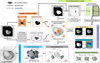 |
Fig. 1 Framework of Asteroid-GS. The input to the framework is multi-view images captured by the spacecraft. We initialize the 3D Gaussian scene using the sparse point cloud generated by SfM. We dilate the masks segmented from SAM alongside statistical filtering to achieve adaptive Gaussian pruning. The MLPs integrated with illumination information are employed to predict the colors of 3D Gaussian primitives in well-lit and shadowed areas. Geometric regularization techniques are introduced to enhance the accuracy and robustness of reconstruction. We construct the Gaussian opacity field and identify the level set before extracting the surface mesh. |
3.3 Adaptive Gaussian pruning
As presented in Fig. 2, we utilized the visual cones from morphologically dilated masks to derive the external shape of asteroid, effectively removing noise around the surface model. Additionally, to optimize the internal shape of asteroid, we employed a statistical filtering method to prune primitives with extreme scales or highly dispersed positions, refining the density of 3D Gaussian primitives.
3.3.1 Gaussian pruning strategy based on dilated masks
During the densification of the 3DGS, 3D Gaussian primitives undergo splitting and cloning, while those with low opacity are pruned. However, this straightforward approach is not sufficient to remove noisy primitives around the asteroid. To address this, we first utilized SAM to generate a segmentation mask of the asteroid:
 (5)
(5)
where  is the l-th input red-green-blue image, ESAM is the estimator of SAM, and
  is the output segmentation mask. Foreground pixels are assigned a value of 1, while those in the background are set to 0. After that, we projected the centers of the 3D Gaussian primitives from the world space onto the image plane as follows:
 (6)
(6)
where μk = (xk, yk, zk)⊤ is the center of the k-th 3D Gaussian primitive in the scene, pk = (uk, vk)⊤ is the corresponding projected coordinate on the image. If pk is within the foreground of the segmentation mask  , it is retained; otherwise, it is discarded. In this manner, we ensured that all 3D Gaussian primitives are confined within the visual hull, defined by the intersection of visual cones from different segmentation masks, effectively eliminating background noise throughout the training process:
 (7)
(7)
where L is the number of all viewpoints and μ′k denotes the remaining 3D Gaussian primitives. However, since the segmentation mask output by SAM is at the pixel level, it is difficult to identify shadowed areas. Additionally, each 3D Gaussian primitive has a coverage radius in its projection, allowing a single primitive to affect multiple pixels from a single viewpoint. Therefore, directly using the segmentation mask output by SAM for pruning would lead to the incorrect removal of valid 3D Gaussian primitives. To preserve those valid ones, we employed a morphological dilation technique to expand the segmentation masks, ensuring a more inclusive foreground representation, as follows:
 (8)
(8)
where S is the structuring element, t is the pixel coordinate on the image, ⊕ represents dilation operation, (S)t denotes translating the structuring element S to coordinate t, and  is the dilated mask, which is a binary image. Then, we used
  to replace
  in Eq. (7) for pruning.
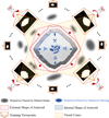 |
Fig. 2 Illustration of the adaptive Gaussian pruning strategy. The intersection of all visual cones from different viewpoints contributes to define the external shape of the asteroid by eliminating the 3D Gaussian primitives outside the dilated masks. Statistical filtering facilitates the refinement of the internal shape by removing discrete primitives within the asteroid. |
3.3.2 Adaptive densification based on statistical filtering
The naïve 3DGS prunes 3D Gaussian primitives with large scales and extensive coverage during the densification process. However, it relies on fixed thresholds and lacks the flexibility to effectively remove poorly fitting primitives. To address this, we applied a statistical filtering method to adaptively prune primitives with unsuitable scales and excessive dispersion. Assuming there are K primitives in the 3D Gaussian scene, we calculated the mean and variance of their scales. The scale s̄k is defined as the average size sk along the x, y, z axes for each 3D Gaussian primitive:
 (9)
(9)
 (10)
(10)
where X̄s and  are the sample mean and variance of the scales of the 3D Gaussian primitives. For each primitive, it is retained if τmin < s̄k < Tmax; otherwise, it is discarded. The values of τmin and τmax are computed as follows:
 (11)
(11)
where λs is the adjustable coefficient for the sample variance of scales, τmin and τmax can be viewed as the upper and lower limits. Likewise, we performed statistical filtering on the positions of the 3D Gaussian primitives. First, we defined a neighborhood for each primitive and assign the nearest H primitives to it. Then, we computed the average distance from this primitive to other primitives in the neighborhood:
 (12)
(12)
where dkh is the distance from the k-th 3D Gaussian primitive to the h-th primitive in its neighborhood, dk is introduced as a new attribute for the k-th primitive. Next, we computed the mean and variance of the distances among the K primitives, along with the thresholds γmin and γmax:
 (13)
(13)
 (14)
(14)
where X̄d and  are the sample mean and variance of the distances, λd is the adjustable coefficient, γmin and γmax are adaptive thresholds. For each 3D Gaussian primitive, if its distance attribute satisfies γmin < dk < γmax, it is retained; otherwise, it is pruned. This enables the removal of primitives with excessively dispersed positions, thereby refining their density within the asteroid.
3.4 Asteroid illumination learning
To better model the complex illumination on the asteroid surface, we used the MLPs shown in Fig. 3 to regress the colors of 3D Gaussian primitives. This module consists of MLPlight and MLPshadow, which respectively predict the colors of primitives in well-lit and shadowed regions. We combined the segmentation masks from SAM and the α-blending masks from the 3D Gaussian scene to label primitives in two different regions. Furthermore, we integrated additional illumination information, including the angle between the primitive and the incident light, as well as the camera position related to the asteroid’s spin, to enhance the performance of MLPs.
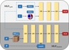 |
Fig. 3 MLPs integrated with illumination information. They are composed of two parts: MLPlight and MLPshadow. In well-lit regions on the asteroid surface, MLPlight takes as input the positional encoded (PE) camera centers (o) and SH coefficients (c) of 3D Gaussian primitives to regress the red-green-blue colors. In shadowed regions, MLPshadow additionally incorporates the hash-encoded (HE) mean (μ) of 3D Gaussian primitives and the angle (θ) between each primitive and the incident light to perform the regression of red-green-blue colors. |
3.4.1 Well-lit and shadowed region identifications
Due to the occlusion caused by the irregular shape of the asteroid, parallel incident sunlight casts shadows on its surface. The light intensity of shadowed regions fluctuates periodically due to the asteroid’s spin, often leading to errors in surface reconstruction. Accurately identifying and separately processing the shadows can enhance the performance of 3DGS. The technical workflow for shadow identification is presented at the top of Fig. 1. Firstly, we utilized SAM to generate pixel-level segmentation masks, as expressed in Eq. (5). Since there is no prior knowledge of the asteroid’s shape, SAM’s segmentation masks exclude shadowed regions, capturing only well-illuminated areas. Then, the 3D Gaussian scene produces the α-blending masks  as follows:
 (15)
(15)
 (16)
(16)
Since the 3D Gaussian scene has learned the asteroid’s approximate shape after preparatory training with adaptive Gaussian pruning, the α-blending mask can be regarded as an instancelevel mask. By performing a bitwise operation on  and
and  , the shadowed regions
  can be identified:
 (17)
(17)
where l is the index of the image,  is the inverse of
  . We assigned distinct labels to the 3D Gaussian primitives projected into well-lit or shadowed regions and used the MLPs introduced later to regress their colors.
3.4.2 MLPs integrated with illumination information
The surface of an asteroid is often covered with regolith, a loose layer of fragmented material formed by micrometeorite impacts and space weathering. Although the surface characteristics differ among various asteroid types (C-type, S-type, and M-type), their reflection properties can be approximated using the Lambertian reflection model (Lambert 1760) as follows:
 (18)
(18)
where Ir represents the intensity of the reflected light, Ii denotes the intensity of the incident light, m corresponds to the diffuse reflection coefficient of the surface material, while Ii and n respectively indicate the directions of the incident light and the surface normal. To simplify this model, we assumed that the incident light intensity and the surface diffuse reflection coefficient remain constant for a given asteroid. In contrast, the angle between the surface normal and the incident light varies with the asteroid’s shape, resulting in changes in reflected light intensity. We treated the direction of the line connecting the 3D Gaussian primitive to the center of the 3D Gaussian scene as the asteroid’s surface normal, then used it to compute the varied angle θk before inputting the cos θk to the MLPshadow:
 (19)
(19)
 (20)
(20)
where pc is the center of the 3D Gaussian scene, ps is the position of the Sun. cos θk acts as an approximate substitute for cos(Ii, n).
The asteroid’s surface is periodically illuminated by sunlight due to its spin, leading to cyclical variations in brightness. Given the relative motion between the asteroid and the spacecraft, the asteroid’s spin is equivalent to the spacecraft orbiting around the asteroid. We employed SfM to estimate the extrinsic parameters of the cameras, incorporating their center positions as a supplementary input to the MLPlight and MLPshadow. As high-frequency input is more beneficial to the MLPs, we applied positional encoding (PE; Rahaman et al. 2019) to the camera centers:
 (21)
(21)
where p ∈ R is the scalar component of the coordinate of the camera center o ∈ R3. This process means mapping a lowerdimensional space R into a higher-dimensional space R2n.
To accelerate training, we performed hash encoding of multiresolution voxel grids (Müller et al. 2022) for the 3D Gaussian primitives and input them to MLPshadow. We identified the voxels surrounding the primitives and use the feature vectors to trilin-early interpolate the mean μk of each primitive. Then, the hash codes h(μk,r) at different resolutions are concatenated:
 (22)
(22)
where l represents the level of the multi-resolution grid. Meanwhile, to enhance color representation, the SH coefficients of each 3D Gaussian primitive are preserved and fed into both the MLPlight and MLPshadow, optimized alongside the hash features during the training process.
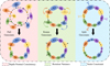 |
Fig. 4 Illustration of geometric regularization techniques. To ensure compact representation, the depth-normal consistency loss pulls the 3D Gaussian primitives to the asteroid surface. The rotation variance loss rotates the 3D Gaussian primitives to avoid identical orientations, improving the fit to the elliptical shape of asteroids. The scale constraint loss splits oversized 3D Gaussian primitives to better capture fine details. |
3.5 Geometric regularization
To improve the geometric accuracy, we introduced the depthnormal consistency loss to pull the 3D Gaussian primitives closer to the object surface, as shown in Fig. 4. Moreover, to enhance the robustness and capture of details, we introduced a rotation variance and scale constraint loss to rotate and split 3D Gaussian primitives, preventing uniformly oriented and excessively large primitives from causing the training to converge to local minima.
3.5.1 Depth-normal consistency loss
Relying solely on photometric loss in the naïve 3DGS results in a less compact distribution of 3D Gaussian primitives, making it difficult to achieve high-quality surface reconstruction. To address this, we incorporated the depth-normal consistency loss (Ln) from 2DGS (Huang et al. 2024), ensuring the alignment of 3D Gaussian primitives with the asteroid surface:
 (23)
(23)
where i indexes intersected 3D Gaussian primitives along the ray, with  representing the blending weight of the primitive. The normal of the i-th primitive is denoted as ni, while ñ corresponds to the surface normal direction obtained via finite difference applied to the depth map. Specifically, the depth maps are generated through a rasterization-based approach (Zhang et al. 2024).
3.5.2 Rotation variance loss
The gravity of asteroids redistributes surface material, typically shaping them into a sphere or an ellipsoid. Considering the prior knowledge of the asteroid’s shape, we argue that the rotations of 3D Gaussian primitives should be varied rather than uniformly oriented. To be specific, the rotation attribute qk of 3D Gaussian primitives for asteroid should not be completely identical, as this could lead the model to fall into a suboptimal result. We employed the rotation variance loss to avoid this:
 (24)
(24)
where k means the k-th 3D Gaussian primitive, while j represents the j-th component of the quaternion qk. When the rotations of 3D Gaussian primitives are identical, the variance of qjk approaches zero, leading to an increase in the loss Lr, which penalizes overfitted primitives with the same orientations.
3.5.3 Scale constraint loss
The asteroid surface is typically covered with weakly textured regolith, making it challenging to capture small-scale features. Especially when oversized primitives exist in the 3D Gaussian scene, it is more likely to result in missing of fine details. To alleviate this, we regulated the scales of the 3D Gaussian primitives by applying the scale constraint loss:
 (25)
(25)
where  , indicating that the scale of the 3D Gaussian primitive is determined by the maximum size along the x, y, z axes. Since most primitives in the 3D Gaussian scene are relatively small in our experiments, the presence of oversized primitives will increase the loss Ls, thereby penalizing those under-fitted primitives with excessively large scales.
3.5.4 Total loss
Finally, we aggregated the above loss functions to enhance geometric regularization in asteroid surface reconstruction:
 (26)
(26)
where Lc denotes the photometric loss in the naïve 3DGS, Ln stands for the depth-normal consistency loss, Lr is the rotation variance loss, and Ls is the scale constraint loss. The coefficients ωc, ωn, ωr, and ωs are the weights of the corresponding loss functions.
3.6 Surface mesh extraction
In conventional surface extraction methods, Poisson reconstruction ignores the scales of primitives and is susceptible to noise, while TSDF fusion tends to produce missing regions at the poles of the asteroid model due to insufficient viewpoints. To extract high-precision asteroid model, we constructed the continuous Gaussian opacity field based on a ray-sampling volume rendering method (Yu et al. 2024c).
First, we utilized the 3D covariance matrix Σ3D to transform the world coordinate system to the local coordinate system for each 3D Gaussian primitive and normalize the scale. Within the local coordinate system, the 3D Gaussian along the ray is simplified to a 1D Gaussian:
 (27)
(27)
The 3D point xg is computed by transformed camera center og and ray direction rg through xg = og + trg. For a 1D Gaussian, the maximum value can be determined using a closed-form solution  . The opacity along the ray increases monotonically until it reaches its maximum value G1 d(t*), after which it stays constant. Consequently, the accumulated opacity can be computed via volume rendering:
 (28)
(28)
Since a 3D point x might be visible from multiple training views, its opacity is defined as the minimum opacity value observed across all training views and observation directions. The opacity of any point can be calculated in this way.
To incorporate the scales of primitives into surface reconstruction, we generated a 3D bounding box with the side length of 3 sk centered at each 3D Gaussian primitive. Then, we evaluated the opacity of points at both the center and the vertices of these bounding boxes. However, this could introduce some noise points in our experiment. To remove the noise points, we utilized the dilated masks to filter out unreliable ones. To accelerate computation, we conducted a binary search to identify the level set where the opacity reaches 0.5. Finally, we used the marching tetrahedra algorithm to extract the surface mesh.
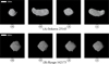 |
Fig. 5 Examples of images used for surface reconstruction of Itokawa (A) and Ryugu (B). The white lines represent the proportional relationship between the actual distance in space and the corresponding distance in the images. |
4 Experiments and discussion
In this section we evaluate our proposed framework on two real asteroid datasets—Itokawa (25143) and Ryugu (162173)—to demonstrate its effectiveness. As this study focuses on intelligent and fast 3D reconstruction from limited data, we compare our method with state-of-the-art (SOTA) 3DGS-based approaches to highlight its advantages, and with the classical SPG and SPC methods to demonstrate its comparable accuracy to traditional techniques. Furthermore, we conduct ablation studies to validate the contribution of each module within the proposed framework.
4.1 Datasets of asteroids
The Japan Aerospace Exploration Agency (JAXA) launched the Hayabusa spacecraft on May 9, 2003, to explore the near-Earth asteroid Itokawa (25143) and return surface samples (Fujiwara et al. 2006). The Asteroid Multiband Imaging Camera (AMICA) was a narrow-angle camera on board the Hayabusa, designed to capture high-resolution images of Itokawa. AMICA recorded approximately 1400 images during the spacecraft’s rendezvous phase with Itokawa, at a spatial resolution ranging from 0.3 to 0.8 meters. This paper selected 60 images taken between September 28 and October 2, 2005, at a distance of 7-8 km from the asteroid for the experiment. Among them, 10 images were randomly assigned to the test set, while the remaining 50 images were used as the training set to reconstruct the asteroid. Itokawa’s ellipsoidal shape resembles that of a sea otter, consisting of a “head” and a “body,” with the region between them referred to as the “neck,” as shown in Fig. 5A. The images captured from the equator offer an even distribution of viewing angles across the surface of Itokawa, as shown in Fig. 6A. The camera poses are estimated using the SfM method. The coordinate system is based on the Itokawa body-fixed frame, consistent with the SPC model provided by Gaskell et al. (2008). The basic information of the Itokawa dataset is provided in the second column of Table 1, and example images with a resolution of 1024 × 1024 pixels are shown in Fig. 5A.
Ryugu (162173) is another near-Earth asteroid, observed by the Hayabusa2 spacecraft, which visited Ryugu in 2018 and returned in 2020 with surface samples (Watanabe et al. 2019a). The Optical Navigation Camera Telescope (ONC-T) onboard the spacecraft was used to capture high-resolution images of Ryugu. This paper uses 60 images taken between 6:05 AM and 1:55 PM on July 10, 2018, for reconstruction. Similarly, the dataset is divided into a training set and a test set in a 5: 1 ratio. These images were captured by the spacecraft from the equatorial plane of Ryugu at a distance of 20-21 km, providing comprehensive coverage of the asteroid’s surface, as shown in Fig. 5B and Fig. 6B. The geological characteristics of Ryugu are primarily defined by a high density of impact craters and a low-cohesion regolith layer. Ryugu has a shape that is more spherical, while Itokawa has a more elongated shape. The coordinate system corresponds to that of the SfM+MVS model from Watanabe et al. (2019a). The third column of Table 1 presents the basic information of the Ryugu dataset, and Fig. 5B displays example images with a resolution of 1024 × 1024 pixels.
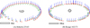 |
Fig. 6 Camera poses for the selected images used in surface reconstruction for Itokawa (A) and Ryugu (B). The rectangles with black outlines represent the proportional relationship between the actual distance in space and the corresponding distance on the maps. |
Basic information of the Itokawa and Ryugu datasets.
4.2 Evaluation criteria
To directly assess the quality of reconstruction among different methods, we evaluated the similarity between the reconstructed model and the reference model. Specifically, we computed the histogram of the distance map between two 3D models. Then we calculated the mean distance (mean), root mean square error (RMSE), and standard deviation (Std.Dev.) as evaluation metrics. Let G1 and G2 represent two 3D models, with point sets P1 = {p1, p2, p3,...} and P2 = {q1, q2, q3,...}, where each point pi and qi is a coordinate in the 3D space (pi, qi ∈ R3).
The mean distance is the average distance between corresponding points of two 3D models, reflecting their overall shape difference. The formula for mean distance is
 (29)
(29)
where pi is the i-th point in the mesh G1, and qi is the point in mesh G2 that is closest to pi. The nearest-point search can be conducted using either a linear search or nearest-neighbor matching. ∥·∥ denotes the Euclidean distance between pi and qi. n represents the number of sampling points. Notably, this is an undirected distance, meaning that distances in opposite directions do not neutralize each other.
The RMSE is the square root of the average squared distance between corresponding points of two models. It is more sensitive to areas with significant deformation or mismatch:
 (30)
(30)
The Std.Dev. measures the dispersion of distances between corresponding points in two 3D models, reflecting how the distances vary around the mean:
 (31)
(31)
Lower mean, RMS, and Std.Dev. values indicate smaller differences between the two 3D models, reflecting higher shape similarity between the reconstructed model and the reference model.
In addition, 3DGS-based methods can be applied not only to 3D reconstruction but also to NVS. Therefore, when comparing with the SOTA 3DGS-based methods, we indirectly assessed the quality of reconstruction by evaluating the similarity metrics of NVS. Specifically, we input the camera poses from the test set, render images using the 3DGS-based method, and compared them with the ground truth images for similarity. We chose three widely used image similarity metrics for assessment: the peak signal-to-noise ratio (PSNR), the structural similarity index (SSIM), and the learned perceptual image patch similarity (LPIPS).
The PSNR is a pixel-based metric used to evaluate the quality of image reconstruction. It is computed from the mean squared error (MSE) between the rendered image and the ground truth, representing the ratio of the maximum signal to the error. The formula for PSNR is
 (32)
(32)
where Imax is the maximum intensity of the images (255 for 8-bit images), Ia and Ib represent the grayscale values corresponding to image a and image b.
The SSIM focuses on perceptual image quality, as human perception is influenced not only by pixel differences but also by factors such as brightness, contrast, and structure. A value of SSIM closer to 1 indicates a higher structural similarity between the two images:
 (33)
(33)
where μa and μb are the mean values (brightness) of images a and b,  and
and  are the variance values (contrast), σab is the covariance between the two images (structure). The constants C1 = (K1 Imax)2 and C2 = (K2Imax)2 are typically set to K1 = 0.01 and K2 = 0.03.
The LPIPS is a deep learning based image similarity metric. Unlike PSNR and SSIM, LPIPS does not rely on pixel-level differences or statistical characteristics. Instead, it computes perceptual similarity by using high-level features extracted from a deep neural network φ. LPIPS argues that perceptual differences provide a more accurate representation of human subjective experience than simple pixel-wise differences:
 (34)
(34)
where φl represents the feature map output by the l-th layer of the pretrained neural network, Hl and Wl represent the height and width of the feature map at the l-th layer. Higher values of both PSNR and SSIM indicate greater image similarity, while lower LPIPS values correspond to higher similarity.
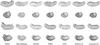 |
Fig. 7 Comparison of the reconstruction results from the Asteroid-GS method and SOTA 3DGS-based methods for asteroid Itokawa (25143). |
4.3 Implementation details and baselines
All experiments were conducted on an Ubuntu 20.04 system, implemented using Python 3.9.21 and PyTorch 2.0.0. The hardware environment consisted of an Intel i7-6850 K @ 3.60 GHz processor and an NVIDIA RTX 3090 GPU. The Adam optimizer was used for gradient-based optimization. Training was performed for a total of 30000 iterations. The rotation variance and scale constraint loss were introduced after 7000 iterations, followed by the depth-normal consistency loss at 15,000 iterations. The structuring element S was defined as a circular shape with a radius of 40 pixels. The adjustable coefficients for statistical filtering, λs and λd, were set to 100 and 1000, respectively. The dimensionality of the high-dimensional vector in position encoding was set to 4, while the hierarchical level of the hash grid resolution was set to 2. The corresponding weights for the loss components in the total loss were set to ωc = 1, ωn = 0.05, ωs = 100, and ωr = 10. To comprehensively evaluate the effectiveness of the proposed method, we conducted comparative experiments on NVS and 3D model differences against SOTA 3DGS-based methods, including 3DGS, mip-splatting, SuGaR, 2DGS, GOF, and RaDe-GS.
4.4 Results: Itokawa
4.4.1 Comparison with 3DGS-based methods
We compared the proposed Asteroid-GS with several SOTA 3DGS-based methods. It can be seen that Asteroid-GS surpasses all SOTA methods in all metrics. This is clearly demonstrated by the 3D maps of the shape models, as shown in Fig. 7. The models reconstructed using other 3DGS-based methods exhibit noticeable geometric noise and surface defects, whereas the Asteroid-GS results are more complete and refined. The naïve 3DGS model displays significant geometric distortion, making it difficult to identify the asteroid’s surface features, particularly in the polar regions. The mip-splatting model lacks surface regularization constraints, leading to discontinuous and fragmented surfaces. The SuGaR model is relatively complete but lacks texture and finer details. The 2DGS model has a low surface mesh resolution, resulting in noticeable mosaic artifacts. The GOF model also exhibits surface defects, with holes appearing in certain local regions. The surface of the RaDe-GS model displays irregular protrusions in shadowed regions. In contrast, the Asteroid-GS model features a seamless and continuous surface, exhibiting fine surface details and high geometric accuracy. Even in the polar regions, it reconstructs a correct result, as shown in Fig. 8A. The metrics for the comparative results are presented in Table 2. Our method achieves the best results in both NVS metrics and 3D reconstruction metrics. The NVS metrics are computed on the test set, with a PSNR of 43.6945, an SSIM of 0.9945, and an LPIPS of 0.0112. The mean distance, RMSE, and Std.Dev. are calculated using the high-precision Itokawa model of Gaskell et al. (2008) as the reference model, which is commonly used in other methods (Chen et al. 2024a,b). As indicated in Table 2, our method is the only one achieving a reconstruction error within 1 meter.
Comparison of SOTA 3DGS-based methods for the Itokawa (25143) dataset.
4.4.2 Comparison with traditional methods
To validate the consistency of our method with the traditional method, we computed the distance map from our Asteroid-GS model to the reference model, as shown in Fig. 9A. The reference model was reconstructed using 775 images with the SPC method, as shown in Fig. 8C, significantly surpassing our 50 input images. In addition, we used the same set of 50 images as input and employed photogrammetry software to generate the SPG model, as shown in Fig. 8B. Then we computed distance map between the SPG model and the reference model, as shown in Fig. 9B. The quantitative comparison between the reconstructed models and the reference model, as shown in Table 4, demonstrates that our model closely approximates the reference model, with a mean of 0.7053 m, RMSE of 0.9627 m, and Std. Dev. of 0.9613 m. Our method can achieve this accuracy in less than 40 minutes, taking significantly less computation time than the SPC (Weirich et al. 2022) and NeRF-based methods (Chen et al. 2024a,b). Our method is competitive compared with existing NeRF-based methods, where Chen et al. (2024a) achieved an RMSE of 1.196 m using 52 images, requiring approximately 2-3 days of computation, while Chen et al. (2024b) reconstructed Itokawa with a Std. Dev. of 0.858 m using 172 images in 7.7 hours. Moreover, our method outperforms the SPG method, particularly in the polar regions, where the SPG method exhibits significant errors. As shown in Fig. 9a, b, and c, the SPG model exhibits incorrect protrusions. These discrepancies may stem from the lack of polar viewpoints when observing the asteroid. In contrast, our method maintains good reconstruction results globally, with the histogram in Fig. 9 showing a more concentrated distribution around the mean. In some local regions, such as areas in Fig. 9d, our method captures even the details that the reference model overlooks. Despite some blue regions remaining in the distance maps between our model and the reference model, as shown in Fig. 9e, our method achieves smaller reconstruction errors compared to the SPG method. As shown in Fig. 8, our shape model exhibits geometric consistency with traditional models. We calculated the volume, surface area, and average edge length of our model, as well as those of the SPG and SPC shape models, as summarized in Table 5. The volume can be used to estimate the asteroid’s density, thereby indirectly validating the model’s reliability (Gaskell et al. 2008; Watanabe et al. 2019a,b), while the average edge length serves as an indicator of the geometric resolution of the model (Chen et al. 2024b). Compared with the SPG model, our shape model exhibits closer agreement with the high-resolution SPC model in terms of volume, surface area, and mean edge length. Specifically, the volume of our shape model is estimated to be 0.01769 km3, which is closer to the SPC model volume of 0.01773 km3 than the SPG model volume of 0.01654 km3. The average edge length of our model is smaller than that of the SPG model, suggesting that it captures finer geometric details. Since the SPC model incorporates a substantially larger number of images and LIDAR (Light Detection And Ranging) data for constraint and joint solutions, it achieves the smallest average edge length among the three models.
4.5 Results: Ryugu
4.5.1 Comparison with 3DGS-based methods
We utilized the high-precision model of Ryugu from Watanabe et al. (2019a) as the reference model for the comparative experiment. We compared our method with SOTA 3DGS-based approaches, as shown in the quantitative metrics in Table 3, where our method achieves the best results across all evaluated metrics. Asteroid-GS achieves the highest NVS metrics, with a PSNR of 41.7110, an SSIM of 0.9902, and an LPIPS of 0.0165, demonstrating that our method produces the most accurate and visually consistent renderings. As illustrated in the 3D maps of the shape models in Fig. 10, the model of Asteroid-GS clearly surpasses those produced by other methods. The naïve 3DGS model is almost submerged in noise. The mip-splatting model appears to be composed of discrete point clouds. The surface of the SuGaR model is overly smooth and the 2DGS model has degraded contour details. The GOF model exhibits numerous holes on its surface. The RaDe-GS model fails to capture the structural features of the boulders in the polar regions. In contrast, the Asteroid-GS model features high-resolution surface details while maintaining both surface integrity and continuity. More reconstruction results of the Asteroid-GS are shown in Fig. 11A.
4.5.2 Comparison with traditional methods
To compare the shape accuracy of our model with the SPG model, we respectively computed the distance maps from the Asteroid-GS model and the SPG model to the reference model, as shown in Figs. 12A and B. The reference model was generated using 214 images, nearly four times our input of 50 images.
Similar to the previous case, the SPG model is reconstructed with the same set of 50 images as input. The 3D reconstruction metrics are presented in Table 7, demonstrating that our model is structurally consistent with the reference model. Furthermore, our model outperforms the SPG model, with a mean of 1.3411 m, RMSE of 1.9058 m, and Std.Dev. of 1.9036 m, which can also be clearly seen in Fig. 11A. Our method reconstructs asteroid Ryugu in under 40 minutes, similar to the reconstruction time for Itokawa mentioned earlier. Compared to the SPG model, our model captures more delicate details. As illustrated in the histograms in Fig. 12, the Asteroid-GS method exhibits a narrower error distribution range compared to the SPG method, indicating that the reconstruction error between the AsteroidGS model and the reference model is smaller than that of the SPG model. As shown in Fig. 11, the surface mesh of the SPG model exhibits mosaic artifacts and sharp edges, while our Asteroid-GS model features a smoother and more detailed reconstruction. To comprehensively evaluate our shape model, we also visualized the Ryugu asteroid model reconstructed via the SPC method (Watanabe et al. 2019b), as shown in Fig. 11C. A total of 1217 ONC-T images were used to reconstruct this SPC model. The Std.Dev. of the height differences between the SPC model (Watanabe et al. 2019b) and the SfM model (Watanabe et al. 2019a) is approximately 1.5 m. Compared with the SPG shape model, our model shows greater similarity to the high-resolution SPC model of asteroid Ryugu. In particular, in the polar regions, our method successfully reconstructs the geometry using only equatorial imaging data. The SPG method typically relies on additional hole-filling algorithms to generate a complete model, yet it still exhibits certain limitations in capturing fine-grained polar surface features, as shown for the + Z and -Z regions in Fig. 11B. The quantitative results in Table 6 further demonstrate that the volume, surface area, and average edge length of our model are more consistent with those of the SPC model. The estimated volume of our shape model is 0.37658 km3, which closely matches the SPC-derived model volume of 0.37952 km3. Meanwhile, our model’s average edge length is 1.861 m, significantly finer than the 2.641 m of the SPG model and closer to the 1.473 m achieved by the SPC model.
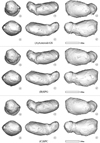 |
Fig. 8 Overviews of the reconstructed asteroid Itokawa (25143) using our Asteroid-GS method, the SPG method, and the SPC method. The subscripts of 3D maps represent different viewing directions. |
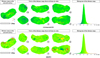 |
Fig. 9 Visualization of distance maps relative to the reference model for our Asteroid-GS method and the SPG method on asteroid Itokawa (25143). Views observed from six directions (+x, -x, +y, -y, + z, -z) comprehensively highlight the differences. The histograms of the distance maps on the right illustrate the statistical distribution of distances. Compared to the SPG method, which exhibits a broader distribution with deviations up to nearly 10 meters, our proposed Asteroid-GS method achieves a more concentrated distribution within 5 meters. |
Comparison with SOTA 3DGS-based methods for the Ryugu (162173) dataset.
Statistical results of the distance maps based on the reference model of the asteroid Itokawa (25143).
Comparison of geometric parameters of the shape models of asteroid Itokawa (25143).
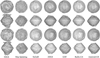 |
Fig. 10 Comparison of reconstruction results from the Asteroid-GS method and SOTA 3DGS-based methods for asteroid Ryugu (162173). |
4.6 Ablation studies
In this section we validate the effectiveness of various modules in our method, including adaptive Gaussian pruning strategy, asteroid illumination learning, geometric regularization and surface mesh extraction method. We compare the experimental results obtained before and after disabling each module to assess their impact. The specific quantitative metrics are presented in Table 8.
All metrics decline when the adaptive Gaussian pruning strategy is removed. This is because the absence of the pruning strategy causes the small asteroid model to be overwhelmed by noise. The asteroid illumination learning includes two modules: the MLPs and shadow recognition. Omitting either of these modules leads to a decline in the metrics, indicating that illumination learning is crucial for asteroid surface reconstruction. When geometric regularization is disabled, the reconstruction accuracy also decreases. Moreover, computing the Gaussian opacity field helps enhance 3D reconstruction metrics by generating a more continuous surface, while the metrics for NVS remain unchanged since the surface mesh extraction is not involved in the training process of the 3DGS.
4.6.1 Effects of the adaptive Gaussian pruning strategy
As shown in Fig. 13, the absence of the adaptive Gaussian pruning strategy leads to the appearance of redundant facets around the asteroid model. These facets are generated from unnecessary 3D Gaussian primitives, which are introduced due to noise interference in the deep space environment. The positions of these noise facets during each training process are random and, in severe cases, can completely overwhelm the entire asteroid model, significantly degrading the reconstruction quality. However, once the pruning strategy is applied, the redundant facets around the asteroid are effectively eliminated. In fact, the adaptive Gaussian pruning strategy constructs a visual hull for the 3D Gaussian scene, defined by the intersection of all visual cones from different viewpoints. This ensures that the reconstruction focuses on the surface of the asteroid rather than the entire deep space environment.
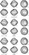 |
Fig. 11 Overviews of the reconstructed asteroid Ryugu (162173) using our Asteroid-GS method, the SPG method, and the SPC method. The subscripts of 3D maps represent different viewing directions. |
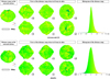 |
Fig. 12 Visualization of distance maps relative to the reference model for our Asteroid-GS method and the SPG method on asteroid Ryugu (162173). Views observed from six directions (+x, -x, +y, -y, + z, -z) comprehensively highlight the differences. The histograms of the distance maps on the right illustrate the statistical distribution of distances. The SPG method exhibits more distances distributed away from the histogram center, indicating that many regions have significant errors. In contrast, our Asteroid-GS method shows a narrower range in the histogram, suggesting higher reconstruction accuracy. |
Comparison of geometric parameters of the shape models of asteroid Ryugu (162173).
4.6.2 Effects of asteroid illumination learning
Based on the results presented in Figs. 14 and 15, the impact of illumination learning on the reconstruction of the asteroid’s surface is distinctly evident. Without the MLPs regressing the color of 3D Gaussian primitives, the asteroid’s surface geometry suffers from significant defects. As illustrated in Fig. 14, disabling the MLPs with illumination information leads to noticeable depressions on the asteroid’s surface. This causes the asteroid’s surface to experience an inward displacement in areas with poor lighting. Since the light intensity on the asteroid’s surface fluctuates periodically with its spin, it is insufficient to calculate the colors of 3D Gaussian primitives using only SH coefficients. After applying the MLPs, the 3DGS more effectively captures the variations in lighting on the asteroid’s surface, thereby significantly improving the accuracy of surface reconstruction. Furthermore, as shown in Fig. 15, disabling the shadow recognition module results in irregular protrusions on the surface shadowed areas. This suggests that the 3D Gaussian representation failed to learn the shadowed areas during training, mistakenly treating the shadows caused by occlusion as black terrain on the asteroid’s surface. After applying our method to identify shadows and utilizing the MLPs to process the shadow regions, the erroneous protrusions on the asteroid’s surface are effectively removed. The results in Table 8 demonstrate that both the MLPs and shadow recognition contribute to improving the performance of NVS and the quality of the 3D model.
Statistical results of the distance maps based on the reference model of the asteroid Ryugu (162173).
Ablation study results on the Itokawa (25143) and Ryugu (162173) datasets.
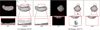 |
Fig. 13 Ablation study of adaptive Gaussian pruning for asteroid Itokawa (25143) and Ryugu (162173). A large number of redundant facets appear around the asteroid surface model, caused by noise interference in deep space. The noise is eliminated after adaptive Gaussian pruning. |
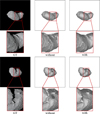 |
Fig. 14 Ablation study of MLPs. Without the use of the MLPs, incorrect surface shapes appear on the asteroid. |
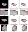 |
Fig. 15 Ablation study of shadow recognition. The absence of shadow recognition leads to irregular protrusions on the asteroid surface. |
4.6.3 Effects of regularization improvement
The introduced geometric regularization refines the details of the asteroid’s surface, improving the accuracy of surface reconstruction. To observe the changes in the 3D Gaussian primitives with and without the regularization, we rendered the normal maps of asteroid surface as presented in Fig. 16. We used pseudo-colors to visually represent the ellipsoid-shaped 3D Gaussian primitives. When geometric regularization is not applied, oversized 3D Gaussian primitives appear across the asteroid’s surface. 3D Gaussian primitives with too large scales or uniform orientations can cause over-smoothing, resulting in the loss of fine details. Adding geometric regularization enables the 3D Gaussian primitives to better conform to the asteroid’s surface and accurately capture fine-scale features.
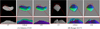 |
Fig. 16 Ablation study of geometric regularization for asteroid Itokawa (25143) and Ryugu (162173). The pseudo-color images represent the normal maps rendered from the 3D Gaussian scene. Without geometric regularization, 3D Gaussian primitives are difficult to fit the asteroid surface. |
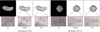 |
Fig. 17 Ablation study of the Gaussian opacity field for asteroid Itokawa (25143) and Ryugu (162173). We compare surface models extracted using TSDF fusion and our method. Extraction from the Gaussian opacity field facilitates obtaining a more detailed asteroid surface model. |
4.6.4 Effects of the surface mesh extraction method
Surface mesh extraction involves computing the Gaussian opacity field to identify the level set and employing the marching tetrahedra algorithm to generate the final 3D model. Other 3DGS-based methods often use TSDF fusion to extract surface meshes. Figure 17 illustrates the effectiveness of our module. We applied our surface mesh extraction method to the Itokawa and Ryugu datasets and compared the results with those obtained through TSDF fusion. The 3D model generated by TSDF fusion lacks surface details and has blurred textures. In contrast, our method produces a more refined 3D model, successfully capturing even small rocks on the asteroid’s surface. Furthermore, due to the limited viewpoint coverage in polar regions, TSDF fusion often results in incomplete reconstructions. Instead, computing the Gaussian opacity field helps achieve a more complete asteroid model.
5 Conclusions
In this work we present Asteroid-GS, a novel framework based on 3DGS for intelligent asteroid surface reconstruction. Our approach enables the fast generation of high-fidelity 3D models from a limited set of input images. We developed an adaptive Gaussian pruning strategy to effectively mitigate noise in deep space. With the employment of MLPs integrated with illumination information, we improve the modeling of illumination on the asteroid surface. Furthermore, the geometric regularization and efficient surface mesh extraction enhance the accuracy of the reconstruction. The experimental results show that our method outperforms SOTA 3DGS-based methods in asteroid surface reconstruction. Compared to NeRF-based methods, our method achieves substantially faster performance. Moreover, our automated method significantly reduces the need for manual intervention while maintaining shape consistency with the traditional SPC method. With the same number of input images, our method surpasses the SPG method. Overall, Asteroid-GS represents a significant advancement in fast and intelligent asteroid surface reconstruction, enriching the toolkit for asteroid surface reconstruction.
Regarding future work, we aim to further reduce the data requirements of our reconstruction method even in cases with just a few images, which are likely to be encountered in actual asteroid exploration missions. With the upcoming Tianwen-2 exploration mission, we plan to test our method on the returning data from asteroid 2016 HO3 and comet 311P.
Acknowledgements
This work was supported by the key Laboratory of Spaceflight Dynamics Technology Foundation under grant number ZBS-2023-004. The authors gratefully acknowledge the efforts of those who facilitated the archiving and open dissemination of images and datasets related to the asteroids Itokawa and Ryugu, which have been invaluable to this research.
References
- Chapman, C. R., & Morrison, D. 1994, Nature, 367, 33 [NASA ADS] [CrossRef] [Google Scholar]
- Chen, H., Hu, X., Willner, K., et al. 2024a, ISPRS J. Photogram. Rem. Sensing, 212, 122 [Google Scholar]
- Chen, S., Wu, B., Li, H., Li, Z., & Liu, Y. 2024b, A&A, 687, A278 [NASA ADS] [CrossRef] [EDP Sciences] [Google Scholar]
- Chung, J., Oh, J., & Lee, K. M. 2024, in Proceedings of the IEEE/CVF Conference on Computer Vision and Pattern Recognition, 811 [Google Scholar]
- Fujiwara, A., Kawaguchi, J., Yeomans, D., et al. 2006, Science, 312, 1330 [NASA ADS] [CrossRef] [Google Scholar]
- Gaskell, R., Barnouin-Jha, O., Scheeres, D. J., et al. 2008, Meteor. Planet. Sci., 43, 1049 [NASA ADS] [CrossRef] [Google Scholar]
- Gaskell, R. W. 2012, in 44th AAS Division for Planetary Sciences Meeting Abstracts, 44, 209 [Google Scholar]
- Giese, B., Neukum, G., Roatsch, T., Denk, T., & Porco, C. C. 2006, Planet. Space Sci., 54, 1156 [NASA ADS] [CrossRef] [Google Scholar]
- Guédon, A., & Lepetit, V. 2024, in Proceedings of the IEEE/CVF Conference on Computer Vision and Pattern Recognition, 5354 [Google Scholar]
- Huang, B., Yu, Z., Chen, A., Geiger, A., & Gao, S. 2024, in ACM SIGGRAPH 2024 Conference Papers, 1 [Google Scholar]
- Jorda, L., Gaskell, R., Capanna, C., et al. 2016, Icarus, 277, 257 [Google Scholar]
- Kaasalainen, M., & Torppa, J. 2001, Icarus, 153, 24 [NASA ADS] [CrossRef] [Google Scholar]
- Kaasalainen, M., Torppa, J., & Muinonen, K. 2001, Icarus, 153, 37 [NASA ADS] [CrossRef] [Google Scholar]
- Kerbl, B., Kopanas, G., Leimkühler, T., & Drettakis, G. 2023, ACM Trans. Graph., 42, 139 [Google Scholar]
- Kirillov, A., Mintun, E., Ravi, N., et al. 2023, in Proceedings of the IEEE/CVF International Conference on Computer Vision, 4015 [Google Scholar]
- Lambert, J. H. 1760, Photometria sive de mensura et gradibus luminis, colorum et umbrae (sumptibus vidvae E. Klett, typis CP Detleffsen) [Google Scholar]
- Lauer, M., Kielbassa, S., & Pardo, R. 2012, in ISSFD2012 paper, International Symposium of Space Flight Dynamics, Pasadena, California, USA [Google Scholar]
- Li, J., Zhang, J., Bai, X., et al. 2024, in Proceedings of the IEEE/CVF Conference on Computer Vision and Pattern Recognition, 20775 [Google Scholar]
- Lu, T., Yu, M., Xu, L., et al. 2024, in Proceedings of the IEEE/CVF Conference on Computer Vision and Pattern Recognition, 20654 [Google Scholar]
- Lyu, X., Sun, Y.-T., Huang, Y.-H., et al. 2024, ACM Trans. Graph., 43, 1 [Google Scholar]
- Mildenhall, B., Srinivasan, P. P., Tancik, M., et al. 2021, Commun. ACM, 65, 99 [Google Scholar]
- Müller, T., Evans, A., Schied, C., & Keller, A. 2022, ACM Trans. Graph., 41, 1 [Google Scholar]
- Palmer, E. E., Gaskell, R., Daly, M. G., et al. 2022, Planet. Sci. J., 3, 102 [NASA ADS] [CrossRef] [Google Scholar]
- Preusker, F., Scholten, F., Matz, K.-D., et al. 2015, A&A, 583, A33 [NASA ADS] [CrossRef] [EDP Sciences] [Google Scholar]
- Preusker, F., Scholten, F., Elgner, S., et al. 2019, A&A, 632, L4 [NASA ADS] [CrossRef] [EDP Sciences] [Google Scholar]
- Rahaman, N., Baratin, A., Arpit, D., et al. 2019, in International Conference on Machine Learning, PMLR, 5301 [Google Scholar]
- Schonberger, J. L., & Frahm, J.-M. 2016, in Proceedings of the IEEE Conference on Computer Vision and Pattern Recognition, 4104 [Google Scholar]
- Schönberger, J. L., Zheng, E., Frahm, J.-M., & Pollefeys, M. 2016, in Computer Vision - ECCV 2016: 14th European Conference, Amsterdam, The Netherlands, October 11-14, 2016, Proceedings, Part III 14 (Springer), 501 [Google Scholar]
- Shen, T., Gao, J., Yin, K., Liu, M.-Y., & Fidler, S. 2021, Adv. Neural Inform. Process. Syst., 34, 6087 [Google Scholar]
- Wang, P., Liu, L., Liu, Y., et al. 2021, in Proceedings of the 35th International Conference on Neural Information Processing Systems, 27171 [Google Scholar]
- Watanabe, S., Hirabayashi, M., Hirata, N., et al. 2019a, Science, 364, 268 [Google Scholar]
- Watanabe, S., Hirabayashi, M., Hirata, N., et al. 2019b, in 50th Lunar and Planetary Science Conference, Vol. LPI Contribution, No. 2132 (Lunar and Planetary Institute), 1265 [Google Scholar]
- Weiren, W., & Dengyun, Y. 2014, J. Deep Space Explor., 1, 5 [Google Scholar]
- Weirich, J., Palmer, E. E., Daly, M. G., et al. 2022, Planet. Sci. J., 3, 103 [NASA ADS] [CrossRef] [Google Scholar]
- Wolf, Y., Bracha, A., & Kimmel, R. 2024, in European Conference on Computer Vision (Springer), 207 [Google Scholar]
- Yao, Y., Luo, Z., Li, S., Fang, T., & Quan, L. 2018, in Proceedings of the European Conference on Computer Vision (ECCV), 767 [Google Scholar]
- Yao, Y., Luo, Z., Li, S., et al. 2019, in Proceedings of the IEEE/CVF Conference on Computer Vision and Pattern Recognition, 5525 [Google Scholar]
- Yu, M., Lu, T., Xu, L., et al. 2024a, Adv. Neural Inform. Process. Syst., 37, 129507 [Google Scholar]
- Yu, Z., Chen, A., Huang, B., Sattler, T., & Geiger, A. 2024b, in Proceedings of the IEEE/CVF Conference on Computer Vision and Pattern Recognition, 19447 [Google Scholar]
- Yu, Z., Sattler, T., & Geiger, A. 2024c, ACM Trans. Graph., 43, 1 [Google Scholar]
- Zhang, B., Fang, C., Shrestha, R., et al. 2024, arXiv e-prints [arXiv:2406.01467] [Google Scholar]
All Tables
Statistical results of the distance maps based on the reference model of the asteroid Itokawa (25143).
Comparison of geometric parameters of the shape models of asteroid Itokawa (25143).
Comparison of geometric parameters of the shape models of asteroid Ryugu (162173).
Statistical results of the distance maps based on the reference model of the asteroid Ryugu (162173).
All Figures
|
Fig. 1 Framework of Asteroid-GS. The input to the framework is multi-view images captured by the spacecraft. We initialize the 3D Gaussian scene using the sparse point cloud generated by SfM. We dilate the masks segmented from SAM alongside statistical filtering to achieve adaptive Gaussian pruning. The MLPs integrated with illumination information are employed to predict the colors of 3D Gaussian primitives in well-lit and shadowed areas. Geometric regularization techniques are introduced to enhance the accuracy and robustness of reconstruction. We construct the Gaussian opacity field and identify the level set before extracting the surface mesh. |
| In the text | |
|
Fig. 2 Illustration of the adaptive Gaussian pruning strategy. The intersection of all visual cones from different viewpoints contributes to define the external shape of the asteroid by eliminating the 3D Gaussian primitives outside the dilated masks. Statistical filtering facilitates the refinement of the internal shape by removing discrete primitives within the asteroid. |
| In the text | |
|
Fig. 3 MLPs integrated with illumination information. They are composed of two parts: MLPlight and MLPshadow. In well-lit regions on the asteroid surface, MLPlight takes as input the positional encoded (PE) camera centers (o) and SH coefficients (c) of 3D Gaussian primitives to regress the red-green-blue colors. In shadowed regions, MLPshadow additionally incorporates the hash-encoded (HE) mean (μ) of 3D Gaussian primitives and the angle (θ) between each primitive and the incident light to perform the regression of red-green-blue colors. |
| In the text | |
|
Fig. 4 Illustration of geometric regularization techniques. To ensure compact representation, the depth-normal consistency loss pulls the 3D Gaussian primitives to the asteroid surface. The rotation variance loss rotates the 3D Gaussian primitives to avoid identical orientations, improving the fit to the elliptical shape of asteroids. The scale constraint loss splits oversized 3D Gaussian primitives to better capture fine details. |
| In the text | |
|
Fig. 5 Examples of images used for surface reconstruction of Itokawa (A) and Ryugu (B). The white lines represent the proportional relationship between the actual distance in space and the corresponding distance in the images. |
| In the text | |
|
Fig. 6 Camera poses for the selected images used in surface reconstruction for Itokawa (A) and Ryugu (B). The rectangles with black outlines represent the proportional relationship between the actual distance in space and the corresponding distance on the maps. |
| In the text | |
|
Fig. 7 Comparison of the reconstruction results from the Asteroid-GS method and SOTA 3DGS-based methods for asteroid Itokawa (25143). |
| In the text | |
|
Fig. 8 Overviews of the reconstructed asteroid Itokawa (25143) using our Asteroid-GS method, the SPG method, and the SPC method. The subscripts of 3D maps represent different viewing directions. |
| In the text | |
|
Fig. 9 Visualization of distance maps relative to the reference model for our Asteroid-GS method and the SPG method on asteroid Itokawa (25143). Views observed from six directions (+x, -x, +y, -y, + z, -z) comprehensively highlight the differences. The histograms of the distance maps on the right illustrate the statistical distribution of distances. Compared to the SPG method, which exhibits a broader distribution with deviations up to nearly 10 meters, our proposed Asteroid-GS method achieves a more concentrated distribution within 5 meters. |
| In the text | |
|
Fig. 10 Comparison of reconstruction results from the Asteroid-GS method and SOTA 3DGS-based methods for asteroid Ryugu (162173). |
| In the text | |
|
Fig. 11 Overviews of the reconstructed asteroid Ryugu (162173) using our Asteroid-GS method, the SPG method, and the SPC method. The subscripts of 3D maps represent different viewing directions. |
| In the text | |
|
Fig. 12 Visualization of distance maps relative to the reference model for our Asteroid-GS method and the SPG method on asteroid Ryugu (162173). Views observed from six directions (+x, -x, +y, -y, + z, -z) comprehensively highlight the differences. The histograms of the distance maps on the right illustrate the statistical distribution of distances. The SPG method exhibits more distances distributed away from the histogram center, indicating that many regions have significant errors. In contrast, our Asteroid-GS method shows a narrower range in the histogram, suggesting higher reconstruction accuracy. |
| In the text | |
|
Fig. 13 Ablation study of adaptive Gaussian pruning for asteroid Itokawa (25143) and Ryugu (162173). A large number of redundant facets appear around the asteroid surface model, caused by noise interference in deep space. The noise is eliminated after adaptive Gaussian pruning. |
| In the text | |
|
Fig. 14 Ablation study of MLPs. Without the use of the MLPs, incorrect surface shapes appear on the asteroid. |
| In the text | |
|
Fig. 15 Ablation study of shadow recognition. The absence of shadow recognition leads to irregular protrusions on the asteroid surface. |
| In the text | |
|
Fig. 16 Ablation study of geometric regularization for asteroid Itokawa (25143) and Ryugu (162173). The pseudo-color images represent the normal maps rendered from the 3D Gaussian scene. Without geometric regularization, 3D Gaussian primitives are difficult to fit the asteroid surface. |
| In the text | |
|
Fig. 17 Ablation study of the Gaussian opacity field for asteroid Itokawa (25143) and Ryugu (162173). We compare surface models extracted using TSDF fusion and our method. Extraction from the Gaussian opacity field facilitates obtaining a more detailed asteroid surface model. |
| In the text | |
Current usage metrics show cumulative count of Article Views (full-text article views including HTML views, PDF and ePub downloads, according to the available data) and Abstracts Views on Vision4Press platform.
Data correspond to usage on the plateform after 2015. The current usage metrics is available 48-96 hours after online publication and is updated daily on week days.
Initial download of the metrics may take a while.