| Issue |
A&A
Volume 704, December 2025
|
|
|---|---|---|
| Article Number | A314 | |
| Number of page(s) | 13 | |
| Section | The Sun and the Heliosphere | |
| DOI | https://doi.org/10.1051/0004-6361/202557157 | |
| Published online | 18 December 2025 | |
The rigidity-dependent delay time of the galactic cosmic ray modulation with respect to the open solar magnetic flux
1
National Key Laboratory of Deep Space Exploration/School of Earth and Space Sciences, University of Science and Technology of China, Hefei 230026, China
2
Department of Physics and Astronomy, University of Hawaii at Manoa, Honolulu, HI 96822, USA
3
Department of Climate and Space Sciences and Engineering, University of Michigan, Ann Arbor, MI 48109, USA
4
Institute of Experimental and Applied Physics, Christian-Albrechts-University, Kiel, Germany
★ Corresponding author: This email address is being protected from spambots. You need JavaScript enabled to view it.
Received:
9
September
2025
Accepted:
19
October
2025
Abstract
Context. Studying the transport of galactic cosmic rays (GCRs) is crucial for understanding the space radiation environment and large-scale heliospheric structures. Various numerical, observational, and theoretical studies have demonstrated that GCR fluxes are modulated by the interplanetary magnetic field (IMF), which evolves with the solar cycle. However, there are still open questions on how different modulation processes, and their dependence on the IMF, impact the GCR transport in the heliosphere. In particular, we still do not fully understand how GCR time variations lag behind solar activity changes, referred to as GCR delay time in this study.
Aims. We aim to parameterize the GCR delay time with respect to several solar activity indices and determine how this delay changes with particle rigidity, thereby contributing to a better understanding of GCR modulation in the heliosphere.
Methods. Based on long-term GCR observations with the SOlar and Heliospheric Observatory (SOHO) telescope, the Interplanetary Monitoring Platform-8 (IMP-8), and the Alpha Magnetic Spectrometer (AMS-02), we used the force-field approximation to derive an analytical formula for estimating the GCR modulation delay. We then applied information theory to quantify the GCR modulation delay innovatively and employed Monte Carlo methods to evaluate its uncertainty.
Results. Consistent with previous findings, we confirm GCRs have a longer delay time for qA < 0 than qA > 0, where q is the GCR particle charge and A = 1 (or −1) if the solar magnetic field is predominantly outward (or inward) at the solar north pole. For protons with a rigidity of 0.8 GV or higher, the modulation delay time gradually decreases from 7–12 months to 2–3 months as rigidity increases and then remains constant, which can be explained by the finite propagation speed of solar activity information within the heliosphere.
Conclusions. We formulate a rigidity-dependent expression for the GCR modulation delay using the force-field approximation and assess its applicability through observational analysis grounded in information theory. These findings offer new insights into the heliospheric transport of GCRs.
Key words: Sun: activity / Sun: heliosphere
© The Authors 2025
 Open Access article, published by EDP Sciences, under the terms of the Creative Commons Attribution License (https://creativecommons.org/licenses/by/4.0), which permits unrestricted use, distribution, and reproduction in any medium, provided the original work is properly cited.
This article is published in open access under the Subscribe to Open model. This email address is being protected from spambots. You need JavaScript enabled to view it. to support open access publication.
1. Introduction
Charged particles in galactic cosmic rays (GCRs), including protons, helium nuclei, heavier ions, and electrons, are primarily accelerated by high-energy astrophysical processes (e.g., Blandford & Ostriker 1978). Their transport behavior within the heliosphere is influenced by the solar activity. On a timescale of approximately 11 years, GCR fluxes and their radiation dose recorded in the inner heliosphere are inversely correlated with the level of solar activity, usually indicated by the sunspot number (SSN) (Forbush 1958; Potgieter 2013). Many studies have found that this anticorrelation is not immediate; rather, it exhibits a delay of several months, sometimes extending to more than ten months (e.g., Nymmik & Suslov 1995; Thomas et al. 2014; Shen et al. 2020; Tomassetti et al. 2022). Multiple methods have been employed to quantify this delay time, including the peak alignment method (e.g., Nymmik & Suslov 1995; Iskra et al. 2019; Wang et al. 2022), wavelet analysis (e.g., Koldobskiy et al. 2022), and the correlation coefficient method (e.g., Mishra & Mishra 2018; Shen et al. 2020; Tomassetti et al. 2022; Wang et al. 2022; Liu et al. 2023; Gong et al. 2025). However, the results obtained from these methods are not always consistent. For example, Nymmik & Suslov (1995) and Shen et al. (2020) report an odd and even cycle effect in the rigidity dependence of the lag, while Tomassetti et al. (2022) find no difference in the rigidity dependence between odd and even cycles. These discrepancies might be attributed to differences in the sensitivity of various methods, in analyzed time intervals and datasets, and in the treatment of data and method uncertainties. In this study, we investigate the delay effect of GCR modulation and its rigidity dependence through the lens of information theory (Shannon 1948). We then propose that the delay time associated with GCR modulation can be explained by the finite speed of information propagation.
Figure 1 presents a schematic diagram illustrating the time variation of the solar activity, which occurs over a period of approximately 11 years, and its modulation effect on the propagation of GCRs within the heliosphere. The SSN and 10.7 cm solar radio flux (F10.7) are widely recognized as indicators of solar activity, given their long-term continuous observational availability (e.g., Hathaway 2015). Solar activity is also reflected in the Sun’s magnetic flux, which can be derived from photospheric magnetic field observations (e.g., Duvall et al. 1977). The open flux (OF) of the Sun is the source of the interplanetary magnetic field (IMF) through which particles propagate (Wang et al. 2000). Carried outward by the expanding solar wind (Marsch 2006), the information about solar activity propagates radially through the heliosphere toward its outer boundary, the heliopause (Lockwood & Webber 1984; Zank 2015), which is about 120 AU away from the Sun. It is generally assumed that the unmodulated GCR spectrum, known as the local interstellar spectrum (LIS), remains isotropic and constant outside the heliosphere over timescales of several decades to hundreds of years (e.g., Potgieter 2013). Therefore, GCRs that reach the vicinity of Earth’s orbit from the boundary of the heliosphere carry information about the experienced solar activity during their propagation, as they are modulated by the IMF within the solar wind plasma (see Fig. 1). The time required for the solar activity information to be transmitted to GCRs via solar wind plasma, and ultimately observed at Earth, is known as the delay time of GCR modulation.
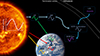 |
Fig. 1. Schematic diagram illustrating the time variation of solar activity and its modulation effect on the GCR transport within the heliosphere. The information regarding solar activity is transmitted to Earth through electromagnetic waves and recorded via the observed SSN and solar radio flux (F10.7). The information regarding solar activity is also carried by the solar magnetic open flux (OF). The cyan arrows illustrate the propagation of the solar activity information within the heliosphere as the solar wind plasma travels away from the Sun. The azure arrows linking the LIS, considered constant in time beyond the heliopause, with the GCR flux, continuously recorded near Earth, indicate that the solar activity information is encoded in the GCR modulation. |
Since the particle velocity and the intensity of the heliospheric transport processes depends on particle rigidity, it is natural to expect that the delay time of GCR modulation is also rigidity-dependent. This has been verified using various methods and observational data (e.g., Shen et al. 2020; Tomassetti et al. 2022; Gong et al. 2025), although results from different analyses are not fully consistent with one another. In this study, we use the force-field approximation to derive an analytical formula for estimating the delay time of GCR modulation and present a quantitative analysis of the rigidity-dependent delay time using information theory. We further employ Monte Carlo methods to evaluate the uncertainty in the above analysis. The LIS and the force-field approximation of GCR modulation are introduced in Sect. 2. We present a simple theoretical analysis of delay time in Sect. 3. The datasets and method used are described in Sect. 4. Subsequently, the results, their physical interpretation, and a comparison with previous studies are discussed in Sect. 5. The summary and conclusion are presented in Sect. 6.
2. LIS and force-field approximation
2.1. LIS
As was mentioned in Sect. 1, the LIS is considered to be isotropic and constant over the timescale concerned here. Earlier studies have attempted to reconstruct the LIS using measurements obtained near Earth (e.g., Matthiä et al. 2013; O’Neill et al. 2015). The Voyager 1 spacecraft crossed the heliopause and entered interstellar space in August 2012 and provided direct flux measurements of low-rigidity particles (< 1 GV protons), which are essential for reconstructing the LIS (Gurnett et al. 2013; Stone et al. 2013). Meanwhile, observations in high-rigidity ranges (> 100 GV protons), from the Alpha Magnetic Spectrometer (AMS-02, Aguilar et al. 2021) experiment and Payload for Antimatter Matter Exploration and Light-nuclei Astrophysics (PAMELA, Adriani et al. 2017) experiment, have helped to constrain the LIS at higher energies. Combining these data, several more reliable LIS functions have recently been developed (e.g., Bisschoff & Potgieter 2016; Corti et al. 2019b; Boschini et al. 2020). According to a LIS comparison presented in Liu et al. (2024), the LIS function proposed by Corti et al. (2019b) is the closest to data for protons, so it is adopted in this study. This LIS is shown in Fig. 2 as a thin black line, with the shaded gray area representing the uncertainty range encompassing three standard deviations.
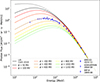 |
Fig. 2. LIS and modulated GCR spectra derived from the force-field approximation. The LIS from Corti et al. (2019b) is shown as a thin black line, with the shaded gray area representing the uncertainty range encompassing three standard deviations. The thick colored lines represent the GCR spectra near 1 AU, calculated using the force-field approximation under different solar modulation potentials. Markers indicate measurements from AMS-02, SOHO/EPHIN, and IMP-8 during different time periods with very similar modulation conditions. In some cases (particularly IMP-8 and AMS-02) vertical bars showing the measurement uncertainties are too small to be seen. The data point with the lowest energy for IMP8 originates from CRNC; it is included in this figure solely for display purposes and is not used in this study. More information about the observational data is listed in Table 1. |
2.2. Force-field approximation
Several empirical, semiempirical, and numerical models for GCR transport have been developed that exhibit varying performances depending on both the type of GCR and the GCR energy ranges (Liu et al. 2024). The force-field approximation of GCRs (Gleeson & Axford 1968; Gleeson & Urch 1973) is a widely used reference model due to its simplicity (Moraal 2013). The force-field approximation for GCR protons is given by:
 (1)
(1)
where E and mp are the kinetic energy and rest energy of the GCR proton in units of mega-electronvolts (MeV), respectively. j(r, E) represents the GCR proton flux with kinetic energy E, measured at a heliocentric distance of r, where r = 1 AU in this study. jLIS(rb, E + Φ) represents the GCR proton flux with kinetic energy E + Φ outside the modulation boundary, rb. Following recent numerical studies (e.g., Boschini et al. 2018; Song et al. 2021), we consider the heliopause to be the boundary of the modulation region, which means rb ≈ 120 AU according to the in situ observation results of the Voyager 1 and Voyager 2 spacecraft (Stone et al. 2013, 2019). Φ, which is in the same unit as proton kinetic energy, is related to the solar modulation potential, ϕ by:
 (2)
(2)
where e is the proton charge, and V(r′) and κr(r′) represent the solar wind speed and the radial dependence of the diffusion coefficient at the heliocentric distance r′, respectively. Equation (2) means that the solar modulation potential contains the integrated effect of the diffusive medium from the heliocentric distance, r, to the GCR modulation boundary, rb (Gleeson & Urch 1973). We note that the use of the standard force-field approximation formula, Eq. (1), assumes that the diffusion coefficient, κ, of GCR particles is directly proportional to the rigidity of the particles, R (κ ∝ R, Moraal 2013), which is a significant constraint on the particle diffusion coefficient. However, in Appendix A we show that our procedure to derive the modulation potential from data, described later in this section, is not affected by the rigidity dependence of the diffusion coefficient.
The thick colored lines in Fig. 2 represent GCR spectra near 1 AU, predicted by the force-field approximation under various solar modulation potentials. The blue markers indicate measurements from AMS-02, the Electron Proton Helium INstrument (EPHIN, Müller-Mellin et al. 1995) on board the Solar and Heliospheric Observatory (SOHO), the Goddard Medium Energy (GME, McGuire et al. 1986) and the Cosmic Ray Nuclear Composition (CRNC, Mason & Mixon 1975) instruments on board the Interplanetary Monitoring Platform-8 (IMP-8) during different time periods, with the vertical blue bars showing the uncertainties in their measurements. It is clear that in August 1999, September 2006, and November 2016, the measured GCR spectra closely align with the approximate force-field spectra when ϕ = 400 MV. Despite the seemingly good agreement in this specific case, discrepancies between the observations and the force-field–approximated spectrum still exist, especially during periods of solar maximum (e.g., Corti et al. 2019a; Zhu & Wang 2025). The reason is that the force-field approximation is too simplistic to fully represent all the modulation processes of GCRs (Caballero-Lopez & Moraal 2004). We also note that, for a fixed time, the low-energy GCRs and high-energy GCRs, such as data in September 2006 detected by SOHO/EPHIN, seem to correspond to different modulation potentials (e.g., Corti et al. 2016; Gieseler et al. 2017; Shen et al. 2021; Long & Wu 2024; Väisänen et al. 2025).
It can be seen that the LIS flux decreases monotonically in the region above tens of mega-electronvolts (MeV). For a given particle’s kinetic energy, E, the right-hand side of Eq. (1) decreases as Φ increases. The measured GCR proton flux can be mapped one-to-one to the solar modulation potential, ϕ, under a specific LIS. This one-to-one mapping implies that the derived solar modulation potential for a certain rigidity uniquely corresponds the measured GCR proton flux. Considering that the relative error in measuring cosmic ray flux is generally greater than 1%, we used Eq. (1) to determine ϕ(R, t) such that
 (3)
(3)
is satisfied. jFFA(ϕ, R, t) and jMeas(R, t) are the particle flux obtained by force-field approximation and measurement at the rigidity, R, and time, t, respectively.
Figure 3(b) illustrates the temporal distribution of solar modulation potential for several energies. It is evident from the figure that there is a positive correlation between the solar modulation potential and the solar activity indices, which are shown in Fig. 3(a). In this study, we used both the measured GCR proton flux and its corresponding solar modulation potential to investigate the GCR modulation delay time. For GCR electrons, we utilized flux exclusively to determine their modulation delay time due to the absence of a reliable LIS, which is necessary to derive the modulation potential. The results are further discussed in Sect. 5.
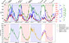 |
Fig. 3. Time evolution of various solar activity indices and derived modulation potential, ϕ, from 1976 to 2022. Panel (a) shows the time profile of monthly solar activity indices, with the SSN, F10.7, and OF represented by solid black, red, and blue lines, respectively. The lower x axis includes solar minimum dates and solar cycle number (solar cycles are separated by gray solid lines). The shaded red and blue areas indicate the periods when the inclination of the heliospheric current sheet (indicated by the tilt angle, solid green line) is less than 70°. The start and end period of each shaded area, along with the corresponding polarity of the heliospheric magnetic field, are marked on the upper x axis. The F10.7 index is plotted in solar flux units (sfu, 1 sfu = 10−22 W m−2 Hz−1). Panel (b) shows the time profile of monthly GCR modulation, ϕ, for protons with different rigidities, derived by measurements of IMP-8, SOHO/EPHIN, and AMS-02, as shown in the legend. |
3. Theoretical derivation of delay time
As was stated in Sect. 1 and introduced by O’Gallagher (1975) and Nagashima & Morishita (1980), the GCR modulation delay time, Δt, can be understood as the combined effect of two components: (1) the finite transport speed of GCRs resulting in Δtp, and (2) the limited speed at which information about the solar activity propagate to the boundary of the heliosphere (which is assumed to be stationary in time) leading to Δts, i.e.,
 (4)
(4)
High-rigidity charged particles in the heliosphere, such as protons with tens of gigavolt (GV) or more, are less affected by heliospheric modulation and can reach Earth by propagating almost ballistically, due to their larger mean free path and corresponding larger diffusion coefficient (Gervasi et al. 1999). Consequently, their corresponding delay time is mostly dominated by the limited propagation speed of the solar activity. In contrast, for lower-rigidity charged particles, such as protons with around 1 GV or less, the delay time is influenced by both effects mentioned earlier. As the particle rigidity decreases, the contribution from Δtp becomes more significant. In short, Δts is independent of the GCR particle rigidity, whereas Δtp depends on the rigidity. Below, we provide a brief theoretical analysis of each.
3.1. Delay time, Δts, due to solar wind transport
To start with, we assume that the temporal variation of solar activity recorded near the solar surface is represented by S(t)≡S(r = rS, t), and that the information about solar activity propagates outward at a constant speed, V. The solar activity signal observed at a heliocentric distance, r, can then be expressed as S(r, t) = S(t − r/V). Inspired by Gleeson & Axford (1968), Slaba & Whitman (2020), we express the diffusion coefficient of a particle with rigidity R at time t and position r as:
 (5)
(5)
where κ0 is a normalization factor, κR accounts for the rigidity dependence, κr captures the radial dependence, and α(r) is the power-law index characterizing the radial variation of the diffusion coefficient at location r. By substituting κr from Eq. (5) into Eq. (2), we obtain the following expression for the solar modulation potential:
 (6)
(6)
In order to make analytical derivations, here we assume that the solar activity signal varies sinusoidally, i.e., S(t) = sin(2πt/T), with T ≈ 11 years. Then Eq. (6) becomes:
 (7)
(7)
with
 (8)
(8)
 (9)
(9)
 (10)
(10)
By comparing Eq. (7) with S(t) = sin(2πt/T), we identify the phase shift, θ, as the modulation delay time of the solar modulation potential at r relative to the solar activity index:
 (11)
(11)
For a typical solar wind speed of V ≈ 450 km/s, VT ≫ rb ≫ r is valid. Then we can simplify the calculation of Eqs. (8) and (9) by expanding the trigonometric terms at first order in (2πr′)/(VT). Due to the complex nature of Eqs. (8) and (9) in the case of arbitrary α(r), we assume no radial dependence, i.e., α(r) = α, which is a good approximation of the behavior derived from turbulence theory (see, e.g., Ngobeni 2015, Figs. 3.3 and 3.4) and references therein). Equation (11) reduces to:
 (12)
(12)
As a result, Eq. (12) shows that the delay time, Δts, is determined by the characteristic size, rb, of the GCR modulation region, the propagation speed, V, of solar activity information through the heliosphere, and the distribution of the diffusion coefficient with respect to radial distance. More specifically, if we set α = 0, then Δts ≈ rb/(2V), which is about 7.7 months when V ≈ 450 km/s and rb ≈ 120 AU. This ultimately manifests as the phase difference between the solar modulation potential and the solar activity signal and is analogous to the findings obtained through perturbation analysis in Chih & Lee (1986).
3.2. Delay time, Δtp, due to GCR particle transport
The transport process of GCRs in the heliosphere involves several factors (e.g., Jokipii 1989), including diffusion, convection, adiabatic energy losses, and drifts, all of which contribute to the modulation delay time. A comprehensive theoretical analysis that simultaneously accounts for all these effects is highly complex and beyond the scope of this study. Therefore, we followed the approach of Parker (1965) and focused specifically on the contribution of diffusion and convection effects to the delay time. The transport of GCR scattering centers from the edge of the heliosphere to its inner regions can be described as the superposition of two effects: inward diffusion and outward convection. The net velocity of this transport process is the vector sum of the diffusion and convection velocities. According to the definition of the diffusion coefficient and the analysis conducted by Strauss et al. (2011), the rigidity-dependent GCR delay time can be approximated by the sum of the equivalent diffusion time, td, and the typical solar wind convection time, tc:
![Mathematical equation: $$ \begin{aligned} \Delta t_\mathrm{p} \approx \left[t_\mathrm{d} ^{-1}-t_\mathrm{c} ^{-1}\right]^{-1}=\left[t_\mathrm{d} ^{-1}-\frac{V}{r_\mathrm{b} }\right]^{-1}. \end{aligned} $$](/articles/aa/full_html/2025/12/aa57157-25/aa57157-25-eq13.gif) (13)
(13)
We note that for diffusion coefficients that do not vary with radial distance, i.e., when α = 0, the particle diffusion time can be expressed as td = rb2/(6κ) as was adopted in previous studies (Strauss et al. 2011; Tomassetti et al. 2022). However, for the more general case of α ≠ 0, the one-dimensional average quadratic spatial displacement for a GCR particle undergoing diffusion with κr = rα is ⟨r2⟩ ∼ (κ0κRt)2/(2 − α) according to the theoretical analysis of Fa & Lenzi (2003). We can thus infer that the average timescale associated with diffusion from the heliopause to Earth is td ∼ rb2 − α/κ0κR, which can be expressed more accurately as:
 (14)
(14)
where Γ represents the gamma function. When α ∈ (0.60, 0.95), we find that τ(α)∈(1.13, 0.75); therefore, we no longer consider τ(α) to be an independent parameter and fit  as a combined parameter.
By adopting different functional forms for κR, we can use Eq. (13) to explore various relationships between the delay time and particle rigidity. In addition, this equation offers a method of estimating rigidity-dependent diffusion coefficients based on the rigidity-dependent delay time. We adopted the double power law form of κR that is widely used in numerical studies of GCR transport to fit the rigidity-dependent delay time (e.g., Corti et al. 2019b). For more detailed results, please refer to Sect. 5.2.
4. Datasets and method
4.1. Datasets
As is illustrated in Fig. 1, several parameters can serve as real-time proxies for solar activity. Based on the following criteria, we chose the SSN, F10.7, and OF as reference indices for estimating the GCR modulation delay time. First, these solar activity indices have been continuously recorded for more than four solar cycles, providing sufficient invaluable data for our analysis. Second, they capture the global effects of solar activity on the heliosphere. Finally, using these widely adopted indices ensures consistency with previous studies, which is critical for validating the estimated delay time. Figure 3(a) illustrates the monthly SSN, F10.7, and OF parameters, which are plotted as black, red, and blue lines, respectively. The shaded red and blue areas indicate the periods when the inclination of the heliospheric current sheet is less than 70°, which define the calculation windows for A− and A+ polarity periods in this study.
The SSN data were accessed from the World Data Center SILSO1, Royal Observatory of Belgium, Brussels (SILSO World Data Center 1974-2025). The F10.7 data were provided by the Canadian Solar Radio Monitoring Program2 (Tapping 2013). The OF data were derived by the current sheet-source surface Model (CSSS Model, Zhao & Hoeksema 1995) based on the line-of-sight photospheric magnetic fields observed by the Wilcox Solar Observatory3 (WSO, Duvall et al. 1977). Using the WSO synoptic charts as input, we applied spherical harmonic functions up to the ninth order to reconstruct the coronal magnetic field. Magnetic field lines extending up to 2.5 solar radii are considered as open magnetic field lines. By leveraging the resolution of the WSO synoptic charts, we can calculate the open magnetic flux of the entire Sun.
Although several spacecraft have measured the temporal variation of GCR flux over recent decades, no single mission has covered more than four solar cycles (matching the coverage of the solar activity indices) while maintaining high energy resolutions for GCRs. For this reason, we combined data from different spacecraft covering different time periods and energy ranges. Table 1 summarizes the instruments used in this work, data collection periods, rigidity ranges, and relevant references. Notably, the PAMELA data were excluded from the subsequent delay time analysis, as the spacecraft did not span a complete solar cycle, which limits its applicability when studying the long-term GCR modulation delay time based on our method. We computed monthly averages of all GCR measurements to align them with the time resolution of solar activity indices. Data influenced by solar energetic particle events were excluded from the averaging process to ensure that the derived modulation delay time reflects only the long-term modulation effects of the solar activity.
Basic information regarding the GCR flux measurement data used in this study.
4.2. Method
As is described in Sect. 1, the Pearson correlation coefficient (PCC, Pearson 1895) is widely used to quantify the strength of the linear association between two variables and is commonly applied to determine the delay time of GCR modulation. The PCC typically measures the degree of correlation between two variables on a linear scale (Ratner 2009). However, the relationship between solar activity and GCR modulation involves complex, nontrivial physical processes, including the propagation and evolution of IMF turbulence in the heliosphere, particle diffusion, drift motions, and adiabatic cooling processes that affect the transport of GCRs (e.g., Jokipii et al. 1977). Therefore, establishing a linear correlation between them becomes challenging. A more comprehensive method capable of capturing nonlinear associations is needed. In this context, we turn to the concept of mutual information.
In 1948, Claude E. Shannon first introduced the concept of information entropy (Shannon 1948). Based on his pioneering work, information theory has made significant foundational contributions across various fields (e.g., Cover 1999). While the nature of “information” remains complex, information theory provides a quantitative method to measure it.
A central concept is mutual information (e.g., Kraskov et al. 2004), which quantifies the amount of information shared between two random variables, X and Y, over the domain 𝕏 × 𝕐:
 (15)
(15)
where p(x) and p(y) represent the marginal probability density functions of X and Y, respectively, and p(x, y) is their joint probability density function. Generally, if X and Y are statistically independent, then p(x, y) = p(x)p(y), resulting in I(X; Y) = 0, which indicates that X and Y do not share information. On the other hand, a larger I(X; Y) implies that the variables share more information, which also implies a stronger association, whether linear or nonlinear in nature. Following the analysis presented in Sect. 1 and illustrated in Fig. 1, we calculated the mutual information between the solar activity index and GCR data by shifting the time of the solar activity index within the calculation window. The optimal delay time then corresponds to the shift for which the mutual information reaches the maximum value.
As can be seen from Eq. (15), an accurate computation of mutual information critically depends on a reliable estimation of the joint probability density function, p(x, y), which can be challenging, especially with a limited sample size of observational data. A straightforward estimation technique for p(x, y) is the histogram (data-bins) method, which partitions data into a series of preset bins and counts the number of samples falling within each bin. Note that the data-bin method can be sensitive to the chosen bin size, particularly when applied to small datasets (e.g., Wȩglarczyk 2018). In this case, a more robust approach is the kernel density estimation (KDE, Parzen 1962; Chen 2017), which estimates the probability density function as:
 (16)
(16)
where  is the estimated probability distribution, xi is i-th of the n data samples from an unknown distribution p(x), and K denotes the kernel function with a bandwidth of h. We adopted h ≈ n−1/6 in accordance with the rule of thumb for bandwidth selection in Bashtannyk & Hyndman (2001).
In the process of averaging the data used here into monthly values, there are generally enough statistics to satisfy a Gaussian distribution. Consequently, the central limit theorem supports the choice of a Gaussian kernel, defined by:
 (17)
(17)
where ζ is the input value of Gaussian kernel function. This approach in Eqs. (15)–(17) enables us to better quantify the degree of statistical dependence between solar activity indices and GCR fluxes, including their potential nonlinear correlations, providing a more complete characterization of the modulation delay time.
Figure 4 illustrates the joint probability distribution between solar activity indices and the modulation potential, ϕ, for protons (1.00–1.92 GV), derived from AMS-02 data covering the period from April 2014 to May 2022. Both the data-bin (first and third rows) and KDE (second and forth rows) methods were employed. In our analysis, we fixed the GCR modulation potential ϕ data within the specified time window and systematically shifted the solar activity index by monthly steps. For each shift, we calculated the mutual information and correlation coefficient within the window and identify the time shift that maximizes these measures. The number of months corresponding to this maximum was then interpreted as the delay time of GCR modulation within the window. As is demonstrated clearly in Fig. 4, the KDE method enhances the saliency of the joint distribution while preserving the characteristics of the data-bin method. We calculated the mutual information by shifting the solar activity index from −15 months to 30 months. A negative value indicates a shift to the future, while a positive value indicates a shift to the past. Selected results for four time shifts are illustrated in the four columns of Fig. 4. In the second column, mutual information reaches its peak with a 5-month shift in F10.7 and a 2-month shift in OF with respect to ϕ. During this period, when the IMF polarity is positive, we define the time lags of GCRs modulation behind the F10.7 index by ∼5 months and behind the OF index by ∼2 months. Results obtained using the SSN (not shown) as the solar activity index are similar to those of the F10.7 index.
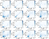 |
Fig. 4. Examples of the joint probability distribution between the modulation potential, ϕ(R), for protons (1.00–1.92 GV, AMS-02 data) and solar activity indices including F10.7 (first and second rows) and OF (third and fourth rows) spanning from April 2014 to May 2022. The first and third rows show results obtained using the data-bin method, while the second and fourth rows are obtained by the KDE method. For each method, we fixed ϕ(R) and shifted the solar activity index, with positive values (month) representing shifts to the past while negative values representing shifts to the future. The shift time is, from left to right, −15, 5, 15, and 30 months for F10.7 (upper two rows) and −15, 2, 15, and 30 months for OF (lower two rows). In the second column, mutual information reaches its peak when offset by 5 months in F10.7 and by 2 months in OF relative to ϕ, thereby defining the delay time. |
Additionally, we examined the results from the cross-correlation method in comparison to those from the mutual information method. Figure 5 illustrates the profile of the cross-correlation coefficient and mutual information by shifting F10.7 with AMS-02 proton data fixed. It can be found that the cross-correlation coefficient is flatter near the peak position compared to mutual information, indicating that the mutual information method is more sensitive to the selection of the peak position and is more suitable for determining delay time in nonlinear correlation processes than the cross-correlation method, especially when the temporal resolution of measurement data is suboptimal.
 |
Fig. 5. Comparison of two methods of determining delay time. Panel (a) shows the cross-correlation coefficient by shifting F10.7 index to the future with AMS-02 proton data fixed. Panel (b) is the same with panel (a) but using mutual information method based on Eq. (15). |
Furthermore, we adopted a Monte Carlo method to assess the uncertainty of the GCR delay time derived above. We generated 500 new sets of GCR flux–time data by Gaussian sampling, using the measured GCR fluxes and their uncertainties as means and standard deviations, respectively. For each realization, we repeated the method described in the previous paragraph to calculate the delay time. Figure 6 shows representative results using this approach and the AMS-02 data. In each panel, the shaded blue histogram illustrates the distribution of estimated GCR delay time, and the solid red curve represents the best-fit Gaussian distribution. As outputs, the GCR delay time and its variance are parameters, as denoted by μ and σ in Fig. 6(a).
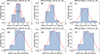 |
Fig. 6. Delay time of modulation potential versus F10.7 or OF and its uncertainty obtained using the Monte Carlo method, based on AMS-02 data. In each panel, the shaded blue histogram illustrates the distribution of delay time, and the solid red curve represents the best-fit Gaussian distribution. The output delay time and its variance were determined from the Gaussian fit parameters, labeled as μ and σ in panel (a). Abbreviations: MI = mutual information method. |
5. Results and discussion
5.1. Key results of the modulation delay time relative to OF
Figure 7 shows the derived delay time of GCR modulation, ϕ (or flux), relative to the OF by mutual information method, based on data recorded by IMP-8, SOHO/EPHIN, and AMS-02 during different periods. Due to the lack of a reliable LIS for GCR electrons, the delay time corresponding to its modulation potential is not included here. Key findings are listed below.
-
As is illustrated in Fig. 7, regardless of the IMF polarity (A− or A+), the GCR modulation delay time relative to OF decreases with the GCR rigidity, based on results from all three instruments. The theoretical explanation of this rigidity dependence is given below in Sect. 5.2.
-
Based on AMS-02 measurements, the derived GCR proton delay time using either ϕ or fluxes, shown in panel (c), is mostly consistent, except for the lowest rigidity. As particle rigidity increases, the modulation delay time of GCR protons and electrons gradually approaches a constant value. This delay time, which is independent of particle rigidity, is referred to as Δts related to solar wind propagation (see Sect. 3).
-
Panels (a) and (c) show that periods with qA < 0 exhibit a longer delay time than those with qA > 0, in agreement with previous findings (e.g., Nymmik 2000; Shen et al. 2020). Here q is the GCR particle charge, and A = 1 (or −1) if the solar magnetic field is predominantly outward (or inward) at the solar north pole.
The fact that delay time is related to qA can be attributed to particle drifts in the heliosphere. When qA > 0, GCRs are more likely to drift inward via the polar region where the solar wind speed is higher (McComas et al. 2000), resulting in a shorter delay time, Δts, as is described by Eq. (12). When qA < 0, GCR preferentially move along the heliospheric current sheet toward Earth, resulting in a longer transport path for particles compared to the case when qA > 0 (Strauss et al. 2011), which leads to an increased transport time, Δtp.
The uncertainty in the delay time shown in Fig. 7 arises from two major sources. One source is the uncertainties associated with the GCR measurements, especially for SOHO/EPHIN as is illustrated in Fig. 2, mostly due to the specific data acquisition method based on inversion methods rather than direct measurements (Kühl et al. 2016). The other reason is that the highest resolution available is monthly for most datasets used here.
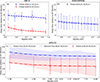 |
Fig. 7. Delay time of GCR modulation with respect to the OF, derived using mutual information, for protons measured by IMP-8, SOHO/EPHIN, AMS-02 and electrons measured by AMS-02 in different time periods (panels (a)–(c), respectively). The delay time and associated uncertainty derived from the modulation potential are shown with markers and error bars. The shaded red and blue areas in panel (c) represent the delay time derived directly from AMS-02 proton and electron data, respectively. The dashed lines in panels (a) and (b) and the dash-dotted lines in panel (c) are the fit delays obtained using the format of κR in Eq. (19), detailed in Sect. 5.2. |
5.2. Rigidity dependence of delay time
Following the derivation presented in Sect. 3, the modulation delay time of GCRs can be expressed as:
![Mathematical equation: $$ \begin{aligned} \Delta t =\Delta t_\mathrm{s} +\Delta t_\mathrm{p} \approx \left|\frac{ 1-\alpha }{2-\alpha }\right|\frac{r_\mathrm{b} }{V} + \left[\frac{(2-\alpha )^{2}\kappa _0\, \kappa _R}{r_\mathrm{b} ^{2-\alpha }}-\frac{V}{r_\mathrm{b} }\right]^{-1} , \end{aligned} $$](/articles/aa/full_html/2025/12/aa57157-25/aa57157-25-eq20.gif) (18)
(18)
with V = 450 km/s and rb = 120 AU. From Eq. (18), we can see that as the rigidity of the GCRs increases, the diffusion coefficient, κR, increases, leading to a gradual decrease in Δtp. As Δtp approaches zero, the delay time, Δt, will be primarily influenced by Δts. Conversely, as the particle rigidity decreases, the inward diffusion of GCRs decreases (κR term), while the solar wind term (−V/rb) becomes more important and Δtp increases. Consequently, the modulation delay time, Δt, increases as GCR energy decreases.
For the rigidity dependence of the diffusion coefficient, κR, we adopted a double power-law form that is widely used in numerical studies of GCR transport (e.g., Potgieter et al. 2014; Corti et al. 2019b; Fiandrini et al. 2021; Song et al. 2021):
![Mathematical equation: $$ \begin{aligned} \kappa _R(R) = \left(\frac{R}{R_{k}}\right)^{a} \left[1 + \left(\frac{R}{R_{k}}\right)^{c}\right]^{\frac{b-a}{c}}, \end{aligned} $$](/articles/aa/full_html/2025/12/aa57157-25/aa57157-25-eq21.gif) (19)
(19)
where Rk is the break rigidity between the two power laws, a and b are the low- and high-rigidity power-law indices, respectively, and c controls the smoothness of the transition between the low- and high-rigidity parts. Based on results from previous numerical studies (Song et al. 2021), we adopted Rk = 4 GV and c = 3. The AMS-02 data used here cover rigidity between 1.39 and 9.66 GV, which allows for the fitting of κR using the double power law, while data from IMP-8 and SOHO/EPHIN only cover the lower-rigidity part of the function. Combining Eqs. (18) and (19), we fit the delay time derived from data to obtain parameters constraining the analytical delay time including κR, κ0, and α. The fitting parameters are summarized in Table 2. The theoretical delay time in Eq. (18) as a function of rigidity is plotted as dashed lines in Fig. 7(a)(b) and dash-dotted lines in Fig. 7(c).
Fitting parameters of rigidity-dependent GCR modulation delay time with respect to magnetic OF.
Using the delay time derived from SOHO/EPHIN and AMS-02, we obtained the fit κ0 and κR with power-law indices a and b. Our results (last three rows of Table 2) agree nicely with those reported in previous numerical studies, (see, e.g, Fig. 5 of Corti et al. 2019b, Fig. 10 of Fiandrini et al. (2021), and Fig. 4 of Song et al. 2021). This suggests that the rigidity dependence of the diffusion coefficient can be well described by a double power-law function. Furthermore, most numerical studies set the diffusion coefficient inversely proportional to the strength of the IMF, i.e., α is close to 1 (see Eq. (5)). Our results support this assumption, but are slightly smaller than one.
For the delay time of IMP-8, the fitting parameters are quite different from those of SOHO/EPHIN and AMS-02, especially for periods of qA < 0. This may be attributed to the limitations of the force-field approximation in the low rigidity range (0.3–0.8 GV, or 60–300 MeV for protons). According to the discussions in Gleeson & Axford (1968) and Fisk & Axford (1969), the force field approximation is more reliable for high-rigidity particles, which are less modulated. The validity condition is  , where the tilde denotes a characteristic value. Besides, the unavoidable interference from transient events within the heliosphere, such as Forbush decrease due to solar magnetic eruptions, may have influenced the results more at lower energies observed by IMP-8.
5.3. Results of the modulation delay time relative to SSN (or F10.7)
In additional to OF, we derived the delay time of GCR modulation with other solar activity indices, including SSN and F10.7. The results from SSN are shown in Fig. 8, while those from F10.7 are similar but not shown.
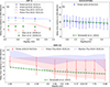 |
Fig. 8. Delay time of GCR modulation with respect to the SSN, derived using mutual information. The meaning of red and blue markers and shaded bands is the same as in Figure 7. We also include results from previous works by Shen et al. (2020), Tomassetti et al. (2022), shown as green markers and lines. To ensure consistency for comparison, the calculation window for determining delay time in panel (a) has been adjusted as follows: A < 0 covers June 1980 to September 1989, and A > 0 covers April 1991 to June 1999. The relatively small error bars in panel (a) result from the lower uncertainty of the IMP-8 data compared to the SOHO/EPHIN and AMS-02 data. |
By comparing Figs. 7 and 8, we can find that the delay time of GCR modulation derived from the OF is different from that derived from the SSN. The delay time relative to the SSN is about 5 months systematically longer than that relative to the OF, which aligns well with the conclusion of Wang et al. (2022), implying that the solar activity level in the photosphere requires some months to be reflected in the open magnetic flux, which subsequently influences the transport of GCR particles in the heliosphere. More comparisons with previous studies, mainly based on SSN, are given in Sect. 5.4.
We stress that the delay time between SSN and modulation provides an advanced forecasting window for the GCR modulation process. For instance, the maximum delay time between them can be about 1 year, and this may give more time to plan for future human deep space exploration programs.
5.4. Comparison of delay time results with previous studies
Nymmik & Suslov (1995) employed three different methods to derive the temporal evolution of the delay time and found it to be longer in odd cycles than in even ones. A couple of factors may contribute to this phenomenon. A longer delay time between OF and SSN during odd cycles may be one of the reasons for the extended delay between SSN and GCR modulation, as discussed in Wang et al. (2022). Besides, it can be seen in Fig. 3 that odd solar cycles include a longer qA < 0 period, whereas even solar cycles contain a longer qA > 0 period (more in Sect. 5.1). Additionally, to obtain the delay time related to particle rigidity, both Nymmik & Suslov (1995) and Nymmik (2000) used data from ground-based neutron detectors and stratospheric charged-particle counting rates, which limits the energy resolution of cosmic ray flux measurements. This limitation may contribute to the discrepancies between their findings and the results of this study.
Shen et al. (2020) employed the cross-correlation method and utilized GCR flux data from IMP-8 to determine that the GCR modulation delay time relative to SSN decreases as the particle rigidity increases for both qA > 0 and qA < 0 periods. To better compare our results with Shen et al. (2020), we repeated our mutual information analysis, using both ϕ and the proton flux, in the same time intervals as used by Shen et al. (2020). The comparison is presented in Fig. 8, panel (a). We see some differences, especially for qA > 0 periods, which, in addition to the different methods used to compute the delay (mutual information vs. cross-correlation) can be attributed to a couple of causes. First, they applied a low-pass filter on daily IMP-8 data and smoothed the SSN, whereas we calculated the monthly average of SSN data without any filtering or smoothing. Second, the choice of start and end time, as well as the duration of the calculation window, may influence the derived delay time.
Koldobskiy et al. (2022) utilized data from both ground-based neutron detectors and space-borne spectrometers (PAMELA and AMS-02) to investigate the delay time of cosmic ray modulation in relation to the SSN and the OF using cross-correlation and wavelet coherence methods. They found that the time lag of the combined neutron monitor records with respect to SSN depicts a clear bimodal distribution: a delay time longer during qA < 0 than qA > 0 as we have discussed in Sect. 5.1. However, no clear dependence of the delay time on the particle rigidity was observed. This lack of significance may be attributed to the limited rigidity resolution of ground-based neutron detectors and limited data from PAMELA and AMS-02. Additionally, the neutron detectors are sensitive to a rigidity range above a few gigavolt (GV), where the delay time approaches a constant value according to our analysis in Sect. 5.2.
Tomassetti et al. (2022) combined data from space-based instruments (IMP-8/GME and ACE/Cosmic-Ray Isotope Spectrometer) and ground-based neutron detectors using the cross-correlation method to establish empirical relationships between delay time relative to SSN for different particle rigidities and periods. Moreover, the GCR modulation delay time, described by Tomassetti et al. (2022), is attributed to the rigidity-dependent properties of particle diffusion processes in agreement with our theoretical derivations in Sect. 3.2. We compared the rigidity-related delay time fit by Tomassetti et al. (2022) with our calculated results shown in Fig. 8(b)(c). Both studies use the GCR modulation potential, ϕ, to calculate the delay time, and the results obtained show good agreement within the rigidity range of 1–10 GV. They accounted for the uncertainty introduced by the LIS and SSN smoothing algorithms in their calculations but did not consider the uncertainty of GCR measurement, which may explain their relatively small delay time uncertainty (see Fig. 8 of Tomassetti et al. 2022).
Recently, Gong et al. (2025) studied the time lag between solar polar magnetic field and daily AMS-02 proton flux using the cross-correlation method and found a decrease in the delay time with particle rigidity. The quantitative comparison with our results is not straightforward, since different solar indices are used in two studies. But the slope of the decrease is comparable (as can be seen by comparing Fig. 6 of Gong et al. (2025) and Fig. 8 here).
6. Summary and conclusion
In this paper, we have quantitatively investigated the rigidity-dependent delay time in the modulation of GCRs using an information-theory approach. For the nonlinear process of GCR modulation, we applied mutual information to determine the delay time and estimate its uncertainty via Monte Carlo methods. Using long-term GCR observations collected since the 1970s by various space missions, we innovatively derived and analyzed the distribution of modulation delay time in relation to the open magnetic flux of the Sun over a wide rigidity range from 0.3 to 10 GV.
Meanwhile, by adopting the force-field and particle diffusion approximations, we presented an analytical formula for estimating the GCR modulation delay time. We then fit the data-derived delay time with a widely accepted expression for the rigidity-dependent diffusion coefficient and validated our results against previous numerical studies. Through the derivation presented in Sect. 3 and Appendix A, we have extended the application of the force field approximation to quasi-static processes that change slowly over time, as well as to a arbitrary continuous rigidity-dependent diffusion coefficient.
Additionally, we have provided a physical explanation and quantitative description for the nonzero GCR modulation delay time (Δts) observed at a high rigidity range. Although the force field approximation serves as an approximate analytical model, it offers a reasonable reliable method of understanding the modulation process of GCRs, complementing numerical models.
Finally, we look forward to future space instrumentation with higher temporal resolutions, longer time spans, more spatial coverage, and better energy resolutions and coverage that will help deepen our knowledge of the GCR modulation process. This will also advance our understanding of the heliosphere’s structure and the mechanisms driving the long-term space radiation environment.
Data availability
IMP-8 data can be downloaded directly from the Space Physics Data Facility: https://spdf.gsfc.nasa.gov/pub/data/imp/imp8/particles_uchi/hourly and https://spdf.gsfc.nasa.gov/pub/data/imp/imp8/particles_gme/data/flux/gme_h0. SOHO/EPHIN data are available on http://ulysses.physik.uni-kiel.de/costep/level3/penetrating/. AMS-02 data used in this study can be downloaded from https://ams02.space/publications/202402. Details and instructions about the SSN, F10.7, and OF datasets can be found in Sect. 4.1.
Acknowledgments
The authors thank Ian G. Richardson, Marek Siluszyk and Zhenning Shen for helpful discussions and thank the anonymous reviewer for his/her time and effort in helping us improve this paper. The authors acknowledge the support by the National Natural Science Foundation of China (Grant Nos. 42188101, 42521007, 42474221).
References
- Adriani, O., Barbarino, G. C., Bazilevskaya, G. A., et al. 2017, Riv. Nuovo Cim., 40, 473 [Google Scholar]
- Aguilar, M., Cavasonza, L. A., Ambrosi, G., et al. 2021, Phys. Rep., 894, 1 [NASA ADS] [CrossRef] [Google Scholar]
- Aguilar, M., Ambrosi, G., Anderson, H., et al. 2025, Phys. Rev. Lett., 134, 051002 [Google Scholar]
- Bashtannyk, D. M., & Hyndman, R. J. 2001, Comput. Stat. Data Anal., 36, 279 [Google Scholar]
- Bisschoff, D., & Potgieter, M. S. 2016, Ap&SS, 361, 48 [NASA ADS] [CrossRef] [Google Scholar]
- Blandford, R. D., & Ostriker, J. P. 1978, ApJ, 221, L29 [Google Scholar]
- Boschini, M., Della Torre, S., Gervasi, M., La Vacca, G., & Rancoita, P. 2018, Adv. Space Res., 62, 2859 [Google Scholar]
- Boschini, M., Della Torre, S., Gervasi, M., et al. 2020, ApJS, 250, 27 [NASA ADS] [CrossRef] [Google Scholar]
- Caballero-Lopez, R. A., & Moraal, H. 2004, J. Geophys. Res.: Space Phys., 109 [Google Scholar]
- Chen, Y.-C. 2017, Biostat. Epidemiol., 1, 161 [Google Scholar]
- Chih, P. P., & Lee, M. A. 1986, J. Geophys. Res.: Space Phys., 91, 2903 [Google Scholar]
- Corti, C., Bindi, V., Consolandi, C., & Whitman, K. 2016, ApJ, 829, 8 [Google Scholar]
- Corti, C., Bindi, V., Consolandi, C., et al. 2019a, in Proceedings of 36th International Cosmic Ray Conference – PoS (ICRC2019) (SISSA Medialab), 358, 1070 [Google Scholar]
- Corti, C., Potgieter, M. S., Bindi, V., et al. 2019b, ApJ, 871, 253 [NASA ADS] [CrossRef] [Google Scholar]
- Cover, T. M. 1999, Elements of Information Theory (John Wiley& Sons) [Google Scholar]
- Duvall, T. L., Wilcox, J. M., Svalgaard, L., Scherrer, P. H., & McIntosh, P. S. 1977, Sol. Phys., 55, 63 [Google Scholar]
- Fa, K. S., & Lenzi, E. K. 2003, Phys. Rev. E, 67, 061105 [Google Scholar]
- Fiandrini, E., Tomassetti, N., Bertucci, B., et al. 2021, Phys. Rev. D, 104, 023012 [NASA ADS] [CrossRef] [Google Scholar]
- Fisk, L., & Axford, W. 1969, J. Geophys. Res., 74, 4973 [NASA ADS] [CrossRef] [Google Scholar]
- Forbush, S. E. 1958, J. Geophys. Res., 63, 651 [CrossRef] [Google Scholar]
- Gervasi, M., Rancoita, P., Usoskin, I., & Kovaltsov, G. 1999, Nucl. Phys. B, Proc. Suppl., 78, 26 [Google Scholar]
- Gieseler, J., Heber, B., & Herbst, K. 2017, J. Geophys. Res.: Space Phys., 122, 10964 [Google Scholar]
- Gleeson, L., & Axford, W. 1968, ApJ, 154, 1011 [NASA ADS] [CrossRef] [Google Scholar]
- Gleeson, L., & Urch, I. 1973, Ap&SS, 25, 387 [Google Scholar]
- Gong, S., Duan, L., Zhao, J., et al. 2025, Phys. Rev. D, 111, 083050 [Google Scholar]
- Gurnett, D., Kurth, W., Burlaga, L., & Ness, N. 2013, Science, 341, 1489 [NASA ADS] [CrossRef] [Google Scholar]
- Hathaway, D. H. 2015, Liv. Rev. Sol. Phys., 12, 1 [CrossRef] [Google Scholar]
- Iskra, K., Siluszyk, M., Alania, M., & Wozniak, W. 2019, Sol. Phys., 294, 115 [Google Scholar]
- Jokipii, J. 1989, Adv. Space Res., 9, 105 [Google Scholar]
- Jokipii, J., Levy, E., & Hubbard, W. 1977, ApJ, 213, 861 [CrossRef] [Google Scholar]
- Koldobskiy, S. A., Kähkönen, R., Hofer, B., et al. 2022, Sol. Phys., 297, 38 [Google Scholar]
- Kraskov, A., Stögbauer, H., & Grassberger, P. 2004, Phys. Rev. E, 69, 066138 [NASA ADS] [CrossRef] [Google Scholar]
- Kühl, P., Gómez-Herrero, R., & Heber, B. 2016, Sol. Phys., 291, 965 [Google Scholar]
- Liu, W., Guo, J., Zhang, J., & Semkova, J. 2023, ApJ, 949, 77 [Google Scholar]
- Liu, W., Guo, J., Wang, Y., & Slaba, T. C. 2024, ApJS, 271, 18 [Google Scholar]
- Lockwood, J., & Webber, W. 1984, J. Geophys. Res.: Space Phys., 89, 17 [Google Scholar]
- Long, W.-C., & Wu, J. 2024, Phys. Rev. D, 109, 083009 [Google Scholar]
- Marsch, E. 2006, Liv. Rev. Sol. Phys., 3, 1 [Google Scholar]
- Mason, G. M., & Mixon, W. W. 1975, University of Chicago charged particle experiments on IMP-7 and IMP-8 - instrument and data format descriptions, Technical Report B23906–000A, U. of Chicago, Enrico Fermi Inst., Lab. for Astrophys. and Space Res., Chicago, IL [Google Scholar]
- Matthiä, D., Berger, T., Mrigakshi, A. I., & Reitz, G. 2013, Adv. Space Res., 51, 329 [CrossRef] [Google Scholar]
- McComas, D., Barraclough, B., Funsten, H., et al. 2000, J. Geophys. Res.: Space Phys., 105, 10419 [Google Scholar]
- McGuire, R. E., von Rosenvinge, T. T., & McDonald, F. B. 1986, ApJ, 301, 938 [Google Scholar]
- Mishra, V., & Mishra, A. 2018, Sol. Phys., 293, 1 [NASA ADS] [CrossRef] [Google Scholar]
- Moraal, H. 2013, Space Sci. Rev., 176, 299 [CrossRef] [Google Scholar]
- Müller-Mellin, R., Kunow, H., Fleißner, V., et al. 1995, Sol. Phys., 162, 483 [Google Scholar]
- Nagashima, K., & Morishita, I. 1980, Planet. Space Sci., 28, 195 [Google Scholar]
- Ngobeni, M. D. 2015, Ph.D. Thesis, the Potchefstroom Campus of the North-West University [Google Scholar]
- Nymmik, R. 2000, Adv. Space Res., 26, 1875 [Google Scholar]
- Nymmik, R., & Suslov, A. 1995, Adv. Space Res., 16, 217 [Google Scholar]
- O’Gallagher, J. 1975, ApJ, 197, 495 [CrossRef] [Google Scholar]
- O’Neill, P., Golge, S., & Slaba, T. 2015, NASA Technical Paper, 218569 [Google Scholar]
- Parker, E. N. 1965, Planet. Space Sci., 13, 9 [Google Scholar]
- Parzen, E. 1962, Ann. Math. Stat., 33, 1065 [Google Scholar]
- Pearson, K. 1895, Proc. Roy. Soc., 58, 240 [Google Scholar]
- Potgieter, M. S. 2013, Liv. Rev. Sol. Phys., 10, 1 [Google Scholar]
- Potgieter, M., Vos, E., Boezio, M., et al. 2014, Sol. Phys., 289, 391 [NASA ADS] [CrossRef] [Google Scholar]
- Ratner, B. 2009, J. Target. Meas. Anal. Mark., 17, 139 [Google Scholar]
- Shannon, C. E. 1948, Bell Syst. Tech. J., 27, 379 [Google Scholar]
- Shen, Z., Qin, G., Zuo, P., Wei, F., & Xu, X. 2020, ApJ, 900, 143 [NASA ADS] [CrossRef] [Google Scholar]
- Shen, Z., Yang, H., Zuo, P., et al. 2021, ApJ, 921, 109 [Google Scholar]
- SILSO World Data Center 1974-2025, International Sunspot Number Monthly Bulletin and Online Catalogue [Google Scholar]
- Slaba, T. C., & Whitman, K. 2020, Space Weather, 18, e2020SW002456 [CrossRef] [Google Scholar]
- Song, X., Luo, X., Potgieter, M. S., Liu, X., & Geng, Z. 2021, ApJS, 257, 48 [NASA ADS] [CrossRef] [Google Scholar]
- Stone, E., Cummings, A., McDonald, F., et al. 2013, Science, 341, 150 [NASA ADS] [CrossRef] [Google Scholar]
- Stone, E. C., Cummings, A. C., Heikkila, B. C., & Lal, N. 2019, Nat. Astron., 3, 1013 [NASA ADS] [CrossRef] [Google Scholar]
- Strauss, R., Potgieter, M., Kopp, A., & Büsching, I. 2011, J. Geophys. Res.: Space Phys., 116 [Google Scholar]
- Tapping, K. 2013, Space Weather, 11, 394 [CrossRef] [Google Scholar]
- Thomas, S. R., Owens, M. J., & Lockwood, M. 2014, Sol. Phys., 289, 407 [Google Scholar]
- Tomassetti, N., Bertucci, B., & Fiandrini, E. 2022, Phys. Rev. D, 106, 103022 [CrossRef] [Google Scholar]
- Väisänen, P., Bertucci, B., Tomassetti, N., et al. 2025, J. Geophys. Res.: Space Phys., 130, e2025JA033805 [Google Scholar]
- Wang, Y.-M., Lean, J., & Sheeley, N., Jr 2000, Geophys. Res. Lett., 27, 505 [NASA ADS] [CrossRef] [Google Scholar]
- Wang, Y., Guo, J., Li, G., Roussos, E., & Zhao, J. 2022, ApJ, 928, 157 [Google Scholar]
- Wȩglarczyk, S. 2018, ITM Web Conf., 23, 00037 [Google Scholar]
- Zank, G. 2015, ARA&A, 53, 449 [NASA ADS] [CrossRef] [Google Scholar]
- Zhao, X., & Hoeksema, J. T. 1995, J. Geophys. Res.: Space Phys., 100, 19 [NASA ADS] [CrossRef] [Google Scholar]
- Zhu, C.-R., & Wang, M.-J. 2025, ApJ, 980, 116 [Google Scholar]
- Zorich, V. A., & Paniagua, O. 2016, Mathematical analysis I (Springer), 220 [Google Scholar]
Appendix A: Extended force-field approximation
Based on the foundational work of Gleeson & Axford (1968), the force-field approximation originates from the steady-state equation of transport for GCRs in a spherically symmetric interplanetary region:
 (A.1)
(A.1)
where r is the radial distance, R is the particle rigidity, f(r, R) is the isotropic distribution function of GCRs, related to the measured GCR differential intensity as function of kinetic energy, j(r, T) = R2f(r, R).
Assuming that the diffusion coefficient can be separated into a purely radially- and rigidity-dependent functions, we can write κ(r,R) = κ0βκR(R) κr(r), with κ0 a normalization constant and  the particle velocity divided by the speed of light. Eq. (A.1) can then be solved with the method of characteristics, obtaining j(r, T)/R2 = j(rb, Tb)/Rb2, with rb, Tb, and Rb the radial distance, kinetic energy, and rigidity at the heliopause, respectively. Rb and rb are related to the diffusion coefficient by:
 (A.2)
(A.2)
We will first present the assumptions and derivation process used in the force-field approximation, followed by an analysis of the more general case.
(1) For κR(R′) ∝ R′, Eq. (A.2) can be simplified to the well-known expression, which is normally assumed in force-field approximation:
 (A.3)
(A.3)
(2) For a more general continuous form of κR(R′), with ξ(R′) = κR(R′)/R′, Eq. (A.2) can be expressed as:
 (A.4)
(A.4)
According to the first mean-value theorem for the integral (Zorich & Paniagua 2016), there exists a point ![Mathematical equation: $ R\prime_{\xi} \in \left[R,\, R_{\mathrm{b}}\right] $](/articles/aa/full_html/2025/12/aa57157-25/aa57157-25-eq28.gif) such that
such that
 (A.5)
(A.5)
which means
 (A.6)
(A.6)
Comparing Eqs. (A.3) and (A.6), we find that ϕ and ϕξ differ only by the coefficient  . In general, this coefficient is not constant and depends on T and Tb. However, since we obtain the solar modulation potential ϕ independently for each rigidity bin, we can approximate
  as a constant in the rigidity range covered by the bin. Hence we can apply the standard force-field approximation Eq. (1), with
  . This is similar to the approach followed by Shen et al. (2021) and Long & Wu (2024) to derive the rigidity dependence of the modulation potential from GCR data.
All Tables
Fitting parameters of rigidity-dependent GCR modulation delay time with respect to magnetic OF.
All Figures
|
Fig. 1. Schematic diagram illustrating the time variation of solar activity and its modulation effect on the GCR transport within the heliosphere. The information regarding solar activity is transmitted to Earth through electromagnetic waves and recorded via the observed SSN and solar radio flux (F10.7). The information regarding solar activity is also carried by the solar magnetic open flux (OF). The cyan arrows illustrate the propagation of the solar activity information within the heliosphere as the solar wind plasma travels away from the Sun. The azure arrows linking the LIS, considered constant in time beyond the heliopause, with the GCR flux, continuously recorded near Earth, indicate that the solar activity information is encoded in the GCR modulation. |
| In the text | |
|
Fig. 2. LIS and modulated GCR spectra derived from the force-field approximation. The LIS from Corti et al. (2019b) is shown as a thin black line, with the shaded gray area representing the uncertainty range encompassing three standard deviations. The thick colored lines represent the GCR spectra near 1 AU, calculated using the force-field approximation under different solar modulation potentials. Markers indicate measurements from AMS-02, SOHO/EPHIN, and IMP-8 during different time periods with very similar modulation conditions. In some cases (particularly IMP-8 and AMS-02) vertical bars showing the measurement uncertainties are too small to be seen. The data point with the lowest energy for IMP8 originates from CRNC; it is included in this figure solely for display purposes and is not used in this study. More information about the observational data is listed in Table 1. |
| In the text | |
|
Fig. 3. Time evolution of various solar activity indices and derived modulation potential, ϕ, from 1976 to 2022. Panel (a) shows the time profile of monthly solar activity indices, with the SSN, F10.7, and OF represented by solid black, red, and blue lines, respectively. The lower x axis includes solar minimum dates and solar cycle number (solar cycles are separated by gray solid lines). The shaded red and blue areas indicate the periods when the inclination of the heliospheric current sheet (indicated by the tilt angle, solid green line) is less than 70°. The start and end period of each shaded area, along with the corresponding polarity of the heliospheric magnetic field, are marked on the upper x axis. The F10.7 index is plotted in solar flux units (sfu, 1 sfu = 10−22 W m−2 Hz−1). Panel (b) shows the time profile of monthly GCR modulation, ϕ, for protons with different rigidities, derived by measurements of IMP-8, SOHO/EPHIN, and AMS-02, as shown in the legend. |
| In the text | |
|
Fig. 4. Examples of the joint probability distribution between the modulation potential, ϕ(R), for protons (1.00–1.92 GV, AMS-02 data) and solar activity indices including F10.7 (first and second rows) and OF (third and fourth rows) spanning from April 2014 to May 2022. The first and third rows show results obtained using the data-bin method, while the second and fourth rows are obtained by the KDE method. For each method, we fixed ϕ(R) and shifted the solar activity index, with positive values (month) representing shifts to the past while negative values representing shifts to the future. The shift time is, from left to right, −15, 5, 15, and 30 months for F10.7 (upper two rows) and −15, 2, 15, and 30 months for OF (lower two rows). In the second column, mutual information reaches its peak when offset by 5 months in F10.7 and by 2 months in OF relative to ϕ, thereby defining the delay time. |
| In the text | |
|
Fig. 5. Comparison of two methods of determining delay time. Panel (a) shows the cross-correlation coefficient by shifting F10.7 index to the future with AMS-02 proton data fixed. Panel (b) is the same with panel (a) but using mutual information method based on Eq. (15). |
| In the text | |
|
Fig. 6. Delay time of modulation potential versus F10.7 or OF and its uncertainty obtained using the Monte Carlo method, based on AMS-02 data. In each panel, the shaded blue histogram illustrates the distribution of delay time, and the solid red curve represents the best-fit Gaussian distribution. The output delay time and its variance were determined from the Gaussian fit parameters, labeled as μ and σ in panel (a). Abbreviations: MI = mutual information method. |
| In the text | |
|
Fig. 7. Delay time of GCR modulation with respect to the OF, derived using mutual information, for protons measured by IMP-8, SOHO/EPHIN, AMS-02 and electrons measured by AMS-02 in different time periods (panels (a)–(c), respectively). The delay time and associated uncertainty derived from the modulation potential are shown with markers and error bars. The shaded red and blue areas in panel (c) represent the delay time derived directly from AMS-02 proton and electron data, respectively. The dashed lines in panels (a) and (b) and the dash-dotted lines in panel (c) are the fit delays obtained using the format of κR in Eq. (19), detailed in Sect. 5.2. |
| In the text | |
|
Fig. 8. Delay time of GCR modulation with respect to the SSN, derived using mutual information. The meaning of red and blue markers and shaded bands is the same as in Figure 7. We also include results from previous works by Shen et al. (2020), Tomassetti et al. (2022), shown as green markers and lines. To ensure consistency for comparison, the calculation window for determining delay time in panel (a) has been adjusted as follows: A < 0 covers June 1980 to September 1989, and A > 0 covers April 1991 to June 1999. The relatively small error bars in panel (a) result from the lower uncertainty of the IMP-8 data compared to the SOHO/EPHIN and AMS-02 data. |
| In the text | |
Current usage metrics show cumulative count of Article Views (full-text article views including HTML views, PDF and ePub downloads, according to the available data) and Abstracts Views on Vision4Press platform.
Data correspond to usage on the plateform after 2015. The current usage metrics is available 48-96 hours after online publication and is updated daily on week days.
Initial download of the metrics may take a while.