| Issue |
A&A
Volume 705, January 2026
|
|
|---|---|---|
| Article Number | A249 | |
| Number of page(s) | 19 | |
| Section | Extragalactic astronomy | |
| DOI | https://doi.org/10.1051/0004-6361/202555070 | |
| Published online | 23 January 2026 | |
The relationship between warm and hot gas-phase metallicity in massive elliptical galaxies and the influence of active galactic nucleus feedback
1
Departamento de Física, Universidad de Santiago de Chile Av. Victor Jara 3659 Santiago 9170124, Chile
2
Center for Interdisciplinary Research in Astrophysics and Space Exploration (CIRAS), Universidad de Santiago de Chile Santiago 9170124, Chile
3
Department of Physics and Astronomy, University of Kentucky 505 Rose Street Lexington KY 40506, USA
4
Astrophysics Branch, NASA-Ames Research Center, MS 245-6 Moffett Field CA 94035, USA
5
School of Physics & Astronomy, University of Nottingham, University Park Nottingham NG7 2RD, UK
6
Department of Physics, Informatics & Mathematics, University of Modena & Reggio Emilia 41125 Modena, Italy
7
LERMA, Observatoire de Paris, Collège de France, PSL University, CNRS, Sorbonne University Paris, France
8
Department of Physics and Astronomy, University of Alabama in Huntsville Huntsville AL 35899, USA
9
Instituto de Alta Investigación, Universidad de Tarapacá Casilla 7D Arica, Chile
10
European Southern Observatory Alonso de Córdova 3107 Vitacura Región Metropolitana, Chile
11
Institute of Astrophysics, Facultad de Ciencias Exactas, Universidad Andrés Bello, Sede Concepción Talcahuano, Chile
★ Corresponding author: This email address is being protected from spambots. You need JavaScript enabled to view it.
Received:
7
April
2025
Accepted:
7
November
2025
Abstract
Context. Warm ionized gas is ubiquitous at the centers of X-ray bright elliptical galaxies. While it is believed to play a key role in the feeding and feedback processes of supermassive black holes, its origins remain under debate. Existing studies have primarily focused on the morphology and kinematics of warm ionized gas.
Aims. This work aims to provide a new perspective on warm (∼10 000 K) ionized gas and its connection to X-ray-emitting hot gas (> 106 K) by measuring and comparing their metallicities.
Methods. We conducted a joint analysis of 13 massive elliptical galaxies using MUSE/VLT and Chandra observations. Emission-line ratios, including [OIII]/Hβ, [NII]/Hα, were measured using MUSE observations to infer the ionization mechanisms. We derive metallicities of the warm ionized gas using HII, and LINER calibrations. We also computed the warm phase metallicity using X-ray/EUV, and pAGB star models. For two sources at higher redshifts, the direct Te method was also used to measure warm gas metallicities. The metallicity of the hot gas was measured using Chandra X-ray observations.
Results. Our observations reveal that most sources exhibit composite ionization, with contributions from both star formation and LINER-like emission. The four sources with the lowest star formation rates in our sample – Centaurus, M87, M84, and Abell 496 – are dominated by LINER emission. A positive linear correlation was found between the gas-phase metallicities of the warm and hot phases, ranging from 0.3 to 1.5 Z⊙. In some sources the warm gas metallicity shows a central drop. A similar radial trend has been reported for the hot gas metallicity in some galaxy clusters.
Conclusions. The ionization mechanisms of cooling flow elliptical galaxies are diverse, suggesting multiple channels for powering the warm ionized gas. The positive correlation found in warm and hot gas metallicities suggest the intimate connection between the two gas phases, likely driven by gas cooling and/or mixing. The large variation in the warm gas metallicity further suggests that cold gas mass derived under the assumption of solar metallicity for the CO-to-H2 conversion factor needs to be revised by approximately an order of magnitude.
Key words: ISM: abundances / galaxies: abundances / galaxies: clusters: general / galaxies: clusters: intracluster medium
© The Authors 2026
 Open Access article, published by EDP Sciences, under the terms of the Creative Commons Attribution License (https://creativecommons.org/licenses/by/4.0), which permits unrestricted use, distribution, and reproduction in any medium, provided the original work is properly cited.
This article is published in open access under the Subscribe to Open model. This email address is being protected from spambots. You need JavaScript enabled to view it. to support open access publication.
1. Introduction
Active galactic nucleus (AGN) feedback may play a crucial role in quenching star formation and enriching the surrounding medium with metals through expanding X-ray cavities via jets and outflows in the surrounding hot halo (McNamara et al. 2000; Gitti et al. 2010; Fabian 2012; Olivares et al. 2022a; Gaspari et al. 2020). The clearest observations of such AGN feedback mechanisms appear in massive elliptical galaxies at the centers of clusters and groups. These galaxies typically show extended multiphase filaments surrounding the Brightest Cluster Galaxy (BCG) – a mix of inflowing and outflowing gas forming a circulating flow. These filaments likely emerge from thermally unstable cooling of the hot intracluster medium (ICM), triggered by AGN feedback (McDonald et al. 2010, 2012; Conselice et al. 2001; Hamer et al. 2016; Salomé & Combes 2003; Salomé et al. 2011; Edge 2001; Russell et al. 2019; Vantyghem et al. 2019; Temi et al. 2018; Jimenez-Gallardo et al. 2021; Vigneron et al. 2024; Ubertosi et al. 2023; Olivares et al. 2023; Tamhane et al. 2023; Gingras et al. 2024; Olivares et al. 2025). Metal content in multiphase gas, as an important component of this “baryon cycle”, remains poorly understood.
The abundance of the X-ray emitting hot gas has been studied for different chemical elements at the center of clusters and some massive groups (Su & Irwin 2013). X-ray observations from Chandra and XMM-Newton satellites show that the ICM and intragroup medium is rich in metals that are synthesized by supernova (SN) explosions (Mernier et al. 2016, 2017, 2018; de Plaa et al. 2017; Fukushima et al. 2023). Studies of central cluster galaxies show that X-ray cavities formed by AGN feedback can lift metals in their wake (Kirkpatrick et al. 2009). This process creates a higher hot gas-phase metallicity along the jet axis compared to the perpendicular direction (Liu et al. 2019) – a finding also supported by hydrodynamical simulations of AGN outflows and jets (Gaspari et al. 2011a,b). Yet questions remain about how different gas phases interact and how AGN feedback influences metal distribution around the central galaxy.
Despite the rich availability of new deep integral field spectroscopy (IFU) observations (e.g., Olivares et al. 2019; Tremblay et al. 2018), measurements of the metallicity of the colder phase of the gas, for example warm-phase gas, are extremely limited, with only a select number of objects derived through oxygen abundance (O/H) measurements (Lagos et al. 2022; Ciocan et al. 2021). Measuring metallicity is crucial for calculating accurate cold gas masses from CO emission lines, since the CO-to-H2 conversion factor depends heavily on it (Bolatto et al. 2013). To date, all ALMA studies of massive cluster galaxies (Salomé et al. 2011; Olivares et al. 2019; Russell et al. 2019) have assumed solar metallicity. This assumption may underestimate the cold gas mass by up to an order of magnitude if the actual cold gas metallicity is 0.5 Z⊙ (Amorín et al. 2016). Yet measurements of metallicity in the colder phases of these massive systems remain virtually nonexistent.
In this paper, we present metallicity measurements of warm and hot gas phases in 13 massive galaxies located in cluster and group centers using MUSE/VLT and Chandra observations. These measurements help us understand the connection between different gas phases and the effect of AGN feedback on metallicity. In Sect. 2 we describe our sample sources. In Sect. 3 we detail our observations. Section 4 explains our metallicity measurement methods for both temperature gas phases. We present our findings in Sect. 5, discuss them in Sect. 6, and summarize our conclusions in Sect. 7.
2. Sample
As a pilot project, we selected massive elliptical galaxies for this study based on existing deep MUSE and Chandra observations. The majority of our sources came from Olivares et al. (2019) and consist of well-studied central cluster galaxies, including the notable Abell 1835. We also included NGC5846, a central group galaxy from Olivares et al. (2022b); Lagos et al. (2022), Loubser et al. (2022), and M84, an isolated elliptical galaxy from Eskenasy et al. (2024, 2025). Abell 496 was an additional source studied in Olivares et al. (2023) and Ubertosi et al. (2024). Our sample encompasses diverse sources with varying properties: star formation rates (SFRs; between 0.001 and > 100 M⊙ yr−1), stellar masses (0.6–7 × 10¹¹ M⊙), Hα morphologies, and redshifts from 0.00339 to 0.2500. Table 1 lists some of these properties.
Summary of the sample.
Figure 1 shows images of the Hα emitting gas for each source in our sample, demonstrating their diverse structures and sizes. There is a clear indication of AGN radio feedback in every source, through either the detection of radio jets or X-ray cavities. All of the sources have filamentary structures at different scales.
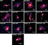 |
Fig. 1. Map of warm ionized gas traced by Hα emission from MUSE observations of our sample. |
3. Observations and data reduction
3.1. MUSE observations
We analyzed archival MUSE observations from our sample sources to measure the optical properties of the warm ionized gas. Table A.1 presents the observational properties of the MUSE data for each cluster.
MUSE is an optical integral field spectrograph mounted on the Very Large Telescope (VLT) in Chile. It has a 1′×1′ field of view with a pixel size of 0.2″, and detects wavelengths from 4750 Å to 9350 Å. All observations were conducted in wide field mode (WFM) with a spectral resolution of R = 3000. Exposure times varied by source, ranging from 2700 to 11 010 seconds.
We processed the MUSE data using MUSE pipeline version 1.6.4 and ESOREX 2.1.5, which performed standard reduction of individual exposures and combined them into a final datacube. Beyond the sky subtraction provided by ESOREX, we applied additional sky subtraction using ZAP (Zurich Atmosphere Purge; Soto et al. 2016).
We modeled the final data cube using the penalized pixel fitting PPXF method (Cappellari 2023). We modeled the stellar continuum using E-MILES libraries (Vazdekis et al. 2016). We fit the stellar and emission lines together. Each optical emission line – including the ones of [OII] λλ3726,3729, [OIII] λ4959,[OIII] λ5007, [OI] λ6300, [OI] λ6363, [NII] λ6584, [NII] λ6548, [SII] λ6716, [SII] λ6731, [NI] λ5002, [CaII] λ7291, [CaII] λ7323, Hα, Hβ, and HeII λ4686, among others – was fit with a Gaussian component. We fit the doublets, such as [NII] and [OII] with separated Gaussians and without assuming a theoretical ratio. Two Gaussians were used for some sources in the central region where the AGN is located and a broader component was found. The velocities and velocity dispersions of all emission lines were tied together to ensure a consistent kinematic solution. Figure B.1 presents an example of the best-fit of the best-fit model overlaid on the observed optical MUSE spectrum.
To correct for Galactic foreground extinction, we used the recalibration of the Schlafly & Finkbeiner (2011) dust map of the Milky Way, which is based on IRAS+COBE data Schlegel et al. (1998). We generated spatially resolved flux maps of relevant emission lines for our study, including Hα, Hβ, [OI], [SII], [NII], and [OIII] doublets and auroral lines.
We corrected for intrinsic extinction in each spaxel using the color excess E(B − V) from the gas, based on the Balmer decrement Hα/Hβ = 2.86, which corresponds to case B recombination (Osterbrock & Ferland 2006, with ne = 100 cm−3 and Te = 10 000 K). We applied the Cardelli et al. (1989) extinction curve with RV = 3.1.
3.2. Chandra X-ray observations
We used all available archival Chandra observations for each cluster, except for Abell 1795, where we selected a subset of data to maintain consistent count numbers across sources. We performed data reduction and calibration using Chandra Interactive Analysis Observations software (CIAO) 4.16 Fruscione & McDowell (2006) and Chandra Calibration Database (CALDB) 4.9.2.1. Using the chandra_repro tool in CIAO, we conducted standard calibration and data reprocessing. We then subtracted standard blank sky background files and readout artifacts. Using CIAO’s wavdetect package, we identified and removed point sources from the exposure-corrected Chandra image. Table A.1 summarizes the observational properties of the Chandra observations for each cluster.
4. Analysis
Warm-gas phase abundance measurements are highly dependent on the process that ionized the gas. The broad wavelength coverage of the MUSE spectra enables comparison of several optical emission-line diagnostics to constrain the ionization sources of the warm gas, which is necessary to determine the oxygen abundance of the warm ionized gas. The primary optical line ratios used to study the gas ionization mechanism are [NII]λ6583/Hα and [OIII]λ5007/Hβ, known as the Baldwin, Phillips, & Terlevich diagram (BPT; Baldwin et al. 1981). We also analyzed the warm ionized gas line ratios [SII]/Hα and [OI]/Hα, as these ratios are sensitive to the source of ionizing radiation.
The BPT-diagrams are useful to discriminate between the low-ionization process of the gas due to stellar photoionization (also known as star-forming HII regions) and due to harder ionizing processes such as those produced from the central AGN and fast shocks. We used the spatially resolved BPT diagram to separate the different regions; namely, the HII region, AGNs, LINERs (low-ionization nuclear emission-line regions)1 (low ionization nuclear emission) and composite regions. We caution that the classifications can be diagram-dependent; for example, a region can be classified as a LINER-like in the SII-BPT or OI-BPT but as a star formation on the NII-BPT diagram.
5. Results
5.1. Ionization mechanism of the warm gas
Before computing the O/H abundance of the warm gas, one needs to understand what is ionizing the gas in order to use a proper abundance calibrator. The BPT-diagram can be used to constrain the main source of ionizing radiation, by classifying a set of emission lines into one of four classes: (i) HII regions, (ii) Seyfert, where the ratios are consistent with ionization by an AGN, (iii) LINERs, where the ratios are consistent with multiple mechanism – photoionization by hot and evolved starts, pAGB stars, shock-excited gas, reprocessing of the EUV and soft X-ray radiation from the plasma cooling, and mixing layers, (iv) a composite of several ionization processes, such as the ones mentioned before.
For our sample, we identify three types of systems based on the BPT diagram – (i) the ones that only occupy a LINER-like emission region (Centaurus, M87, M84, and Abell 496), (ii) sources for which most of the spaxels are in the composite region (Abell 2597, PKS0745−19, Abell S1101, Abell 1835, Abell 1795, 2A0335+096, Hydra-A, and NGC5846, see Fig. 2), and (iii) sources for which most of the spaxels are in the HII region but for which some are also in the composite (RXJ0821+0752).
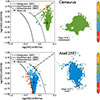 |
Fig. 2. Example of resolved BPT-NII classic diagrams for Centaurus (top panels), and Abell 2597 (bottom panels). Spaxels are color-coded based on their location relative to boundaries between the well-known empirical and theoretical classification schemes Kewley et al. (2001), Kauffmann et al. (2003), Schawinski et al. (2007) shown in solid, dashed, and pointed black lines, respectively. Yellow, green, blue, and red spaxels correspond to AGN-, LINER-, composite-, and HII-dominated regions, respectively. |
The central regions of most sources are dominated by LINER ionization (PKS0745−19, Abell S1101, 2A0335+096 in NII BPT). RXJ0821+0752 presents an interesting case: its central region shows HII-dominated ionization, while regions at greater distances exhibit composite ionization.
We find that the ionization sources in our sample have variable impacts at different radii (Lagos et al. 2022). Therefore, the determination of oxygen abundances cannot rely on the assumption of classical HII photoionization conditions throughout the interstellar medium of the galaxies.
5.2. Abundance of the warm gas
The gas-phase oxygen abundance (O/H) is a widely used and reliable tracer of metallicity in the interstellar medium of galaxies. Oxygen is one of the most abundant heavy elements, and its key ionization stages produce strong optical emission lines, making it readily accessible through spectroscopic observations. We derived the gas-phase O/H abundances using emission-line ratios from MUSE data, applying a range of calibration methods tailored to the dominant ionization mechanism in each source and region. These include: (1) the HII-region calibration from Marino et al. (2013), (2) the LINER calibration from Kumari et al. (2019), and models appropriate for composite and LINER-like ionization sources, such as (3) X-ray/EUV photoionization models from Polles et al. (2021), and (4) post-asymptotic giant branch (pAGB) star models from Rauch (2003). Additionally, we computed metallicities using the direct Te method where applicable. A detailed comparison of these methods and their associated systematics is presented in Appendix C.
5.2.1. HII ionization
For sources showing HII ionization, we derived O/H gas abundance the ratio, O3N2 = log([O III]λ5007/Hβ)− log([ NII]λ6583/Hα), calibrated by Pettini & Pagel (2004), and later refined by Marino et al. (2013).
 (1)
(1)
This calibration is valid for O3N2 values between –1.1 and 1.7, which approximately correspond to an oxygen abundance range of 12 + log(O/H) = 8.16 − 8.76.
5.2.2. Composite and LINER ionization
Two mechanisms that have been described as being potentially responsible for powering the ionization of the filaments, composite and LINER-like ionization, are the soft X-ray and EUV emitting from the cooling gas (Ferland et al. 2009; Polles et al. 2021), and pAGB stars (Binette et al. 1994; Sarzi et al. 2010; Lagos et al. 2022). In particular soft X-ray/EUV are the great interest, since the multiphase filaments observed at the center of BCGs are believed to be formed through the condensation of the hot ICM (e.g., Li et al. 2020; Voit et al. 2019; Gaspari et al. 2020).
5.2.2.1. X-ray and EUV models:
Polles et al. (2021) present predicted emission-line ratios from CLOUDY models, described as single-component plane-parallel models of constant-pressure self-irradiated clouds. In the models of Polles et al. (2021), the emission lines are photoionized by X-ray/EUV emission and can reproduce well the optical emission lines observed in cooling clusters. The models also include extra heating described with a turbulent velocity, which can be produced by, for example, AGN jets, turbulent mixing between hot and cold phases, and collisions between filaments. The models incorporate a range of metallicities (Z/Z⊙; between 0.3 and 1 Z⊙), and turbulent velocities (Between 0.0 and 100 km s−1). We derived the O/H abundance of the warm-phase gas using grids of models present in Polles et al. (2021).
Some sources in the LINER region with very high [NII]/Hα ratios, including Centaurus, M87, and A 496, could not be fit with Polles et al. (2021) models because of their high metallicity (Z > 1 Z⊙).
5.2.2.2. pAGB models:
We derived the O/H abundance using the pAGB NLTE models (Rauch 2003) implemented on the HII-CHI-mistry code for optical emission lines v.5.5 (Pérez-Montero et al. 2019). HII-CHI-Mistry, which was originally developed by Pérez-Montero (2014) for HII regions but was later extended to AGN sources (Pérez-Montero et al. 2019) and extreme emission-line galaxies (Pérez-Montero et al. 2021). HII-CHI-Mistry is Bayesian-like Python, which was originally developed by to calculate chemical abundances and physical properties using emission line fluxes from ionized gaseous nebulae. HII-CHI-Mistry employs a grid of photoionization models with three free parameters: the chemical properties of the gas-phase ISM, 12 + log(O/H) and log(N/O), and the ionization parameter log(U). These parameters are estimated from emission line ratios that are sensitive to them.
As inputs, we used the following emission lines, depending on the source, [OIII]λ4959, [OIII]λ5007, [NII]λ6584, [SII]λ6717, and [SII]λ6731, and [OII]λ7319,7330.
5.2.3. LINER ionization
For LINER-dominated regions, we used the calibration presented in Kumari et al. (2019):
 (2)
(2)
where, O3 = log([O III]λ5007/Hβ).
5.2.4. Direct Te-method
For Abell 1835 and RXJ0821+0752, we calculated the O/H abundance using the Te method (Kewley & Ellison 2008). We used the integrated [OII]λ3726 + λ3729 luminosities from Gingras et al. (2024) detected with Keck Cosmic Web Imager (KCWI). We recall that adopting a constant F([OII]λ3727)/F(Hβ) ratio results in oxygen abundance estimates with negligible variation: using F([OII]λ3727)/F(Hβ) between 0.3–0.8 yields a (O/H) difference of 0.03 dex (Lagos et al. 2014). To ensure consistency, we used the same aperture to measured [OIII]λ4959, [OIII]λ5007, and Hβ fluxes from the MUSE observations for both sources.
We derived an integrated Te and density, ne, using pyNeb (Luridiana et al. 2015), along with the [NII]λ6548, [NII]λ6584, and [NII]λ5755 auroral lines across the nebulae, and the [SII] emission lines to determine the electron density, ne. We also tried [OIII]λ4636 and [OIII]λ5007 ratios to derive the electron Te for Abell 1835. We found that [OIII] lead to higher Te compared to [NII] ratios. [OIII]λ4636 was not detected for RXJ0821+0752. This behavior has been reported in the literature (e.g., Khoram et al. 2024), where several line ratios were used to derive Te, and it appears that [OIII] is the only indicator that leads to a higher Te at higher metallicity (> 8.6) due to likely contamination from Feλ4360 or an unknown physical process (Fig. 5 of Khoram et al. 2024). We carefully checked the [OIII] auroral line, indicating contamination from Feλ4360. Due to that reason, we used the Te derived using [NII] ratio. For Abell 1835, we found a Te of 8888 ± 164. For RXJ0821+0752, we derived a Te of 8934 ± 251.
Following, we derived the oxygen abundance using the ATOM.GETIONABUNDANCE routine from pyNeb, and used the line ratios, R2 = ([OII]λ3726 + [OII]λ3729)/Hβ, and R3 = ([OIII]λ4959 + [OIII]λ5007)/Hβ, to derive  and
and  , respectively. The total O/H abundances were then derived using
 (3)
(3)
In Appendix C we present a comparison of the Te abundance measurements and alternative methods.
5.3. Abundance of the hot gas
We extracted spectra from roughly the same region as that covering the warm gas to determine the abundance of the hot gas. For some sources we used multiple regions, depending on the number of counts. The spectra were fit using XSPEC version 12.13.1 (Arnaud 1996) to derive the abundance using two apec models, which represent thermal emission of the hot ICM gas and the cooler emitted gas (phabs*(apec + apec)). The fit was restricted to 0.5–7.0 keV energy band. A blank-sky field was used to constrain the background emission. The adopted values of the Galactic column density (NH) for the galactic absorption (phas) model were obtained from the Colden (Galactic neutral hydrogen density calculator). We used the solar abundance table from Asplund et al. (2009). In Fig. B.1 we show an example of an X-ray spectrum for one region in Abell 2597 using one observation, together with the best fit model.
The abundances of the two apec models were tied together, while the temperature and the normalization were allow to vary freely. In Table 2 we list our results. For the case of NGC5846, we fixed the lower temperature to half of the higher temperature (kThigh = 0.93 ± 0.02 keV). Our results are consistent with previous works (e.g., Panagoulia et al. 2015).
Summary of metallicity measurements.
6. Discussion
This paper investigates the metallicity of both the warm and hot gas phases in massive elliptical galaxies. Because the ionization mechanism of the warm gas is uncertain, we derived gas-phase abundances using multiple approaches. For LINER-dominated regions, we applied Eq. (2) and post-AGB (pAGB) models. For HII regions, we used Eq. (1) to estimate the O/H abundance. For composite regions, we derived the O/H abundances of the warm gas using pAGB and X-ray/EUV photoionization models, which account for the composite nature of the ionization in these regions.
Subsequently, we discuss our results in the context of the AGN feedback mechanism. We then compare the warm and hot phase metallicity of our sample and examine the implications of our findings. We assume a solar O/H abundance of 8.69 from Asplund et al. (2009).
6.1. AGN feedback effect on the O/H abundance
Figures D.1 show median O/H abundance profiles of the warm gas. The resolved BPT classification, color-coded by ionization mechanism, is also shown. Additionally, we provide resolved O/H abundance maps, derived using the calibration or model appropriate for each spaxel’s ionization source. The HII calibrations presented in Sect. 5.2.1 were applied exclusively to spaxels in the outer regions of Abell 1835 and the central region of RXJ0821, where the ionization is dominated by star-forming activity.
Given the uncertainty in the dominant ionization mechanism within the composite spaxel, we derived the O/H abundance using two independent photoionization models: post-AGB and X-ray/EUV. Both models have been shown to reproduce the optical emission-line ratios observed in systems with mixed ionization (Krabbe et al. 2021; Polles et al. 2021; Lagos et al. 2022). Consequently, O/H abundances estimated from post-AGB and X-ray/EUV models are considered more robust, particularly in environments where the ionization source is ambiguous or comprises a mixture of contributors.
For LINER spaxels, we also measured the O/H abundance using two independent methods: the calibrations presented by Kumari et al. (2019, see our Sect. 5.2.3) and the post-AGB photoionization models, as they can also reproduce the LINER ionization (see Krabbe et al. 2021 and Lagos et al. 2022). For each composite or LINER spaxel, we therefore computed two separate metallicity estimates, one from each model, without selecting between them. The O/H maps derived for each sources are shown in Figs. D.1.
To construct the O/H profiles, we first computed the oxygen abundance for each spaxel using the calibration or model appropriate for its ionization mechanism (as is described above). The annuli were centered on the galaxy nucleus, and the median O/H value was calculated from all spaxels at a given radius for each O/H map separately. The shaded pink band in the profiles represents the range of O/H values obtained from the different methods, as is shown and described in Fig. C.1. This band illustrates that, while the absolute O/H values may vary slightly between methods, the overall radial trend remains unaffected by the adopted calibration.
In the same vein, the radial profiles presented in this work include both determinations for the composite and LINER spaxels, with the differences between the methods reflected in the shaded regions. We followed this approach to account for the ambiguity in identifying the dominant ionization mechanism in these regions. Both models yield similar trends in the O/H abundance profiles, with the post-AGB models giving, on average, values approximately 0.15 dex higher than those derived from the X-ray models (see Appendix C), indicating the gradient remains robust against the adopted ionization model.
The role of the ionization parameter, U, in shaping the derived metallicities deserves careful consideration. In our analysis, variations in U do not bias the metallicity estimates, particularly in the case of the pAGB models, which compare the observed emission-line ratios with grids of photoionization models to simultaneously determine (12 + log10(O/H)) and (log10U) in a nondegenerate way. In these models, U is primarily constrained by the relative strength of the [NII] lines and high-excitation coronal lines such as [NII]λ5755, both of which are sensitive to the hardness of the ionizing radiation field. The resolved maps of both quantities reveal that regions with lower O/H also exhibit lower values of log10U, consistent with more efficient cooling and softer ionizing spectra in metal-rich environments. The observed gradient in log10U supports the presence of a diluted and extended ionizing field – likely produced by pAGB or X-ray sources rather than a central AGN. Although we cannot entirely rule out that part of the O/H radial profile reflects model-dependent correlations (see Ji & Yan 2022), variations in the ionization parameter are explicitly incorporated into the abundance determinations. Consequently, differences in excitation or radiation-field hardness are intrinsically accounted for in the derived metallicities.
As is shown in Figs. D.1 some, but not all, sources in our sample exhibit clear positive O/H abundance gradients in the inner region of the gas, with O/H increasing with distance from the galaxy center. This behavior appears independently of the ionization of the source, and thus the abundance calibrator or models. The O/H abundance difference between central and outer gas regions spans from 0.1 to 0.4 Z⊙.
X-ray observations of some galaxy clusters and groups show that overall the abundance is higher at the center, and then drops to larger radii (0.1–0.3 Z⊙; e.g., Mernier et al. 2017). However, some galaxy clusters and groups show an abundance drop within 1–10 kpc in their hot gas profiles, with a peak at about 10 kpc before declining again at larger radii (e.g., Centaurus, M87, Abell 2597, Liu et al. 2019; Cavagnolo et al. 2009). These central abundance drops in the hot gas appear across several elements – particularly Fe, Si, S, Mg, O, and Ca (e.g., Churazov et al. 2003; Churazov & Inogamov 2004; Panagoulia et al. 2015; Mernier et al. 2017; Gendron-Marsolais et al. 2017; Rasmussen & Ponman 2007). These drops are more pronounced than those we observed in the warm gas phase, reaching from 0.5 Z⊙ to 2 Z⊙ in Centaurus within 10 kpc (Sanders & Fabian 2006).
One explanation for these central abundance drops is that a significant fraction of metals become deposited into dust grains and trapped in dusty filaments after cooling from the hot gas (e.g., Panagoulia et al. 2013, 2015; Liu et al. 2019). These dust grains are then displaced by buoyant bubbles and jets, and released back into the hot gas outside the core, creating O/H abundance drops. This hypothesis predicts that abundance drops should not occur for two noble gases, Ne and Ar, as they do not easily deposit into dust grains (Lakhchaura et al. 2019).
Another explanation for central abundance drops is that they are due to mechanical processes, such as the displacement of metal-rich gas from the center to larger distances by AGN-driven feedback (Liu et al. 2019). There are examples of central cluster galaxies where X-ray cavities and bubbles created by AGN feedback can lift metals in their wake. This leads to an enhanced hot gas-phase metallicity along the jet axis, compared to the perpendicular direction (Liu et al. 2019), as is also supported by hydrodynamic simulations of AGN outflows (Gaspari et al. 2011a). In the same vain, MUSE observations of the Teacup (z = 0.085) quasar also show higher O/H around the radio bubble edges, compared to rest of the nebulae, suggesting AGN feedback can produce metal enrichment at large distances (Venturi et al. 2023). Alternatively, the metals could be depleted in colder phases, such as the cold molecular gas.
The observed O/H abundance drops could also be influenced by variations in the ionization parameter, as is discussed above, as regions with higher excitation yield lower apparent abundance. While our modeling accounts for this degeneracy, we cannot fully rule out that part of the gradient arises from changes in ionization conditions.
We also note that the presence of a hidden AGN could not explain the large-scale (several kiloparsec) variations observed in the O/H abundance. Ionization from an AGN typically dominates only the innermost regions (< 1 kpc).
Overall, the variation in the abundance profile in the warm gas phase could be attributed to the contribution from these factors. This abundance drop may be closely linked to the abundance of the hot gas. It is worth mentioning that, as is shown in X-ray studies, not all clusters show a warm-phase abundance drop. In fact, many clusters are consistent with flat warm O/H abundance profiles. One explanation is that as soon as the filaments form and cool down to lower temperatures (< 10 000 K), the hot gas is being replenished by the large-scale flows.
6.2. Warm and hot gas-phase metallicity correlation
We derived the metallicity of the warm gas by converting its O/H abundance using the solar O/H abundance of 8.69 from Asplund et al. (2009), following
 (4)
(4)
Table 2 summarizes the metallicities (in solar units) for each source, measured across different regions selected based on their ionization states and using the methods described in Sect. 5.2. Specifically, since pAGB and X-ray/EUV photoionization models successfully reproduce the optical emission in most of our sources, we used these models to derive the O/H abundance in two regions: one near the center and one farther out. For sources dominated by LINER-like emission, we applied the corresponding LINER calibrations to the same two regions (e.g., Centaurus, M87). For specific regions ionized by HII, LINERs, and composite regions, we derived the O/H abundance by applying the appropriate calibrations for each ionization mechanism.
We used the abundance table from Asplund et al. (2009) to calculate the hot gas metallicity, as is detailed in Sect. 5.3. The hot gas metallicity was calculated within regions similar to those used for the warm gas. We note that this was not possible for some sources due to low counts, so we computed the hot gas metallicity using a region that covered the entire warm gas.
To explore whether the warm and hot gas phase metallicities are similar, in Fig. 3 we show the metallicity of the warm gas compared to that of the hot gas. We have also included O/H abundance measurements from a high-redshift cluster, MACS1931.8-2635 (z = 0.3525), from MUSE observations discussed in Ciocan et al. (2021).
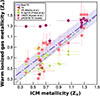 |
Fig. 3. Comparison of warm and hot-gas phase metallicities for a sample of sources using MUSE and Chandra observations. We derived the warm gas metallicity using various calibration methods, depending on the source and their ionization mechanism. For LINER-like regions and sources (magenta circles), we used the Kumari et al. (2019) calibration. For HII-dominated regions, we used the Marino et al. (2013) calibration (yellow circles). Composite and LINER region derived using pAGB models are shown with pink rectangles. The warm-phase metallicity obtained from X-ray/EUV models are shown with green crosses. Three sources, including MACS 1931.8-2635, have warm-gas metallicity measurements using the Te-direct method (red inverted triangles). The errors for the warm gas phase abundance we included both the uncertainties associated with the calibration and 1σ deviation for the regions. The dashed purple line corresponds to the best fit, and the dashed region corresponds to 1σ uncertainty. The dashed gray line shows the one-to-one relation. The best fit corresponds to |

As is shown in Fig. 3, the warm and hot gas phase metallicities show a positive correlation. We used the LINMIX Bayesian method (Kim 2017) to fit the warm–hot gas phase metallicity correlation for the sources in our sample. One of the advantages of using the Bayesian method for linear regression is that the scatter is treated as a free parameter, together with the normalization, intercept, and slope (Gaspari et al. 2019). The best-fit for the correlation is  . Each parameter corresponds to the average of the distribution with 1σ errors given by the standard deviation. The scatter corresponds to 0.06 ± 0.007, and the correlation to 0.75 ± 0.03. The Pearson (p) value of the correlation is p = 0.77. The correlation between the metallicity of both phases suggests that the gas phases are tightly coupled, and that the filaments form via turbulent condensation of the hot gas, as has been indicated by many theoretical and numerical studies (e.g., Gaspari et al. 2013; Li et al. 2015, 2020; Gaspari et al. 2017; Voit et al. 2017; Beckmann et al. 2019; Storchi-Bergmann & Schnorr-Müller 2019).
The scatter in the relation is likely driven by the different indirect methods used to measure the O/H abundance in the warm gas. In addition, the difference in metallicity between the hot and warm-gas phases can be attributed to the long mixing time, (tmix = l/vl), where l and vl are the length and turbulent velocity of the gas. For a typical cooling flow cluster, with a warm filament length of 10 kpc and velocity of 100 km s−1, the turbulent mixing time is on the order of a few 100 Myr, comparable to the cooling time. Metals produced during star formation eventually mix with the hot gas phase after a few 100 Myr, which explains the metallicity differences between the hot and warm gas phases. For chemical enrichment from type Ia supernovae, typical timescales range from ∼50 Myr for an instantaneous starburst to ∼0.3 Gyr for a typical elliptical galaxy (Matteucci & Recchi 2001).
Hydrodynamical simulations of self-regulated AGN feeding and feedback also predict a higher metallicity in the colder phase than the surrounding hot phase during the strong AGN feedback injection stage (Gaspari et al. 2011a,b), as it entrains the central metals of the BCG into the surrounding atmosphere. After the AGN jets are triggered via chaotic cold accretion (CCA), extended filamentary cool gas starts to condense from the high-metallicity outflowing parcel of hot gas. As the AGN jets shut down (due to the quenched accretion), the cool gas will detach and rain back toward the center, where it will ultimately mix with the surrounding gas via turbulent diffusion, lowering the warm gas-phase metallicity. The AGN feedback could also spread centrally enriched metals to the outskirts of galaxies, into the halo and beyond on timescales of a few hundred million years (Beckmann et al. 2019). Overall, the circulation flow driven by mechanical AGN feedback is a key mechanism to induce recursive variations in metal gradients, especially in massive central galaxies.
One of the implications of our work concerns the cold molecular gas content, as the CO-to-H2 conversion factor (αCO) heavily relies on the metallicity (Bolatto et al. 2013). All ALMA studies of massive cluster galaxies up to now (e.g., Salomé et al. 2011; Russell et al. 2019; Olivares et al. 2019) have assumed solar metallicity. We have found that the warm ionized gas, and likely the cold gas as well, shares a similar metallicity to the hot gas, which in most cases differs significantly from 1 Z⊙. The strong assumption on the metallicity can result in the understimation of the H2 mass traced by CO for some sources by almost an order of magnitude if the gas has a metallicity of 0.5 Z⊙, when a galactic αCO is considered (Amorín et al. 2016). The accurate measurement of the colder gas metallicity is crucial for addressing AGN feedback models, which report larger molecular gas masses than actual observations (e.g., Russell et al. 2019; Olivares et al. 2019).
6.3. Star formation
Central cluster galaxies show a broad range of SFRs. Studies suggest that they are correlated with their ICM properties as predicted by precipitation and CCA models (Gaspari et al. 2011a; Beckmann et al. 2019). Star formation, in turn, contributes to the ionization of the filaments, as was discussed by McDonald et al. (2011). As is shown in this study, sources located in the composite region have higher SFRs of around 10–100 M⊙ yr−1 (e.g., Abell 2597, Abell 1835, PKS0745-19, Abell 1795), while sources dominated by LINER-like emission have very low SFRs of around 1 M⊙ yr−1 (Centaurus, M87, M84, and Abell 496). This trend may be explained by the Hα being enhanced by star formation processes, which move the spaxels towards the composite or HII-dominated regions. However, measuring the SFR solely from Hα emission may lead to an overestimation of the SFR, due to the significant contribution of gas emission from composite or LINER-like regions.
6.4. Limitations
A key limitation of this work concerns the O/H abundance measurements of the warm gas. Indirect methods, primarily calibrated for HII regions, vary significantly and typically yield higher metallicity values than direct methods based on electron temperatures, Te (Kewley & Ellison 2008) – a pattern we observed in two of our systems. While the O/H abundance diagnostics we used have been calibrated for metallicities between 7.6 and 8.9, making them suitable for our systems, they were developed specifically for HII regions. This presents a challenge since our sample sources show various ionizing mechanisms, with most being composite in nature. We have tackled that by using different photoionizaiton models, such as pAGB stars and X-ray/EUV models, which can reproduce the emission line ratios of filaments.
As is discussed throughout this work, the Te-based method may provides a more accurate way to derive the gas-phase metallicity (Pilyugin 2007). Our oxygen abundance measurements using calibration based on the ionization methods may give a higher abundance compared to the Te method (see Belfiore et al. 2015 for more details). Future observations of the [OII]λλ3726,3729 lines are essential, as MUSE cannot detect these in low-redshift sources needed to have more robust O/H estimates. Using instruments such as ERIS, X-SHOOTER, or the upcoming BlueMUSE on the VLT would enable more precise warm gas abundance measurements through the “direct” Te method. Recent studies have also noted that the Te method faces challenges due to large temperature fluctuations across galaxies, which can bias metallicity estimates that are lower than true metallicities (Cameron et al. 2023). In addition, the Te mode is considered more reliable for calculating metallicity in low-metallicity environments (Pagel et al. 1992; Izotov et al. 2006), whereas in higher-metallicity environments, the Te drops, making it more difficult to detect auroral lines.
It is worth noting that the metallicity measured in the hot gas through the APEC modeling is driven by the Fe abundance, while the warm phase of the gas traces the oxygen abundance. To date, studies using various different X-ray observatories have reported a nearly solar abundance ratio of the hot gas at cluster centers, such as XMM-Newton (Mernier et al. 2018), Suzaku (Sarkar et al. 2022), and Hitomi (Hitomi Collaboration 2017), which indicate that both O and Fe abundances should be similar at the centers of clusters. A sizable uncertainty of approximately 20–30% remains, due to instrumental systematics and inaccuracies in atomic codes. Ongoing and future XRISM observations, along with laboratory atomic experiments, will help establish more robust abundance ratios at cluster centers.
7. Conclusions
In this paper we present metallicity measurements from both warm- and hot-gas phases in a sample of massive elliptical galaxies using high-resolution MUSE and Chandra observations.
-
We found that warm gas in most of the massive elliptical galaxies in our sample is ionized by a combination of different mechanisms that lead to a composite state, with a clear contribution from star formation activity. Four sources – Centaurus, M87, M84, and Abell 496, which are the lowest-redshift clusters – have the lowest SFRs (< 1 M⊙ yr−1) in the sample, and their ionized gas is dominated by LINER-like emission. The remaining sources in our sample – 2A0335, A1795, A1835, A2597, AS1101, Hydra-A, and PKS0745 – have higher SFRs (> 1–200 M⊙ yr−1) and are dominated by composite ionization. Finally, only RXJ0821+0752 is dominated by HII ionization, with some contribution from LINER-like emission in the outer regions.
-
We measured warm-gas metallicities using MUSE observations and different methods and derived hot-gas phase metallicities from Chandra observations within regions where warm ionized gas is displayed. We found that metallicities in both phases range between 0.3 Z⊙ and 1.5 Z⊙.
-
We found a positive linear correlation,
 , between the warm- and hot-gas phase metallicities, suggesting that these phases are strongly connected. The scatter corresponds to 0.06 ± 0.007 and the correlation value to 0.75 ± 0.03. The correlation suggests the warm gas originates from the thermally unstable cooling and condensation of the hot halo, which later triggers the AGN feedback.
 -
The gas metallicity profiles exhibit a central drop in some systems, peaking at a few kiloparsecs before declining at larger radii. These patterns suggest that AGN mechanical feedback may have transported metals outward – as is shown by hydrodynamical simulations – creating the central metallicity deficiency. Nevertheless, we cannot rule out the possibility that metals are partially depleted into the colder gas phase, or that the observed metallicity abundance trends could arise from variations in the ionization conditions.
Future observations from telescopes such as X-SHOOTER and the upcoming blueMUSE on the VLT will provide more precise measurements of the oxygen abundance in the warm gas phase using the direct Te method from [OII] and [OIII] emission lines – a capability that MUSE lacks for most low-redshift clusters. Additionally, X-ray observations from the newly launched XRISM satellite will deliver more accurate measurements of the hot gas metallicity and abundance for several sources discussed in this paper.
Acknowledgments
VO acknowledges support from the DICYT ESO-Chile Comite Mixto PS 1757, Fondecyt Regular 1251702. PT acknowledges support from NASA’s NNH22ZDA001N Astrophysics Data and Analysis Program under award 24-ADAP24-0011. MG acknowledges support from the ERC Consolidator Grant BlackHoleWeather (101086804). PL gratefully acknowledges support by the GEMINI ANID project No. 32240002. ET acknowledges support from ANID programs CATA-BASAL FB210003 and FONDECYT Regular grants 1241005 and 1250821. Based on observations collected at the European Organisation for Astronomical Research in the Southern Hemisphere under ESO programme(s): 094.A-0859(A), 095.B-0127(A), 60.A-9312(A), 0102.B-0048(A), 097.A-0366(A), 0103.A-0447(A), 095.B-0127(A), 097.A-0909(A).
References
- Amorín, R., Muñoz-Tuñón, C., Aguerri, J. A. L., & Planesas, P. 2016, A&A, 588, A23 [NASA ADS] [CrossRef] [EDP Sciences] [Google Scholar]
- Arnaud, K. 1996, ASP Conf. Ser., 101, 17 [NASA ADS] [Google Scholar]
- Asplund, M., Grevesse, N., Sauval, A. J., & Scott, P. 2009, ARA&A, 47, 481 [NASA ADS] [CrossRef] [Google Scholar]
- Baldwin, J. A., Phillips, M. M., & Terlevich, R. 1981, PASP, 93, 5 [Google Scholar]
- Beckmann, R. S., Dubois, Y., Guillard, P., et al. 2019, A&A, 631, A60 [EDP Sciences] [Google Scholar]
- Belfiore, F., Maiolino, R., Bundy, K., et al. 2015, MNRAS, 449, 867 [NASA ADS] [CrossRef] [Google Scholar]
- Bellstedt, S., Lidman, C., Muzzin, A., et al. 2016, MNRAS, 460, 2862 [Google Scholar]
- Binette, L., Magris, C. G., Stasińska, G., & Bruzual, A. G. 1994, A&A, 292, 13 [NASA ADS] [Google Scholar]
- Bolatto, A. D., Wolfire, M., & Leroy, A. K. 2013, ARA&A, 51, 207 [CrossRef] [Google Scholar]
- Cameron, A. J., Katz, H., & Rey, M. P. 2023, MNRAS, 522, L89 [NASA ADS] [CrossRef] [Google Scholar]
- Cappellari, M. 2023, MNRAS, 526, 3273 [NASA ADS] [CrossRef] [Google Scholar]
- Cardelli, J. A., Clayton, G. C., & Mathis, J. S. 1989, ApJ, 345, 245 [Google Scholar]
- Cavagnolo, K. W., Donahue, M., Voit, G. M., & Sun, M. 2009, ApJS, 182, 12 [Google Scholar]
- Churazov, E., & Inogamov, N. 2004, MNRAS, 350, L52 [NASA ADS] [CrossRef] [Google Scholar]
- Churazov, E., Forman, W., Jones, C., & Böhringer, H. 2003, ApJ, 590, 225 [NASA ADS] [CrossRef] [Google Scholar]
- Ciocan, B. I., Ziegler, B. L., Verdugo, M., et al. 2021, A&A, 649, A23 [NASA ADS] [CrossRef] [EDP Sciences] [Google Scholar]
- Conselice, C. J., Gallagher, J. S., III, & Wyse, R. F. G. 2001, AJ, 122, 2281 [NASA ADS] [CrossRef] [Google Scholar]
- de Plaa, J., Kaastra, J. S., Werner, N., et al. 2017, A&A, 607, A98 [NASA ADS] [CrossRef] [EDP Sciences] [Google Scholar]
- Edge, A. 2001, MNRAS, 328, 762 [NASA ADS] [CrossRef] [Google Scholar]
- Eskenasy, R., Olivares, V., Su, Y., & Li, Y. 2024, MNRAS, 527, 1317 [Google Scholar]
- Eskenasy, R., Olivares, V., & Su, Y. 2025, arXiv e-prints [arXiv:2507.03218] [Google Scholar]
- Fabian, A. 2012, ARA&A, 50, 455 [CrossRef] [Google Scholar]
- Ferland, G. J., Fabian, A. C., Hatch, N. A., et al. 2009, MNRAS, 392, 1475 [NASA ADS] [CrossRef] [Google Scholar]
- Forte, J. C., Vega, E. I., & Faifer, F. 2012, MNRAS, 421, 635 [NASA ADS] [Google Scholar]
- Fruscione, A., McDowell, Jonathan C., et al. 2006, SPIE Conf. Ser., 6270, 62701V [NASA ADS] [Google Scholar]
- Fukushima, K., Kobayashi, S. B., & Matsushita, K. 2023, ApJ, 953, 112 [NASA ADS] [CrossRef] [Google Scholar]
- Gaspari, M., Melioli, C., Brighenti, F., & D’Ercole, A. 2011a, MNRAS, 411, 349 [Google Scholar]
- Gaspari, M., Brighenti, F., D’Ercole, A., & Melioli, C. 2011b, MNRAS, 415, 1549 [NASA ADS] [CrossRef] [Google Scholar]
- Gaspari, M., Ruszkowski, M., & Oh, S. P. 2013, MNRAS, 432, 3401 [NASA ADS] [CrossRef] [Google Scholar]
- Gaspari, M., Temi, P., & Brighenti, F. 2017, MNRAS, 466, 677 [Google Scholar]
- Gaspari, M., Eckert, D., Ettori, S., et al. 2019, ApJ, 884, 169 [NASA ADS] [CrossRef] [Google Scholar]
- Gaspari, M., Tombesi, F., & Cappi, M. 2020, Nat. Astron., 4, 10 [Google Scholar]
- Gendron-Marsolais, M., Kraft, R. P., Bogdan, A., et al. 2017, ApJ, 848, 26 [NASA ADS] [CrossRef] [Google Scholar]
- Gingras, M.-J., Coil, A. L., McNamara, B. R., et al. 2024, ApJ, 977, 159 [Google Scholar]
- Gitti, M., O’Sullivan, E., Giacintucci, S., et al. 2010, ApJ, 714, 758 [Google Scholar]
- Graham, A. W., Jarrett, T. H., & Cluver, M. E. 2024, MNRAS, 527, 10059 [Google Scholar]
- Hamer, S. L., Edge, A. C., Swinbanket, A. M., et al. 2016, MNRAS, 460, 1758 [Google Scholar]
- Heckman, T. M. 1980, A&A, 500, 187 [Google Scholar]
- Hitomi Collaboration (Aharonian, F., et al.) 2017, Nature, 551, 478 [Google Scholar]
- Ho, L. C., Filippenko, A. V., & Sargent, W. L. W. 1993, ApJ, 417, 63 [NASA ADS] [CrossRef] [Google Scholar]
- Hoffer, A. S., Donahue, M., Hicks, A., & Barthelemy, R. S. 2012, ApJS, 199, 23 [NASA ADS] [CrossRef] [Google Scholar]
- Izotov, Y. I., Stasińska, G., Meynet, G., Guseva, N. G., & Thuan, T. X. 2006, A&A, 448, 955 [CrossRef] [EDP Sciences] [Google Scholar]
- Ji, X., & Yan, R. 2022, A&A, 659, A112 [NASA ADS] [CrossRef] [EDP Sciences] [Google Scholar]
- Jimenez-Gallardo, A., Massaro, F., Balmaverde, B., et al. 2021, ApJ, 912, L25 [NASA ADS] [CrossRef] [Google Scholar]
- Kauffmann, G., Heckman, T. M., Tremonti, C., et al. 2003, MNRAS, 346, 1055 [Google Scholar]
- Kewley, L. J., & Ellison, S. L. 2008, ApJ, 681, 1183 [Google Scholar]
- Kewley, L. J., Dopita, M. A., Sutherland, R. S., Heisler, C. A., & Trevena, J. 2001, ApJ, 556, 121 [Google Scholar]
- Khoram, A., Poggianti, B., Moretti, A., et al. 2024, A&A, 686, A261 [NASA ADS] [CrossRef] [EDP Sciences] [Google Scholar]
- Kim, D.-W. 2017, Galaxies, 5, 60 [Google Scholar]
- Kirkpatrick, C. C., McNamara, B. R., & Rafferty, D. A. 2009, ApJ, 697, 867 [Google Scholar]
- Krabbe, A. C., Oliveira, C. B., Zinchenko, I. A., et al. 2021, MNRAS, 505, 2087 [NASA ADS] [CrossRef] [Google Scholar]
- Kumari, N., Maiolino, R., Belfiore, F., & Curti, M. 2019, MNRAS, 485, 367 [NASA ADS] [CrossRef] [Google Scholar]
- Lagos, P., Papaderos, P., Gomes, J. M., Smith, Castelli A. V., & V., Vega L. R., 2014, A&A, 569, A110 [NASA ADS] [CrossRef] [EDP Sciences] [Google Scholar]
- Lagos, P., Loubser, S. I., Scott, T. C., et al. 2022, MNRAS, 516, 5487 [NASA ADS] [CrossRef] [Google Scholar]
- Lakhchaura, K., Mernier, F., & Werner, N. 2019, A&A, 623, A17 [NASA ADS] [CrossRef] [EDP Sciences] [Google Scholar]
- Li, Y., Bryan, G. L., Ruszkowski, M., et al. 2015, ApJ, 811, 73 [Google Scholar]
- Li, Y., Gendron-Marsolais, M.-L., Zhuravleva, I., et al. 2020, ApJ, 889, L1 [NASA ADS] [CrossRef] [Google Scholar]
- Liu, H., Pinto, C., Fabian, A. C., Russell, H. R., & Sanders, J. S. 2019, MNRAS, 485, 1757 [NASA ADS] [CrossRef] [Google Scholar]
- Loubser, S. I., Lagos, P., Babul, A., et al. 2022, MNRAS, 515, 1104 [NASA ADS] [CrossRef] [Google Scholar]
- Luridiana, V., Morisset, C., & Shaw, R. A. 2015, A&A, 573, A42 [NASA ADS] [CrossRef] [EDP Sciences] [Google Scholar]
- Marino, R. A., Rosales-Ortega, F. F., Sánchez, S. F., et al. 2013, A&A, 559, A114 [NASA ADS] [CrossRef] [EDP Sciences] [Google Scholar]
- Matteucci, F., & Recchi, S. 2001, ApJ, 558, 351 [NASA ADS] [CrossRef] [Google Scholar]
- McDonald, M., Veilleux, S., Rupke, D. S. N., & Mushotzky, R. 2010, ApJ, 721, 1262 [Google Scholar]
- McDonald, M., Veilleux, S., & Mushotzky, R. 2011, ApJ, 731, 33 [NASA ADS] [CrossRef] [Google Scholar]
- McDonald, M., Bayliss, M., Benson, B. A., et al. 2012, Nature, 488, 349 [Google Scholar]
- McNamara, B. R., Wise, M., Nulsen, P. E. J., et al. 2000, ApJ, 534, L135 [NASA ADS] [CrossRef] [Google Scholar]
- Mernier, F., de Plaa, J., Pinto, C., et al. 2016, A&A, 592, A157 [NASA ADS] [CrossRef] [EDP Sciences] [Google Scholar]
- Mernier, F., de Plaa, J., Kaastra, J. S., et al. 2017, A&A, 603, A80 [NASA ADS] [CrossRef] [EDP Sciences] [Google Scholar]
- Mernier, F., Werner, N., de Plaa, J., et al. 2018, MNRAS, 480, L95 [Google Scholar]
- Mittal, R., Whelan, J. T., & Combes, F. 2015, MNRAS, 450, 2564 [Google Scholar]
- Olivares, V., Salome, P., Combes, F., et al. 2019, A&A, 631, A22 [NASA ADS] [CrossRef] [EDP Sciences] [Google Scholar]
- Olivares, V., Su, Y., Nulsen, P., et al. 2022a, MNRAS, 516, L101 [NASA ADS] [CrossRef] [Google Scholar]
- Olivares, V., Salomé, P., Hamer, S. L., et al. 2022b, A&A, 666, A94 [NASA ADS] [CrossRef] [EDP Sciences] [Google Scholar]
- Olivares, V., Su, Y., Forman, W., et al. 2023, ApJ, 954, 56 [NASA ADS] [CrossRef] [Google Scholar]
- Olivares, V., Picquenot, A., Su, Y., et al. 2025, Nat. Astron., 9, 449 [Google Scholar]
- Osterbrock, D. E., & Ferland, G. J. 2006, Astrophysics of Gaseous Nebulae and Active Galactic Nuclei (University Science Books) [Google Scholar]
- O’Sullivan, E., Kolokythas, K., Kantharia, N. G., et al. 2018, MNRAS, 473, 5248 [CrossRef] [Google Scholar]
- Pagel, B. E. J., Simonson, E. A., Terlevich, R. J., & Edmunds, M. G. 1992, MNRAS, 255, 325 [CrossRef] [Google Scholar]
- Panagoulia, E. K., Fabian, A. C., & Sanders, J. S. 2013, MNRAS, 433, 3290 [NASA ADS] [CrossRef] [Google Scholar]
- Panagoulia, E. K., Sanders, J. S., & Fabian, A. C. 2015, MNRAS, 447, 417 [CrossRef] [Google Scholar]
- Pérez-Montero, E. 2014, MNRAS, 441, 2663 [CrossRef] [Google Scholar]
- Pérez-Montero, E., Dors, O. L., Vílchez, J. M., et al. 2019, MNRAS, 489, 2652 [CrossRef] [Google Scholar]
- Pérez-Montero, E., Amorín, R., Sánchez Almeida, J., et al. 2021, MNRAS, 504, 1237 [CrossRef] [Google Scholar]
- Pettini, M., & Pagel, B. E. J. 2004, MNRAS, 348, L59 [NASA ADS] [CrossRef] [Google Scholar]
- Pilyugin, L. S. 2007, MNRAS, 375, 685 [Google Scholar]
- Polles, F. L., Salomé, P., Guillard, P., et al. 2021, A&A, 651, A13 [NASA ADS] [CrossRef] [EDP Sciences] [Google Scholar]
- Rasmussen, J., & Ponman, T. J. 2007, MNRAS, 380, 1554 [CrossRef] [Google Scholar]
- Rauch, T. 2003, A&A, 403, 709 [NASA ADS] [CrossRef] [EDP Sciences] [Google Scholar]
- Russell, H. R., McNamara, B. R., Fabian, A. C., et al. 2019, MNRAS, 490, 3025 [Google Scholar]
- Salomé, P., & Combes, F. 2003, A&A, 412, 657 [NASA ADS] [CrossRef] [EDP Sciences] [Google Scholar]
- Salomé, P., Combes, F., Revaz, Y., et al. 2011, A&A, 531, A85 [NASA ADS] [CrossRef] [EDP Sciences] [Google Scholar]
- Sanders, J. S., & Fabian, A. C. 2006, MNRAS, 371, 1483 [Google Scholar]
- Sarkar, A., Su, Y., Truong, N., et al. 2022, MNRAS, 516, 3068 [NASA ADS] [CrossRef] [Google Scholar]
- Sarzi, M., Shields, J. C., Schawinski, K., et al. 2010, MNRAS, 402, 2187 [Google Scholar]
- Schawinski, K., Thomas, D., Sarzi, M., et al. 2007, MNRAS, 382, 1415 [Google Scholar]
- Schlafly, E. F., & Finkbeiner, D. P. 2011, ApJ, 737, 103 [Google Scholar]
- Schlegel, D. J., Finkbeiner, D. P., & Davis, M. 1998, ApJ, 500, 525 [Google Scholar]
- Soto, K. T., Lilly, S. J., Bacon, R., Richard, J., & Conseil, S. 2016, MNRAS, 458, 3210 [Google Scholar]
- Storchi-Bergmann, T., & Schnorr-Müller, A. 2019, Nat. Astron., 3, 48 [Google Scholar]
- Su, Y., & Irwin, J. A. 2013, ApJ, 766, 61 [Google Scholar]
- Tamhane, P. D., McNamara, B. R., Russell, H. R., et al. 2023, MNRAS, 519, 3338 [NASA ADS] [CrossRef] [Google Scholar]
- Temi, P., Amblard, A., Gitti, M., et al. 2018, ApJ, 858, 17 [NASA ADS] [CrossRef] [Google Scholar]
- Tremblay, G. R., O’Dea, C. P., Baum, S. A., et al. 2015, MNRAS, 451, 3768 [Google Scholar]
- Tremblay, G. R., Combes, F., Oonk, J. B. R., et al. 2018, ApJ, 65, 13 [Google Scholar]
- Ubertosi, F., Gitti, M., Brighenti, F., et al. 2023, A&A, 673, A52 [NASA ADS] [CrossRef] [EDP Sciences] [Google Scholar]
- Ubertosi, F., Giacintucci, S., Clarke, T., et al. 2024, A&A, 691, A294 [NASA ADS] [CrossRef] [EDP Sciences] [Google Scholar]
- Vantyghem, A. N., McNamara, B. R., Russell, H. R., et al. 2019, ApJ, 870, 57 [NASA ADS] [CrossRef] [Google Scholar]
- Vazdekis, A., Koleva, M., Ricciardelli, E., Röck, B., & Falcón-Barroso, J. 2016, MNRAS, 463, 3409 [Google Scholar]
- Venturi, G., Treister, E., Finlez, C., et al. 2023, A&A, 678, A127 [NASA ADS] [CrossRef] [EDP Sciences] [Google Scholar]
- Vigneron, B., Hlavacek-Larrondo, J., Rhea, C. L., et al. 2024, ApJ, 962, 96 [NASA ADS] [CrossRef] [Google Scholar]
- Voit, G. M., Meece, G., Li, Y., et al. 2017, ApJ, 845, 80 [Google Scholar]
- Voit, M., Babul, A., Babyk, I., et al. 2019, BAAS, 51, 405 [Google Scholar]
Note that the LINER term is not appropriate in this context since LINERs was originally defined as being “nuclear” emission (Heckman 1980; Ho et al. 1993); alternately, LIER (low ionization emission-line region) has been suggested by recent authors.
Appendix A: Summary of the observations
Chandra and MUSE observations used in this paper.
Appendix B: Example spectra
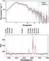 |
Fig. B.1. Top: Example X-ray spectrum of Abell 2597 from one of the two regions used to derive the hot gas-phase metallicity. The observed spectrum, corresponding to one Chandra observation, is shown as gray data points, while the best-fit model is overlaid in pink. Bottom: Example of MUSE spectrum of one spaxel of Abell 2597 shown in gray, and the best fit model is shown in pink. |
Appendix C: Warm-phase abundance comparison
In this section we compare different methods for measuring warm-gas abundance. Figure C.1 shows the comparison of O/H abundance profiles derived from X-ray, pAGB models, and HII calibration for RXJ0821. The median O/H profile is indicated by the pink line. O/H abundances derived from composite and LIN(E)R spaxels using the X-ray and pAGB models are shown as blue and black points, respectively, while values obtained from HII spaxels are shown as gray points. On average, the pAGB model yields O/H abundances that are 0.15 dex higher than those from the X-ray model, although both models exhibit a consistent radial trend across the galaxy. This behavior, systematically higher pAGB abundances while following the same radial profile, is observed for all sources in our sample.
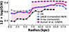 |
Fig. C.1. Comparison of O/H abundance profiles derived from the different O/H maps: X-ray/EUV and pAGB models, and HII and LINER calibration for RXJ0821. The median O/H profile is indicated by the pink line. O/H abundances profile derived from composite and LIN(E)R spaxels using X-ray and pAGB models, and LINER calibration are shown as blue, black, and purple points, respectively, while values obtained from H II spaxels are shown as gray points. |
In Fig. C.2 we plot the warm-phase metallicity distribution for different methods to showcase their measurement ranges. This plot includes measurement from different regions of the gas.
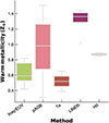 |
Fig. C.2. Diagram showing the metallicity ranges found in our sample using different methods throughout the paper. The green bar represents metallicity from X-ray/EUV models. Note that the X-ray/EUV method is limited to metallicities below 1 Z⊙. The pink bar shows pAGB stars results, the red bar indicates Te metallicities. The magenta bar shows LINER O3N2 measurements, while the gray bar correspond to results from HII O3N2 calibration. |
The LINER calibration by Kumari et al. (2019) provided the highest O/H abundance values, with measurements ranging between 1.0 and 1.4 Z⊙, with the exception of the clusters that show clear AGN ionization sources at the center.
For HII regions, the O3N2 calibration proposed by Marino et al. (2013) yielded O/H abundances between 0.85 and 0.89 Z⊙. The X-ray/EUV models showed abundances ranging from 0.4 to 0.8 Z⊙. However, these models cannot account for metallicities above 1.0 Z⊙, making it impossible to measure several high-metallicity systems such as Centaurus, M87, M84, and A496. The emission line ratios of these sources consistently indicate metallicities > 1 Z⊙.
The pAGB models yielded O/H abundances between 0.3 and 1.5 Z⊙, similar to the X-ray/EUV models but systematically higher by a median of 0.20 Z⊙.
Using the Te method, we found relatively low O/H abundances of 0.5–0.3 Z⊙ for two sources that have [OII] emission lines. In Fig. C.3, we compare the differences between X-ray/EUV measurements, pAGB models. For consistency, we computed the abundance using the integrated values the two sources following the methods described in the Sect. 5.2. The metallicity derived from Te measurements shows the closest agreement with X-ray/EUV derived metallicities, having differences of 0.1–0.17 Z⊙, and the pAGB models with 0.13–0.18 Z⊙.
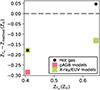 |
Fig. C.3. Comparison of the Te abundance measurements with alternative methods. The plot shows the difference between metallicities obtained with Te and other methods versus the Te-derived metallicity for two sources. Green represent metallicities derived from X-ray/EUV models, while pink squares correspond to values derived assuming photoionization by post-AGB stars. Black dots corresponds to the metallicity of the hot gas. |
Appendix D: BPT diagrams and O/H abundance maps and profiles
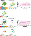 |
Fig. D.1. Examples of O/H abundance profiles from our sample, illustrating both cases where central O/H drops are detected (e.g., Centaurus, RXJ0821+0752). Upper left panel: Spatially resolved BPT diagram showing regions classified as AGN (yellow), LINER (green), composite (blue), and HII (red). The gray circles indicate the annulus used to derive O/H abundances. Upper middle panel: O/H abundance map derived using the LINER calibration for the LINER spaxels. Upper right panel: Median radial profile of the warm gas O/H abundance, computed using calibrations and models appropriate for each spaxel depending on the ionization mechanism. The shaded region shows the 85% confidence interval, estimated via bootstrapping, and reflects the range of O/H values obtained from the different methods. Bottom left, middle, and right panels: O/H abundance maps derived using the X-ray/EUV and pAGB models for the composite and LINER ionization, respectively. O/H abundance maps derived using HII calibration for the SF dominated spaxels (if applies). The pink cross shows the center of the galaxy. |
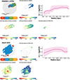 |
Fig. D.1. Continued |
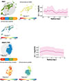 |
Fig. D.1. Continued. |
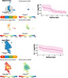 |
Fig. D.1. Continued. |
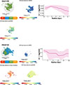 |
Fig. D.1. Continued. |
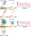 |
Fig. D.1. Continued. |
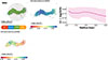 |
Fig. D.1. Continued. |
All Tables
All Figures
|
Fig. 1. Map of warm ionized gas traced by Hα emission from MUSE observations of our sample. |
| In the text | |
|
Fig. 2. Example of resolved BPT-NII classic diagrams for Centaurus (top panels), and Abell 2597 (bottom panels). Spaxels are color-coded based on their location relative to boundaries between the well-known empirical and theoretical classification schemes Kewley et al. (2001), Kauffmann et al. (2003), Schawinski et al. (2007) shown in solid, dashed, and pointed black lines, respectively. Yellow, green, blue, and red spaxels correspond to AGN-, LINER-, composite-, and HII-dominated regions, respectively. |
| In the text | |
|
Fig. 3. Comparison of warm and hot-gas phase metallicities for a sample of sources using MUSE and Chandra observations. We derived the warm gas metallicity using various calibration methods, depending on the source and their ionization mechanism. For LINER-like regions and sources (magenta circles), we used the Kumari et al. (2019) calibration. For HII-dominated regions, we used the Marino et al. (2013) calibration (yellow circles). Composite and LINER region derived using pAGB models are shown with pink rectangles. The warm-phase metallicity obtained from X-ray/EUV models are shown with green crosses. Three sources, including MACS 1931.8-2635, have warm-gas metallicity measurements using the Te-direct method (red inverted triangles). The errors for the warm gas phase abundance we included both the uncertainties associated with the calibration and 1σ deviation for the regions. The dashed purple line corresponds to the best fit, and the dashed region corresponds to 1σ uncertainty. The dashed gray line shows the one-to-one relation. The best fit corresponds to |
| In the text | |
|
Fig. B.1. Top: Example X-ray spectrum of Abell 2597 from one of the two regions used to derive the hot gas-phase metallicity. The observed spectrum, corresponding to one Chandra observation, is shown as gray data points, while the best-fit model is overlaid in pink. Bottom: Example of MUSE spectrum of one spaxel of Abell 2597 shown in gray, and the best fit model is shown in pink. |
| In the text | |
|
Fig. C.1. Comparison of O/H abundance profiles derived from the different O/H maps: X-ray/EUV and pAGB models, and HII and LINER calibration for RXJ0821. The median O/H profile is indicated by the pink line. O/H abundances profile derived from composite and LIN(E)R spaxels using X-ray and pAGB models, and LINER calibration are shown as blue, black, and purple points, respectively, while values obtained from H II spaxels are shown as gray points. |
| In the text | |
|
Fig. C.2. Diagram showing the metallicity ranges found in our sample using different methods throughout the paper. The green bar represents metallicity from X-ray/EUV models. Note that the X-ray/EUV method is limited to metallicities below 1 Z⊙. The pink bar shows pAGB stars results, the red bar indicates Te metallicities. The magenta bar shows LINER O3N2 measurements, while the gray bar correspond to results from HII O3N2 calibration. |
| In the text | |
|
Fig. C.3. Comparison of the Te abundance measurements with alternative methods. The plot shows the difference between metallicities obtained with Te and other methods versus the Te-derived metallicity for two sources. Green represent metallicities derived from X-ray/EUV models, while pink squares correspond to values derived assuming photoionization by post-AGB stars. Black dots corresponds to the metallicity of the hot gas. |
| In the text | |
|
Fig. D.1. Examples of O/H abundance profiles from our sample, illustrating both cases where central O/H drops are detected (e.g., Centaurus, RXJ0821+0752). Upper left panel: Spatially resolved BPT diagram showing regions classified as AGN (yellow), LINER (green), composite (blue), and HII (red). The gray circles indicate the annulus used to derive O/H abundances. Upper middle panel: O/H abundance map derived using the LINER calibration for the LINER spaxels. Upper right panel: Median radial profile of the warm gas O/H abundance, computed using calibrations and models appropriate for each spaxel depending on the ionization mechanism. The shaded region shows the 85% confidence interval, estimated via bootstrapping, and reflects the range of O/H values obtained from the different methods. Bottom left, middle, and right panels: O/H abundance maps derived using the X-ray/EUV and pAGB models for the composite and LINER ionization, respectively. O/H abundance maps derived using HII calibration for the SF dominated spaxels (if applies). The pink cross shows the center of the galaxy. |
| In the text | |
|
Fig. D.1. Continued |
| In the text | |
|
Fig. D.1. Continued. |
| In the text | |
|
Fig. D.1. Continued. |
| In the text | |
|
Fig. D.1. Continued. |
| In the text | |
|
Fig. D.1. Continued. |
| In the text | |
|
Fig. D.1. Continued. |
| In the text | |
Current usage metrics show cumulative count of Article Views (full-text article views including HTML views, PDF and ePub downloads, according to the available data) and Abstracts Views on Vision4Press platform.
Data correspond to usage on the plateform after 2015. The current usage metrics is available 48-96 hours after online publication and is updated daily on week days.
Initial download of the metrics may take a while.