© The Authors 2026

1 Introduction

Planetary orbits within a system are traditionally expected to be coplanar and closely aligned with their host stars’ spin axes, as they are believed to have formed from the same protoplanetary disk. This assumption is supported by the fact that in the Solar System, the Sun’s obliquity is only about 7°. However, observations of exoplanets reveal a wide range of stellar obliquities, with spin-orbit angles varying from 0 to nearly 180° (Winn et al. 2010). These obliquities, primarily measured using techniques such as the Rossiter-McLaughlin effect (Rossiter 1924; McLaughlin 1924), provide crucial insights into the diverse evolutionary histories of planetary systems.

The vast majority of stellar obliquity measurements have focused on close-in giant planets, particularly hot Jupiters (HJs). These observations commonly reveal significant spin-orbit misalignments in systems with HJs orbiting hot stars. Such misalignments have typically been interpreted as the natural outcomes of the formation of HJs through high-eccentricity migration processes. During these processes, giant planets originally located at large orbital distances are driven into highly eccentric orbits, which then evolve into tighter, tidally locked orbits through tidal interactions. The initial orbital excitations are believed to be triggered by a variety of dynamical processes, including the von Zeipel–Lidov–Kozai (ZLK) mechanism (Wu & Murray 2003; Fabrycky & Tremaine 2007; Naoz et al. 2011), secular interactions (Wu & Lithwick 2011), and planet-planet scattering (Ford & Rasio 2008; Nagasawa et al. 2008; Beaugé & Nesvornỳ 2012).

However, recent findings have shown that relying on these traditional mechanisms as the predominant pathways for HJ formulation is problematic for several reasons: (1) The occurrence rate of initially highly inclined outer massive companions, necessary to trigger the ZLK effect, is inefficient to produce the observed HJ population. (2) The scarcity of proto-HJs found on highly eccentric orbits challenges the high-eccentricity migration hypothesis (Dawson et al. 2014). (3) The isotropic distribution of stellar obliquities for misaligned HJs, revealed via a hierarchical Bayesian analysis (Dong & Foreman-Mackey 2023), disfavors the mechanisms that would result in a specific distribution.

Alternative HJ formation channels involve more quiescent processes, such as in situ formation and disk migration, which typically result in closely aligned HJs. However, to account for the high stellar obliquities observed, these mechanisms require the consideration of additional factors, notably the primordial misalignment between the protoplanetary disk and the host star’s spin axis (Batygin 2012). Furthermore, the recently proposed coplanar high-eccentricity migration pathway, which has been suggested as a likely dominant formation mechanism for HJs based on an analysis of their giant companions, also requires primordial origins for the observed obliquity distribution (Zink & Howard 2023). Therefore, it appears that primordial misalignments played a significant role in shaping the orbital configurations of HJs.

In addition to these indirect arguments, direct observations provide compelling evidence of disk misalignment. Approximately 33% (5 out of 15) of observed protoplanetary disks show misalignment with their host pre-main-sequence stars (Davies 2019), while about 19% (6 out of 31) of debris disks exhibit similar misalignments (Hurt & MacGregor 2023). A recent study also revealed a large misalignment in the protoplanetary disk around a young star (Barber et al. 2024), and observations of circular binary protoplanetary disks in polar configurations further underscore these findings (Kennedy et al. 2019). Although the samples are limited—partly due to the challenges in resolving stellar orientations in the presence of protoplanetary disks—the existing observations suggest that a moderate proportion of these disks could be significantly misaligned.

Theoretically, primordial misalignments can be generated through several mechanisms. Chaotic accretion, characterized by irregular material inflow, typically results in misalignments of up to 20° (Bate et al. 2010; Fielding et al. 2015). Magnetic warping, driven by interactions between the disk’s magnetic field and the star, leads to moderate misalignments (Lai et al. 2011; Foucart & Lai 2011). Gravitational torques from a distant inclined stellar companion, on the other hand, can produce a broad range of stellar obliquities, typically spanning from 60° to 180° (Batygin 2012; Spalding & Batygin 2015; Zanazzi & Lai 2018). Despite these well-studied mechanisms, it remains uncertain which process—or combination thereof—primarily accounts for the star-disk misalignments observed in practice.

Several recent studies have invoked these primordial misalignments to explain unique orbital configurations in multi-planet systems. For instance, the K2-290A system, which features two coplanar planets on retrograde orbits with a stellar obliquity of ψ_⋆ = 124° ± 6°, is proposed to have originated from a primordial disk misalignment driven by its stellar companion, K2-290B (Hjorth et al. 2021). Similarly, the near-perpendicular (likely retrograde) inner-outer orbits of HD 3167 have been attributed to dynamical evolution driven by a polar misaligned disk (Fu & Wang 2024). The predominantly low obliquities in Kepler’s compact multi-planet systems may reflect bifurcated evolutionary pathways driven by misaligned disks, if such primordial misalignments are common (Fu et al. 2025). Furthermore, combining high-eccentricity migration with primordial disk misalignments can reproduce a distinct population of HJs on perpendicular orbits (Vick et al. 2023).

Critically, the dynamical bifurcation-induced effect discovered by Fu & Wang (2024)—a saddle-center bifurcation during disk dispersal that induces separatrix-crossing behaviors and thus large-amplitude orbital librations—may have broadly influenced early dynamical evolution in systems with misaligned protoplanetary disks, thereby sculpting their architectures. While several previous studies have explored the early dynamics of planetary systems taking planet-disk interactions into account, they typically assume that the inner region of the disk has already dissipated (Petrovich et al. 2020; Millholland & Batygin 2019; Su & Lai 2020), or they employ a simplified gravitational model of the disk that is only valid when planets lie within the disk plane (Spalding & Millholland 2020; Zanazzi & Lai 2018). In the former case, the secular effect of the outer disk’s gravity resembles that of an external perturbing body, with its strength decaying as the disk disperses. In the latter case, Spalding & Millholland (2020) adopted a linear gravitational model of the disk that describes a constant orbit precession. In contrast, Fu & Wang (2024) and Fu et al. (2025) applied a full-space disk model that captures nonlinear gravitational effects, enabling identification of dynamical bifurcations.

In this paper, we demonstrate that the equilibrium bifurcations arise from the sin⁻¹ I dependence of the disk-induced nodal regression for orbits inclined to the disk plane. Conversely, the linear gravity model—valid only for orbits lying within the disk plane and assuming constant nodal regression—obscures this effect and predicts a qualitatively distinct dynamical evolution. Then, we systematically analyze equilibrium stability under the full-space disk gravity model and examine how perturbations from additional planets in hierarchical and compact systems modify these dynamics.

Our study does not address the formation channels of primordial misalignments (e.g., chaotic accretion, magnetic warping, or binary torques). Instead, we focus exclusively on the planetary dynamics following their establishment.

This paper is structured as follows: Section 2 presents the secular dynamical model. Section 3 details the origin of equilibrium bifurcations and their stability in a simplified system. Section 4 extends the analysis to hierarchical three-body systems. Section 5 examines compact multi-planet systems with low-mass planets. We conclude with a discussion and summary in Section 6.

2 Secular dynamical model

We considered a multi-planet system featuring a fast-rotating host star (orientation along ${\hat{\mathit{s}}}_{\star }$) and a misaligned protoplanetary disk (orientation along ${\hat{\mathit{l}}}_{\mathrm{d}}$), as shown in Fig. 1. Here we use a two-planet system with planetary masses m₁ and m₂ and semimajor axes a₁ and a₂ (a₁ < a₂) as an example. The Hamiltonian function incorporates the stellar oblateness, the disk’s gravity, and the gravitational interactions between the planets, all of which govern the planetary orbital evolution; it is presented in (Fu & Wang 2024; Fu et al. 2025) $$\begin{array}{rl}\mathcal{H}& =\sum _{i=1,2}{\mathcal{H}}_{\mathrm{k},i}+{\mathrm{\Phi }}_{\star ,i}+{\mathrm{\Phi }}_{\mathrm{d},i}+{\mathrm{\Phi }}_{12}\\ & =\sum _{i=1,2}-\frac{G{m}_i{m}_{\star }}{2a_i}+\frac{{\varphi }_{\star ,i}}{6{(1-e_i^2)}^{3/2}}[1-3{({\hat{\mathit{s}}}_{\star }\cdot {\hat{\mathit{l}}}_i)}^2]\\ & +{\varphi }_{\mathrm{d},i}\{\frac{\pi }{8}{e}_i^2+\frac{\sqrt{1-e_i^2}}{S_i}[S_i^2+\frac{e_i^2}{2}{({\hat{\mathit{l}}}_{\mathrm{d}}\cdot {\hat{\mathit{e}}}_i)}^2]\\ & -\frac{\pi }{32}[(4-3e_i^2)S_i^2+6e_i^2{({\hat{\mathit{l}}}_{\mathrm{d}}\cdot {\hat{\mathit{e}}}_i)}^2]\}\\ & +\frac{{\varphi }_{12}}{2}[5{({\mathit{e}}_1\cdot {\hat{\mathit{l}}}_2)}^2-{({\mathit{l}}_1\cdot {\hat{\mathit{l}}}_2)}^2+1/3-2e_1^2],\end{array}$$(1)

where ℋ_k,i represents the Keplerian part for planet i that does not contribute to the secular evolution, Φ_⋆,i arises from the stellar oblateness, Φ_d,i arises from the disk’s gravity, and Φ₁₂ arises from the mutual gravitational interactions between the two planets. These perturbing potentials are formed in terms of the vectorial elements, the eccentricity vector ${\mathit{e}}_i=e_i{\hat{\mathit{e}}}_i$ and the normalized orbit angular momentum ${\mathit{l}}_i=\sqrt{1-e_i^2}{\hat{\mathit{l}}}_i$. In Eq. (1), $${\varphi }_{\star ,i}=\frac{3G{m}_{\star }{m}_i{J}_2{R}_{\star }^2}{2a_i^3},$$(2) $${\varphi }_{\mathrm{d},i}=2\pi m_{i}G{\mathrm{\Sigma }}_0{a}_0,$$(3) $${\varphi }_{12}=\frac{3G{m}_1{m}_2{a}_1^2}{4a_2^3{(1-e_2^2)}^{3/2}},$$(4)

and $$S_i=\sqrt{1-{({\hat{\mathit{l}}}_{\mathrm{d}}\cdot {\hat{\mathit{l}}}_i)}^2}=\sin {\mathit{l}}_i.$$(5)

where G is the gravitational constant, m_⋆ and R_⋆ are the mass and radius of the central star, J₂ is its second zonal gravity coefficient, Σ₀ is the disk surface density at radius a₀, and I_i is the orbit inclination relative to the disk plane.

The equations of motion in terms of l and e can be obtained by substituting the Hamiltonian (Eq. (1)) into the Lagrange planetary equations (Wang & Fu 2020): $$\frac{\mathrm{d}{\mathit{l}}_i}{\mathrm{d}t}=-\frac{1}{L_i}({\mathit{l}}_i\times {\mathrm{\nabla }}_{l_i}\mathrm{\Phi }+\mathit{e}\times {\mathrm{\nabla }}_{e_i}\mathrm{\Phi }),$$(6) $$\frac{\mathrm{d}{\mathit{e}}_i}{\mathrm{d}t}=-\frac{1}{L_i}({\mathit{e}}_i\times {\mathrm{\nabla }}_{l_i}\mathrm{\Phi }+{\mathit{l}}_i\times {\mathrm{\nabla }}_{{\mathit{e}}_i}\mathrm{\Phi }),$$(7)

where $L_i=m_i\sqrt{G{m}_{\star }{a}_i}$ is the magnitude of the orbital angular momentum.

In Eq. (1), the planetary interaction potential (Φ₁₂) is derived via multipole expansion, which assumes a hierarchical orbital configuration (i.e., a₁ ≪ a₂). However, if the orbits are compact, this approximation becomes inadequate. Instead, the interaction potential can be modeled through the Laplace-Lagrange theory by assuming small eccentricities and inclinations. The lowest-order secular potential is given by $${\mathrm{\Phi }}_{12}^{\mathrm{\prime }}=-\frac{{\varphi }_{12}^{\mathrm{\prime }}}{2}{({\hat{\mathit{l}}}_1\cdot {\hat{\mathit{l}}}_2)}^2,$$(8)

where $${\varphi }_{12}^{\mathrm{\prime }}=\frac{G{m}_1{m}_2{a}_1}{4a_2^2}{b}_{3/2}^{(1)}\left(\frac{a_1}{a_2}\right).$$(9)

Here, $b_{3/2}^{(1)}(\alpha )$ is the Laplace coefficient, given by $$b_{3/2}^{(1)}(\alpha )=\frac{1}{\pi }{\int }_0^{2\pi }\frac{\cos \theta }{{(1-2\alpha \cos \theta +{\alpha }^2)}^{3/2}}\mathrm{d}\theta .$$(10)

In order to describe the gravity of the disk over the entire space, we derived the secular potential of the disk (Φ_d,i) in Eq. (1) using the thin disk model (Cuddeford 1993; Schulz 2012). To further analyze how the disk’s gravity drives precession in a planetary orbit, we considered the case of a circular orbit (e = 0). By substituting Φ_d,i from Eq. (1) into Eq. (6) with e_i = 0, we obtain $$\dot{\mathrm{\Omega }}\approx -\frac{2\pi G{\mathrm{\Sigma }}_{\mathrm{a}}}{na(\sin I+\beta )}$$(11)

where β is the softening parameter, and I and Ω are the planet’s inclination and longitude of the ascending node relative to the disk plane, respectively. This result is consistent with the well-known result that the nodal precession has a I⁻¹ dependence of the leading term (Ward 1981). Given this explicit inclination dependence, we refer to this as the nonlinear model.

In contrast, several previous studies have adopted a thick-disk model – derived by using Laplace-Lagrange theory – to describe the disk’s gravity near the disk plane. This model predicts a constant nodal precession rate, given by $$\dot{\mathrm{\Omega }}\simeq -\frac{\pi G{\mathrm{\Sigma }}_a}{nah},$$(12)

where h is the disk aspect ratio h = H/r (H is the disk scale height). This version of the disk model is valid only when the planet lies within the disk plane, i.e., $|{\hat{\mathit{l}}}_i\times {\hat{\mathit{l}}}_{\mathrm{d}}|\ll h\ll 1$ (Ward 1981; Zanazzi & Lai 2018). Since Eq. (12) results from a linearized treatment of the perturbing potential, we refer to this as the linear model.

In summary, Eq. (11) follows from the thin-disk gravitational potential (Φ_d,i) in Eq. (1), which is valid across the physical domain. Equation (12), on the other hand, is based on a thick-disk potential that has been linearized under the assumption of small inclinations. We find that when the softening scale is set to β = h and the inclination I is small, the precession rate from the thin-disk model (Eq. (11)) closely matches that of the thick-disk model (Eq. (12)). This indicates that the thin-disk approximation with appropriate softening provides a reasonable description of gravitational effects across the entire spatial domain – even for planets near the disk plane. Conversely, applying the linearized model (Eq. (12)) to inclined orbits fails to accurately capture the secular evolution, as it neglects the critical nonlinear factor sin⁻¹ I, as will be demonstrated in the following section.

The surface density of the disk is assumed to follow a Mestel disk profile (Mestel 1963): $$\mathrm{\Sigma }(r)={\mathrm{\Sigma }}_0\frac{r_0}{r},$$(13)

where Σ(r) is the disk’s surface density at radius r. The disk’s mass is then $$m_{\mathrm{d}}={\int }_{r_{\text{in}}}^{r_{\text{out}}}2\pi r\mathrm{\Sigma }(r)\mathrm{d}r\simeq 2\pi {\mathrm{\Sigma }}_{\text{out}}{r}_{\text{out}}^2,$$(14)

where r_in and r_out are the inner and outer truncation radii of the disk, assuming r_in ≪ r_out.

If the disk evolves homogeneously as assumed in many previous studies (Batygin & Adams 2013; Lai 2014), the surface density, Σ(r, t), evolves in time according to $$\mathrm{\Sigma }(r,t)=\frac{{\mathrm{\Sigma }}_r(0)}{{(1+t/{\tau }_{\mathrm{d}})}^{3/2}},$$(15)

where τ_d is the timescale of the disk’s dissipation. However, realistic protoplanetary disks can evolve in a nonhomologous way due to photoevaporation. After the characteristic time τ_w, when the photo-evaporative mass-loss rate becomes comparable to viscous accretion rate at the critical photoevaporation radius r_c, photoevaporation starves the inner region of the disk (r < r_c) from resupply by the outer disk’s viscous evolution (Alexander et al. 2006, 2014; Zanazzi & Lai 2018). This leads to a rapid dissipation of the inner disk over a timescale τ_v,in ≪ τ_d, while the outer disk continues to evolve over τ_v,out = τ_d.

Assuming both the inner and outer disks follow a Mestel disk’s profile, the disk’s surface density evolution can be parameterized by (Zanazzi & Lai 2018) $$\mathrm{\Sigma }(r,t)=\{\begin{array}{ll}{\mathrm{\Sigma }}_{\mathrm{c}}(t)\left(r_{\mathrm{c}}/r\right)& r_{\text{in\hspace{0.17em}}}<r<r_{\mathrm{c}}\\ {\mathrm{\Sigma }}_{\text{out\hspace{0.17em}}}(t)\left(r_{\text{out\hspace{0.17em}}}/r\right)& r_{\mathrm{c}}<r<r_{\text{out\hspace{0.17em}}},\end{array}$$(16)

where $$\{\begin{array}{l}{\mathrm{\Sigma }}_{\mathrm{c}}(t)={\mathrm{\Sigma }}_{\mathrm{c}}(0)/{(1+t/{\tau }_{\mathrm{v},\text{in}})}^{3/2}\\ {\mathrm{\Sigma }}_{\text{out}}(t)={\mathrm{\Sigma }}_{\text{out\hspace{0.17em}}}(0)/{(1+t/{\tau }_{\mathrm{v},\text{out}})}^{3/2}.\end{array}$$(17)

Owing to their distinct surface density profiles, the gravitational fields of the inner and outer disks must be computed separately.

In this study, we assumed that orbits lie within the inner region of the disk with r_in ≪ r ≪ r_c. As a result, the potential of the inner disk has the same form as the expression Φ_d,i given in Eq. (1). The potential of the outer disk resembles that of an outer distant perturbing body (Zanazzi & Lai 2018; Fu & Wang 2024): $${\mathrm{\Phi }}_{\mathrm{d}\mathrm{o}\mathrm{u}\mathrm{t},i}=\frac{{\varphi }_{\mathrm{d}\mathrm{o}\mathrm{u}\mathrm{t},\mathrm{i}}}{2}[5{({\mathit{e}}_i\cdot {\hat{\mathit{l}}}_{\mathrm{d}})}^2-{({\mathit{l}}_i\cdot {\hat{\mathit{l}}}_{\mathrm{d}})}^2+1/3-2e_i^2],$$(18)

where $${\varphi }_{\mathrm{d}\mathrm{o}\mathrm{u}\mathrm{t},i}=\frac{3\pi G{m}_i{\mathrm{\Sigma }}_{\mathrm{o}\mathrm{u}\mathrm{t}}{r}_{\mathrm{o}\mathrm{u}\mathrm{t}}{a}_i^2}{4r_{\mathrm{c}}^2}.$$(19)

Adding this potential to Eq. (1), the contribution of the outer disk can be included. However, for r ≪ r_c, the perturbation from the outer disk becomes negligible compared to those from stellar oblateness and the inner disk. We therefore neglected this term in our initial analysis.

Fig. 1 Geometric illustration of a multi-planet system with a misaligned protoplanetary disk. The disk’s angular momentum orientation is denoted by the unit vector ${\hat{\mathit{l}}}_{\mathrm{d}}$. The host star rotates at angular velocity Ω⋆ with its spin oriented along ${\hat{\mathit{s}}}_{\star }$. The primordial stellar obliquity (ψ⋆0) corresponds to the angle between ${\hat{\mathit{l}}}_{\mathrm{d}}$ and ${\hat{\mathit{s}}}_{\star }$. The angle between the planet’s orbit angular momentum vector (l1) and ${\hat{\mathit{s}}}_{\star }$ is referred to as the stellar obliquity (ψ1⋆).

3 Dynamical bifurcation-induced effect

In this section, we revisit the fundamental mechanism driven by misaligned disks and stellar oblateness. To facilitate an analytical understanding, we initially consider a simplified model comprising a single planet and assume a homogeneous evolution of the disk.

3.1 Equilibria and bifurcations

Planets initially embedded within the disk typically have nearly circular orbits as a result of the disk’s damping forces. Moreover, the condition e = 0 represents an equilibrium state that is independent of other orbital elements. Consequently, the eccentricity evolution can be excluded from our initial analysis.

For a one-planet system under the assumptions of circular orbits and homologous disk evolution, the secular perturbing potential reduces to $${\mathrm{\Phi }}_{\mathrm{c}\mathrm{i}\mathrm{r}\mathrm{c}}=-\frac{{\varphi }_{\star ,1}}{2}{({\mathit{l}}_1\cdot {\hat{\mathit{s}}}_{\star })}^2+{\varphi }_{\mathrm{d},1}{S}_1(1-\frac{\pi }{8}{S}_1).$$(20)

This system preserves two integrals of motion: the Hamiltonian (or Φ_circ) and the magnitude of the normalized angular momentum (|l₁| = 1), rendering the system integrable. Consequently, the equations of motion can be analytically solved, although obtaining explicit expressions for the solutions may prove challenging. Alternatively, the dynamics can be characterized through an examination of the phase portraits. The geometry of the phase space, determined by the equilibria and their stability, along with bifurcations with system parameters, provide valuable insights into the behavior of the system.

In the circular problem, the equilibria can be obtained by ${\dot{\mathit{l}}}_1=0$, where $${\dot{\mathit{l}}}_1=({\mathit{l}}_1\cdot {\hat{\mathit{s}}}_{\star }){\hat{\mathit{s}}}_{\star }\times {\mathit{l}}_1+\frac{1}{{ϵ}_{\star \mathrm{d}}}\frac{1}{S_1}(1-\frac{\pi }{4}{S}_1)({\hat{\mathit{l}}}_{\mathrm{d}\mathrm{k}}\cdot {\hat{\mathit{l}}}_1){\hat{\mathit{l}}}_{\mathrm{d}\mathrm{k}}\times {\mathit{l}}_1,$$(21)

with S₁ = sin I₁ + β, and ϵ_⋆d defined by $${ϵ}_{\star \mathrm{d}}=\frac{{\varphi }_{\star ,1}}{{\varphi }_{\mathrm{d},1}}=\frac{3}{2}\frac{m_{\star }}{2\pi {\mathrm{\Sigma }}_{a_1}{a}_1^2}{J}_2\frac{R_{\star }^2}{a_1^2}.$$(22)

This dimensionless parameter characterizes the relative strength between the stellar oblateness and the disk’s gravity. In realistic planetary systems, planets formed within the disk plane are initially dominated by the disk gravity, corresponding to ϵ_⋆d ≪ 1. As the disk dissipates, ϵ_⋆d increases and eventually exceeds unity (ϵ_⋆d ≫ 1) once the disk has sufficiently dissipated.

It is easy to identify two types of equilibria from ${\dot{\mathit{l}}}_1=0$ (Tremaine et al. 2009; Fu & Wang 2024): one lies in the principal plane defined by ${\hat{\mathit{s}}}_{\star }$ and ${\hat{\mathit{l}}}_{\mathrm{d}}$, referred as the coplanar equilibrium; the other perpendicular to this principal plane, referred as the orthogonal equilibrium. In the coplanar equilibrium, all the three vectors (${\hat{\mathit{s}}}_{\star },{\hat{\mathit{l}}}_{\mathrm{d}}$, and ${\hat{\mathit{l}}}_1$) lie in the same plane. The orientation of ${\hat{\mathit{l}}}_1$ can be specified by the azimuthal angle ψ_1⋆ relative to orientation of the stellar spin axis ${\hat{\mathit{s}}}_{\star }$. The azimuthal angle of ${\hat{\mathit{l}}}_1$ relative to ${\hat{\mathit{l}}}_{\mathrm{d}}$ is then ψ_⋆0 − ψ_1⋆, where ψ_⋆0 is defined as the angle between ${\hat{s}}_{\star }$ and ${\hat{\mathit{l}}}_{\mathrm{d}}$. The angle ψ_⋆0 changes from (0, π) and the angle ψ_1⋆ ranges from −π to π. Equation (21) is then reformulated as: $$\begin{array}{rl}f({\psi }_{1\star };{\psi }_{\star 0},{ϵ}_{\star \mathrm{d}})\triangleq & \sin 2{\psi }_{1\star }-\frac{1}{{ϵ}_{\star \mathrm{d}}}\frac{1}{S_1}(1-\frac{\pi }{4}{S}_1)\\ & \times \sin 2({\psi }_{\star 0}-{\psi }_{1\star })=0,\end{array}$$(23)

where S₁ = |sin (ψ_⋆0 − ψ_1⋆)| + β.

The invariance of Eq. (23) under the transition ${\hat{\mathit{s}}}_{\star }\to -{\hat{\mathit{s}}}_{\star }$ suggests that we only need to focus on solutions for ψ_⋆0 ∈ (0, π/2). Furthermore, due to the symmetry of the phase space under the transformation l₁ → −l₁, the range of ψ_1⋆ can be restricted from [−π, π) to [0, π).

For a purpose of comparison, we also used the linear gravitational model of the disk (Eq. (12)) to compute the equilibria. Under this model, the coplanar equilibrium equation becomes $$\sin 2{\psi }_{1\star }-\frac{2}{{ϵ}_{\star \mathrm{d}}^{\mathrm{\prime }}}\sin ({\psi }_{\star 0}-{\psi }_{1\star })=0,$$(24)

where $${ϵ}_{\star \mathrm{d}}^{\mathrm{\prime }}=\frac{3m_{\star }{J}_2{R}_{\star }^{2}h}{2\pi {\mathrm{\Sigma }}_{{\mathrm{a}}_1}{a}_1^4}.$$(25)

According to the two versions of coplanar equilibrium equations (23) and (25), the equilibrium solutions are functions of the primordial obliquity ψ_⋆,0 and the parameter ϵ_⋆d (or ${ϵ}_{\star \mathrm{d}}^{\mathrm{\prime }}$). By solving these two equations, Fig. 2 presents the coplanar equilibrium solutions as a function of ϵ_⋆d (or ${ϵ}_{\star \mathrm{d}}^{\mathrm{\prime }}$) at a high primordial obliquity ψ_⋆0 = 70°, respectively.

In the upper panel of Fig. 2a, where the nonlinear model is utilized, there are two bifurcations, B₁ and B₂, appearing in the range of (0, ψ_⋆0) when ϵ_⋆d ~ 1. At B₁, two new equilibria (P₄ and P₅) emerge, while at B₂, equilibria P₃ and P₄ merge and annihilate. Conversely, the linear model (the upper panel of Fig. 2b) exhibits no bifurcations over the identical obliquity range.

We next investigated how bifurcations shape planetary orbital evolution. In the lower panels of Figs. 2a and 2b, red curves trace numerical integrations of an orbit that initially lying within the disk plane under the nonlinear and linear models, respectively, while dashed curves indicate corresponding equilibrium evolution. Under the nonlinear model, the orbit adiabatically follows the evolution of equilibrium P₃ until encountering bifurcation B₂, where an abrupt transition generates large-amplitude librations relative to the new equilibrium P₅. Conversely, the linear model exhibits sustained adiabatic tracking without transitions. This dichotomy yields fundamentally divergent evolutionary pathways: The linear approximation (Eq. (12)) neglects essential nonlinear terms for inclined orbits, precluding reproduction of bifurcation-induced large-amplitude librations.

Exclusively employing the nonlinear model, Fig. 3 presents phase portraits illustrating topology of the phase space at various values of ϵ_⋆d with a high ψ_⋆0. The trajectories are plotted on a unite sphere defined by |l₁| = 1, which illustrates clear geometric relationships. Due to the symmetry between ${\hat{\mathit{l}}}_1$ and $-{\hat{\mathit{l}}}_1$, trajectories on the nonvisible hemisphere are inferable. For ϵ_⋆d = 0.1, the system exhibits three equilibria: two coplanar (P₂ and P₃) and one orthogonal (P₁). Stable libration regions around P₁ and P₃ are delineated by paths through the saddle point P₂. At ϵ_⋆d = 1.0, new equilibria P₄ and P₅ emerge within the principal plane, with P₄ acting as a saddle point that divides stable regions around P₃ (nearly aligned with ${\hat{\mathit{l}}}_{\mathrm{d}}$) and P₅ (close to ${\hat{\mathit{s}}}_{\star }$). At ϵ_⋆d = 10, the equilibrium P₃ disappears attributed to its merging with the saddle point P₄ prior to this ϵ_⋆d.

From a phase-space perspective, a planetary orbit that initially lying within the disk, i.e., aligning with the stable equilibrium P₃, will adiabatically track this equilibrium during slow disk dispersal (adiabatic increase in ϵ_⋆d), conserving phase-space area until bifurcation B₂ is encountered. At B₂, the orbit experiences separatrix crossing, transitioning from alignment with P₃ to large-amplitude librations about the new equilibrium P₅, as also demonstrated by Fig. 2. This effect is referred to as the dynamical bifurcation-induced effect (Fu et al. 2025).

From the upper panel of Fig. 2a, the bifurcations satisfy dψ_1⋆/dϵ_⋆d = ∞. Substituting this condition to the equilibrium equation (Eq. (23)), the bifurcation condition can be obtained. Alternatively, from Fig. 4, the bifurcation equation is given by $$\{\begin{array}{l}f({\psi }_{1\star };{\psi }_{\star 0},{ϵ}_{\star \mathrm{d}})=0,\\ \mathrm{d}f({\psi }_{1\star };{\psi }_{\star 0},{ϵ}_{\star \mathrm{d}})/\mathrm{d}{\psi }_{1\star }=0.\end{array}$$(26)

The solutions depend on the two parameters ψ_⋆0 and ϵ_⋆d. However, in realistic systems, ϵ_⋆d evolves from ≪ 1 to ≫ 1 during disk dispersal. Consequently, the occurrence of bifurcations depends solely on the primordial obliquity ψ_⋆0. Solving Equations (26) yields a critical primordial obliquity ψ_⋆0,crit ≈ 44.6° for β = 0.01 (Fu et al. 2025). Specifically, systems with ψ_⋆0 > 44.6° undergo B₁ and B₂ bifurcations during disk dispersal, while systems below this critical value remain unaffected by such bifurcations. Figure 5 further reveals that ψ_⋆0,crit depends weakly on the softening parameter β: it increases to 47.0° at β = 0.02 and 51.1° at β = 0.05.

Through the above analysis, we arrived at the following conclusions: Under adiabatic evolution of ϵ_⋆d, a planet’s evolutionary pathway is primarily governed by its primordial obliquity ψ_⋆0. For ψ_⋆0 < ψ_{⋆0, crit}, a planet initially aligned with the disk adiabatically tracks equilibrium P₃. This enables a smooth transition from a disk-aligned state to near-alignment with the stellar spin axis. Conversely, if ψ_⋆0 > ψ_{⋆0, crit}, the planet follows P₃ until encountering bifurcation B₂, where a separatrix crossing in phase space triggers large-amplitude libration about equilibrium P₅.

These conclusions hinge on two conditions: first, The disk dissipation timescale τ_d must substantially exceed the orbital precession timescale (τ_d ≫ τ_prec), ensuring adiabaticity and permitting gradual orbital evolution. Second, the tracked equilibrium must remain dynamically stable against perturbations in both l₁ and e₁. While the first condition is readily verified via timescale comparison, the second necessitates detailed stability analysis, which is the focus of the following subsection.

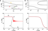Fig. 2 Coplanar equilibrium solutions and examples of orbital evolution using the full-space (nonlinear) disk gravity model (a) and the approximate linear model (b). The upper panels of (a) and (b) show equilibrium solutions as a function of ϵ⋆d (or ${ϵ}_{\star \mathrm{d}}^{\mathrm{\prime }}$) for ψ⋆0 = 70°. In (a), the coplanar equilibria (P2, P3, P4, and P5) and bifurcations (B1 and B2) are denoted. The lower panels of (a) and (b) show the evolution of the stellar obliquity through numerical integrations of corresponding secular equations. The dashed curves in the two panels represent the evolution of the equilibria.

3.2 Stability of equilibria

Near the equilibrium (${\overline{\mathit{l}}}_1,{\overline{\mathit{e}}}_1=\mathbf{0}$), the angular momentum l₁ can be written as ${\mathit{l}}_1={\overline{\mathit{l}}}_1+\mathrm{\Delta }{\mathit{l}}_1$, where Δl₁ denotes a small disturbance from the equilibrium. The secular equations to the first order in Δl₁ and e₁ (e₁ = 0 + Δe₁) are written as $$\begin{array}{rl}\mathrm{\Delta }{\dot{\mathit{l}}}_1=& -({\overline{\mathit{l}}}_1\cdot {\hat{\mathit{s}}}_{\star }){\hat{\mathit{s}}}_{\star }\times \mathrm{\Delta }{\mathit{l}}_1-(\mathrm{\Delta }{\mathit{l}}_1\cdot {\hat{\mathit{s}}}_{\star }){\hat{\mathit{s}}}_{\star }\times {\overline{\mathit{l}}}_1\\ & -\frac{1}{{ϵ}_{\star \mathrm{d}}}\frac{1}{S_1^3}{({\overline{\mathit{l}}}_1\cdot {\hat{\mathit{l}}}_{\mathrm{d}})}^2(\mathrm{\Delta }{\mathit{l}}_1\cdot {\hat{\mathit{l}}}_{\mathrm{d}}){\hat{\mathit{l}}}_{\mathrm{d}}\times {\overline{\mathit{l}}}_1-\frac{1}{{ϵ}_{\star \mathrm{d}}}\frac{1}{S_1}\\ & \times (1-\frac{\pi }{4}{S}_1)[({\overline{\mathit{l}}}_1\cdot {\hat{\mathit{l}}}_{\mathrm{d}}){\hat{\mathit{l}}}_{\mathrm{d}}\times \mathrm{\Delta }{\mathit{l}}_1+(\mathrm{\Delta }{\mathit{l}}_1\cdot {\hat{\mathit{l}}}_{\mathrm{d}}){\hat{\mathit{l}}}_{\mathrm{d}}\times {\overline{\mathit{l}}}_1],\\ {\dot{\mathit{e}}}_1=& -\frac{1}{2}[1-5{({\overline{\mathit{l}}}_1\cdot {\hat{\mathit{s}}}_{\star })}^2]{\overline{\mathit{l}}}_1\times {\mathit{e}}_1-({\overline{\mathit{l}}}_1\cdot {\hat{\mathit{s}}}_{\star }){\hat{\mathit{s}}}_{\star }\times {\mathit{e}}_1\\ & +\frac{1}{{ϵ}_{\star \mathrm{d}}}\frac{1}{S_1}\{[1-\frac{\pi }{16}{S}_1(8-S_1^2)]{\overline{\mathit{l}}}_1\times {\mathit{e}}_1-(1-\frac{\pi }{4}S)\\ & \times ({\hat{\mathit{l}}}_{\mathrm{d}}\cdot {\overline{\mathit{l}}}_1){\hat{\mathit{l}}}_{\mathrm{d}}\times {\mathit{e}}_1+(1-\frac{3\pi }{8}{S}_1)({\hat{\mathit{l}}}_{\mathrm{d}}\cdot {\mathit{e}}_1){\hat{\mathit{l}}}_{\mathrm{d}}\times {\overline{\mathit{l}}}_1\}.\end{array}$$(27)

Note that the linearized evolution of Δl₁ and e₁ are decoupled, as shown in Eq. (27). This decoupling allows us to focus solely on the stability of the equilibrium in l₁ and defer the analysis of e₁ to future work.

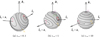Fig. 3 Phase portraits for ψ⋆0 = 70° and ϵ⋆d = 0.1 (a), 1.0 (b), and 10.0 (c) displayed on the unite sphere. These portraits were generated by plotting level curves of the perturbing Hamiltonian from Eq. (20) with |l1| = 1. The orientations of ${\hat{\mathit{s}}}_{\star }$ and ${\hat{\mathit{l}}}_{\mathrm{d}}$ are shown, along with the norm of the principal plane. Equilibria are marked by colored points, which correspond to the equilibrium solutions identified in Fig. 2a.

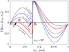Fig. 4 Values of f(ψ1⋆; ψ⋆0, ϵ⋆d) defined by Eq. (23) as functions of ψ1⋆ and ϵ⋆d for ψ⋆0 = 70°. The red and blue curves represent the critical ϵ⋆d that trigger the bifurcations B1 and B2, respectively, which are characterized by f = 0 and df/dψ1⋆ = 0. The two bifurcations are further distinguished by the sign of ${\mathrm{d}}^{2}f/\mathrm{d}{\psi }_{1\star }^2$: B1 (<0) and B2 (>0).

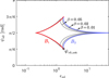Fig. 5 Bifurcation curves in the (ϵ⋆d, ψ⋆0) space obtained using the bifurcation conditions (Eq. (26)). Curves are shown for three disk softening scales: β = 0.01, 0.02, and 0.05. For β = 0.01, the bifurcation curves of B1 and B2 are in red and blue, respectively. Critical values of ψ⋆0 are also marked.

3.2.1 Stability of the orthogonal equilibrium

For the orthogonal equilibrium, where ${\hat{\mathit{s}}}_{\star }\cdot {\overline{\mathit{l}}}_1={\hat{\mathit{l}}}_{\mathrm{d}}\cdot {\overline{\mathit{l}}}_1=0$ and S₁ ≈ 1, the first part of Eq. (27) becomes $$\mathrm{\Delta }{\dot{\mathit{l}}}_1=-(\mathrm{\Delta }{\mathit{l}}_1\cdot {\hat{\mathit{s}}}_{\star }){\hat{\mathit{s}}}_{\star }\times {\overline{\mathit{l}}}_1-\frac{1}{{ϵ}_{\star \mathrm{d}}}(1-\frac{\pi }{4})(\mathrm{\Delta }{\mathit{l}}_1\cdot {\hat{\mathit{l}}}_{\mathrm{d}}){\hat{\mathit{l}}}_{\mathrm{d}}\times {\overline{\mathit{l}}}_1.$$(28)

The constant $l_1^2+e_1^2=1$ results in ${\overline{\mathit{l}}}_1\cdot \mathrm{\Delta }{\mathit{l}}_1=0$ at the linear level. Consequently, the linearized dynamics are confined to a two-dimensional subspace.

By projecting Δl₁ onto ${\hat{\mathit{s}}}_{\star }$ and ${\hat{\mathit{l}}}_{\mathrm{d}}$, and defining $x_1=\mathrm{\Delta }{\mathit{l}}_1\cdot {\hat{\mathit{s}}}_{\star }$ and $x_2=\mathrm{\Delta }{\mathit{l}}_1\cdot {\hat{\mathit{l}}}_{\mathrm{d}}$, we formulate the system in terms of the state vector x = [x₁ x₂]^T. The dynamics of x is governed by $\dot{\mathit{x}}=A\mathit{x}$, where A is given by $$A=\left[\begin{array}{cc}0& -\frac{1}{{ϵ}_{\star \mathrm{d}}}(1-\frac{\pi }{4}){\hat{\mathit{s}}}_{\star }({\hat{\mathit{l}}}_{\mathrm{d}}\times {\overline{\mathit{l}}}_1)\\ -{\hat{\mathit{l}}}_{\mathrm{d}}({\hat{\mathit{s}}}_{\star }\times {\overline{\mathit{l}}}_1)& 0\end{array}\right].$$(29)

The eigenvalues are $${\lambda }^2=-\frac{1}{{ϵ}_{\star \mathrm{d}}}(1-\frac{\pi }{4}){\left[({\hat{\mathit{s}}}_{\star }\times {\hat{\mathit{l}}}_{\mathrm{d}}){\overline{\mathit{l}}}_1\right]}^2.$$(30)

It is obvious that λ² < 0, and therefore the orthogonal equilibrium P₁ is linearly stable to variations in l₁.

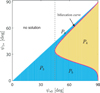Fig. 6 Stability of the circular coplanar equilibria as functions of ψ⋆0 and ψ1⋆ for ψ1⋆ ∈ (0, π/2), calculated using the stability condition, Eq. (32). Blue points represent stable equilibria where λ2 < 0, and yellow points indicate unstable equilibria where λ2 > 0. The red curve presents the bifurcation curve in the (ψ⋆0, ψ1⋆) space, derived from the bifurcation conditions (Eq. (26)).

3.2.2 Stability of the coplanar equilibria

At the coplanar circular equilibrium, we performed the projections $x_1=({\hat{\mathit{l}}}_{\mathrm{d}}\times {\hat{\mathit{s}}}_{\star })\cdot \mathrm{\Delta }{\mathit{l}}_1$ and $x_2=[({\hat{\mathit{l}}}_{\mathrm{d}}\times {\hat{\mathit{s}}}_{\star })\times {\overline{\mathit{l}}}_1]\cdot \mathrm{\Delta }{\mathit{l}}_1$ to the first part of (27). The eigenvalues are given by $$\begin{array}{rl}{\lambda }^2=& [{\cos }^2{\psi }_{1\star }+\frac{1}{{ϵ}_{\star \mathrm{d}}}\frac{1}{S_1}(1-\frac{\pi }{4}{S}_1){\cos }^2({\psi }_{\star 0}-{\psi }_{1\star })]\\ & \times [-\cos 2{\psi }_{1\star }-\frac{1}{{ϵ}_{\star \mathrm{d}}}\frac{1}{S_1}(1-\frac{\pi }{4}{S}_1)\cos 2({\psi }_{\star 0}-{\psi }_{1\star })\\ & +\frac{1}{4}\frac{1}{{ϵ}_{\star \mathrm{d}}}\frac{1}{(S_1-h)S_1^2}{\sin }^{2}2({\psi }_{\star 0}-{\psi }_{1\star })].\end{array}$$(31)

Utilizing the equilibrium conditions, Eq. (23), we reformed the eigenvalues as functions of ψ_⋆0 and ψ_1⋆, given by $$\begin{array}{rl}{\lambda }^2=& [{\cos }^2{\psi }_{1\star }+\frac{1}{2}\sin 2{\psi }_{1\star }\cot ({\psi }_{\star 0}-{\psi }_{1\star })]\\ & \times [-\sin 2{\psi }_{\star 0}/\sin 2({\psi }_{\star 0}-{\psi }_{1\star })\\ & +\frac{1}{S_1(S_1-\beta )(4-\pi S_1)}\sin 2{\psi }_{1\star }\sin 2({\psi }_{\star 0}-{\psi }_{1\star })].\end{array}$$(32)

If ψ_1⋆ is in the range (π/2, π/2 + ψ_⋆0), we find that λ² > 0, implying the equilibrium P₂ is unstable, being a saddle point. The stability of the equilibria for ψ_1⋆ in the range (0, ψ_⋆0) is illustrated in Fig. 6 by utilizing Eq. (32). It is shown that P₃ and P₅ are stable, and P₄ is unstable, also being a saddle point. These findings are consistent with the phase portraits presented in Fig. 3.

4 Application to hierarchical systems

In the preceding sections, we have considered a simple system involving only one planet. In this section, we extend our analysis to hierarchical systems, characterized by the presence of a distant outer massive perturbing companion.

4.1 Equilibria and bifurcations

In the hierarchical three-body system with L₁ ≪ L₂, the outer planet is primarily coupled to the disk, leading to ${\hat{\mathit{l}}}_2\approx {\hat{\mathit{l}}}_{\mathrm{d}}$. This approximation allows us to only focus on the evolution of the inner orbit. The perturbing Hamiltonian (assuming e₁ = 0) under this consideration is expressed as: $${\mathrm{\Phi }}_{\mathrm{c}\mathrm{i}\mathrm{r}\mathrm{c}}=-\frac{{\varphi }_{\star }}{2}{({\mathit{l}}_1\cdot {\hat{\mathit{s}}}_{\star })}^2+{\varphi }_{\mathrm{d}}{S}_1(1-\frac{\pi }{8}{S}_1)-\frac{{\varphi }_{12}}{2}{({\mathit{l}}_1\cdot {\hat{\mathit{l}}}_2)}^2.$$(33)

Then, the circular equilibria can be obtained from the equation $$({\mathit{l}}_1\cdot {\hat{\mathit{s}}}_{\star }){\hat{\mathit{s}}}_{\star }\times {\mathit{l}}_1+[\frac{1}{{ϵ}_{\star \mathrm{d}}}\frac{1}{S_1}(1-\frac{\pi }{4}{S}_1)+\frac{1}{{ϵ}_{\star \mathrm{p}}}]({\hat{\mathit{l}}}_{\mathrm{d}}\cdot {\hat{\mathit{l}}}_1){\hat{\mathit{l}}}_{\mathrm{d}}\times {\mathit{l}}_1=0.$$(34)

Here ϵ_⋆d is defined by Eq. (22), and ϵ_⋆p is defined as the relative magnitude between the stellar oblateness and the perturbation from the outer companion: $${ϵ}_{\star \mathrm{p}}=\frac{{\varphi }_{1\star }}{{\varphi }_{12}}=2\frac{m_{\star }}{m_2}\frac{J_2{R}_{\star }^2}{a_1^2}\frac{a_2^3{(1-e_2^2)}^{3/2}}{a_1^3}.$$(35)

From Eq. (34), it is evident that the introduction of the outer perturber does not alter the types of equilibrium solutions – coplanar or orthogonal equilibria. However, it does modify the structure of the phase space depending on the value ϵ_⋆p, as illustrated in Fig. 7. For the high primordial obliquity ψ_⋆0 = 70°, the phase space structure at ϵ_⋆d ~ 1 differs between the case with ϵ_⋆p = 10.0 (upper panels) and the case with ϵ_⋆p = 1.0 (lower panels). This arises because bifurcations occur in the former case but not in the latter. As shown, when ϵ_⋆p = 1.0, bifurcations are inhibited and, as a result, the topology of the phase space does not change with ϵ_⋆d. We therefore investigated how the parameter ϵ_⋆p influences the dynamical bifurcation-induced effect and stability of the equilibria.

Constraining to coplanar equilibria, the equilibrium equation (34) becomes $$\begin{array}{r}g({\psi }_{1\star };{\psi }_{\star 0},{ϵ}_{\star \mathrm{d}},{ϵ}_{\star \mathrm{p}})=\sin 2{\psi }_{1\star }-[\frac{1}{{ϵ}_{\star \mathrm{d}}}\frac{1}{S_1}(1-\frac{\pi }{4}{S}_1)\\ +\frac{1}{{ϵ}_{\star \mathrm{p}}}]\sin 2({\psi }_{\star 0}-{\psi }_{1\star })=0\end{array}.$$(36)

The bifurcation condition is then $$\{\begin{array}{l}g({\psi }_{1\star };{\psi }_{\star 0},{ϵ}_{\star \mathrm{d}},{ϵ}_{\star \mathrm{p}})=0,\\ \mathrm{d}g({\psi }_{1\star };{\psi }_{\star 0},{ϵ}_{\star \mathrm{d}},{ϵ}_{\star \mathrm{p}})/\mathrm{d}{\psi }_{1\star }=0.\end{array}$$(37)

Note this condition depends on three parameters: ψ_⋆0, ϵ_⋆d, and ϵ_⋆p.

By using this condition, the bifurcation curves in the (ϵ_⋆d, ϵ_⋆p) and (ψ_⋆0, ϵ_⋆p) spaces are depicted in Fig. 8. In the absence of an outer perturbation, i.e., ϵ_⋆p = ∞, the bifurcations depend solely on the primordial misalignment angle ψ_⋆0, since ϵ_⋆d typically sweeps from an extremely small value to a much larger value as the disk disperses, as discussed above. When an outer perturbation is considered, both ψ_⋆0 and ϵ_⋆p play critical roles in determining the occurrence of bifurcations. Bifurcations only occur if ϵ_⋆p surpasses a specific threshold that depends on ψ_⋆0, as shown in Fig. 8a. Moreover, as ψ_⋆0 decreases, the bifurcation region associated with ϵ_⋆d narrows and eventually disappears.

Figure 8b shows the critical misalignment angle, ${\psi }_{\star 0,\text{crit}}^P$, as a function of ϵ_⋆p. As ${ϵ}_{\star \mathrm{p}}\to \mathrm{\infty },{\psi }_{\star 0,\text{\hspace{0.17em}crit\hspace{0.17em}}}^P\to {\psi }_{\star 0,\text{\hspace{0.17em}crit\hspace{0.17em}}}\approx {44.6}^{\circ }$ for β = 0.01. Conversely, ${\psi }_{\star 0,\text{crit}}^P$ increases inversely with ϵ_⋆p. For example, when ϵ_⋆p is about 5.0 and 2.0, ψ_⋆0,crit becomes 50° and 60°, respectively. Finally, when ${ϵ}_{\star \mathrm{p}}\to 1.0,{\psi }_{\star 0,\text{\hspace{0.17em}crit\hspace{0.17em}}}^P\to {90}^{\circ }$. This condition can be confirmed by substituting ψ_⋆0 = 90° into Eqs. (37), resulting in $$(1-\frac{1}{{ϵ}_{\star \mathrm{p}}})\frac{4}{(4-\pi S_1)S_1}\sin {\psi }_{1\star }\sin 2{\psi }_{1\star }=0.$$(38)

Since ψ_1⋆ < ψ_⋆0 = 90°, the above equation gives ϵ_⋆p = 1. As a result, if ϵ_⋆p < 1, the bifurcations are completely inhibited for any value of ψ_⋆0.

Observations indicate that about 40% of close-in small planets have outer giant planet companions (Rosenthal et al. 2022). In Table 1, we present the parameters ϵ_⋆p and the corresponding values of ${\psi }_{\star 0,\text{crit}}^P$ for several hierarchical systems that include an outer giant planet, assuming typical pre-main-sequence stellar parameters (Bouvier et al. 2014). The stellar oblateness J₂ can be estimated by $$J_2=\frac{2k_{\mathrm{q}\star }{\mathrm{\Omega }}_{\star }^2}{3G{m}_{\star }/R_{\star }^3},$$(39)

where k_q⋆ is the stellar apsidal motion constant (k_q⋆ ≃ 0.1 for fully convective stars), and Ω_⋆ is the stellar rotational angular velocity.

From Cases I–IV, it is evident that a giant planet located in the outer region (1–10 au) generally results in ϵ_⋆p > 1 for the inner, close-in planet. That is, the outer companions typically modify the critical ψ_⋆0 for bifurcations, but are generally unable to completely prevent them.

The evolution of inclinations between the inner and outer orbits for Cases I and III is depicted in Fig. 9a. In Case I, ψ_⋆0 is set as 65°, larger than the critical obliquity estimated to be ${\psi }_{\star 0,\text{crit}}^P$ = 45.3°. This results in large-amplitude mutual inclinations as a result of encountering the bifurcation B₂, which is reflected by the jump in the evolutionary path of the equilibrium in the figure. In Case III, ${\psi }_{\star 0\text{,crit}}^P$ is approximately 71.8°. Here, the scenarios of ψ_⋆0 = 65° and 78° are expected to fall within the adiabatic and separatrix-crossing regimes, respectively, leading to distinct evolutionary behaviors as shown in the figure. Note in the adiabatic regime, if ψ_⋆0 is close to ${\psi }_{\star 0,\text{crit}}^P$ – as is the case of ψ_⋆0 = 65° – small nonadiabatic components can still develop, due to the comparable timescales of the equilibrium transition (which becomes small at certain epoch of ϵ_⋆d ~ 1 if ${\psi }_{\star 0}\to {\psi }_{\star 0,\text{crit}}^P$) and the orbit precession.

The estimations of ϵ_⋆p and ${\psi }_{\star 0,\text{crit}}^P$ have also been conducted for the K2-290A and HD 3167 systems, both of which are characterized by multiple coplanar planets with high stellar obliquities. Recent studies suggest that primordial disk misalignments could be the causes of the two unusual system architectures (Hjorth et al. 2021; Fu & Wang 2024). Given that our study focuses on the dynamical evolution subsequent to the formation of primordial misalignments, our analysis can provide additional examinations on these proposed dynamical processes.

The K2-290A system, comprising two coplanar planets in a retrograde configuration, exhibits a stellar obliquity of ψ_⋆ = 124° ± 6°. Two scenarios for the host star’s parameters, referred to as K2-290A(1) and K2-290A(2), are considered and detailed in Table 1. In K2-290A(1), a strong stellar oblateness is assumed with R_⋆ = 2.5 R_⊙ and P_⋆ = 3 days, resulting in ${\psi }_{\star 0,\text{crit}}^P$ ≈ 56.8°. Therefore, bifurcations are avoided if ψ_⋆0 < 56.8° or > 123.2°. The inclination evolution for ψ_⋆0 = 110° and 124° are illustrated in Fig. 9b. In the case of ψ_⋆0 = 124°, considering the decay of stellar oblateness, a coplanar configuration with high stellar obliquity, ψ_⋆ ≈ 124°, can be achieved. Conversely, the case of ψ_⋆0 = 110° fails to produce coplanar configuration.

In K2-290B(2), a weaker stellar oblateness is assumed, resulting in ϵ_⋆p < 1, which prevents bifurcations for any value of ψ_⋆0. This ensures coplanarity more readily. Consequently, we conclude that for a significant portion of the parameter space of R_⋆ and P_⋆, the evolution remains adiabatic at such high primordial obliquities (ψ_⋆0 ~ 124°), supporting the hypothesis that primordial misalignment is a plausible origin for the observed configuration.

In the HD 3167 system, the inner and outer orbits are nearly perpendicular with a mutual inclination $i_{\text{mut\hspace{0.17em}}}\approx {102.3}_{+{7.4}^{\circ }}^{-{8.0}^{\circ }}$. Therefore, unlike the K2-290A system, which requires an adiabatic process to ensure coplanarity, the HD-3167 system demands a separatrix-crossing process to achieve such a high mutual inclination. As indicated in Table 1, even assuming a relatively weak initial stellar oblateness, we have ϵ_⋆p ≫ 1. This suggests that large-amplitude mutual inclinations between the inner and outer orbits can be robustly established at high ψ_⋆0 through the bifurcation-induced effect (Fu & Wang 2024).

In Table 1, we also provide the parameter ϵ_⋆p when the outer perturbation is solely contributed by the outer disk, under nonhomologous disk dissipation conditions. It shows that the perturbation exerted by the outer disk is relatively weak, exerting only a minor influence on the critical primordial obliquity for the bifurcations.

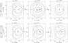Fig. 7 Phase portraits for ψ⋆0 = 70° presented in the (ψ1⋆ cos Δh, ψ1⋆ sin Δh) plane, where Δh represents the difference in the longitudes of the ascending node between the inner and outer orbits. These portraits were generated by plotting level curves of the perturbing Hamiltonian (Eq. (33)). In the upper panels, ϵ⋆p = 10.0 and ϵ⋆d = 0.1, 1.5, and 5.0, respectively. In the lower panels, ϵ⋆p = 1.0 with the same variations in ϵ⋆d. Equilibrium points are indicated with colored markers. The projections of ${\hat{\mathit{s}}}_{\star }$ and ${\hat{\mathit{l}}}_{\mathrm{d}}$ on this plane are denoted by filled triangles.

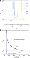Fig. 8 Bifurcation curves for hierarchical systems. (a) Bifurcation curves for several high values of ψ⋆0 presented in the (ϵ⋆d, ϵ⋆p) space. The dashed and solid curves represent the bifurcations B1 and B2, respectively. (b) Bifurcation curves in the (ψ⋆0, ϵ⋆p) space, where the curves for B1 and B2 degenerate into one curve. The softening scale is chosen as β = 0.01.

4.2 Stability

4.2.1 The orthogonal equilibrium

Building on the methodologies outlined in Section 3, we can easily determine that the orthogonal equilibrium P₁ is linearly stable in response to variations in l₁.

4.2.2 The coplanar equilibria

For the coplanar equilibria, the stability to variations in l₁ can be determined by the eigenvalues given by $$\begin{array}{rl}{\lambda }^2& =[{\cos }^2{\psi }_{1\star }+\frac{1}{2}\sin 2{\psi }_{1\star }\cot ({\psi }_{\star 0}-{\psi }_{1\star })]\\ & \times [\frac{-\sin {\psi }_{\star 0}}{\sin 2({\psi }_{\star 0}-{\psi }_{1\star })}+\frac{1}{S_1(S_1-\beta )(4-\pi S_1)}\\ & \times (\sin 2{\psi }_{1\star }-\frac{1}{{ϵ}_{\star \mathrm{p}}}\sin 2({\psi }_{\star 0}-{\psi }_{1\star }))\sin 2({\psi }_{\star 0}-{\psi }_{1\star })].\end{array}$$(40)

If ψ_1⋆ lies within the interval (π/2, π), the expression within the first square bracket on the right-hand side of Eq. (40) is positive. Applying Eq. (36), we find that sin 2ψ_1⋆ – sin 2(ψ_⋆0 − ψ_1⋆)/ϵ_⋆p > 0, ensuring the term in the second square bracket is also positive. Consequently, the equilibrium, P₂, is unstable with respect to changes in l₁.

The stability of the equilibria for ψ_1⋆ in the range (0, π/2) is illustrated in Fig. 10 by using Eq. (40). This stability analysis aligns with the behaviors observed in the phase portraits and indicated by the bifurcation curves. Specifically, if ϵ_⋆p > 1.0, the equilibria P₃ and P₅ are stable, whereas P₄ is unstable. When ϵ_⋆p < 1.0, bifurcations are inhibited, resulting in P₃ being the sole stable equilibrium.

5 Application to compact multi-planet systems

Over the past decade, a large amount of super-Earth and sub-Neptune planets—bodies with size ranging from 1 to 4R_⊕—has been discovered by Kepler mission. These planets are predominantly found in multi-planet systems that typically exhibit compact orbital configurations. In this section, we extend our analysis to these compact multi-planet systems.

5.1 Equilibria of multiple planets

The secular Hamiltonian that governs the secular evolution of n_p planets in a compact configuration is given by $$\mathrm{\Phi }=\sum _{i=1}^{n_{\mathrm{p}}}{\mathrm{\Phi }}_{\star ,i}+{\mathrm{\Phi }}_{\mathrm{d},i}+\sum _{i\ne j}{\mathrm{\Phi }}_{ij},$$(41)

where Φ_ij is the interaction potential between planets i and j through Laplace-Lagrange theory (Eq. (8)). Then, by using Eqs. (6) and (7), the secular equations of motion can be obtained.

The equilibrium conditions should be established for n_p planets, each with planetary mass m_i, semimajor axis a_i (where i = 1, 2 . . ., n_p and a₁ < . . . a_np), and a circular orbit (e_i = 0). The equilibrium for the i-th planet satisfies $$\begin{array}{rl}& ({\mathit{l}}_i\cdot {\hat{\mathit{s}}}_{\star }){\hat{\mathit{s}}}_{\star }\times {\mathit{l}}_i+\frac{1}{{ϵ}_{\star \mathrm{d},i}}\frac{1}{S_i}(1-\frac{\pi }{4}{S}_i)({\hat{\mathit{l}}}_{\mathrm{d}}\cdot {\hat{\mathit{l}}}_i){\hat{\mathit{l}}}_{\mathrm{d}}\times {\mathit{l}}_i\\ & +\sum _{j\ne i}\frac{1}{{ϵ}_{\star j,i}}({\hat{\mathit{l}}}_j\cdot {\hat{\mathit{l}}}_i){\hat{\mathit{l}}}_j\times {\mathit{l}}_i=0,\end{array}$$(42)

where ϵ_⋆j,i is defined by $${ϵ}_{\star j,i}=\frac{{\varphi }_{\star i}}{{\varphi }_{ij}}=\{\begin{array}{l}6\frac{m_{\star }}{m_j}{\left(\frac{a_j}{a_i}\right)}^2\frac{J_2{R}_{\star }^2}{a_i^2}\frac{1}{b_{3/2}^{(1)}\left(a_i/a_j\right)},a_i<a_j,\\ 6\frac{m_{\star }}{m_j}\frac{J_2{R}_{\star }^2}{a_i{a}_j}\frac{1}{b_{3/2}^{(1)}\left(a_j/a_i\right)},a_i>a_j.\end{array}$$(43)

Focusing solely on the coplanar equilibrium solutions, Eq. (42) simplifies to $$\begin{array}{rl}{g}_i\triangleq & \sin 2{\psi }_{i\star }-\frac{1}{{ϵ}_{\star \mathrm{d},i}}\frac{1}{S_i}(1-\frac{\pi }{4}{S}_i)\sin 2({\psi }_{\star 0}-{\psi }_{i\star })\\ & -\sum _{j\ne i}\frac{1}{{ϵ}_{\star j,i}}\sin 2({\psi }_{j\star }-{\psi }_{i\star })=0.\end{array}$$(44)

Determining the equilibrium solutions for n_p planets involves solving n_p coupled nonlinear equations – a computationally challenging task. This study instead prioritizes identifying whether planetary orbits undergo bifurcation-induced evolution, a critical factor governing system evolution pathways. We therefore focused on establishing bifurcation conditions in compact multi-planet systems.

Given the complexity of a thorough exploration of the parameter space, we restricted our analysis to qualitative assessments to establish a approximate criterion for the system’s evolution pattern. Typically, the innermost orbit, which is most influenced by stellar oblateness, is the first to experience the bifurcation at high primordial obliquities. Consequently, motivated by the hierarchical systems, we utilized the parameter ϵ_⋆p,1 ≜ ∑_j ϵ_⋆j,1 (where ϵ_⋆j,1 is defined similar to Eq. (35)) and ψ_⋆0 to characterize the system’s evolution.

5.2 Numerical simulations

To establish a preliminary criterion, we conducted numerical simulations on several representative compact multi-planet systems with varying order of ϵ_⋆p. The system parameters are detailed in Table 2.

In Case I, where ϵ_⋆p,1 ≈ 8.12, the effective ${\psi }_{\star 0\text{,crit}}^P$ for the innermost planet is estimated to be 48.1°. As depicted in Fig. 11a, when ψ_⋆0 = 45°, all planets undergo adiabatic evolution, following their equilibrium paths. Conversely, at ψ_⋆0 = 60°, the system has experienced the separatrix-crossing behavior, leading to significant stellar obliquities and mutual planetary inclinations. A similar behavior is observed in Case II, as shown in Fig. 11b, where ϵ_⋆p,1 ≈ 1.56 and ${\psi }_{\star 0,\text{crit}}^P$ is estimated to be about 64.5°. Therefore, we conclude that if ϵ_⋆p,1 > 1, the critical angle ${\psi }_{\star 0,\text{crit}}^P$ serves as a reliable indicator of the system’s evolutionary pattern, analogous to the hierarchical systems discussed in Sect. 4.

For ϵ_⋆p,1 ≲ 1, the bifurcations in hierarchical systems are almost entirely inhibited. However, in compact multi-planet systems, the coupled evolution among the planetary orbits allows the separatrix-crossing behaviors to persist at sufficiently high ψ_⋆0, resulting in moderate stellar oblateness and mutual inclinations, as illustrated in Fig. 11c for Cases III.

When ϵ_⋆p,1 ≪ 1, interplanetary coupling dominates over perturbations from stellar oblateness, causing the planets to evolve collectively as a single plane. Consequently, the system’s evolution resembles that of a single-planet system, as discussed in 3. The resulting orbital architectures feature coplanar planets with either low stellar obliquities (${\psi }_{\star 0}<{\psi }_{\star 0,\text{crit}}^{\ast }$; Fig. 11d), upper panels) or high stellar obliquities (${\psi }_{\star 0}>{\psi }_{\star 0,\text{\hspace{0.17em}crit\hspace{0.17em}}}^{\ast }$; Fig. 11d, lower panels). Note that ${\psi }_{\star 0,\text{crit}}^{\ast }$ can differ from the critical obliquity ψ_⋆0,crit (≈ 44.6°) derived for single-planet systems due to the planetary interactions.

We highlight that in the regime of ϵ_⋆p,1 ≪ 1, planets remain coplanar despite undergoing separatrix-crossing evolution at high ψ_⋆0, thereby preserving orbital stability (no eccentricity excitations). Consequently, stable, coplanar multi-planet systems exhibiting high stellar obliquities can emerge in this regime.

In the separatrix-crossing regime, large mutual inclinations between planetary orbits may compromise the accuracy of the Laplace-Lagrange approximation. Nonetheless, this framework remains useful for identifying bifurcations and distinguishing between adiabatic and separatrix-crossing evolution. On the other hand, while our simulations neglect eccentricity vector evolution, we emphasize that in this regime, planetary orbits could experience eccentricity excitations due to large-amplitude librating mutual inclinations established during disk dispersal. These excitations can trigger orbital destabilization. For comprehensive modeling of secular planet-planet interactions, the Gauss ring averaging method provides an efficient approach to simulating long-term evolution (Touma et al. 2009), though its implementation falls beyond the scope of this study.

To evaluate the prevalence of different regimes (ϵ_⋆p,1 > 1, ϵ_⋆p,1 ≲ 1, or ϵ_⋆p,1 ≪ 1) in compact multi-planet systems, we computed ϵ_⋆p,1 as a function of the innermost semimajor axis a₁ using typical system parameters, as shown in Fig. 12. Our analysis considered two pre-main-sequence stellar oblateness values: a stronger case J₂ = 7.97 × 10⁻⁴ and a weaker case J₂ = 1.46 × 10⁻⁴, assuming regular orbital spacings. According to this figure, systems with a₁ ≲ 0.1 au predominantly fall within the regime of ϵ_⋆p,1 > 1; systems with 0.1 ≲ a₁ ≲ 0.2–0.25 au mostly result in ϵ_⋆p,1 ≲ 1; and systems with a₁ ≳ 0.2–0.25 au generally lead to ϵ_⋆p,1 ≪ 1.

Combining these estimates with Kepler multi-planet system statistics from the NASA Exoplanet Archive, as shown in Fig. 12, we find that > 90% compact systems have a₁ < 0.15. This indicates that that during early evolution, most systems reside in either the ϵ_⋆p,1 > 1 or ϵ_⋆p,1 ≲ 1 regime. In contrast, systems featured by ϵ_⋆p,1 ≪ 1 are rare. Consequently, while primordial misalignments may be common, coplanar multi-planet systems exhibiting high stellar obliquities (requiring ϵ_⋆p,1 ≪ 1) remain uncommon-– consistent with observational evidence that Kepler multi-planet systems generally exhibit low stellar obliquities.

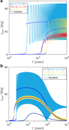Fig. 9 Evolution of orbital inclinations between inner and outer orbits for hierarchical three-body systems obtained by integrating the secular equations for circular orbits. The system parameters are detailed in Table 1. We set the timescale of the disk dissipation (τd) to 1 × 104 yr. In (a), the decay of host stellar oblateness is not considered. In (b), the oblateness of the host star decays due to its radius contraction: R⋆ = R⋆ (0)/(1 + t/τR⋆)−1/3, where τR⋆ = 1 Myr. The temporal evolution of the equilibrium that dominates the planet’s evolution is depicted for each system. Notably, a jump in the equilibrium trajectory signifies an encounter with bifurcation B2.

6 Discussion and conclusion

We have studied the secular dynamics of planetary systems in the presence of misaligned protoplanetary disks. More specifically, we have presented an analytical study of the basic mechanism – the bifurcation-induced effect due to the saddle-node bifurcation occurring during the disk dispersal – that robustly leads to separatrix-crossing behavior, thus causing large-amplitude librating mutual planetary inclinations.

The separatrix-crossing behavior induced by this dynamical bifurcation is theoretically independent of the timescale of disk dispersal but depends on the primordial stellar obliquities. This is in contrast with the mechanism proposed by Spalding & Millholland (2020), who considered a similar dynamical problem involving planet-disk interactions. In their study, the transition between adiabatic and nonadiabatic regimes is explicitly dependent on the relative timescales of disk dispersal and orbital precession. The underlying principle is intuitive: if τ_d > τ_⋆1 (where τ_⋆1 represents the minimum orbital precession timescale induced by stellar oblateness), planets adiabatically track their equilibrium paths. Conversely, if τ_d ≲ τ_⋆1, planets undergo nonadiabatic evolution because the equilibria evolve too rapidly for the planets to follow them effectively. It is evident that this process is independent of the specific values of the primordial misalignment angles.

The qualitative differences observed between these two studies stem from the distinct secular gravitational models of the protoplanetary disks employed. Spalding & Millholland (2020) adopted the linear disk model (Eq. (12)), which ignores a critical nonlinear factor and is only valid when planets remain close to the disk plane (Hahn 2003; Zanazzi & Lai 2018). In contrast, our work adopts a more comprehensive secular model that is feasible for the full physical space (Schulz 2012; Fu & Wang 2024). As a result, Spalding & Millholland (2020) failed to identify the dynamical bifurcations studied here.

Synthesizing the findings from the two studies, we conclude that both the timescale of disk dispersal and the presence of dynamical bifurcations are critical in determining the evolutionary patterns of planetary systems. Specifically, if τ_d ≲ τ_⋆1, the evolution is expected to be nonadiabatic independent of other parameters, producing significant mutual planetary inclinations. Conversely, if τ_d > τ_⋆1, the nature of the evolution depends on the initial conditions: when ψ_⋆0 < ψ_⋆0,crit, planets adiabatically follow their equilibria, maintaining coplanarity; when ψ_⋆0 > ψ_⋆0,crit, the bifurcation leads to separatrix-crossing behaviors, forming large-amplitude librating inclinations. Current observations suggest that the timescale for photoevaporation-driven dispersal of the inner regions of the disk ranges approximately from 10² to 10⁵ yr. During the early epoch, the minimum orbit precession timescale (τ_⋆1), driven by young stellar oblateness, is typically 10² to 10³ yr for a₁ < 0.1 au. Therefore, only at the lower limit of these potential τ_d is the nonadiabatic process induced by the mechanism proposed by Spalding & Millholland (2020). In other cases, the evolution patterns are determined by the framework proposed in this study.

In a simple system with a single planet, the critical primordial misalignment angle, ψ_⋆0,crit, for triggering the bifurcation is about 44.6° for a disk softening scale of β = 0.01. This critical angle is slightly influenced by the value of β. A larger β leads to a larger ψ_⋆0,crit.

Applying this to two-planet systems with hierarchical configurations, the introduction of an outer perturbation modifies this fundamental mechanism. We introduced a new parameter, ϵ_⋆p, to quantify the relative magnitude of stellar oblateness versus the external perturbation, thus characterizing the modified parameter space. Our analysis reveals that when ϵ_⋆p > 1, the critical ψ_⋆0 for the bifurcation increases from ψ_⋆0,crit to a higher value, denoted as ${\psi }_{\star 0,\text{crit}}^{\mathrm{p}}$. This value increases as ϵ_⋆p decreases. As ${ϵ}_{\star \mathrm{p}}\to 1,{\psi }_{\star 0,\text{\hspace{0.17em}crit\hspace{0.17em}}}^{\mathrm{p}}\to {90}^{\circ }$. If ϵ_⋆p < 1, the bifurcation is entirely inhibited for any value of ψ_⋆0.

This mechanism also operates in compact multi-planet systems. We propose a rough criterion to characterize the system evolution: if ϵ_⋆p,1 > 1, there exists a critical angle, ${\psi }_{\star 0,\text{crit}}^P$, for the bifurcation; if ϵ_⋆p,1 ≲ 1, bifurcation occurs only at sufficiently high values of ψ_⋆0; if ϵ_⋆p,1 ≪ 1, the dynamical behavior reverts to one more typical of a single-planet system.

Through a preliminary statistical analysis of the Kepler sample of multi-planet systems, we find that most systems exhibit ϵ_⋆p,1 > 1 or ≲ 1. Consequently, compact multi-planet systems are likely to display either well-aligned and coplanar configurations or low to moderate stellar obliquities and mutual planetary inclinations. In contrast, coplanar multi-planet systems with high stellar obliquities, which would require ϵ_⋆p,1 ≪ 1, appear to be rare, aligning with current observations.

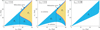Fig. 10 Stability of the coplanar equilibria in the (ψ⋆0, ψ1⋆) space for ϵ⋆p = 5.0, 2.0, and 0.99, respectively. The stable solutions, indicated by λ2 < 0, are marked with blue points, while the unstable solutions, where λ2 > 0, are marked with yellow points. The bifurcation curve corresponding to each value of ϵ⋆p is also depicted.

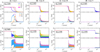Fig. 11 Dynamical evolution of multi-planet systems from Table 2. Each column displays the evolution of stellar obliquities and mutual planetary inclinations for a system under two distinct initial stellar obliquity angles (ψ⋆0). The magenta curves in each obliquity panel represent the evolution paths of equilibria. Note that in all simulations, we ignore the evolution of the eccentricity vectors by assuming all the orbits are initially circular. In addition to the parameters given in Table 2, other integration parameters are: m⋆ = 1M⊙, τd = 1 × 104 yr, rin = 0.03 au, and rout = 50 au. The disk mass (md) is set to 0.05M⊙ for Cases I-III and to 0.02M⊙ for Case V, respectively.

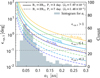Fig. 12 Estimations of ϵ⋆p,1 as a function of a1 for typical compact multi-planet systems. This figure displays estimations of ϵ⋆p,1 for three-planet systems with uniform planetary masses of m1-m3 = 5m⊕ and varying orbital separations δa = {16, 20, 25, 30} RH. Two sets of stellar parameters, resulting in J2 = 7.97 × 10−4 and J2 = 1.46 × 10−4, respectively, are adopted. The selection of δa= 16RH represents the minimum spacing required for these systems to maintain stability over 1 Gyr (Zhu & Dong 2021). The grade-shaded histogram (presented using the right y-axis) illustrates the distribution of a1 for the Kepler sample of multi-planet systems, which are retrieved from the NASA Exoplanet Archive.

Acknowledgements

This work was supported by the Fundamental Research Funds for the Central Universities.

References

All Tables

All Figures

Fig. 1 Geometric illustration of a multi-planet system with a misaligned protoplanetary disk. The disk’s angular momentum orientation is denoted by the unit vector ${\hat{\mathit{l}}}_{\mathrm{d}}$. The host star rotates at angular velocity Ω⋆ with its spin oriented along ${\hat{\mathit{s}}}_{\star }$. The primordial stellar obliquity (ψ⋆0) corresponds to the angle between ${\hat{\mathit{l}}}_{\mathrm{d}}$ and ${\hat{\mathit{s}}}_{\star }$. The angle between the planet’s orbit angular momentum vector (l1) and ${\hat{\mathit{s}}}_{\star }$ is referred to as the stellar obliquity (ψ1⋆).

In the text

Fig. 2 Coplanar equilibrium solutions and examples of orbital evolution using the full-space (nonlinear) disk gravity model (a) and the approximate linear model (b). The upper panels of (a) and (b) show equilibrium solutions as a function of ϵ⋆d (or ${ϵ}_{\star \mathrm{d}}^{\mathrm{\prime }}$) for ψ⋆0 = 70°. In (a), the coplanar equilibria (P2, P3, P4, and P5) and bifurcations (B1 and B2) are denoted. The lower panels of (a) and (b) show the evolution of the stellar obliquity through numerical integrations of corresponding secular equations. The dashed curves in the two panels represent the evolution of the equilibria.

In the text

Fig. 3 Phase portraits for ψ⋆0 = 70° and ϵ⋆d = 0.1 (a), 1.0 (b), and 10.0 (c) displayed on the unite sphere. These portraits were generated by plotting level curves of the perturbing Hamiltonian from Eq. (20) with |l1| = 1. The orientations of ${\hat{\mathit{s}}}_{\star }$ and ${\hat{\mathit{l}}}_{\mathrm{d}}$ are shown, along with the norm of the principal plane. Equilibria are marked by colored points, which correspond to the equilibrium solutions identified in Fig. 2a.

In the text

	Fig. 4 Values of f(ψ1⋆; ψ⋆0, ϵ⋆d) defined by Eq. (23) as functions of ψ1⋆ and ϵ⋆d for ψ⋆0 = 70°. The red and blue curves represent the critical ϵ⋆d that trigger the bifurcations B1 and B2, respectively, which are characterized by f = 0 and df/dψ1⋆ = 0. The two bifurcations are further distinguished by the sign of ${\mathrm{d}}^{2}f/\mathrm{d}{\psi }_{1\star }^2$: B1 (<0) and B2 (>0).
In the text

	Fig. 5 Bifurcation curves in the (ϵ⋆d, ψ⋆0) space obtained using the bifurcation conditions (Eq. (26)). Curves are shown for three disk softening scales: β = 0.01, 0.02, and 0.05. For β = 0.01, the bifurcation curves of B1 and B2 are in red and blue, respectively. Critical values of ψ⋆0 are also marked.
In the text

	Fig. 6 Stability of the circular coplanar equilibria as functions of ψ⋆0 and ψ1⋆ for ψ1⋆ ∈ (0, π/2), calculated using the stability condition, Eq. (32). Blue points represent stable equilibria where λ2 < 0, and yellow points indicate unstable equilibria where λ2 > 0. The red curve presents the bifurcation curve in the (ψ⋆0, ψ1⋆) space, derived from the bifurcation conditions (Eq. (26)).
In the text

Fig. 7 Phase portraits for ψ⋆0 = 70° presented in the (ψ1⋆ cos Δh, ψ1⋆ sin Δh) plane, where Δh represents the difference in the longitudes of the ascending node between the inner and outer orbits. These portraits were generated by plotting level curves of the perturbing Hamiltonian (Eq. (33)). In the upper panels, ϵ⋆p = 10.0 and ϵ⋆d = 0.1, 1.5, and 5.0, respectively. In the lower panels, ϵ⋆p = 1.0 with the same variations in ϵ⋆d. Equilibrium points are indicated with colored markers. The projections of ${\hat{\mathit{s}}}_{\star }$ and ${\hat{\mathit{l}}}_{\mathrm{d}}$ on this plane are denoted by filled triangles.

In the text

	Fig. 8 Bifurcation curves for hierarchical systems. (a) Bifurcation curves for several high values of ψ⋆0 presented in the (ϵ⋆d, ϵ⋆p) space. The dashed and solid curves represent the bifurcations B1 and B2, respectively. (b) Bifurcation curves in the (ψ⋆0, ϵ⋆p) space, where the curves for B1 and B2 degenerate into one curve. The softening scale is chosen as β = 0.01.
In the text

Fig. 9 Evolution of orbital inclinations between inner and outer orbits for hierarchical three-body systems obtained by integrating the secular equations for circular orbits. The system parameters are detailed in Table 1. We set the timescale of the disk dissipation (τd) to 1 × 104 yr. In (a), the decay of host stellar oblateness is not considered. In (b), the oblateness of the host star decays due to its radius contraction: R⋆ = R⋆ (0)/(1 + t/τR⋆)−1/3, where τR⋆ = 1 Myr. The temporal evolution of the equilibrium that dominates the planet’s evolution is depicted for each system. Notably, a jump in the equilibrium trajectory signifies an encounter with bifurcation B2.

In the text

	Fig. 10 Stability of the coplanar equilibria in the (ψ⋆0, ψ1⋆) space for ϵ⋆p = 5.0, 2.0, and 0.99, respectively. The stable solutions, indicated by λ2 < 0, are marked with blue points, while the unstable solutions, where λ2 > 0, are marked with yellow points. The bifurcation curve corresponding to each value of ϵ⋆p is also depicted.
In the text

Fig. 11 Dynamical evolution of multi-planet systems from Table 2. Each column displays the evolution of stellar obliquities and mutual planetary inclinations for a system under two distinct initial stellar obliquity angles (ψ⋆0). The magenta curves in each obliquity panel represent the evolution paths of equilibria. Note that in all simulations, we ignore the evolution of the eccentricity vectors by assuming all the orbits are initially circular. In addition to the parameters given in Table 2, other integration parameters are: m⋆ = 1M⊙, τd = 1 × 104 yr, rin = 0.03 au, and rout = 50 au. The disk mass (md) is set to 0.05M⊙ for Cases I-III and to 0.02M⊙ for Case V, respectively.

In the text

Fig. 12 Estimations of ϵ⋆p,1 as a function of a1 for typical compact multi-planet systems. This figure displays estimations of ϵ⋆p,1 for three-planet systems with uniform planetary masses of m1-m3 = 5m⊕ and varying orbital separations δa = {16, 20, 25, 30} RH. Two sets of stellar parameters, resulting in J2 = 7.97 × 10−4 and J2 = 1.46 × 10−4, respectively, are adopted. The selection of δa= 16RH represents the minimum spacing required for these systems to maintain stability over 1 Gyr (Zhu & Dong 2021). The grade-shaded histogram (presented using the right y-axis) illustrates the distribution of a1 for the Kepler sample of multi-planet systems, which are retrieved from the NASA Exoplanet Archive.

In the text

References

- Alexander, R., Pascucci, I., Andrews, S., Armitage, P., & Cieza, L. 2014, in Protostars and planets VI, eds. B. Henrik, K. Ralf S., P. D. Cornelis, & H. Thomas, 475 [Google Scholar]
- Alexander, R. D., Clarke, C., & Pringle, J. 2006, MNRAS, 369, 229 [NASA ADS] [CrossRef] [Google Scholar]
- Barber, M. G., Mann, A. W., Vanderburg, A., et al. 2024, Nature, 635, 574 [NASA ADS] [CrossRef] [Google Scholar]
- Bate, M., Lodato, G., & Pringle, J. 2010, MNRAS, 401, 1505 [NASA ADS] [CrossRef] [Google Scholar]
- Batygin, K. 2012, Nature, 491, 418 [NASA ADS] [CrossRef] [Google Scholar]
- Batygin, K., & Adams, F. C. 2013, ApJ, 778, 169 [NASA ADS] [CrossRef] [Google Scholar]
- Beaugé, C., & Nesvornỳ, D. 2012, ApJ, 751, 119 [CrossRef] [Google Scholar]
- Bourrier, V., Deline, A., Krenn, A., et al. 2022, A&A, 668, A31 [NASA ADS] [CrossRef] [EDP Sciences] [Google Scholar]
- Bouvier, J., Matt, S. P., Mohanty, S., et al. 2014, in Protostars and planets VI, eds. B. Henrik, K. Ralf S., P. D. Cornelis, & H. Thomas, 94 [Google Scholar]
- Cuddeford, P. 1993, MNRAS, 262, 1076 [NASA ADS] [Google Scholar]
- Davies, C. L. 2019, MNRAS, 484, 1926 [NASA ADS] [CrossRef] [Google Scholar]
- Dawson, R. I., Murray-Clay, R. A., & Johnson, J. A. 2014, ApJ, 798, 66 [Google Scholar]
- Dong, J., & Foreman-Mackey, D. 2023, AJ, 166, 112 [NASA ADS] [CrossRef] [Google Scholar]
- Fabrycky, D., & Tremaine, S. 2007, ApJ, 669, 1298 [NASA ADS] [CrossRef] [Google Scholar]
- Fielding, D. B., McKee, C. F., Socrates, A., Cunningham, A. J., & Klein, R. I. 2015, MNRAS, 450, 3306 [NASA ADS] [CrossRef] [Google Scholar]
- Ford, E. B., & Rasio, F. A. 2008, ApJ, 686, 621 [Google Scholar]
- Foucart, F., & Lai, D. 2011, MNRAS, 412, 2799 [NASA ADS] [CrossRef] [Google Scholar]
- Fu, T., & Wang, Y. 2024, ApJ, 973, L43 [Google Scholar]
- Fu, T., Wang, Y., & Hu, W. 2025, ApJ, 989, L5 [Google Scholar]
- Hahn, J. M. 2003, ApJ, 595, 531 [NASA ADS] [CrossRef] [Google Scholar]
- Hjorth, M., Albrecht, S., Hirano, T., et al. 2021, PNAS, 118, e2017418118 [NASA ADS] [CrossRef] [Google Scholar]
- Hurt, S. A., & MacGregor, M. A. 2023, ApJ, 954, 10 [NASA ADS] [CrossRef] [Google Scholar]
- Kennedy, G. M., Matrà, L., Facchini, S., et al. 2019, Nat. Astron., 3, 230 [Google Scholar]
- Lai, D. 2014, MNRAS, 440, 3532 [NASA ADS] [CrossRef] [Google Scholar]
- Lai, D., Foucart, F., & Lin, D. N. 2011, MNRAS, 412, 2790 [NASA ADS] [CrossRef] [Google Scholar]
- McLaughlin, D. 1924, ApJ, 60, 22 [NASA ADS] [CrossRef] [Google Scholar]
- Mestel, L. 1963, MNRAS, 126, 553 [NASA ADS] [CrossRef] [Google Scholar]
- Millholland, S., & Batygin, K. 2019, ApJ, 876, 119 [Google Scholar]
- Nagasawa, M., Ida, S., & Bessho, T. 2008, ApJ, 678, 498 [NASA ADS] [CrossRef] [Google Scholar]
- Naoz, S., Farr, W. M., Lithwick, Y., Rasio, F. A., & Teyssandier, J. 2011, Nature, 473, 187 [NASA ADS] [CrossRef] [Google Scholar]
- Petrovich, C., Muñoz, D. J., Kratter, K. M., & Malhotra, R. 2020, ApJ, 902, L5 [NASA ADS] [CrossRef] [Google Scholar]
- Rosenthal, L. J., Knutson, H. A., Chachan, Y., et al. 2022, ApJS, 262, 1 [Google Scholar]
- Rossiter, R. 1924, ApJ, 60, 15 [NASA ADS] [CrossRef] [Google Scholar]
- Schulz, E. 2012, ApJ, 747, 106 [Google Scholar]
- Spalding, C., & Batygin, K. 2015, ApJ, 811, 82 [Google Scholar]
- Spalding, C., & Millholland, S. C. 2020, AJ, 160, 105 [NASA ADS] [CrossRef] [Google Scholar]
- Su, Y., & Lai, D. 2020, ApJ, 903, 7 [Google Scholar]
- Touma, J., Tremaine, S., & Kazandjian, M. 2009, MNRAS, 394, 1085 [NASA ADS] [CrossRef] [Google Scholar]
- Tremaine, S., Touma, J., & Namouni, F. 2009, AJ, 137, 3706 [Google Scholar]
- Vick, M., Su, Y., & Lai, D. 2023, ApJ, 943, L13 [NASA ADS] [CrossRef] [Google Scholar]
- Wang, Y., & Fu, T. 2020, MNRAS, 495, 3307 [Google Scholar]
- Ward, W. R. 1981, Icarus, 47, 234 [NASA ADS] [CrossRef] [Google Scholar]
- Winn, J. N., Fabrycky, D., Albrecht, S., & Johnson, J. A. 2010, ApJ, 718, L145 [Google Scholar]
- Wu, Y., & Lithwick, Y. 2011, ApJ, 735, 109 [Google Scholar]
- Wu, Y., & Murray, N. 2003, ApJ, 589, 605 [Google Scholar]
- Zanazzi, J., & Lai, D. 2018, MNRAS, 478, 835 [NASA ADS] [CrossRef] [Google Scholar]
- Zhu, W., & Dong, S. 2021, ARA&A, 59, 291 [NASA ADS] [CrossRef] [Google Scholar]
- Zink, J. K., & Howard, A. W. 2023, ApJ, 956, L29 [Google Scholar]