| Issue |
A&A
Volume 705, January 2026
|
|
|---|---|---|
| Article Number | A156 | |
| Number of page(s) | 16 | |
| Section | Extragalactic astronomy | |
| DOI | https://doi.org/10.1051/0004-6361/202556060 | |
| Published online | 16 January 2026 | |
Probing the disk-jet coupling in M 87
1
Institut für Theoretische Physik und Astrophysik, Universität Würzburg Emil-Fischer-Str. 31 D-97074 Würzburg, Germany
2
Institut für Theoretische Physik, Goethe Universität Max-von-Laue-Str. 1 D-60438 Frankfurt, Germany
3
Max-Planck-Institut für Radioastronomie Auf dem Hügel 69 D-53121 Bonn, Germany
4
Tsung-Dao Lee Institute, Shanghai Jiao Tong University 1 Lisuo Road Shanghai 201210, People’s Republic of China
5
School of Physics & Astronomy, Shanghai Jiao Tong University 800 Dongchuan Road Shanghai 200240, People’s Republic of China
6
Key Laboratory for Particle Physics, Astrophysics and Cosmology, Shanghai Key Laboratory for Particle Physics and Cosmology, Shanghai Jiao-Tong University 800 Dongchuan Road Shanghai 200240, People’s Republic of China
7
Mullard Space Science Laboratory, University College London Holmbury St. Mary Dorking Surrey RH5 6NT, UK
★ Corresponding authors: This email address is being protected from spambots. You need JavaScript enabled to view it.
; This email address is being protected from spambots. You need JavaScript enabled to view it.
Received:
23
June
2025
Accepted:
17
November
2025
Abstract
Context. Recent GMVA observations of M 87 at event horizon scales revealed a ring-like structure that is ∼50% larger at 86 GHz than the ring observed by the Event Horizon Telescope at 230 GHz.
Aims. We studied a possible origin of the increased ring size at 86 GHz and the role the nonthermal electron population plays in the observed event horizon scales.
Methods. We carried out 3D general relativistic magnetohydrodynamic simulations followed by radiative transfer calculations. We incorporated synchrotron emission from both thermal and nonthermal electrons into the calculations. To better compare our results to observations, we generated synthetic interferometric data adjusted to the properties of the observing arrays. We fit geometrical models to these data in Fourier space through Bayesian analysis to monitor the variable ring size and width over the simulated time span.
Results. We find that the 86 GHz ring is always larger than the 230 GHz ring, which can be explained by the increased synchrotron self-absorption at 86 GHz and the mixed emission from both the accretion disk and the jet footpoints, as well as flux arcs ejected from a magnetized disk. We find agreement with the observations, particularly within the error range of the observational value of M/D for M 87.
Conclusions. We show that state-of-the art 3D general relativistic magnetohydrodynamic simulations combined with thermal and nonthermal emitting particles can explain the observed frequency-dependent ring size in M 87. Importantly, we find that MAD events triggered in the accretion disk can significantly increase the lower-frequency ring sizes.
Key words: accretion / accretion disks / black hole physics / magnetohydrodynamics (MHD) / radiation mechanisms: non-thermal / radiative transfer
© The Authors 2026
 Open Access article, published by EDP Sciences, under the terms of the Creative Commons Attribution License (https://creativecommons.org/licenses/by/4.0), which permits unrestricted use, distribution, and reproduction in any medium, provided the original work is properly cited.
This article is published in open access under the Subscribe to Open model. This email address is being protected from spambots. You need JavaScript enabled to view it. to support open access publication.
1. Introduction
General relativity predicts that event horizons exist generically in black holes, regardless of geometry (Penrose 1965). Lynden-Bell (1969) proposed that supermassive black holes (SMBHs) could explain some of the observables at the center of galaxies, an idea later supported by measurements of stellar and gas dynamics in nearby galaxies (Kormendy & Richstone 1995). Most galaxies are now believed to contain an accreting SMBH capable of launching a relativistic jet that is observable at subparsec to megaparsec scales (Blandford et al. 2019). These objects, known as active galactic nuclei (AGNs), are able to outshine their host galaxy.
Due to its proximity and bright jet, the elliptical galaxy M 87 provides an ideal laboratory for studying accretion and jet launching around SMBHs. M 87 appears on the sky as a bright, compact radio source, a characteristic feature of low-luminosity AGNs (Nagar et al. 2005). Di Matteo et al. (2003) furthermore estimated that the accretion of matter onto the central SMBH of M 87 is radiatively inefficient, and low-luminosity AGNs are often modeled through advection-dominated accretion flow models (Narayan & Yi 1995; Yuan & Narayan 2014). These systems describe accretion through an optically thin, geometrically thick torus, the “disk”, where most of the viscously dissipated energy is advected rather than radiated away, resulting in a luminosity lower than expected. Yuan et al. (2002) first proposed a disk-jet setup to explain the spectrum of a prototypical low-luminosity AGN at low frequencies.
The jet of M 87 was first observed at optical frequencies by Curtis (1918) and has since been extensively studied at wavelengths from the radio to γ-rays (Abramowski et al. 2012; MAGIC Collaboration 2020). Very long-baseline interferometry (VLBI) observations at millimeter wavelengths of the innermost core regions of M 87, 7 − 100 RS (where RS = 2GM/c2 is defined by the speed of light, c, the gravitational constant, G, and the mass of the black hole, M), show a limb-brightened jet with a wide opening angle and parabolic collimation, supporting the picture of a jet launched magnetically around a black hole (Reid et al. 1989; Junor et al. 1999; Hada et al. 2016; Mertens et al. 2016; Kim et al. 2018; Walker et al. 2018). The apparent position of the radio core shifts upstream with increasing frequency, indicating that the core is becoming optically thin to synchrotron emission. Hada et al. (2011) studied the core shift of M 87 and determined that the black hole overlaps with the observed radio core at frequencies ≥43 GHz, as the peak brightness should coincide with the position of the central engine (Blandford & Königl 1979).
Millimeter and submillimeter VLBI allows us to directly image the event horizon scales of AGNs, where the central SMBHs are expected to cast a shadow (Falcke et al. 2000). Only Sgr A★ and M 87 have an angular size large enough to be resolved by our current submillimeter VLBI technology. The event horizon region of M 87 was first resolved at 230 GHz by the Event Horizon Telescope (EHT), which found an asymmetric ring-like structure with a diameter of 42 ± 3 μas and a central depression. This morphology is consistent with the theoretical models of accretion onto a rotating black hole and remains present in more recent observations (Event Horizon Telescope Collaboration 2019a, 2024). Observations of Sgr A★ by the EHT provided further evidence in favor of the SMBH picture (Event Horizon Telescope Collaboration 2022a), but unlike Sgr A★, M 87 hosts a powerful, extended jet. Due to this, M 87 remains the only source for which we can hope to simultaneously resolve the extended jet and the event horizon structures. This was achieved by Lu et al. (2023) with 86 GHz observations by the Global Millimeter VLBI Array (GMVA) together with the Atacama Large Millimeter/submillimeter Array (ALMA) and the Greenland Telescope (GLT). They found a ring-like structure with a diameter (d) of  as, which is ∼50% larger than that at 230 GHz. More recently, Kim et al. (2025) applied two novel imaging algorithms to the 86 GHz data and found lower, but compatible, diameter values of 60.9 ± 2.2 μas and 61.0 μas.
General relativistic magnetohydrodynamic (GRMHD) simulations can model accretion onto a black hole and the subsequent jet launching. Coupled with general relativistic radiative transfer (GRRT) calculations that account for synchrotron emission, we can obtain synthetic images that can be compared to VLBI observations. The EHT Collaboration extensively studied which disk-jet setups could explain the observed intensity and polarization images at 230 GHz (Event Horizon Telescope Collaboration 2019d, 2021). They find that only models with strongly magnetized disks, known as magnetically arrested disks (MADs), remain viable, but that several values of the black hole spin (a*) can explain the observed polarization patterns.
Lu et al. (2023) also carried out 2D MAD simulations with a prograde black hole spin of 0.9, consistent with the modeling of the EHT. Through synchrotron GRRT calculations, they generated images at both 86 GHz and 230 GHz and from two different electron populations. They find that the diameter of the ring produced by non-thermally distributed (power-law) electrons is too small by at least 30% compared to the observational value, while thermally distributed (Maxwell-Jüttner) electrons produce rings with diameters consistent with observations at both frequencies.
In this work we modeled the event horizon and extended jet structure of M 87 at submillimeter frequencies by combining GRMHD simulations and GRRT, exploring the impact of a mixed distribution of thermal and nonthermal electrons. In Sect. 2 we introduce our GRMHD setup. In Sect. 3 we characterize the GRRT calculations that we carried out to obtain our synthetic images. In Sect. 4 we show and analyze the output of our simulations. We not only study our data in the image plane but also focus on generating synthetic interferometric data to take the limited resolution of real observations into account. Finally, we discuss our results in Sect. 5. Throughout this work, we assumed a black hole mass (mBH) of 6.5 × 10⁹ M⊙ and a luminosity distance (dL) of 16.5 Mpc. With these we computed the gravitational radius and time, which scale the dimensionless simulation output, 1 rg = GmBH/dLc2 = 3.8 μas and 1 tg = GmBH/c3 = 8.5 h.
2. GRMHD simulations
We simulated the accretion onto a rotating Kerr black hole with spin a★ = −0.5 and its associated jet launching with the 3D GRMHD code BHAC (Porth et al. 2017; Olivares et al. 2019). Our choice of black hole spin was motivated by modeling studies of the linear polarization data of M 87, wherein Event Horizon Telescope Collaboration (2021) found that MAD models with a★ = −0.5 met their scoring-based criteria more than any other combination of parameters. Our simulation follows the same setup as Fromm et al. (2022), but we give a brief summary below.
BHAC solves the equations of conservation of mass, conservation of energy-momentum, and the covariant Maxwell equations. We followed ideal, non-resistive magnetohydrodynamics, for which the stress-energy tensor takes the form
 (1)
(1)
Here, ρ is the rest-mass density, p is the gas pressure, htot = h + b2/ρ is the total specific enthalpy, uμ is the four-velocity, gμν is the space-time four-metric and bμ is the magnetic field four-vector. The specific enthalpy is computed by assuming an ideal gas equation of state,
 (2)
(2)
where  is the adiabatic index. Throughout this work we used an adiabatic index of
  . This value was chosen for the sake of consistency with recent BHAC simulations used by the EHT to model M 87 (Event Horizon Telescope Collaboration 2025). While this value results in more numerically robust simulations, two-temperature fluid simulations (Chael 2025) as well as theoretical works based on thermodynamic principles (Gammie 2025) find that a value closer to 5/3 may be more appropriate to model single-fluid simulations. We defined the magnetization as σ = b2/ρ and the plasma beta as β = 2p/b2, calculated through the square of the magnetic field:
 (3)
(3)
Here, the Latin index i refers only to the three spatial coordinates. Γ is the Lorentz factor of the fluid, and B2 = BiBi, where Bi is the three-vector of the magnetic field. Throughout this work we set G = c = 1 and employed spherical Kerr-Schild coordinates, (r, θ, ϕ). The outer radial edge of the simulation is located at r = 2500 M, and the inner one at 1.18rEH M, where  is the radius of the event horizon. Furthermore, we made use of three adaptive mesh refinement levels, which led to an effective resolution of 384 × 192 × 192 cells in the r, θ, and ϕ directions.
The initial setup of our simulations consists of a Fishbone-Moncrief torus (Fishbone & Moncrief 1976) in hydrostatic equilibrium characterized by its inner edge, rin = 20 M, the location of the pressure maximum, rc = 40 M and its specific angular momentum, l = −uϕ/ut = 6.88. This torus is seeded with a weak poloidal magnetic field given by the vector potential,
 (4)
(4)
and normalized to a plasma beta of β = 100 at rin.
The initial hydrostatic equilibrium is perturbed by a small pressure variation that triggers the formation of the magnetorotational instability, kick-starting the accretion. During the course of the simulation up to t = 30 000 M, we monitored the mass accretion rate (Ṁ) and the accreted magnetic flux, ϕBH. These were evaluated at the event horizon and defined as
 (5)
(5)
 (6)
(6)
Figure 1 showcases our initial setup and its evolution over time. The six panels on top display density maps of the centralmost region of our simulation. The top and bottom row of images display the equatorial and a meridional plane, respectively, at three different times during the course of the simulation. The leftmost panels show the density shortly after the start of the simulation, when the accretion process is not yet fully established, evidenced by the low-density gap between the central black hole and the high density innermost region of the torus. The two advanced time steps show both the accretion onto the black hole and the launching of a jet and a counter-jet, which are seen as low density funnels in the meridional plane. The central column shows a low density arc of matter being ejected from the direct vicinity of the black hole, a common event in MADs and one of their characteristic features. During these MAD events, the accumulated magnetic pressure pushes part of the disk outward, leading to low-density and highly magnetized regions known as MAD bubbles, which are then sheared out in the accretion flow and disappear. The bottom panels show the evolution of the mass accretion rate (Ṁ) and the MAD parameter,  . The latter oscillates around a value of 10, indicating that a MAD state has been reached as defined by Tchekhovskoy et al. (2011).
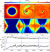 |
Fig. 1. Evolution of our GRMHD simulation over time. The top and middle panels show the logarithm of the density in the equatorial and a meridional plane, respectively, for three different times. The bottom panel shows the temporal evolution of the mass accretion rate (Ṁ) and the MAD parameter, |
3. Radiative transfer
We carried out the radiative transfer calculations with the GRRT code BHOSS (Younsi et al. 2012, 2016, 2020). The output of BHAC is straightforwardly used as input for the post-processing code BHOSS, which solves the equations of covariant GRRT,
 (7)
(7)
 (8)
(8)
alongside the affine parameter λ in environments with a strong gravity. Here the optical depth is defined as τν = ∫αν dλ, where αν is the absorption coefficient (or absorptivity) of the plasma that comprises the medium. jν is the emission coefficient (or emissivity) of the plasma and the subscript 0 indicates that it is the value in its local rest frame. The energy shift with respect to the observer’s frame is defined as γ−1 = ν0/ν, and the Lorentz-invariant intensity ℐ is related to the specific intensity Iν as ℐ = Iν/ν3.
We largely followed the same method as Fromm et al. (2022), where the GRRT calculations are explained in more detail, but we give here a summary for the sake of completeness. As the power associated with synchrotron radiation depends on the particle mass as P ∝ m−2 (Rybicki & Lightman 1986), and me ≪ mp, the majority of the synchrotron emission comes from the electrons in the plasma. To calculate the absorption and emission coefficients of Eqs. 7 and 8, we needed to establish the properties of the electrons, whose distribution function will depend on the dimensionless electron temperature Θe = kTe/mec2.
The GRMHD simulations carried out in Sect. 2 are single-fluid simulations, and thus the resulting temperature is only that of the protons in the plasma. We calculated the electron temperature Θe from the proton temperature following the R-β model of Mościbrodzka et al. (2016),
 (9)
(9)
The ratio between proton and electron temperature is regulated by the plasma beta β, following the formula
 (10)
(10)
This model introduces the parameters Rlow and Rhigh, which regulate the temperature ratio in the regions where the gas pressure (disk) and the magnetic pressure (jet) dominate, respectively.
In this work we used a hybrid electron distribution function (eDF), consisting of a mixed thermal and nonthermal distribution. In this type of astrophysical scenario, electrons are expected to be accelerated to nonthermal distributions through mechanisms such as turbulence, magnetic reconnection, or shocks. Here, we parametrized the nonthermal electrons via a kappa distribution (Davelaar et al. 2019; Cruz-Osorio et al. 2022; Fromm et al. 2022; Zhang et al. 2024). The kappa eDF takes a thermal-like shape for particles with small electron Lorentz factors, Γe, but transitions to a nonthermal power-law tail for large Γe (for details, see Pandya et al. 2016). The kappa eDF is parametrized by the slope of its nonthermal tail, i.e., the kappa parameter, κ, and its width, w. Following Davelaar et al. (2019) we calculated w as
![Mathematical equation: $$ \begin{aligned} w=\frac{\kappa -3}{\kappa }\Theta _e + \frac{\epsilon }{2}\left[1+\tanh {\left(r-r_{\text{ inj}}\right)}\right]\frac{\kappa -3}{6\kappa }\frac{m_\text{ p}}{m_\text{ e}}\sigma . \end{aligned} $$](/articles/aa/full_html/2026/01/aa56060-25/aa56060-25-eq17.gif) (11)
(11)
We assumed that the energy in the kappa distribution is coupled to a thermal value, and we included some fraction (ϵ) of the magnetic energy. This additional energy mimics the acceleration of particles, for example via magnetic reconnection after some distance (rinj).
The value of the κ parameter needs to be evaluated everywhere in the plasma. Past works, such as Davelaar et al. (2018), found that a fixed value of κ could not simultaneously fit the known spectral energy distribution and spectral index values of Sgr A★. They initially fixed this by reducing the number of accelerated electrons through an additional free parameter, a nonthermal/thermal electron fraction. Davelaar et al. (2019) improved on the model for M 87, parameterizing electron acceleration from first principles through the results from the particle-in-cell relativistic reconnection simulations of Ball et al. (2018, see also Sect. 4.2. of Event Horizon Telescope Collaboration 2022b). We used the same model of electron acceleration in our work. Ball et al. (2018) fit the electron power-law slope to the plasma beta and magnetization and obtained the analytical expression
 (12)
(12)
Based on the calculations of Pandya et al. (2016) for the relative fitting errors of the kappa distribution, we restricted our interval to 3 < κ ≤ 8. Up until this point, the GRRT calculations followed those of Fromm et al. (2022), which computed the emission and absorption coefficients following a kappa distribution within this range and a thermal distribution outside of it. We introduced a change in this step, still following the equations of Pandya et al. (2016) for the jν and αν coefficients. While we continued to use the coefficients of a thermal distribution, jν, thermal and αν, thermal, to carry out the GRRT calculations outside of our κ range, we introduced here a mixed efficiency model within the range
 (13)
(13)
The absorption coefficients are similarly computed, and the thermal and nonthermal contributions are distributed through a new magnetic efficiency parameter, ϵeff, following the equation
![Mathematical equation: $$ \begin{aligned} \tilde{\epsilon }=\epsilon _\text{ eff}\left[1-e^{-1/\beta ^2}\right]\left[1-e^{-\left(\sigma /\sigma _\text{ min}\right)^2}\right]. \end{aligned} $$](/articles/aa/full_html/2026/01/aa56060-25/aa56060-25-eq20.gif) (14)
(14)
As the initial ambient medium of our simulations is unmagnetized, and a large fraction of it will remain unmagnetized over the course of the simulation, Eq. (14) would return not-a-number values in the GRRT calculations. To avoid these numerical issues, we introduced σmin as a small cutoff value, well below the initial magnetization of the torus. Appendix A contains a visual of the value that  takes on the disk and jet regions of our simulation.
Our final model leaves us with a large parameter space to study. While Fromm et al. (2022) carried out a careful study of the impact of these parameters on the image properties and spectra, in this study we fixed the parameters to the values given by Table 1. These were chosen for their ability to retrieve an extended jet structure and to fit the high-frequency part of the spectrum. Specifically, σcut is a cutoff value for the maximum magnetization that will be included in the GRRT. High magnetization values can be found in the funnel of the jet, but this region is known to be affected by the floor-model used to increase the stability of the code. We set σcut = 5 to exclude this region during the GRRT calculations. This value is larger than the standard value of 1 (Event Horizon Telescope Collaboration 2025), meaning our model includes more emission from the jet funnel than previous studies. Fromm et al. (2022) found that σcut ≥ 3 resulted in an increased jet width and in the presence of a central ridge, likely due to the previously mentioned floor-model, as more magnetized, hot plasma is being included in the jet sheath with increasing σcut. The mass accretion rate was calculated via a minimization process to match the total flux at 86 GHz to observational data, 0.8 Jy, as observed by Lu et al. (2023).
Parameters of the GRRT calculations in this paper.
4. Results
The GRRT simulations were carried out from t = 20 000 M to t = 29 990 M, with a cadence of tcad = 10 M ≈ 3.7 days. We computed the emission over a frequency range of 1 × 10⁹ Hz to 1 × 10¹⁵ Hz, spaced logarithmically into 50 bins. We then generated images from the 86 GHz and 230 GHz data in a 2048 × 2048 pixel grid covering 200 M. This corresponds to an angular size of around 760 μas using the black hole mass and distance of M 87. We used the fast-light approximation, ignoring the finite speed of light during the radiative transfer calculations.
The top panels of Fig. 2 show the output of our GRRT calculations at t = 26 000 M for 86 GHz and 230 GHz. The images are blurred with half of the nominal resolution of the GMVA and the EHT, indicated by the white circle at the bottom right. They are dominated by a bright central ring-like structure and display an edge-brightened jet. The bottom panel shows the broadband radio spectrum of M 87 alongside the spectrum obtained from our model (solid red line).
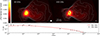 |
Fig. 2. Results of the GRRT calculations at t = 26 000 M. The images show the flux density at 86 GHz and 230 GHz. Notice that the images are convolved with half of the nominal resolution of the GMVA (27 μas) and the EHT (10 μas), indicated by the white circle at the bottom right. The contours begin at 1/1000 of the maximum flux density and increase by factors of two. In the bottom panel we display the broadband radio spectrum of our model. The observational flux values are taken from Prieto et al. (2016), Perlman et al. (2001), Whysong & Antonucci (2004), Hada et al. (2017), and Lister et al. (2018). |
In Fig. 3 we zoom into the horizon region of Fig. 2. We additionally decompose the image into the emission originating from the disk and from the jet, to better understand their contribution to the total image. For this purpose, during the GRRT calculations we set the emission coefficients to zero in either the jet or disk while keeping the absorption coefficients unchanged. We used the Bernoulli parameter −hut = 1.02 to separate the disk and jet, marking the transition between the bound gas of the disk and the unbound gas of the jet (Porth et al. 2019; Moriyama et al. 2024). The decomposition shows that the innermost region is dominated by emission from the disk, but there is some contribution from the jet foot-points at larger radii. It is interesting to remark that the bright spots seen in the disk and jet decompositions do not necessarily coincide, which indicates that on horizon scales we see the variability in both the accretion flow and in the jet formation zone. We provide further details and discussion on temporal variation in Sect. 5 and Appendix B.
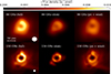 |
Fig. 3. Structural decomposition of the horizon scale structure in our model at t = 26 000 M. The panels show from left to right the total, disk, and jet plus wind contributions for 86 GHz (top row) and 230 GHz (bottom row). |
In order to compare our numerical results to observations, we computed synthetic visibilities from our images and perform the analysis in the Fourier plane. To do this, we used the ehtim package (Chael et al. 2018) to Fourier transform and sample all of our images with the baselines of real observations. This was done through the equation
 (15)
(15)
where a baseline formed by the (i, j) stations detects a complex visibility Vij. Figure 4 shows the u − v coverage used in this paper, comprising every (u, v) pair. We sampled every 86 GHz image with the baselines of Lu et al. (2023) and added the errors they calculated to the visibilities. We similarly produced synthetic visibilities for our one thousand 230 GHz images with the baselines of the 2017 observation of M 87 by the EHT 1. The stations that participated in both observations, and their respective sensitivities in system-equivalent flux density (SEFD), are given in Table 2. Throughout this paper we refer to the synthetic visibilities created from our GRMHD and GRRT models as “data.” However, our “data” should not be confused with real observational data of the GMVA and the EHT.
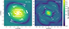 |
Fig. 4. Fourier transforms of the central regions of our simulated data at t = 24 500 M. Plotted on top is the u − v coverage at 86 GHz and 230 GHz used for the generation of synthetic observations, using the array configurations presented in Lu et al. (2023) and Event Horizon Telescope Collaboration (2019a), respectively. Note the different scales in the two plots. |
Antennas involved in the observations used to generate synthetic data and their nominal sensitivities.
We conducted our study of the ring morphology over two quantities: the visibility amplitudes and the closure phases. Closure phases were defined as the phase ψC of the product of three visibilities in a triangle formed by three stations,
 (16)
(16)
Being the product of a triangle of baselines makes closure phases robust to station-based calibration errors, making them useful in radio interferometry (Chael et al. 2018). Furthermore, nonzero closure phases are indicative of an azimuthally asymmetric structure, and have been observed for M 87 at 230 GHz (Event Horizon Telescope Collaboration 2019a). Indeed, modeling work done by the EHT supports the necessity of fitting azimuthally asymmetric models to the data (Event Horizon Telescope Collaboration 2019e).
It is relatively straightforward to fit symmetric models such as Gaussians, thin rings and disks to the data. The Fourier transforms of these geometries are proportional, respectively, to a Gaussian, a Bessel function of order zero and of order one. Furthermore, due to being real-valued everywhere, the closure phases can only take on the values of 0° or 180°. A thick ring, modeled by ehtim as a thin ring blurred by a Gaussian kernel, is similarly symmetric but may be able to successfully retrieve the underlying structures. Lu et al. (2023) fit all of these symmetric models to the 86 GHz, 14-15 April 2018 observation of M 87, and find a thick ring to be the best-suited model to fit the data and retrieve the ring diameter. While we used an asymmetric model to fit our data at both frequencies, as explained in the next section, we explore the performance of these symmetric models on our time-variable data in Appendix C.
4.1. 86 GHz fitting
The EHT used Bayesian evidence to evaluate in depth how different geometric models of increasing complexity fit 230 GHz M 87 data from 2017 and 2018 (Event Horizon Telescope Collaboration 2019e, 2024). They arrived at the conclusions that (i) ring-like models overall fit the data much better than non-ring models, with the best-performing non-ring model consisting of three elliptical Gaussians, and (ii) the symmetric models are the worst performers by several orders of magnitude. Their best performing models contain upward of 20 free parameters. Fitting models with this many degrees of freedom is challenging since they require robust bounds, which can be difficult to mantain over a large amount of time steps with a degree of variability that is unknown in advance, as is our case. We decided to use the model that contains the fewest degrees of freedom while still performing well: a thick m-ring with m = 2. This model is described in polar coordinates (r, ϕ) by the equation (see Johnson et al. 2020)
 (17)
(17)
Here, the first term containing the delta function is the expression for an infinitesimally thin ring of total flux F0 and diameter d. The exponential term corresponds to a Gaussian that blurs the ring and turns it into a thick ring of thickness α. Finally, the ring is modulated by a sum of Fourier modes with complex coefficients βk, not to be confused with the plasma beta. It is this term that confers an azimuthal structure to the ring, specifically up to a quadrupole in the case of our m = 2 model. The visibilities of the thick m-ring model are given by the Fourier transform of Eq. (17),
 (18)
(18)
Jk is the Bessel function of order k, while (u, ϕu) are the polar coordinates in the interferometric plane. The sum of m-modes distinguishes this model from symmetric ones, as this function is complex-valued and thus can have closure phases that are not 0° or 180° everywhere. This can be seen in the bottom panel of Fig. 5, which shows the closure phases of a model (red) fit to the data of a specific time step (gray). The nonzero closure phases in the long baselines are indicative of azimuthal structure, and they are successfully modeled by Eq. (18). The top panel, which shows the visibility amplitudes, also highlights the necessity of the last term in Eq. (18) to fit many of our time steps. The sum of Bessel functions can retrieve the structures observed in the middle and long baselines, where the same uv distance can contain several different values of the visibility amplitudes. This implies an asymmetry in the visibilities observed by baselines of similar length, pointing toward, for example, a north-south and east-west asymmetry.
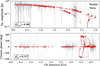 |
Fig. 5. Visibility amplitudes and closure phases over uv distance for the time step t = 28 600 M at 86 GHz. Overlaid in red is the result of fitting a thick m-ring model to the data. The χ2 values have been calculated taking an additional 10% error into account for ALMA visibilities. |
We carried out the fitting shown in Fig. 5 for all of our time steps at 86 GHz. We used the baseline and error information of Lu et al. (2023) to sample the Fourier transform of each of our images and, following their work, average the visibilities every 420 seconds. This operation was done on the central 100 μas of each image so as to not include the bulk of the extended jet emission in the dataset, as explained in Appendix E. To fit the resulting visibilities, we used the modeling capabilities of the Python package ehtim (Chael et al. 2016, 2018). We chose to use the minimizer function “dynamic nested sampling” of the dynesty package (Speagle 2020; Skilling et al. 2004; Skilling 2006; Higson et al. 2019). This evaluates the Bayesian evidence of a model and allows us to examine the final posteriors of the fit parameters. We show one set of such posteriors in Appendix B.
We evaluated the goodness of fit of our models to the data through the time-averaged mean squared residuals, χ2, for the amplitude and closure phases. The χ2 are computed as
 (19)
(19)
 (20)
(20)
To understand whether the thick m-ring model is adequate to fit our large dataset, we first ran a series of tests on a smaller subset of our data, which can be found in Appendix C. A weak fit will not retrieve reliable parameters from the data, as features such as the diameter or thickness of a ring are related to the nulls in the visibilities. We find that a thick m-ring model provides a reasonably good fit for most time steps, despite its relatively low number of degrees of freedom. We then used this m = 2 m-ring model for our larger 86 GHz dataset and added an error of 10% of the visibility amplitude to ALMA visibilities. The GMVA together with ALMA and the GLT comprise a heterogeneous array, with ALMA data having a much higher signal-to-noise ratio than other stations. Thus, adding a fractional error to the visibilities of those baselines aids in the convergence of the fitting routine, which would be otherwise dominated by the small error bars of ALMA data. This adjustment of ALMA uncertainties has been used on the 230 GHz EHT observations (Event Horizon Telescope Collaboration 2019c, 2024). Event Horizon Telescope Collaboration (2019c) tests adjusting the weights of ALMA visibilities to values between 0.01 and 1.0 with a similar motivation of avoiding data from these baselines dominating the phase and amplitude correction. For the 2017 230 GHz data, this would correspond to an added fractional error of 0%−40% of the visibility amplitudes. We find that for our 86 GHz data, a 10% error returns satisfactory results in aiding convergence without having ALMA data dominate the geometric fitting.
4.2. 230 GHz fitting
The 230 GHz visibilities were computed from the baselines and errors of Event Horizon Telescope Collaboration (2019a). The real April 2017 EHT observations had a variable error budget; the Large Millimeter Telescope (LMT) had a particularly high one due to poor amplitude calibration (see Event Horizon Telescope Collaboration 2019b). We assigned a 10% fractional error to all stations so as to not excessively down-weight any particular station.
We first carried out a study of the fitting models on a smaller subset of data, in the same time range as the one chosen for 86 GHz. We found that the m = 2 m-ring could not satisfactorily fit the visibilities at 230 GHz, and decide on a more complex geometric model. Following the example of Event Horizon Telescope Collaboration (2019e, 2022a), we added two asymmetric Gaussians, with free major and minor full widths at half maximum, position angle, flux, and (x, y) coordinates. This raises the number of parameters from 7 to 19. These free Gaussians can model generic features of the emission surrounding the central ring, which becomes distinct due to the decreasing optical thickness. More information can be found in Appendix D. We increased the field of view (FOV) to 140 μas to compute the visibilities. We find this change does not significantly affect the diameter or thickness retrieved from the model fitting, unlike the 86 GHz case, as shown in Appendix E. However, the increased FOV reduced the clipping of the Gaussian features out of frame, helping better locate their centroids.
5. Discussion
5.1. Ring size
We show the distribution of diameters resulting from applying the fitting procedure to all one thousand of our time steps in Fig. 6. We provide the information pertaining to the total flux and ring thickness in Appendix B.
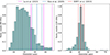 |
Fig. 6. Normalized distribution of the diameters resulting from fitting our models to the 86 GHz and 230 GHz datasets. The other parameters can be found in Appendix B. The vertical lines show the central observational values (solid) as well as upper and lower range (dashed) of the ring diameter at both frequencies. We use the range found by Event Horizon Telescope Collaboration (2019a) at 230 GHz. At 86 GHz, we plot the range found by Lu et al. (2023) and the range found by Kim et al. (2025) using the resolve algorithm. |
We calculated mean values of 55.0 ± 3.7 μas for the 86 GHz ring and 41.4 ± 4.9 μas for the 230 GHz ring. Using the median values, and the distance to the Q1 and Q3 quartiles as lower and upper errors, we calculated  as at 86 GHz and
  as at 230 GHz. While the 230 GHz distribution is strongly peaked, the higher number of degrees of freedom in the model result in more outliers, which affects the standard deviation. We use the median and interquartile values in the rest of the paper.
Up until here, we carried out our fitting procedure on GRRT data where the black hole mass and distance to us had the central values of mBH = 6.5 × 10⁹ M⊙ and dL = 16.5 Mpc, respectively. This matches the central value of angular gravitational radius estimated by Event Horizon Telescope Collaboration (2019a), GM/Dc2 = 3.8 ± 0.4 μas.
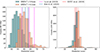 |
Fig. 7. Distribution of the diameters resulting from fitting our models to the 86 GHz and 230 GHz datasets. The turquoise and orange histograms show, respectively, the result of model fitting to GRRT data with an angular scale of 3.8 μas and 4.2 μas. The vertical lines show the observational range for the diameter of the ring, using the same values as Fig. 6. |
We repeated our fitting procedure taking into account this 0.4 μas uncertainty in our current values for the mass of the M 87 black hole and its distance to us. We incorporated this ≈10% error in the angular size of our image, increasing it to match the GM/Dc2 = 4.2 μas value and repeating the analysis to estimate an upper bound for our parameters. Increasing the FOV to match the angular size, we find the new fittings to be largely consistent with the old ones in the image plane, as expected. The GM/Dc2 = 4.2 μas data yield median diameters of  as at 86 GHz and
  as at 230 GHz. While the latter is on the upper error range of the observational value observed by the EHT, 42 ± 3 μas, this shows the impact on the ring size of the uncertainties in the angular scale, that is, in the mass and distance of the black hole.
While the GRRT images computed at 86 GHz with an angular scale of 4.2 μas produce a median ring size closer to the central observational values of  as and 60.9 ± 2.2 μas, the upper bound of
  as from the 3.8 μas images overlaps with the lower bounds of the observational value of Lu et al. (2023). Even at this angular scale, a significant number of time steps appear to fall within the error range of the observed values, as seen in Fig. 6. We find diameters that fall within the observational range of Lu et al. (2023) for around one third of the time steps. We explore the nature of these in Sect. 5.3.
5.2. Azimuthal structure
Figure 8 shows the distribution of the two beta modes resulting from fitting our model to the entire 86 GHz dataset. Note that due to the symmetry of the quadrupole mode, arg(β2) is ambiguous by 180°.
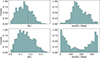 |
Fig. 8. Normalized distribution of the absolute values and argument for the m = 1, 2 beta modes resulting from the model fitting of the 86 GHz data. |
The resulting azimuthal structure of a given time step will depend not only on the position of the m = 1 and 2 beta modes of Eq. (18), corresponding respectively to a dipole and quadrupole mode, but also on their absolute value relative to each other. In a time step where |β1| ≫ |β2|, the structure will take on the shape of a crescent-like structure, with the brightest regions located in the position of arg(β1). Inversely, if |β1| ≪ |β2|, the emission will be dominated by a quadrupole structure with two hotspots opposite of each other. If both absolute values are nearly zero, the central region will present a nearly symmetrical ring-like shape. Finally, if the two modes have comparable absolute values, the source will present a more complex structure, dependant on the relative position of the angles. This is showcased in Fig. 9. Note that the bottom right image displays a similar structure to that observed by Lu et al. (2023).
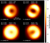 |
Fig. 9. Four time steps that display different ring morphologies (clockwise from the top left): dipole-dominant, quadrupole-dominant, complex, and ring-like. The more complex structure is caused by nonzero beta modes that are comparable in magnitude. |
While the 230 GHz data follow the same logic, analyzing the physical meaning of the beta modes is less straightforward due to the extra degrees of freedom in our model and the effect of the free Gaussians on the ring morphology.
5.3. Role of nonthermal emission and magnetic flux eruption events
Figure 10 shows the 230 GHz and 86 GHz image structure at 29 800 M, where each plot is normalized to its maximum flux. The GRRT images and their corresponding parametrized models have both been blurred with the same beam for each frequency. The increased resolution of 230 GHz observations allows for the surrounding emission to be separated from the underlying ring, while these elements blend together at 86 GHz, resulting in a ring of larger apparent diameter. At the same time, the non-blurred GRRT images show the additional effect of optical depth at these frequencies. The surrounding emission becomes fainter at 230 GHz, while it could be a significant contribution to the overall morphology at 86 GHz.
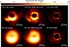 |
Fig. 10. Comparison of the underlying GRRT data and the output of our model fitting at 230 GHz (top) and 86 GHz (bottom) for t = 29 800 M. Right column: Output of the GRRT calculations, non-blurred. Central column: Same GRRT images, blurred by a beam of 10 μas and 27 μas for 230 GHz and 86 GHz, respectively. Left column: Parametrized model resulting from our fitting procedure, blurred with those same beams. All plots have been normalized to their maximum flux for ease of comparison. Note the increased surrounding flux at 86 GHz in the right column. |
To investigate these effects, we focused on one of the time steps with a diameter that fell within the observational values, t = 24 000 M, with a diameter of 60.3 ± 0.3 μas. In the upper limit of GM/Dc2 = 4.2 μas, this increased to 64.9 ± 0.3 μas. The data at the central GM/Dc2 value, as seen in Fig. 6, contains diameters that fall within the range calculated by Lu et al. (2023) for 36% of the time steps, and for the narrower range calculated with resolve by Kim et al. (2025) for 12%. For the upper GM/Dc2 limit, seen in Fig. 7, this respectively becomes 86% and 43% of the time steps.
To examine the cause of this, Fig. 11 shows spectral information at the central 200 μas for t = 24 000 M. We computed these maps with logarithmically spaced frequencies between 100 MHz and 500 GHz using 100 bins. The leftmost plot shows the turnover frequency at which the emission becomes optically thin. The central plot shows the flux density at this frequency. The rightmost plot shows the spectral index between the turnover frequency and 500 GHz.
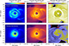 |
Fig. 11. Distribution of the turnover frequency, turnover flux density, and optically thin spectral index for a mixed eDF of thermal and kappa distribution (top) and thermal eDF only (bottom) at t = 24 000 M. |
The upper row of Fig. 11 shows our usual GRRT calculations, with a mix of thermal and nonthermal electrons as modeled by a κ distribution. The leftmost plot shows turnover frequencies of ∼50 − 60 GHz within a radius of r ∼ 50 μas. Most of the flux is distributed roughly within the same radius, as seen in the turnover flux density plot in the middle panel. Interestingly, the optically thin spectral index is steep, ∼ − 0.5, within r ∼ 30 − 40 μas while a flat value of ∼0 is obtained outside. Note that we injected nonthermal particles at a distance of rinj = 10 M = 38 μas, which explains the flattening of the spectral index on larger distances due to the power-law tail of the kappa distribution and our choice of the kappa parameter (see Eq. (12)).
Using this time step as a laboratory, we reran our GRRT calculations on the same GRMHD data, this time only computing the emission and absorption coefficients of a purely thermal electron distribution, that is, assuming the emission to be thermal everywhere. The effects of this on the spectral profile of the t = 24 000 M data are seen in the bottom row of Fig. 11. The turnover frequencies of ≈60 GHz are now concentrated within r ∼ 40 μas, and are lower outside of that. Changing the eDF has a less apparent impact on the turnover flux density maps, compared to the turnover frequency maps. This is not a surprise, as the kappa-eDF shares the core of the thermal eDF, i.e., most of the emission is still generated by the thermal particles. The most severe differences occur in the optically thin spectral index, especially outside of r ∼ 30 − 40 μas, where it takes on a value of around −1.0, in agreement with the exponential decay of the thermal emissivity jν, th ∝ exp( − ν). These dramatic differences support our conclusion: a combination of a lower turnover frequency in the outer areas of the ring as well as a much steeper spectral index would result in a smaller ring at 86 GHz in the thermal-only case, in contrast to the extended emission structure of the mixed eDF. We ran our thick m-ring fitting algorithm to the thermal-only t = 24 000 M data and found a ring diameter of 51.7 ± 0.4 μas, a significant decrease from 60.3 ± 0.3 μas, supporting our findings based on the spectral properties.
However, the question arises of which plasma events cause the extent of the flux in the emission region, how long do they last and how common are they. To examine this, we analyzed the plasma properties between 23 200 M and 24 400 M. In Fig. 12 we present the evolution over several time steps of the plasma and its associated emission in the equatorial planes. MAD simulations are known for frequent ejection events of magnetic flux emerging from a magnetically saturated black hole magnetosphere (see, e.g., Igumenshchev 2008). These manifest as bundles of poloidal magnetic field penetrating through low density blobs or arcs in the accretion flow of the disk. In our simulations, these blobs are best seen at t = 23 600 M (dark blue region). These regions shear out in the accretion flow (Porth et al. 2021) and are subject to particle acceleration via magnetic reconnection (see, e.g., Hakobyan et al. 2023). In addition, the accretion disk is commonly affected by Rayleigh-Taylor instabilities, which are capable of triggering magnetic reconnection at the intersection of the spiral-like accretion streams (Zhdankin et al. 2023). We selected these regions based on the criterion that  in Eq. (14), and plot them as black contours in the top panels of Fig. 12. In addition to the flux bundles (blue), we also see the shearing regions in the accretion flows (light green). The corresponding emission coefficients for both our hybrid thermal-nonthermal model and thermal-only model are shown in the two middle rows. Notice that we used the emission model presented in Table 1. A value of Rhigh = 160 will lead to a low electron temperature in the disk, resulting in only the innermost regions generating emission, as can be seen in the images. We furthermore applied a magnetization cutoff value of σcut = 5, rejecting emission from highly magnetized regions. This explains the missing emissivity in the orbiting flux bundles (dark regions within the bundles, best seen at t = 23 600 M) and the missing emissivity close to the black hole at t = 23 400 M. We see that the emitting region expands during the flux eruption event, independent from the choice of eDF. After t ∼ 800 M (∼280 days for M 87), the emitting region is back to a size similar to the one before the eruption event. The addition of nonthermal particles enhances the emissivity within the flux bundles and adds additional emissivity into the magnetized accretion streams (best seen at t = 23 800 M), explaining the increased ring diameter estimated for the nonthermal models compared to the thermal ones. This effect is intensified during the flux eruption events due to the aforementioned processes.
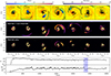 |
Fig. 12. Evolution of a MAD event in the equatorial plane. Top row: Logarithm of the density with overlaid contours indicating locations of particle acceleration, where |


Examining the evolution of the MAD parameters in Figs. 1 and 12 shows that our selected time step of t = 24 000 M displays a strong depression in the MAD parameter, following a large peak. Before this event, but after the initial stabilization of the accretion, the MAD parameter evolved in peaks and valleys in a quasi-periodical fashion around a stable value. After the large peak at t = 23 280 M and following depression, accretion appears perturbed. The average value of the MAD parameter decreases, and so does its variance. The central column of Fig. 1 and many of the columns in Fig. 12 show an “active” state where MAD bubbles appear, in which electron acceleration takes place resulting in emission further away from the central disk. Meanwhile, the rightmost columns of both plots show a “quiescent” state, where these features cannot be found and we expect to retrieve the underlying, smaller ring. To examine this assumption, we split the data shown in Fig. 6 before and after this t = 24 000 M depression in the MAD parameter, and plotted the results in Fig. 13. Indeed, while still larger than the 230 GHz diameters, the near entirety of the 86 GHz data after t = 24 000 M falls outside of the observational ranges, while 75% of the data before this time falls inside the range of Lu et al. (2023). Critically, the 230 GHz data do not appear affected by splitting the data in this way: while the 86 GHz data have a median diameter of  as before t = 24 000 M and
  as after, 230 GHz yields
  as and
  as, respectively. This backs our conclusion that the perceived ring size at 86 GHz is highly sensitive to both the nonthermal particle population and the underlying dynamics of the accretion disk.
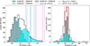 |
Fig. 13. Distribution of the diameters resulting from fitting our models to the 86 GHz and 230 GHz datasets. The data are the same as in Fig. 6, here shown split into the time steps before and after t = 24 000 M. The black outline shows the total distribution, corresponding to that of Fig. 6. The vertical lines show the observational range for the diameter of the ring, using the same values as Fig. 6. |
6. Summary and outlook
In this study we carried out 3D GRMHD jet launching simulations followed by GRRT calculations that incorporated a mixed emission model that took both thermal and nonthermal synchrotron emission into consideration. We studied one thousand time steps over a range of several years to be able to study the apparent change in ring size at 86 GHz in the context of jet launching variability. To provide a more robust analysis of our data, we Fourier-transformed and sampled them with the real observational data of Lu et al. (2023), who studied the source at 86 GHz and found a ring size ∼50% larger than that observed at 230 GHz by the EHT. We fit an azimuthally asymmetric thick m-ring model to our full visibility dataset and studied the distribution of the ring parameters, particularly focusing on the diameter. We carried out a similar analysis for our 230 GHz data, though with two free Gaussians added to the thick m-ring model to account for surrounding emission. We repeated our calculations to study the upper limits of the mass over distance ratio found by the EHT, GM/Dc2 = 4.2 μas. We finally studied the variability of the hotspots as well as the spectral profile of the source. Our main findings are as follows:
-
With the central value of mass over distance, GM/Dc2 = 3.8 μas, we find a median ring diameter of
 as at 86 GHz and
  as at 230 GHz. While the latter is in agreement with the observational value of 42 ± 3 μas, the former has a small overlap with the observational value of
  as.
as. -
The angular gravitational radius inferred by the EHT carries an uncertainty of ∼10%, GM/Dc2 = 3.8 ± 0.4 μas. Changing this parameter from 3.8 μas to 4.2 μas in our GRRT data and rerunning our fitting procedure yields a median diameter of
 as at 86 GHz and
  as at 230 GHz. The latter is still within the range observed by the EHT, and the former is now in close agreement with the observational values found by Lu et al. (2023) as well as, more recently, Kim et al. (2025).
 -
Strong MAD events can lead to a 86 GHz ring size in agreement with the observed one. In particular, we studied one of the time steps that matches the observations. Rerunning our GRRT calculations only accounting for thermal emission and examining the resulting spectral profile shows that producing this larger diameter is no longer possible. This indicates that the acceleration of electrons to nonthermal distributions may be necessary to explain the observed morphology of this source.
-
We focused on the evolution of the MAD parameter over time, as we find that our simulation contains a particularly powerful MAD event that disrupts accretion for an extended amount of time afterward. We find that the inherent variability of a jet launched by a MAD disk greatly impacts the perceived ring size. We specifically find that the size of the 86 GHz ring in our hybrid eDF model is affected by MAD events and an eruption of magnetic flux arcs, which can significantly increase the ring size.
-
Finally, we briefly studied how the variability of both the accreting disk and the jet footpoints impacts the morphology of the ring at 86 GHz. Depending on the state of the source, the central structure could be ring-like, crescent-like, quadrupole-like, or have a more complex structure.
Future work will focus on improving the nonthermal model, for example by including the effect of electron heating via turbulence or magnetic reconnection. Furthermore, incorporating polarized emission into our GRRT calculations will allow us to further constrain the nature of the 86 GHz ring and to better understand the importance of nonthermal particles, as different eDFs affect emissivities, absorptivities, and rotativities in all polarization channels. We further intend to explore the capabilities of future arrays, such as the ngEHT and the ngVLA, and their role in better understanding the physics of jet-disk coupling.
Acknowledgments
This research is supported by the DFG research grant “Jet physics on horizon scales and beyond” (Grant No. 443220636) within the DFG research unit “Relativistic Jets in Active Galaxies” (FOR 5195). The numerical simulations and calculations have been performed on MISTRAL at the Chair of Astronomy at the JMU Wuerzburg and on iboga at the Institute for theoretical physics in Frankfurt. YM is supported by the National Key R&D Program of China (grant no. 2023YFE0101200), the National Natural Science Foundation of China (grant no. 12273022), and the Shanghai municipality orientation program of basic research for international scientists (grant no. 22JC1410600). This research is supported in part also by the ERC Advanced Grant “JETSET: Launching, propagation and emission of relativistic jets from binary mergers and across mass scales” (grant No. 884631)
References
- Abramowski, A., Acero, F., Aharonian, F., et al. 2012, ApJ, 746, 151 [NASA ADS] [CrossRef] [Google Scholar]
- Ball, D., Sironi, L., & Özel, F. 2018, ApJ, 862, 80 [Google Scholar]
- Blandford, R. D., & Königl, A. 1979, ApJ, 232, 34 [Google Scholar]
- Blandford, R., Meier, D., & Readhead, A. 2019, ARA&A, 57, 467 [NASA ADS] [CrossRef] [Google Scholar]
- Chael, A. 2025, MNRAS, 537, 2496 [Google Scholar]
- Chael, A. A., Johnson, M. D., Narayan, R., et al. 2016, ApJ, 829, 11 [Google Scholar]
- Chael, A. A., Johnson, M. D., Bouman, K. L., et al. 2018, ApJ, 857, 23 [Google Scholar]
- Cruz-Osorio, A., Fromm, C. M., Mizuno, Y., et al. 2022, Nat. Astron., 6, 103 [NASA ADS] [CrossRef] [Google Scholar]
- Curtis, H. D. 1918, Pub. Lick Obs., 13, 9 [NASA ADS] [Google Scholar]
- Davelaar, J., Mościbrodzka, M., Bronzwaer, T., & Falcke, H. 2018, A&A, 612, A34 [NASA ADS] [CrossRef] [EDP Sciences] [Google Scholar]
- Davelaar, J., Olivares, H., Porth, O., et al. 2019, A&A, 632, A2 [NASA ADS] [CrossRef] [EDP Sciences] [Google Scholar]
- Di Matteo, T., Allen, S. W., Fabian, A. C., Wilson, A. S., & Young, A. J. 2003, ApJ, 582, 133 [NASA ADS] [CrossRef] [Google Scholar]
- Event Horizon Telescope Collaboration 2019a, ApJ, 875, L1 [Google Scholar]
- Event Horizon Telescope Collaboration 2019b, ApJ, 875, L3 [Google Scholar]
- Event Horizon Telescope Collaboration 2019c, ApJ, 875, L4 [CrossRef] [Google Scholar]
- Event Horizon Telescope Collaboration 2019d, ApJ, 875, L5 [NASA ADS] [CrossRef] [Google Scholar]
- Event Horizon Telescope Collaboration 2019e, ApJ, 875, L6 [NASA ADS] [CrossRef] [Google Scholar]
- Event Horizon Telescope Collaboration 2021, ApJ, 910, L13 [CrossRef] [Google Scholar]
- Event Horizon Telescope Collaboration 2022a, ApJ, 930, L12 [NASA ADS] [CrossRef] [Google Scholar]
- Event Horizon Telescope Collaboration (Akiyama, K., et al.) 2022b, ApJ, 930, L16 [NASA ADS] [CrossRef] [Google Scholar]
- Event Horizon Telescope Collaboration 2024, A&A, 681, A79 [NASA ADS] [CrossRef] [EDP Sciences] [Google Scholar]
- Event Horizon Telescope Collaboration 2025, A&A, 693, A265 [NASA ADS] [CrossRef] [EDP Sciences] [Google Scholar]
- Falcke, H., Melia, F., & Agol, E. 2000, ApJ, 528, L13 [Google Scholar]
- Fishbone, L. G., & Moncrief, V. 1976, ApJ, 207, 962 [NASA ADS] [CrossRef] [Google Scholar]
- Fromm, C. M., Cruz-Osorio, A., Mizuno, Y., et al. 2022, A&A, 660, A107 [NASA ADS] [CrossRef] [EDP Sciences] [Google Scholar]
- Gammie, C. F. 2025, ApJ, 980, 193 [Google Scholar]
- Hada, K., Doi, A., Kino, M., et al. 2011, Nature, 477, 185 [NASA ADS] [CrossRef] [Google Scholar]
- Hada, K., Kino, M., Doi, A., et al. 2016, ApJ, 817, 131 [Google Scholar]
- Hada, K., Park, J. H., Kino, M., et al. 2017, PASJ, 69, 71 [NASA ADS] [CrossRef] [Google Scholar]
- Hakobyan, H., Ripperda, B., & Philippov, A. A. 2023, ApJ, 943, L29 [Google Scholar]
- Higson, E., Handley, W., Hobson, M., & Lasenby, A. 2019, Stat. Comput., 29, 891 [Google Scholar]
- Igumenshchev, I. V. 2008, ApJ, 677, 317 [NASA ADS] [CrossRef] [Google Scholar]
- Johnson, M. D., Lupsasca, A., Strominger, A., et al. 2020, Sci. Adv., 6, eaaz1310 [NASA ADS] [CrossRef] [Google Scholar]
- Junor, W., Biretta, J. A., & Livio, M. 1999, Nature, 401, 891 [NASA ADS] [CrossRef] [Google Scholar]
- Kim, J. Y., Krichbaum, T. P., Lu, R. S., et al. 2018, A&A, 616, A188 [NASA ADS] [CrossRef] [EDP Sciences] [Google Scholar]
- Kim, J. S., Müller, H., Nikonov, A. S., et al. 2025, A&A [Google Scholar]
- Kormendy, J., & Richstone, D. 1995, ARA&A, 33, 581 [Google Scholar]
- Lister, M. L., Aller, M. F., Aller, H. D., et al. 2018, ApJS, 234, 12 [CrossRef] [Google Scholar]
- Lu, R.-S., Asada, K., Krichbaum, T. P., et al. 2023, Nature, 616, 686 [CrossRef] [Google Scholar]
- Lynden-Bell, D. 1969, Nature, 223, 690 [NASA ADS] [CrossRef] [Google Scholar]
- MAGIC Collaboration (Acciari, V. A., et al.) 2020, MNRAS, 492, 5354 [NASA ADS] [CrossRef] [Google Scholar]
- Mertens, F., Lobanov, A. P., Walker, R. C., & Hardee, P. E. 2016, A&A, 595, A54 [NASA ADS] [CrossRef] [EDP Sciences] [Google Scholar]
- Moriyama, K., Cruz-Osorio, A., Mizuno, Y., et al. 2024, ApJ, 960, 106 [NASA ADS] [CrossRef] [Google Scholar]
- Mościbrodzka, M., Falcke, H., & Shiokawa, H. 2016, A&A, 586, A38 [Google Scholar]
- Nagar, N. M., Falcke, H., & Wilson, A. S. 2005, A&A, 435, 521 [NASA ADS] [CrossRef] [EDP Sciences] [Google Scholar]
- Narayan, R., & Yi, I. 1995, ApJ, 452, 710 [NASA ADS] [CrossRef] [Google Scholar]
- Olivares, H., Porth, O., Davelaar, J., et al. 2019, A&A, 629, A61 [NASA ADS] [CrossRef] [EDP Sciences] [Google Scholar]
- Pandya, A., Zhang, Z., Chandra, M., & Gammie, C. F. 2016, ApJ, 822, 34 [Google Scholar]
- Penrose, R. 1965, Phys. Rev. Lett., 14, 57 [NASA ADS] [CrossRef] [Google Scholar]
- Perlman, E. S., Sparks, W. B., Radomski, J., et al. 2001, ApJ, 561, L51 [NASA ADS] [CrossRef] [Google Scholar]
- Porth, O., Olivares, H., Mizuno, Y., et al. 2017, Comput. Astrophysi. Cosmol., 4, 1 [Google Scholar]
- Porth, O., Chatterjee, K., Narayan, R., et al. 2019, ApJS, 243, 26 [Google Scholar]
- Porth, O., Mizuno, Y., Younsi, Z., & Fromm, C. M. 2021, MNRAS, 502, 2023 [NASA ADS] [CrossRef] [Google Scholar]
- Prieto, M. A., Fernández-Ontiveros, J. A., Markoff, S., Espada, D., & González-Martín, O. 2016, MNRAS, 457, 3801 [NASA ADS] [CrossRef] [Google Scholar]
- Reid, M. J., Biretta, J. A., Junor, W., Muxlow, T. W. B., & Spencer, R. E. 1989, ApJ, 336, 112 [NASA ADS] [CrossRef] [Google Scholar]
- Rybicki, G. B., & Lightman, A. P. 1986, Radiative Processes in Astrophysics (Wiley-VCH) [Google Scholar]
- Skilling, J. 2004, in Bayesian Inference and Maximum Entropy Methods in Science and Engineering: 24th International Workshop on Bayesian Inference and Maximum Entropy Methods in Science and Engineering, eds. R. Fischer, R. Preuss, & U. V. Toussaint (AIP), AIP Conf. Ser., 735, 395 [NASA ADS] [CrossRef] [Google Scholar]
- Skilling, J. 2006, Bayesian Anal., 1, 833 [Google Scholar]
- Speagle, J. S. 2020, MNRAS, 493, 3132 [Google Scholar]
- Tchekhovskoy, A., Narayan, R., & McKinney, J. C. 2011, MNRAS, 418, L79 [NASA ADS] [CrossRef] [Google Scholar]
- Walker, R. C., Hardee, P. E., Davies, F. B., Ly, C., & Junor, W. 2018, ApJ, 855, 128 [Google Scholar]
- Whysong, D., & Antonucci, R. 2004, ApJ, 602, 116 [NASA ADS] [CrossRef] [Google Scholar]
- Younsi, Z., Wu, K., & Fuerst, S. V. 2012, A&A, 545, A13 [NASA ADS] [CrossRef] [EDP Sciences] [Google Scholar]
- Younsi, Z., Zhidenko, A., Rezzolla, L., Konoplya, R., & Mizuno, Y. 2016, Phys. Rev. D, 94, 084025 [Google Scholar]
- Younsi, Z., Porth, O., Mizuno, Y., Fromm, C. M., & Olivares, H. 2020, in Perseus in Sicily: From Black Hole to Cluster Outskirts, eds. K. Asada, E. de Gouveia Dal Pino, M. Giroletti, H. Nagai, & R. Nemmen, IAU Symp., 342, 9 [Google Scholar]
- Yuan, F., & Narayan, R. 2014, ARA&A, 52, 529 [NASA ADS] [CrossRef] [Google Scholar]
- Yuan, F., Markoff, S., Falcke, H., & Biermann, P. L. 2002, A&A, 391, 139 [NASA ADS] [CrossRef] [EDP Sciences] [Google Scholar]
- Zhang, M., Mizuno, Y., Fromm, C. M., Younsi, Z., & Cruz-Osorio, A. 2024, A&A, 687, A88 [NASA ADS] [CrossRef] [EDP Sciences] [Google Scholar]
- Zhdankin, V., Ripperda, B., & Philippov, A. A. 2023, Phys. Rev. Res., 5, 043023 [NASA ADS] [CrossRef] [Google Scholar]
Appendix A: Emission model
Figure A.1 shows a visual of the partition scheme of our emission model. We computed the parameter  , which governs the partition in Eq. 13, and normalized it to its maximum value, ϵeff, as seen in Eq. 14. It can be seen that, due to its dependence on β and σ, our model largely assigns nonthermal emission to the jet region and thermal emission to the disk region. Ejecta with large values of
  can be seen.
  was chosen to plot the black contours in the top panels of Fig. 12 to highlight regions of particle acceleration.
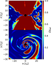 |
Fig. A.1. Meridional (top) and the equatorial (bottom) planes of the central region of the t = 23600 M, showing the normalized efficiency ( |

Appendix B: Fitting results
Figure B.1 shows the distribution of values for the ring flux and thickness resulting from fitting our models to both of our datasets, computed at the central value of GM/Dc2. The total flux of the ring is well behaved at 86 GHz and is biased toward lower values at 230 GHz, where the Gaussians carry part of the total flux of the image. Indeed, Event Horizon Telescope Collaboration (2019e) find that the additional Gaussian components in their model can account for anywhere between 10% and 70% of the total flux of the 2017 230 GHz data. Similarly, at 86 GHz the ring thickness is normally distributed with a mean value of 29.2 ± 1.8 μas, while the 230 GHz fittings are biased toward thin rings, with half of them returning ring thickness values of < 5 μas. We hypothesize this to be affected by the Gaussians partly modeling the thickness in the location of the hotspots, while a thinner ring takes care of the underlying structure.
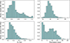 |
Fig. B.1. Normalized distribution of the flux and thickness resulting from fitting our models to the 86 GHz (top) and 230 GHz (bottom) datasets, complementary to Fig. 6. |
Figure B.2 shows the full posterior distribution with all seven parameters for a specific time step at 86 GHz. Using dynesty allows us to evaluate the convergence of the model. In this case, the diagonal 1D histograms show that the optimization converged without an issue, returning normal distributions for every parameter. The off-diagonal 2D histograms show correlations between parameters through deviations from a 2D normal distribution. For example, the diameter-thickness plot shows that the Bayesian optimization found an inverse relation between the thickness and the diameter at this time step.
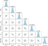 |
Fig. B.2. Bayesian posterior distributions of the thick m-ring model to the 86 GHz data at t = 26000 M. The diagonal panels show the posterior distributions and the most probable value of each parameter, given as the median value. The vertical dashed lines show this median value as well as the 2σ range, which is taken as the upper and lower error. The 2D histograms show the joint distributions of each parameter pair (row and column-wise) that shows possible correlations. Contours have been drawn following the samples at different intervals. The innermost shaded area contains samples with a likelihood of 0.5σ, and the outer contours contain the 1σ, 1.5σ, and 2σ likelihoods. The total extent of the plots corresponds to a 5σ likelihood. |
Appendix C: Symmetric models
We selected the 60 time steps between t = 24000 M and t = 30 000 M, with a cadence of tcad = 100 M, and computed the χ2 of fitting different models to their synthetic visibilities. Table C.1 shows the χ2 values of different models, averaged over all sixty time steps. We show the results of fitting to data with the observational errors of Lu et al. (2023), as well as with an additional fractional error of 10% to the visibilities observed by ALMA.
Time-averaged χ2 values for different morphologies and setups on 86 GHz data.
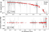 |
Fig. C.1. Visibility amplitude over uv distance for the time step t = 26700 M. Overlaid in red is the result of fitting a thick m-ring model to the data. Note the relatively few nonzero closure phases. |
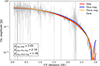 |
Fig. C.2. Visibility amplitudes over uv distance for the image at t = 26700 M. Plotted on top are the results of fitting three different azimuthally symmetric models to the data. The χamp2 values have been computed accounting for an additional 10% error on ALMA data. |
In addition to the asymmetric thick m-ring model, we also fit a top-hat disk, an infinitesimally thin ring, and a thick ring to our test data. Table C.1 shows that adding a 10% error on ALMA baselines reduces the χ2 values by an order of magnitude for the symmetric morphologies. While χ2 are expected to improve with increasing errors, as shown by Eqs. 19 and 20, it is noteworthy that the thick m-ring provides a better fit without additional errors than the symmetric morphologies do with these errors. However, examining the individual time steps shows a large range of χ2 values. Within our subset, t = 26700 M contains the data with the best χcp2 values for the symmetric models. With the added ALMA errors, the disk, thin ring and thick ring models obtain χcp2 values of 0.66, 0.85 and 0.66, respectively. Without the added ALMA errors it is instead χcp2 = 1.82, 6.69 and 1.82. The symmetric models also perform relatively well on the amplitudes, with χamp2 values of 2.05, 2.10 and 1.78 for the disk, thin ring and thick ring, respectively, when we include additional ALMA errors. Without them, we obtain χamp2 values of 6.73, 11.35 and 6.66, indicating a bad fit but better than the average of Table C.1. Figure C.1 shows the thick m-ring fitting for this time step. Compared to Fig. 5, it is clear that there are fewer nonzero closure phases, as expected of a time step where symmetric models would perform well. Indeed, Fig. C.2 shows the fit of all three of these models on top of the t = 26700 M amplitudes. The models largely retrieve the features of this time step.
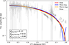 |
Fig. C.3. Visibility amplitudes over uv distance for the image at t = 28600 M. Plotted on top are the results of fitting three different azimuthally symmetric models to the data. The χamp2 values have been computed accounting for an additional 10% error on ALMA data. |
By comparison, Fig. C.3 contrasts the performance of the symmetric morphologies on the same time step as Fig. 5, where several asymmetric features are present. Even with ALMA errors, these models return χamp2 values of around 8 − 9. Without errors, the disk, thing ring and thick ring models respectively return χamp2 values of 189.04, 197.87 and 165.39. The χcp2 values are all around 26. The data at t = 26700 M have a clear lack of asymmetric features compared to the data at t = 28600 M. This asymmetry is visible not only in the nonzero closure phases, but also in structures present in the visibility amplitudes that cannot be fit by unmodulated Bessel functions.
Appendix D: 230 GHz model
We used the same test dataset at 230 GHz as the one used at 86 GHz in Appendix C. Applying the simple thick m-ring model to 230 GHz data yielded average χ2 values of χamp2 = 37.4 and χcp2 = 23.0. The inclusion of two free Gaussian components brings our fit to χamp2 = 1.71 and χcp2 = 1.85.
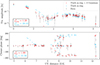 |
Fig. D.1. Visibility amplitudes and closure phases over uv distance for the time step t = 28900 M. Overlaid in blue is the result of fitting the same m = 2 thick m-ring that we previously fit to 86 GHz data. The model corresponding to the red data points, by contrast, contains two free Gaussian features. |
Figure D.1 compares the result of fitting an m = 2 thick m-ring model to the same time step with and without the free Gaussians. The extra Gaussian features are particularly necessary for modeling the visibility amplitudes between 1.2 and 1.5 Gλ, corresponding to the LMT-SMT (Submillimeter Telescope) baseline, as well as the closure phases between 6 and 7 Gλ, corresponding to the ALMA-SMT-LMT triangle.
Appendix E: Impact of the field of view
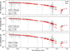 |
Fig. E.1. Visibility amplitudes over uv distance for the time step t = 24500 M. Overlaid in red is the thick m-ring model fit to each set of visibilities. Each panel corresponds to visibilities computed from the central image with different fields of view. |
Figure E.1 shows the results of fitting our m-ring model to the visibilities of a representative time step, computed from the central 100 μas, 140 μas and 1 mas. Increasing the FOV incorporates more of the bulk emission into the visibilities, resulting in higher amplitudes at the shortest baselines and more complex, less ring-like structures at the longest baselines. The fit to the longest baselines is critical to study the diameter of a ring model, as this quantity is related to the first nulls in the Bessel functions that comprise the Fourier transform of a ring. Similarly, the second nulls are related to the thickness of said ring. As this uv coverage does not contain long enough baselines to probe these second nulls, the curvature of the data after the first null at the longest baselines is all that the model has to estimate the thickness of the ring. We find that increasing the FOV not only worsens the quality of the fit, but it also increases the thickness while keeping the diameter roughly constant. On our test dataset, performing the fitting on data with FOV = 100 μas, 140 μas, and 1 mas resulted in median diameters of 53.1 μas, 53.2 μas, and 55.6 μas, respectively. On the other hand, the fits returned for the median values of the thickness 28.8 μas, 38.6 μas, and 46.3 μas. This shows a high sensitivity of the ring thickness on the selected FOV, which is expected due to the limited uv coverage at the necessary spatial frequencies. We decided on 100 μas based on the quality of the fits so as to prevent the bulk of the extended emission from dominating the fit.
All Tables
Antennas involved in the observations used to generate synthetic data and their nominal sensitivities.
All Figures
|
Fig. 1. Evolution of our GRMHD simulation over time. The top and middle panels show the logarithm of the density in the equatorial and a meridional plane, respectively, for three different times. The bottom panel shows the temporal evolution of the mass accretion rate (Ṁ) and the MAD parameter, |
| In the text | |
|
Fig. 2. Results of the GRRT calculations at t = 26 000 M. The images show the flux density at 86 GHz and 230 GHz. Notice that the images are convolved with half of the nominal resolution of the GMVA (27 μas) and the EHT (10 μas), indicated by the white circle at the bottom right. The contours begin at 1/1000 of the maximum flux density and increase by factors of two. In the bottom panel we display the broadband radio spectrum of our model. The observational flux values are taken from Prieto et al. (2016), Perlman et al. (2001), Whysong & Antonucci (2004), Hada et al. (2017), and Lister et al. (2018). |
| In the text | |
|
Fig. 3. Structural decomposition of the horizon scale structure in our model at t = 26 000 M. The panels show from left to right the total, disk, and jet plus wind contributions for 86 GHz (top row) and 230 GHz (bottom row). |
| In the text | |
|
Fig. 4. Fourier transforms of the central regions of our simulated data at t = 24 500 M. Plotted on top is the u − v coverage at 86 GHz and 230 GHz used for the generation of synthetic observations, using the array configurations presented in Lu et al. (2023) and Event Horizon Telescope Collaboration (2019a), respectively. Note the different scales in the two plots. |
| In the text | |
|
Fig. 5. Visibility amplitudes and closure phases over uv distance for the time step t = 28 600 M at 86 GHz. Overlaid in red is the result of fitting a thick m-ring model to the data. The χ2 values have been calculated taking an additional 10% error into account for ALMA visibilities. |
| In the text | |
|
Fig. 6. Normalized distribution of the diameters resulting from fitting our models to the 86 GHz and 230 GHz datasets. The other parameters can be found in Appendix B. The vertical lines show the central observational values (solid) as well as upper and lower range (dashed) of the ring diameter at both frequencies. We use the range found by Event Horizon Telescope Collaboration (2019a) at 230 GHz. At 86 GHz, we plot the range found by Lu et al. (2023) and the range found by Kim et al. (2025) using the resolve algorithm. |
| In the text | |
|
Fig. 7. Distribution of the diameters resulting from fitting our models to the 86 GHz and 230 GHz datasets. The turquoise and orange histograms show, respectively, the result of model fitting to GRRT data with an angular scale of 3.8 μas and 4.2 μas. The vertical lines show the observational range for the diameter of the ring, using the same values as Fig. 6. |
| In the text | |
|
Fig. 8. Normalized distribution of the absolute values and argument for the m = 1, 2 beta modes resulting from the model fitting of the 86 GHz data. |
| In the text | |
|
Fig. 9. Four time steps that display different ring morphologies (clockwise from the top left): dipole-dominant, quadrupole-dominant, complex, and ring-like. The more complex structure is caused by nonzero beta modes that are comparable in magnitude. |
| In the text | |
|
Fig. 10. Comparison of the underlying GRRT data and the output of our model fitting at 230 GHz (top) and 86 GHz (bottom) for t = 29 800 M. Right column: Output of the GRRT calculations, non-blurred. Central column: Same GRRT images, blurred by a beam of 10 μas and 27 μas for 230 GHz and 86 GHz, respectively. Left column: Parametrized model resulting from our fitting procedure, blurred with those same beams. All plots have been normalized to their maximum flux for ease of comparison. Note the increased surrounding flux at 86 GHz in the right column. |
| In the text | |
|
Fig. 11. Distribution of the turnover frequency, turnover flux density, and optically thin spectral index for a mixed eDF of thermal and kappa distribution (top) and thermal eDF only (bottom) at t = 24 000 M. |
| In the text | |
|
Fig. 12. Evolution of a MAD event in the equatorial plane. Top row: Logarithm of the density with overlaid contours indicating locations of particle acceleration, where |
| In the text | |
|
Fig. 13. Distribution of the diameters resulting from fitting our models to the 86 GHz and 230 GHz datasets. The data are the same as in Fig. 6, here shown split into the time steps before and after t = 24 000 M. The black outline shows the total distribution, corresponding to that of Fig. 6. The vertical lines show the observational range for the diameter of the ring, using the same values as Fig. 6. |
| In the text | |
|
Fig. A.1. Meridional (top) and the equatorial (bottom) planes of the central region of the t = 23600 M, showing the normalized efficiency ( |
| In the text | |
|
Fig. B.1. Normalized distribution of the flux and thickness resulting from fitting our models to the 86 GHz (top) and 230 GHz (bottom) datasets, complementary to Fig. 6. |
| In the text | |
|
Fig. B.2. Bayesian posterior distributions of the thick m-ring model to the 86 GHz data at t = 26000 M. The diagonal panels show the posterior distributions and the most probable value of each parameter, given as the median value. The vertical dashed lines show this median value as well as the 2σ range, which is taken as the upper and lower error. The 2D histograms show the joint distributions of each parameter pair (row and column-wise) that shows possible correlations. Contours have been drawn following the samples at different intervals. The innermost shaded area contains samples with a likelihood of 0.5σ, and the outer contours contain the 1σ, 1.5σ, and 2σ likelihoods. The total extent of the plots corresponds to a 5σ likelihood. |
| In the text | |
|
Fig. C.1. Visibility amplitude over uv distance for the time step t = 26700 M. Overlaid in red is the result of fitting a thick m-ring model to the data. Note the relatively few nonzero closure phases. |
| In the text | |
|
Fig. C.2. Visibility amplitudes over uv distance for the image at t = 26700 M. Plotted on top are the results of fitting three different azimuthally symmetric models to the data. The χamp2 values have been computed accounting for an additional 10% error on ALMA data. |
| In the text | |
|
Fig. C.3. Visibility amplitudes over uv distance for the image at t = 28600 M. Plotted on top are the results of fitting three different azimuthally symmetric models to the data. The χamp2 values have been computed accounting for an additional 10% error on ALMA data. |
| In the text | |
|
Fig. D.1. Visibility amplitudes and closure phases over uv distance for the time step t = 28900 M. Overlaid in blue is the result of fitting the same m = 2 thick m-ring that we previously fit to 86 GHz data. The model corresponding to the red data points, by contrast, contains two free Gaussian features. |
| In the text | |
|
Fig. E.1. Visibility amplitudes over uv distance for the time step t = 24500 M. Overlaid in red is the thick m-ring model fit to each set of visibilities. Each panel corresponds to visibilities computed from the central image with different fields of view. |
| In the text | |
Current usage metrics show cumulative count of Article Views (full-text article views including HTML views, PDF and ePub downloads, according to the available data) and Abstracts Views on Vision4Press platform.
Data correspond to usage on the plateform after 2015. The current usage metrics is available 48-96 hours after online publication and is updated daily on week days.
Initial download of the metrics may take a while.