| Issue |
A&A
Volume 705, January 2026
|
|
|---|---|---|
| Article Number | A20 | |
| Number of page(s) | 14 | |
| Section | Numerical methods and codes | |
| DOI | https://doi.org/10.1051/0004-6361/202556174 | |
| Published online | 23 December 2025 | |
Accurate N-body simulations with local primordial non-Gaussianities: Initial conditions and aliasing
1
Departamento de Física Teórica, Universidad Autónoma de Madrid,
28049
Madrid,
Spain
2
Centro de Investigación Avanzada en Física Fundamental (CIAFF), Facultad de Ciencias, Universidad Autónoma de Madrid,
28049
Madrid,
Spain
3
Instituto de Física Teorica UAM-CSIC,
c/ Nicolás Cabrera 13–15, Cantoblanco,
28049
Madrid,
Spain
4
Institut de Física d’Altes Energies (IFAE) The Barcelona Institute of Science and Technology campus UAB,
08193
Bellaterra Barcelona,
Spain
5
Centro de Investigaciones Energéticas, Medioambientales y Tecnológicas (CIEMAT),
Madrid,
Spain
6
Department of Astrophysics, University of Vienna,
Türkenschanzstrasse 17,
1180
Vienna,
Austria
7
Department of Mathematics, University of Vienna,
Oskar-Morgenstern-Platz 1,
1090
Vienna,
Austria
8
Serra Húnter Fellow, Departament de Física, Universitat Autónoma de Barcelona, Edifici C Facultat de Ciències,
08193
Bellaterra,
Spain
★ Corresponding author: This email address is being protected from spambots. You need JavaScript enabled to view it.
Received:
30
June
2025
Accepted:
8
October
2025
Abstract
The new generation of galaxy surveys designed to constrain local primordial non-Gaussianity (PNG) requires N-body simulations that accurately reproduce its effects. In this work, we explore various prescriptions for the initial conditions of simulations with PNG, seeking to optimise accuracy and minimise numerical errors, particularly due to aliasing. We used 186 runs that vary the starting redshift, Lagrangian Perturbation Theory (LPT) order, and non-Gaussianities (fNLlocal and gNLlocal). Starting with third order LPT (3LPT) at a redshift as low as zstart ≃ 11.5 reproduces to <1% the power spectrum, bispectrum, and halo mass function of a high-resolution reference simulation. The aliasing induced by the PNG terms in the power spectrum produces a ≤3% excess for small-scales at the initial conditions. This excess drops below 0.1% by z = 0. State-of-the-art initial condition generators show a sub-percent agreement. We show that initial conditions for simulations with PNG should be established at a lower redshift using higher-order LPT schemes. We also show that removing the PNG aliasing signal is unnecessary for current simulations. The methodology proposed here can accelerate the generation of simulations with PNG while enhancing their accuracy.
Key words: methods: numerical / large-scale structure of Universe
© The Authors 2025
 Open Access article, published by EDP Sciences, under the terms of the Creative Commons Attribution License (https://creativecommons.org/licenses/by/4.0), which permits unrestricted use, distribution, and reproduction in any medium, provided the original work is properly cited.
This article is published in open access under the Subscribe to Open model. This email address is being protected from spambots. You need JavaScript enabled to view it. to support open access publication.
1 Introduction
Numerical simulations are a powerful tool for cosmology, as they can accurately model structure formation deep into the non-linear regime (k > 1 h Mpc−1), where perturbative analytical methods break down. Today, simulations are fundamental at nearly every phase of large-scale structure (LSS) analysis. They play a key role in developing data processing pipelines for extracting the cosmological information (e.g. Noriega et al. 2025; Krause et al. 2017; Alam et al. 2021; Riquelme et al. 2023), estimating the covariance matrices (Avila et al. 2018; Zhao et al. 2021; Ereza et al. 2024; Forero-Sánchez et al. 2025), and evaluating the impact of observational systematics (Ross et al. 2017; Bianchi et al. 2018; Chan et al. 2022; Chaussidon et al. 2025).
Until recently, the statistical power of galaxy surveys was the main bottleneck for cosmological inference (LSST Science Collaboration 2009; Weinberg et al. 2013). However, the current limiting factor is shifting towards theoretical and numerical modelling, as seen in experiments such as the Dark Energy Spectroscopic Instrument (DESI) (DESI Collaboration 2016) and Euclid (Laureijs et al. 2011), as well as in forthcoming facilities such as the Rubin Observatory (LSST Science Collaboration 2009). Improving analytic models demands parallel advances in simulation accuracy, where a good understanding of the parameters that control numerical precision is required (Power et al. 2003; Heitmann et al. 2010; Schneider et al. 2016).
Primordial non-Gaussianity (PNG) is a key target of upcoming surveys, offering a direct window into inflationary physics. The simplest single-field slow-roll models for inflation predict that curvature perturbations are nearly Gaussian (Baumann 2012; Riotto 2017). This implies that all the statistical information is contained in the two-point correlation function or its Fourier equivalent, the power spectrum. One way to look for departures from Gaussianity is to study the three-point function (bispectrum). In standard single-field scenarios, the bispectrum amplitude, fNL, in the squeezed limit (k1 ∼ k2 ≫ k3) is (ns − 1) (Maldacena 2003; Creminelli & Zaldarriaga 2004). Thus, detecting | fNL| ≳ 1 would be enough to rule out canonical single-field slow-roll inflation. At the same time, a measured value of fNL ∼ (ns − 1) would severely constrain other inflationary models (Bartolo et al. 2004; Byrnes et al. 2010).
Models that propose that inflation is driven by multiple fields can naturally lead to | fNL| ∼ 1 (Byrnes & Choi 2010; Chen 2010). An example of these models is the curvaton inflation (e.g. Lyth & Wands 2002; Lyth et al. 2003). Such scenarios can be parametrised in terms of the local PNG as
 (1)
where ϕG is the Gaussian primordial gravitational potential and
(1)
where ϕG is the Gaussian primordial gravitational potential and  controls the non-Gaussian quadratic correction (Komatsu & Spergel 2001; Salopek & Bond 1990).
Currently, the strongest bounds on local-type PNG come from measurements of the bispectrum of temperature fluctuations of the cosmic microwave background (CMB), leading to fNL = −0.9 ± 5.1 (68% c.1.) (Planck Collaboration IX 2018). However, the amount of information that we can extract from the CMB about local PNG is limited by cosmic variance. For this reason, it is not expected to go beyond σ( fNL) ∼ 3 with CMB-only data (Komatsu & Spergel 2001; Babich & Zaldarriaga 2004). An alternative method has been proposed to beat these constraints by analysing the LSS of the Universe. The core idea is to use the scale-dependent bias (b2 = Pgg(k)/Pmm(k) ∝ 1/k4 at large scales) that local PNG induces in galaxy clustering (Dalal et al. 2008; Slosar et al. 2008; Matarrese & Verde 2008).
The most stringent constraints from the LSS method come from the first year of data of the DESI survey, where they found  (68% c.1.) (Chaussidon et al. 2025). Forecasts for Stage IV surveys including information from the bispec-trum (Tellarini et al. 2016; Karagiannis et al. 2018), multi-tracer techniques (Barreira & Krause 2023; Sullivan et al. 2023; Karagiannis et al. 2024), and data from upcoming experiments such as SphereX (Doré et al. 2015; Shiveshwarkar et al. 2024) are expected to reach σ(fNL) ∼ 0.5 (Ballardini et al. 2019; Heinrich et al. 2024).
To distinguish between the more canonical inflationary models and other scenarios, new surveys have been designed with increasingly smaller target σ(fNL), for example SphereX (Doré et al. 2015) and SPEC-S5 (Besuner et al. 2025). As a result, simulations that accurately include PNG are growing in importance. Significant efforts have been made to produce realistic simulations for these surveys (e.g. Adame et al. 2024; Hadzhiyska et al. 2024; Bayer et al. 2025). A key challenge in running simulations in general, and PNG simulations in particular, is ensuring they are accurate enough. In the past, the community carried out large code comparison projects by running the same initial conditions with different N-body codes, leading to a 1% agreement among them in the matter power spectrum at k = 10 h Mpc−1 (e.g. Schneider et al. 2016; Garrison et al. 2019; Springel et al. 2021).
Building on these convergence benchmarks, attention has now shifted to mitigating the numerical artefacts that remain a threat to sub-percent accuracy in forthcoming PNG simulations. Discreteness effects from the particle lattice self-interactions have been a prominent concern (Joyce et al. 2005; Joyce & Marcos 2007; Garrison et al. 2016). Several proposals have been made to overcome these issues with tessellation methods (Hahn et al. 2013; Hahn & Angulo 2016; Sousbie & Colombi 2016; Stücker et al. 2020). N-body codes can be affected by significant numerical errors when computing forces against nearly uniform density fields at a high redshift. This motivates the idea of pushing the initial redshift to lower redshifts, where these effects are suppressed (Schneider et al. 2016; Michaux et al. 2020; Stahl et al. 2024a).
In this work we pursue three goals: (i) validating how the initial redshift and LPT order affect convergence in the presence of local PNG, (ii) quantifying PNG aliasing effects, and (iii) testing consistency among state-of-the-art codes for IC generation. The PNG initial condition generation step adds its own subtleties. The computation of the fields ϕ2 and ϕ3 on a discrete grid excite modes that cannot be represented in the original grid and fold back. This contaminates higher-frequency modes and induces a spurious signal. This effect is known as aliasing. The aliasing of the power spectrum and bispectrum estimation, and the computation of higher-order corrections in the LPT expansion has been well studied in the past (e.g. Sefusatti et al. 2016; Michaux et al. 2020). However, the majority of previous studies using PNG simulations have ignored the aliasing due to PNG altogether. Although some studies have accounted for (and corrected for) the aliasing (e.g. Stahl et al. 2023; Stahl et al. 2023, 2024b, 2025), to our knowledge its impact has not been explicitly quantified before. We also compared different state-of-the-art codes for generating the initial conditions for PNG simulations, namely MONOFONIC (Michaux et al. 2020; Hahn et al. 2020), 2LPTPNG (Crocce et al. 2006; Scoccimarro et al. 2012), FASTPM (Feng et al. 2016), and LPICOLA (Howlett et al. 2015).
This paper is structured as follows. In Section 2, we introduce how initial conditions are generated for cosmological simulations. We also discuss how this is done for PNG simulations, particularly how aliasing arises in these cases, and how it can be corrected. We then describe in Section 3 the simulation suite that we have produced to demonstrate all these points. We present our results in Section 4. We first discuss the impact of the initial redshift and LPT order. Then, we demonstrate the impact of aliasing, and compare some of the state-of-the-art codes for initial condition generation. Finally, we summarise our results and draw our conclusions in Section 5.
2 Methods
Cosmological N-body simulations are essential for tracking the growth of structures deep into the non-linear regime, where perturbative techniques fail. State-of-the-art codes such as PKD-GRAV3 (Potter et al. 2017) and GADGET4 (Springel et al. 2021) integrate the equations of motion for a large number of phase-space tracers (particles), capturing the evolution from the smooth early density field to the web of filaments, sheets, and virialised halos observed today.
To generate the initial conditions (ICs) for these simulations, we must specify the positions and velocities of every particle at a given point in the past. The accuracy of these ICs determines the upper limit on the precision for any late-time statistic that can be modelled with the simulation. Typically, a random realisation of the density field matching the linear power spectrum is generated, which then is back scaled to the desired initial redshift. Then the displacements and velocities of the particles are obtained using the Lagrangian perturbation theory truncated at some low order. In what follows, we describe these standard algorithms used to build Gaussian ICs and then show how they can be extended to include local-type primordial non-Gaussianity.
2.1 Generating initial conditions for N-body simulations
The most popular method to initialise cosmological N-body simulations is the back-scaling method (see Sect. 6 from Angulo & Hahn 2022, for a review). The first step is to solve the coupled Einstein–Boltzmann equations using, for example, CAMB (Lewis et al. 2000) or CLASS (Lesgourgues 2011). These codes evolve all relevant species (cold dark matter, baryons, photons, massive neutrinos, . . . ) down to the target redshift for the final desired output of the simulation, ztarget. The resulting linear total-matter density contrast δm(k, ztarget) is then rescaled to the initial redshift zstart at which the N-body run begins,
 (2)
where D+(z) is the linear growth factor normalised to D+(0) = 1. By construction, the back-scaled field reproduces the exact linear solution at ztarget, including scale-dependent effects of radiation and massive neutrinos, while neglecting the decaying modes. These modes are already strongly suppressed by zstart if starting late enough. Although this procedure yields a fictitious radiation content at the initial time, it remains fully consistent with relativistic perturbation theory when the system is evolved forward with Newtonian dynamics (Chisari & Zaldarriaga 2011; Hahn & Paranjape 2016; Fidler et al. 2017).
(2)
where D+(z) is the linear growth factor normalised to D+(0) = 1. By construction, the back-scaled field reproduces the exact linear solution at ztarget, including scale-dependent effects of radiation and massive neutrinos, while neglecting the decaying modes. These modes are already strongly suppressed by zstart if starting late enough. Although this procedure yields a fictitious radiation content at the initial time, it remains fully consistent with relativistic perturbation theory when the system is evolved forward with Newtonian dynamics (Chisari & Zaldarriaga 2011; Hahn & Paranjape 2016; Fidler et al. 2017).
To generate the initial conditions, we have to specify a particular realisation of the density field δm. This is modelled as a Gaussian random field (if there are no PNGs) whose variance is given by the power spectrum. We begin with a complex random white noise field, W(k), given by
 (3)
where both, real and imaginary parts are sampled from a Gaussian distribution with zero mean and unit variance. The power spectrum in the density field is induced via
(3)
where both, real and imaginary parts are sampled from a Gaussian distribution with zero mean and unit variance. The power spectrum in the density field is induced via
 (4)
where Plin(k, zstart) is the desired linear matter power spectrum obtained from the Boltzmann solver. Then, to make sure that δm(x) is real, we impose
(4)
where Plin(k, zstart) is the desired linear matter power spectrum obtained from the Boltzmann solver. Then, to make sure that δm(x) is real, we impose  .
.
When we work with PNGs, it is often more convenient to operate with the primordial gravitational potential ϕ instead of the matter density contrast δm. These two quantities can be used interchangeably as they are related via the Poisson equation. In Fourier space, this interchangeability can be expressed as
 (5)
where α(k) is defined as
(5)
where α(k) is defined as
 (6)
(6)
Here H0 is the Hubble parameter, Ωm,0 is the matter density at z = 0 and c is the speed of light. T(k) is the matter transfer function normalised to T(k → 0) = 1, D+ is the growth factor normalised to D(z = 0) = 1, and g(z) = (1 + z)D+(z). The term  arises precisely because of the choice of this normalisation for the growth factor. We evaluate g(z) at radiation domination, so for the cosmology chosen here (see Table 2), the value of
  is ∼1.2741.
With these definitions, the linear matter power spectrum can be written compactly as
 (7)
where Pϕ(k) is the power spectrum of the primordial gravitational potential. This is set during inflation via
(7)
where Pϕ(k) is the power spectrum of the primordial gravitational potential. This is set during inflation via
 (8)
with k∗ the pivot scale and As the amplitude of the primordial fluctuations, such that
(8)
with k∗ the pivot scale and As the amplitude of the primordial fluctuations, such that  .
.
The stochasticity of the white noise is what leads to the cosmic variance in the simulations. One can take advantage of how this noise is generated to suppress much of this variance. For example, generating two realisations where phases are shifted by a factor of π with respect to each other leads to inverted realisations (i.e. high-density peaks in one simulation become voids and vice versa) (Pontzen et al. 2016). This is precisely what we do in this paper to improve the measurements of the summary statistics.
Another option is to remove all the stochasticity in the amplitude part of the white noise, leading to a realisation with suppressed variance. Combined with the previous one, this idea composes the fixed-and-paired method (Angulo & Pontzen 2016). Moreover, keeping the same white noise seed across simulations with different cosmologies (e.g. fNL = 0 vs fNL ≠ 0) leads to correlations that can be used to improve the measurements of cosmological parameters via the difference between simulations (Avila & Adame 2022; Adame et al. 2024).
Once the realisation of the initial overdensity field (or primordial potential) is generated, the next step is to obtain the initial displacements and velocities for the particles. For that, the particles are first placed on an unperturbed cubic lattice, q, representing the homogeneous Universe at a → 0. Their Eulerian positions at zstart follow from Lagrangian perturbation theory (LPT),
 (9)
(9)
Here, Ψ(1) corresponds to the Zeldovich approximation (Zel’dovich 1970) and captures the leading-order displacements. The second-order term, Ψ(2), introduces non-linear, curl-free corrections, while Ψ(3) includes higher-order contributions, capturing vorticity modes that are absent at lower orders (e.g. Bouchet et al. 1995; Rampf 2012). The peculiar velocity of the particles is given by  . For a detailed derivation of these displacement fields, we refer to Zel’dovich (1970); Bouchet et al. (1992, 1995); Rampf (2012).
The codes used to generate initial conditions, such as those presented in Section 3.2, compute these displacement fields from the overdensity field. They then output particle positions and velocities in a format adequate to run a N-body code.
2.2 Primordial non-Gaussianity
While single-field slow-roll inflation predicts a nearly Gaussian primordial spectrum of perturbations, with departures of the order (ns − 1) (Maldacena 2003; Creminelli & Zaldarriaga 2004), non-standard inflationary scenarios can produce observable non-Gaussianities (Chen 2010; Byrnes & Choi 2010).
Primordial non-Gaussianities (PNGs) are most commonly studied through their imprint on the three-point function (or bis-pectrum) of the IC or primordial field. In this work, we focus on the local type of PNG, in which the non-Gaussian potential is usually parametrised as (Salopek & Bond 1990; Komatsu & Spergel 2001):
 (10)
where ϕG is the Gaussian potential while the amplitudes fNL and gNL control the quadratic and cubic deviations respectively.
(10)
where ϕG is the Gaussian potential while the amplitudes fNL and gNL control the quadratic and cubic deviations respectively.
Current constraints from the Planck temperature and polarisation data are  (68% c.1.),
  (68% c.1.) (Planck Collaboration IX 2018), close to the cosmic variance limit. Future improvements must come from large-scale structure surveys, which can potentially reach sensitivities of | fNL| ∼ 1 (Ballardini et al. 2019; Heinrich et al. 2024), enough to rule out single-field slow-roll models (which predict | fNL| ≪ 1).
A powerful probe of local PNG in the galaxy or halo clustering is the emergence of a scale-dependent bias on large scales. In the presence of local PNG, the linear bias expansion of the halo overdensity field, δh, acquires an extra term proportional to the primordial potential:
 (11)
(11)
Here b1 is the linear bias and bϕ is the bias parameter associated with the fNLϕ operator. Physically, bϕ represents how halos respond to the presence of local PNG. Using the Poisson equation (Equation (5)), one substitutes ϕ by δm, which yields:
 (12)
which exhibits an enhancement proportional to k−4 on the largest scales. Consequently, larger survey volumes dramatically improve the sensitivity to measure fNL.
(12)
which exhibits an enhancement proportional to k−4 on the largest scales. Consequently, larger survey volumes dramatically improve the sensitivity to measure fNL.
A key challenge is the degeneracy between fNL and the bias parameter bϕ, quantifying how the tracer responds to large-scale potential fluctuations. Under the assumption of a universal halo mass function, that is, depending only on mass, the universality relation is predicted (Dalal et al. 2008; Matarrese & Verde 2008):
 (13)
(13)
Here δc ≃ 1.686 the spherical collapse threshold. However, numerical and analytic studies reveal deviations from this relation for specific halo samples (e.g. Slosar et al. 2008; Grossi et al. 2009; Hamaus et al. 2011; Lazeyras et al. 2023; Adame et al. 2024) and for galaxies (e.g. Barreira et al. 2020; Voivodic & Barreira 2021; Marinucci et al. 2023). To capture the deviations from the universality relation, the following parametrisation is commonly used,
 (14)
where the PNG-response parameter p is measured from simulations and can depend on the tracer sample.
(14)
where the PNG-response parameter p is measured from simulations and can depend on the tracer sample.
2.3 Initial conditions for local-PNG simulations
To generate initial conditions with local PNG, Equation (10) is applied to the Gaussian potential before computing the LPT displacements. Alternative methods have been discussed in the literature. Convolving ϕ with a given kernel allows the generation of non-Gaussianities with an arbitrary bispectrum (Wagner & Verde 2012; Scoccimarro et al. 2012). The local PNG case can be recovered for a specific choice of kernel.
We note that local non-Gaussianities not only couple the long-wavelength perturbations with the short-wavelength ones but also change the depth of the gravitational potential wells. This can alter the collapse of structures, potentially varying the regime of validity of the LPT approximation and hence the conclusions from Michaux et al. (2020) about pushing the initial redshift to lower values. Although LPT ceases to be formally valid after shell-crossing, their results indicated that one can still push to lower zstart if most of the volume remains in the perturbative regime. For example, in a simulation with a box size Lbox = 1 h−1 Gpc and Npart = 10243, the best agreement with the continuous limit occurs at zstart = 11.5 with 3LPT, for the configurations they tested. Although the role of the initial redshift and resolution was already explored in Stahl et al. (2024a) for scale-dependent fNL models, here we extend their analysis to pure local PNG models and we study higher-order and halo statistics, as well as how the LPT order may impact convergence.
Numerical aliasing arises because we represent continuous fields on a finite, discrete grid and must be accounted for to capture the modified potentials on a mesh accurately. The maximum frequency that can be represented on the grid, is the Nyquist wave number, defined as  , where N is the grid size, and kf is the fundamental mode,
  . Real-space operations (Equation (10)) like
  (and
(and  ) correspond to convolutions in Fourier space which inject power up to 2 kNyq (or 3 kNyq for the cubic term). Any mode beyond kNyq cannot be represented on the grid and is assigned (aliased) into lower-k modes, that is, those with k ≤ kNyq that the grid can represent. Because
  only reaches 2kNyq, while
  extends to 3 kNyq, the specific intervals of contaminated (aliased) modes differ, and hence the mitigation strategy.
Summary of the simulations ran with Npart = 5123 and Lbox = 1 h−1 Gpc, used to study the effect of LPT order, initial redshift, and aliasing in the presence of local PNG.
3 Simulations
We ran a suite of N-body simulations to study the generation of initial conditions for local PNG simulations and strategies to remove the PNG aliasing signal (dealiasing). The simulation suite consists of a set of 140 low-resolution simulations, Npart = 5123 and Lbox = 1 h−1 Gpc, with varying initial conditions. We used the LPT with orders from 1 to 3 and initial redshifts zstart = 99, 49, 24, 11.5. The LPT–zstart combinations we considered are listed in Table 1. We excluded combinations that previous works showed that do not improve accuracy. For example, previous studies showed that 1LPT fails well before zstart = 49, and that 2LPT can match the 3LPT performance at high redshift, rendering 3LPT unnecessary at zstart = 99. All the simulations presented in this paper assume the Planck cosmology summarised in Table 2 (Planck Collaboration VI 2020).
Regarding the local PNG models, we considered fNL = 0, ±100 and gNL = 0, ±107. As the simulation boxes are relatively small, lower | fNL| values would weaken the PNG signal, making it harder to study. The local non-Gaussianity of type gNL is expected to produce a stronger aliasing effect than fNL cosmologies. Given that ϕ ∼ 10−5 in the initial snapshot and that fNLϕ2 ∼ gNLϕ3 ∼ 10−8, a value of gNL = ±107 produces a fractional correction in ϕNG of the same order as fNL = ±100.
For every combination of initial redshift, zstart, and LPT order, we ran simulations at each amplitude of local PNG (fNL and gNL). Each configuration was executed in aliased and dealiased modes (see Section 3.1 for details). Every run also has two realisations with inverted phases, following Pontzen et al. (2016). To isolate systematic differences, we used MONOFONIC (Hahn et al. 2020; Michaux et al. 2020) to set all the initial conditions, and we fixed the same seed of white noise for all runs.
All the simulations presented here were evolved with the N-body code PKDGRAV3 (Potter et al. 2017; Alonso Asensio et al. 2023). This code uses the fast multipole method to compute the gravitational force. The algorithm implemented in the code provides a scaling (N) and takes advantage of GPUs for additional speed while maintaining high accuracy (see Garrison et al. 2019, for a comparison). We saved snapshots only at z = zstart and z = 0, at which we performed our study. Halos within the simulations were identified with Rockstar (Behroozi et al. 2012). This method is based on a friends-of-friends algorithm in the 6D phase space, using the positions and velocities of the particles. Only halos containing at least 20 particles were considered for our analysis.
Cosmological and input parameters of all simulations.
3.1 Removing the PNG aliasing signal
To assess the impact of the PNG aliasing signal, introduced in Section 2.3, we ran two pairs of simulations for each combination of zstart, LPT order, and fNL/gNL value (see Table 1). We refer to each pair as aliased and dealised. For the aliased simulations, we computed directly the ϕ2 term in the grid (i.e. naïve convolution), while for the de-aliased simulations, we used the Orszag 3/2 rule.
The Orszag 3/2 rule (Orszag 1971) has been previously used in the literature but not, to our knowledge, in the context of simulations with PNG. This method consists of: (i) padding the original Fourier grid with N3 cells with zeros up to (3/2 N)3; (ii) computing the non-linear product ϕ2 at this higher-resolution; (iii) truncating the grid back to the original size of N3. The zero padding by a factor of 3/2 in each dimension increases the memory footprint by (3/2)3 ≈ 3.4, which is often prohibitive if the original grid is already large. More generally, computing  without aliasing requires padding to ((n − 1)/2)N in each dimension (Patterson & Orszag 1971).
This Orszag 3/2 rule was already implemented within MonofonIC for computing the fields required for 2LPT and 3LPT (Michaux et al. 2020). In Stahl et al. (2023), this technique was extended also for removing the PNG aliasing. Here, we introduce the possibility of disabling the Orszag 3/2 convolver for the PNG part (while preserving it for the LPT part) for generating our dealised simulations.
For the cubic term, gNL, we avoid the direct 2N zero padding by performing two sequential convolutions. Using the 3/2 N padding, we first calculate  and then
  . Therefore, the maximum memory increase per pass is a factor (3/2)3 ∼ 3.4. This is well below the 23 = 8 of a one-shot cubic convolution, yet still free of aliasing.
Overview of the initial-condition generation codes used in this work.
3.2 Initial condition codes
To validate the robustness and accuracy of the primordial non-Gaussian implementation, we performed a controlled comparison of four state-of-the-art initial conditions (IC) generators: MonofonIC1 (Hahn et al. 2020; Michaux et al. 2020), 2LPTPNG2 (Scoccimarro et al. 2012), FastPM3 (Feng et al. 2016), and LPICOLA4 (Howlett et al. 2015). The last two codes are not dedicated IC generators but can act as such when instructed to write the initial snapshot. The LPT orders and PNG models available for each of the codes are summarised in Table 3.
MonofonIC implements local PNG through a convolution in real space, which is corrected for aliasing with the Orszag 3/2 technique (Section 3.1). In contrast, the public version of 2LPTPNG does not remove aliasing and resembles the naïve convolution in MonofonIC (Section 3.1). FastPM also uses real-space convolution but applies a low-pass filter to remove small-scale contributions. The parameter kmax_primordial_over_knyquist (kmax hereafter) controls at which scale this filter is applied. Finally, LPICOLA implements a different approach based on Scoccimarro et al. (2012) that allows the generation of general PNG (if it is compiled with the GENERIC_FNL flag). It can reproduce local PNG by choosing an appropriate kernel. The code also has the option to operate in the same way as 2LPTPNG (compiling with the LOCAL_FNL flag), but this is redundant for our comparison here.
We compared the four IC generators using identical settings to isolate how each code models the PNG signal. We generated 2LPT IC at zstart = 49 with fNL = 0, ±100. These are the common settings available to all codes, as shown in Table 3. We performed a total of 36 simulations for this study, with Npart = 10243 particles and the same box size as for all the simulations presented in this work, Lbox = 1 h−1 Gpc. We used a grid with the same N = 10243 to compute the LPT fields for the ICs and fix this choice consistently for all codes. We also tested increasing this number to 20483 and found that our results remain unchanged.
For FASTPM we varied the value of the parameter kmax, setting  and 1. FastPM applies a low-pass filter for the ϕ2 field at k = kmax · kNyq. This filter removes the PNG signal beyond the frequency kmax · kNyq, as shown in Figure 6. This is discussed in Section 4.3.
After running the simulations, we found that the white noise LPICOLA produces in the Gaussian mode (GAUSSIAN) is different from the one it generates when running the code in the general PNG mode (GENERIC_FNL) or the local PNG mode (LOCAL_FNL). The other three codes considered here generate a white noise compatible with the Gaussian LPICOLA. This results in larger relative differences in all statistics measured for LPICOLA compared to the other codes. Nevertheless, as we show below, all the differences are compatible with the cosmic-variance limit.
Parameters used to set up the initial conditions for the reference simulations for the three studies presented in this work.
3.3 Reference simulations
To study the impact of the parameter variations introduced above, we require a baseline set of runs that we refer to as the reference simulations. The reference simulations were run in a box side with side Lbox = 1 h−1 Gpc and Npart = 10243, providing a mass resolution eight times higher than for those runs with Npart = 5123. We ran Gaussian reference simulations, as well as with PNG, for fNL = ±100 and gNL = ±107. The ICs for all reference simulations were generated with MonofonIC and their main characteristics are summarised in Table 4. The PNG aliasing signal was removed with the Orszag 3/2 rule (see Section 3.1) for all the reference simulations.
For the analysis of the initial redshift, LPT order, and aliasing in the presence of local PNG (Sections 4.1 and 4.2), we generated the initial conditions at zstart = 24 using 3LPT. This choice, motivated by Michaux et al. (2020), balances accuracy with the risk of starting too late.
For the comparison of IC generators (Section 4.3), our reference simulations have IC generated with MonofonIC assuming 2LPT and zstart = 49. As the other codes cannot produce 3LPT initial conditions, our IC set-up is common to all the codes under study. This allows us to analyse the difference in the PNG implementation between the codes. We chose MonofonIC as our reference code because we have tested its convergence in Sections 4.1 and 4.2. Moreover, MonofonIC is the only code that supports dealiasing via the 3/2 zero-padding (see Section 3.1) among those considered here.
3.4 Measuring the power spectrum and bispectrum
We computed the power spectra with the Pylians package5 (Villaescusa-Navarro 2018). We assigned dark-matter particles onto a 10243 Cartesian density grid using a piecewise cubic spline (PCS) mass assignment scheme. Then, we measured the Fourier-space density contrast on that grid. With PCS, the aliasing correction is well understood, and the resulting estimate remains accurate up to the Nyquist wave number, kNyq :
 (15)
(15)
The same density grid was used for the bispectrum analysis. We used the GPU-accelerated code BFast6 to evaluate all triangle configurations in bins of width ∆k = 3kf up to  to avoid aliasing associated with the bispectrum estimator itself (Sefusatti et al. 2016). In our analyses, we focused on the squeezed limit of the bispectrum (k1 ~ k2 >>> k3), as this is the configuration in which most of the local PNG signal resides.
4 Results
In this section, we present how the variation of initial redshift, LPT order, and local PNG aliasing influences the accuracy of N -body simulations. We focus on the convergence of the matter power spectra, bispectra, and halo statistics. Our goal is to identify which simulation set-up and IC generation approach yields the most accurate results in the presence of local PNG for a given computational cost.
4.1 Initial redshift and LPT order
Michaux et al. (2020) demonstrated that starting N-body simulations at a lower redshift (i.e. a later start) and using higher-order LPT schemes improve their convergence towards the continuous limit.
We checked whether these findings also hold for local PNG. Positive fNL or gNL skews the one-point density distribution, enhancing the abundance of high-density regions, potentially causing earlier shell-crossing and narrowing LPT’s valid range. Conversely, negative fNL or gNL suppresses the high-density tails, delaying collapse and allowing a lower zstart. To investigate this, we performed simulations that varied the LPT order, initial redshift, and PNG parameters, as summarised in Table 1.
Varying the initial redshift and the order of the LPT schemes can affect the power spectrum and the bispectrum, as shown in Figure 1, where for the bispectrum, we show the squeezed limit (k1 = k2 = k, k3 = 3kf). The characteristics of the simulation used as a reference are discussed in Section 3.3. All power spectra and bispectra are shown in relation to that reference unless otherwise noted.
4.1.1 Power spectrum and bispectrum
For the power spectrum in the Gaussian case (fNL = 0), all starting redshift and LPT configurations agree at large scales (k < 0.1 h Mpc−1) but show a power suppression at smaller scales. This attenuation is stronger for higher zstart, up to a 5% at k = 1 h Mpc−1. Higher-order LPT realisations (e.g. 2LPT and 3LPT) at zstart = 49 converge to the same solution but are biased low compared to the reference. Because both cases show the same small-scale deficit relative to the reference, the effect cannot be traced to truncated perturbation theory but instead points to a discreteness-driven origin ( Michaux et al. 2020; Joyce et al. 2005).
A similar pattern emerged for the squeezed-limit bispectrum (lower panels of Figure 1), although it was more sensitive to the LPT order. The runs with 1 LPT remain systematically biased, while switching to higher-order LPT improves the agreement, as expected (McCullagh et al. 2016; Baldauf et al. 2015). We have focused on the squeezed limit as is the configuration that local PNG induces (e.g. Bartolo et al. 2004), although the equilateral configuration (k1 = k2 = k3 = k) showed 1–2% larger deviations. These findings were consistent with Michaux et al. (2020) in the Gaussian case.
We then performed the same analysis for fNL = ±100 and gNL = ±107 to check whether the local PNG changes this picture. The right panel in Figure 1 shows the fNL = 100 result. As in the Gaussian case, the convergence improved when starting the simulations at lower redshifts and employing higher-order LPT. Similar behaviour appeared for all other PNG parameters we tested, indicating that the results from Michaux et al. (2020) still hold for moderate to high fNL or gNL.
We note that all our conclusions are based on runs with |fNL| = 100 and |gNL| = 107. We expect that these conclusions also hold for smaller non-Gaussian amplitudes as they approach the Gaussian case, where this is also valid. However, larger fNL/gNL values may require more testing.
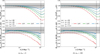 |
Fig. 1 Comparison at z = 0 of the matter power spectrum (upper panels) and bispectrum (lower panels, squeezed limit (k1 = k2 = k; k3 = 3kf)) with respect a high-resolution reference simulation (see Section 3.3). The left panel shows the results for fNL = 0 simulations, and the right panel for those with fNL = 100. The line colour encodes the LPT order used for the initial conditions (red: 1LPT, green: 2LPT, and blue: 3LPT), while the line styles indicate the initial redshift. The shaded regions indicate the ±1% around the reference simulation. The results are nearly identical for fNL = 0 and fNL = 100. A later start using higher-order LPT schemes improves the agreement with the higher-resolution reference simulations. |
4.1.2 Halo mass function
Next, we examine the impact on halo populations. We computed the halo mass function (HMF) in the bins ∆ log M = 0.1, shown in Figure 2. All runs showed a lack of low-mass halos at the level 10% – 20% for Mpart < 3 × 10¹³h−1M⨀. This is expected since the halos containing fewer than ~100 particles are not fully resolved (Power et al. 2003; Mansfield & Avestruz 2021). However, the deficit was less severe at later starts, regardless of the LPT order. In contrast, very early starts (e.g. zstart = 99) introduced a systematic ~4% bias across the entire mass range. Likewise, 3LPT at zstart = 11.5 best matched the reference of high resolution. Our local PNG runs (fNL = ±100, gNL = ±107) revealed the same picture, confirming that these recommendations are robust to moderate values of fNL or gNL.
These results reflect two competing effects. First, higher- order LPT schemes (e.g. 3LPT) provide more accurate displacements by including additional perturbative corrections, which formally improve convergence towards the fluid limit before shell-crossing. This is expected from theory, as the LPT expansion converges in powers of the linear growth factor D(z). However, at very early times (e.g. zini = 49), D(z) is small, so even low-order LPT (such as 2LPT) closely approximates the full solution, explaining why 2LPT and 3LPT are nearly indistinguishable in that regime. Second, discreteness effects due to the initial particle lattice become more prominent when starting too early (Michaux et al. 2020). These can be suppressed by initialising at lower redshifts, where the particle distribution has evolved away from the initial grid symmetry, and hence motivating the use of higher-order LPT schemes.
Lagrangian perturbation theory is only valid before shellcrossing. After this point, higher-order terms can actually diverge more rapidly from the true solution. Despite this limitation, our results show that even at very low starting redshifts (e.g. zstart = 11.5), 3LPT yields better agreement with high-resolution simulations than any of the earlier-start configurations we tested. These results might change for simulations with a different mass resolution.
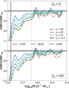 |
Fig. 2 Comparison at z = 0 of the halo mass function for different configurations of the initial conditions (see Section 3) with respect to the higher-resolution reference simulations (see Section 3.3). The upper panel shows the results for the fNL = 0 simulations, while the lower panel shows the case with fNL = 100. The line colour encodes the LPT order used for the initial conditions (red: 1LPT, green: 2LPT, and blue: 3LPT), while the line styles indicate the initial redshift. The dashed vertical lines show the limit of 20 particles per halo; the limit of 100 is indicated by the dash-dotted vertical lines. The shaded regions indicate the 1% difference around the reference simulation. Starting the simulation at lower redshifts improves the convergence towards the high-resolution reference. |
4.2 Aliasing in local PNG simulations
Inducing local PNG in the initial conditions requires computing  , or
, or  in Equation (10). This introduces spurious high- frequency signals that alias onto the grid if not corrected (see Section 2.3). This PNG aliasing increases power, in particular on small scales. However, to our knowledge, this effect has not been measured before.
We performed two sets of simulations, aliased and dealiased, to quantify the PNG aliasing signal. In the de-aliased reference simulations, the PNG aliasing signal was removed with the Orszag 3/2 rule (Section 3.1). In this subsection, we show only the results for simulations started with 3LPT and zstart = 24 unless said otherwise.
4.2.1 Power spectrum
In the left panel of Figure 3, we present the relative differences in the matter power spectrum between the simulations with aliasing compared to the ones corrected for this effect (which in the figures appear labelled as dea). In the upper panel, we show the results of the initial redshift zstart = 24. We find that both fNL and gNL cosmologies generate a spurious signal when the aliasing effect is not corrected. The differences at large scales are negligible, ≤0.01% for gNL cosmologies and ≤10−5% for fNL cosmologies with respect to the de-aliased reference. At smaller scales, the PNG aliasing signal reaches ~ 3% for gNL cosmologies, while for fNL it remained ≤ 0.1% up to the Nyquist frequency.
We also studied the power spectrum at z = 0 (Figure 3). For the gNL cosmologies, the relative differences of the aliased simulations with respect to the de-aliased one at small scales (k ≿ 0.7 hMpc−1) are smaller at final redshift than at initial redshift (0.1%). In contrast, at large scales, they remain at a similar level (0.01%) at either redshift.
We found a similar behaviour for fNL cosmologies. The relative differences at the Nyquist frequency were suppressed to 0.01% at late times. We found an increase of 0.001% in the relative differences on large scales. We argue that this is not an effect of the aliasing itself but rather due to floating-point roundoff errors.
To explicitly check this, we also ran a set of simulations using the different convolvers for the fNL = 0 case (black lines). Both realisations, aliased and de-aliased (see Section 3.1), should return exactly the same initial conditions, as this effect only is sourced if fNL or gNL differ from zero. However, small numerical errors arise from the float point number operations, leading to slightly different initial conditions. This is shown in the upper left panel of Figure 3, where we observe some fluctuations in the power spectrum at 10−6% level. Then, after evolving to z = 0 (lower left panel), these tiny differences amplify to the 10−3 % level. Precisely, these fluctuations match what we found for the fNL ≠ 0 cosmologies at z = 0.
4.2.2 Bispectrum
We extended the previous analysis to the bispectrum in the right panel of Figure 3. We focus our analysis on the squeezed limit of the bispectrum (k1 ~ k2 >>> k3) Although not shown explicitly, we also analysed other configurations of the bispectrum, such as the equilateral limit (k1 ~ k2 ~ k3), reaching the same conclusions as here.
At z = zstart, as in the case of the power spectrum, we found a spurious signal in the aliased simulations (right panel of Figure 3). This effect was more prominent compared to what we saw for the power spectrum in the left panel of Figure 3, reaching, for some configurations of the bispectrum, a relative difference of 10% for the gNL = 107 case and 5% for fNL = −100, with respect to our reference de-aliased simulations. However, for k < 0.3 h Mpc−1, relative differences were always below 1%. We also measured this relative difference for Gaussian cosmology (fNL = 0) where the aliased and de-aliased simulations should be identical. We found that at the level of initial conditions, there are already some fluctuations at the level of ≲10−6 due to numerical errors.
When we analysed the results for the bispectrum at z = 0, we again found the same picture that we found for the power spectrum: the aliasing signal is suppressed at small scales, remaining a sub-percent effect for all the cosmologies we explored. Moreover, the results for fNL cosmologies are compatible with the Gaussian one at all scales.
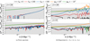 |
Fig. 3 Relative difference of the aliased with respect to the de-aliased (see Section 3.1) matter power spectrum (left panel) and bispectrum in the squeezed limit (k1 = k2 = k; k3 = kf) (right panel). In the upper panels, we show the differences for initial conditions at z = 24, and in the lower panels, the results for the final snapshot at z = 0. The results for simulations with different PNG models are shown in different colours, as indicated in the legend. The shaded areas show the 1% difference around the higher-resolution reference simulation (Section 3.3). Aliasing introduces a spurious signal in the initial conditions (upper panels) for both the power spectrum and bispectrum, reaching 3% and 10% differences, respectively, in the gNL = 107 case. By late times (z = 0), these discrepancies are suppressed to below 1% across all scales and PNG parameter values considered. |
4.2.3 Halo mass function
We now turn our attention to the halo mass functions, following the same procedure as in Section 4.1. Figure 4 shows the ratio of the halo mass functions for the different cosmologies, comparing the simulations where we have the aliasing effect with respect to the de-aliased simulations. The gravitational evolution and the process of halo finding are very non-linear, so even the tiny differences we saw in the initial conditions get amplified. This makes the halo mass function much noisier compared, for example, to the matter power spectrum that we have analysed previously. Nevertheless, we find an excellent agreement for all the cosmologies and mass ranges that are resolved with our simulations.
All the mass functions are compatible within a 3% level. This is true even for the largest mass bin, which we expect to be dominated by shot noise.
4.2.4 Halo bias
Finally, we studied the halo power spectrum and bispectrum, but this time focusing only on the fNL cosmologies. These statistics are much noisier than the matter ones due to the non-linear nature of the gravitational collapse and halo finding, as in the HMF case. In order to extract more robust conclusions, we chose to compress these statistics into 2 parameters, the halo linear bias b1 and the PNG response parameter p (defined in Equation (14)). To do this, we measured the halo power spectrum in the same way as we described in Section 4 and fitted to Equation (12) using a least squares approach. We followed the same procedure as in Avila & Adame (2022) to match the fNL = 0 realisation with the fNL = 100 (and similarly for fNL = −100) in order to suppress the variance in the measurement of bϕfNL and get more robust measurements of these parameters. We got the values for bϕ and then for p by assuming the values of fNL used to generate the initial conditions of the simulations.
The halo linear bias b1 and the PNG response parameter p (defined in Equation (14)) from the simulations summarised in Table 1, both aliased and de-aliased (see Section 3.1) are shown in Figure 5. We find that aliasing had no significant impact in either of the parameters, b1 or p. This aligns with the findings that aliasing has a small effect at late times. The only configuration that shows a larger deviation for the p parameter (although still compatible within the 1σ error bars) is 2LPT with zstart = 49. A more detailed analysis of this configuration was carried out by varying the scale cuts and the mass range considered. When applying these changes, we found that everything aligned with our observations for the remaining configurations, leading us to conclude that this was a statistical fluctuation.
We find that earlier starts led to an artificially larger value of b1, leading to a 2σ deviation for zstart = 99 when compared with our reference high-resolution simulation. These results support our findings in Section 4.1, showing that later starts with higher-order LPT improved the convergence towards the higher- resolution simulations. Regarding the p response parameter, we found that the LPT order and the initial redshift had a negligible impact.
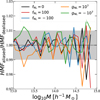 |
Fig. 4 Ratio at z = 0 of the halo mass functions from simulations affected by PNG aliasing to the de-aliased corresponding simulation (see Section 3.1). As indicated in the legend, the line colours correspond to the different PNG models used in the simulations. The shaded area represents the 1% variation around the de-aliased simulations. The PNG aliasing signal produces variations below 3% in the halo mass function at z = 0. |
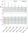 |
Fig. 5 Measurements at z = 0 of the linear bias parameter b1 (upper panel) and the PNG-response parameter p (lower panel) for halos from the simulations summarised in Table 1. The colours indicate the LPT order used for the initial conditions (red: 1LPT, green: 2LPT, and blue: 3LPT). The crosses present the best-fit values with the 1σ error bars from the fits for the simulations with a PNG aliasing signal. The circles present the results after removing the PNG alias signal, or dealiased simulations (see Section 3.1). The horizontal grey lines show the measurements from our reference high resolution simulations (see Section 3.3). The grey regions show the 1σ uncertainty from the fit to the reference simulation (Section 3.3). In the lower panel, the dashed horizontal line shows the universality relation, p = 1. |
4.3 Comparison of state-of-the-art IC-codes
We compared several public codes to generate local PNG initial conditions, namely 2LPTPNG, LPICOLA, and FastPM. To isolate differences in their PNG implementations, we initialised all runs at zstart = 49 with 2LPT and focused on fNL as we discussed in Section 3.2. Although we only show results for fNL = 100, we found similar results for fNL = −100.
4.3.1 Power spectrum
The left panel of Figure 6 shows the relative differences of the power spectrum with respect to MonofonIC at the initial redshift, z = 49, and at z = 0. 2LPTPNG and FastPM with the configuration of kmax = 1 are the codes that yielded a better agreement with respect to our reference simulation, with relative differences of 0.001% at large scales and less than 1% even at the kNyq. We noted that this increase in the differences at small scales is similar to the behaviour of the aliasing signal (left panel of Figure 3). Neither 2LPTPNG nor FASTPM kmax = 1 correct for aliasing, so we are seeing indeed the aliasing effect in these codes.
We found a residual oscillatory pattern for FastPM due to differences in the implementation of the interpolation scheme for the input power spectrum. Also, this different interpolation scheme can account for the 10−5 systematic difference between 2LPTPNG and MonofonIC as it propagates via the σ8 normalisation of the power spectrum that these codes perform.
An interesting behaviour occurs in FastPM when setting kmax = 1/4 and kmax = 2/3. There is a jump at those frequencies (we show them as vertical lines). These scales correspond to the point where all the PNG signal is removed for smaller scales for these choices of parameters in FastPM. This leads to a nearly constant offset, at a level of 0.1%, in the power spectrum due to the differences between the power spectrum in fNL = 0 and fNL = 100. Note that increasing the parameter LPT_NC_FACTOR to 2, which controls the grid size for the LPT calculations, does not modify the pass band filter kmax.
The code that shows larger variations with respect to MonofonIC is LPICOLA. The larger variations are due to the different white noise generators used in LPICOLA with respect to the reference simulation, as we explained in Section 3.2. Nevertheless, the differences are still compatible with cosmic variance and are below 1%, even at k = kNyq.
At z = 0, we found that the non-linear evolution amplified the slight differences we saw in the initial power spectrum. For 2LPTPNG and FastPM (in all the configurations), we found an excellent agreement where the differences on the power spectrum are below 0.2% at all scales. LPICOLA shows larger deviations at the level of the 1% for most scales, with only some fluctuations reaching 4% for the least sampled modes due to the differences in the white noise generator (see Section 3.2).
4.3.2 Bispectrum
We now analyse the bispectrum results. As in Section 4.2, we focused on the squeezed limit (k1 ~ k2 = k; k3 = 3kf), as most of the local PNG signal resides there, although we also checked other configurations leading to the same conclusions. The results are shown in the right panel of Figure 6. At the initial conditions, we found an excellent agreement between 2LPTPNG, FastPM (with kmax = 1 and kmax = 2/3), and MonofonIC, with marginal differences at the level of 0.1% at all scales. The ~3% variations in the bispectrum of LPICOLA were due to the differences in the white noise generator (see Section 3.2).
The largest difference occurs for FASTPM with kmax = 1/4. Although the agreement with the other codes and configurations is excellent at large scales, the low-pass filter set to ϕ2 precisely at k = 1/4 kNyq leads to a ~80% deviation for the bispectrum at smaller scales. This deviation corresponds to switching from the bispectrum for fNL = 100 (or in general, fNL ≠ 0) to fNL = 0, eliminating the entire PNG signal for smaller scales. This also has dramatic consequences for the clustering of halos, as we discuss below. The same effect would be present for FastPM with kmax = 2/3, but shifted to kcut = 2/3knyq. However, given our grid resolution and our FFT-based bispectrum estimator (see Section 3.4), we do not see this effect here for kmax = 2/3.
At z = 0, we found that the relative differences in the bispectrum for FastPM and 2LPTPNG grew to 0.09% yielding again an excellent agreement compared with MonofonIC. Moreover, the strong effect we saw for FastPM kmax = 1/4 was no longer present in the bispectrum at z = 0. This is because the gravitational evolution part dominates the bispectrum at such late times, so the local PNG bispectrum is subleading. This is not the case at high redshifts, where the bispectrum associated with gravitational evolution is significantly suppressed, and the local PNG bispectrum becomes relevant.
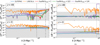 |
Fig. 6 Relative variations of the matter power spectrum (left panel) and bispectrum in the squeezed limit (k1 = k2 = k; k3 = 3kf) (right panel) with respect the reference simulation using MonofonIC (see Section 3.3). In the upper panels, we show the variations at the initial redshift, z = 49, and in the lower panels at z = 0. The codes are shown in different colours: 2LPTPNG (blue), LPICOLA (orange), FASTPM kmax = 1 (red), FastPM kmax = 2/3 (green), and FastPM kmax = 1/4 (purple). The vertical dashed lines show k = knyq × 1/4, and the vertical dash-dotted lines k = knyq × 2/3. The grey shaded regions represent 1% differences with respect to the reference. LPICOLA shows the largest variations at small k, due to a different realisation of the white noise than the reference simulation (see Section 3.2). Notably, FastPM with kmax = 1/4 shows a 80% deviation for |

4.3.3 Halo mass function
We now focus on how using different initial conditions codes may lead to differences in the clustering of halos. As in Section 4.1, the non-linear nature of gravitational evolution and halo finding amplifies the tiny differences in the initial conditions generated with the different codes, so the resulting halo mass function ratios are very noisy. Although not shown explicitly here, the results are similar to Figure 4. Simulations started with MonofonIC, FastPM, and 2LPTPNG agree in the HMF within a 1% for all the mass ranges up to 1015 h−1M⨀, with no systematic deviations. There are fluctuations for LPICOLA for Mhalo > 1014.85 h−1 M⨀, reaching the level of 12%. However, these differences are not significant as these bins are shot noise dominated, and the cosmic variance due to the different white noise generators can account for this (see Section 3.2).
4.3.4 Halo bias
To further assess the differences in halo clustering, we split the halos into four mass bins7. We followed the same strategy as in Section 4.2 and opted to compress the information in the halo power spectrum into the linear bias b1 and the PNG-response parameter p.
Figure 7 shows that all codes produced consistent b1 for all mass bins, compared to the reference simulation (see Section 3.3), which uses MonofonIC for generating the initial conditions. Even LPICOLA, with a different initial white noise, shows excellent agreement with the other codes, with only a marginal deviation of 1.1σ for the most massive bin we considered. This, in turn, is also the one most affected by the shot noise.
Regarding the PNG response parameter p, we also found an excellent agreement between MonofonIC, 2LPTPNG, LPICOLA, and FastPM (with kmax = 1 and 2/3). In particular, we found that for our mass bins, the values of p were compatible within our error bars with the universality relation p = 1.
Remarkably, FastPM with kmax = 1/4 showed a tendency to shift p above unity for low-mass halos, indicating a suppression of the scale-dependent bias signal. For high-mass halos, the agreement was again good. We traced this effect to the same scale (k ≈ kNyq/4) where the low-pass filter was applied and where we found a 80% deviation in the bispectrum of the initial conditions (see the right panel of Figure 6). This scale corresponds to a mass of roughly M ~ 300 · mpart ~ 2.4 × 10¹³ h−1M⨀. In particular, the first three mass bins were below this threshold (for which we recover p > 1 at 3σ), while for the last mass bin, all halos had a mass above this threshold.
When the kmax parameter was increased to 2/3 or 1, this artefact disappeared, as it corresponds to halo masses that are not resolved. We note that although the particular threshold in mass depends on the characteristics of the simulation, the quantity in terms of the mass of the particle is independent of the resolution. We have only analysed the results at z = 0, so it might be possible that the M ~ 300 · mpart threshold varies at higher redshifts. When using FastPM, our recommendation is to set kmax to 2/3 or 1, to avoid the spurious effects reported above.
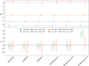 |
Fig. 7 Measurements at z = 0 of the linear bias parameter b1 (upper panel) and the PNG-response parameter p (lower panel) for different codes. All simulations have been initialised at z = 49 using 2LPT and fNL = 100 (see Section 3.2). All the points from the same code or configuration have a different marker and are grouped, from left to right, MonofonIC, 2LPTPNG,LPICOLA, and FastPM, with kmax = 1, kmax = 2/3, and kmax = 1/4. the colours indicate different halo mass bins (blue: 1.6 · 1012 < M(h−1 M⨀) < 4.0 · 1012, green: 4.0 · 1012 < M(h−1M⨀) < 8.0 · 1012, orange: 8.0 · 1012 < M(h−1M⨀) < 2.4 · 1013, and red: 2.4 · 1013 < M(h−1M⨀) < 1.3 · 1015). The horizontal dashed lines in the upper panel show the values of b1 measured in our reference simulation, using MonofonIC (Section 3.3). In the lower panel, the horizontal dashed line shows the universality relation for bϕ/p. The value of p measured from the simulation run with FastPM assuming kmax = 1/4 is ~2.7σ away from the reference for the first three mass bins (Section 4.2). The values of b1 and p measured from all other codes and configurations agree within 1σ. |
5 Summary and conclusions
We investigated methods to enhance the accuracy and efficiency of simulations that incorporate local primordial non- Gaussianities (PNG). Here, we focused on: (i) assessing how the initial redshift and LPT order influence the convergence of several statistics in the presence of local PNG; (ii) evaluating aliasing effects due to the local PNG generation; and (iii) comparing the consistency between four state-of-the-art initial condition (IC) generators for PNG, MonofonIC (which served as our reference), 2LPTPNG, FastPM, and LPICOLA. The codes are described in Section 3.2.
We produced a suite of 186 N-body simulations with different local PNG amplitudes, fNL = 0, ±100 and gNL = 0, ±107, in simulation boxes of side Lbox = 1 h−1 Gpc, assuming a Planck cosmology (see Section 3). We analysed the simulations only at their initial redshift and z = 0. We ran pairs of aliased and de-aliased simulations, using the 3/2 zero-padding technique introduced by Orszag (1971) (Section 3.1). The simulations have initial redshifts from zstart = 99 down to zstart = 11.5, and LPT orders from 1 to 3 (Table 1). For a reliable benchmark, we ran a set of reference simulations with eight times more particles, Npart = 10243 , than our baseline runs (Section 3.3).
As PNG changes the depth of the gravitational potential wells, the validity of the LPT approximation used to generate the initial conditions needed to be tested. In Section 4.1, we quantified how the initial redshift and LPT order affect the convergence of the power spectrum, bispectrum, halo mass function, halo bias, and PNG response parameter p compared with a highresolution simulation. Our results for simulations with PNG are fully consistent with those for the Gaussian case, which was already tested in Michaux et al. (2020), and are also in line with the findings from Stahl et al. (2024a) for scale-dependent PNG. Pushing to lower zstart helped reduce the effect of discreteness errors.
We find that a configuration with 3LPT and zstart = 11.5 leads to a sub-percent agreement in the power spectrum up to kNyq and in the bispectrum up to 2/3knyq. The configuration for the initial conditions has a significant impact on the halo mass function and halo bias. However, this does not affect the PNG response parameter p for halos selected by mass. Our positive and negative fNL and gNL runs show a similar behaviour at z = 0 as in the Gaussian case. Thus, given that Michaux et al. (2020) already showed that discreteness and truncation errors were larger at higher z, we expect the PNG simulations to follow the same trend as the Gaussian case at intermediate redshifts.
We quantified the aliasing signal that arises in simulations with local PNG due to the terms ϕ2 and ϕ3, in Section 4.2. We measured the PNG aliasing signal in the power spectrum, bispectrum, halo mass function, halo bias function, and PNG response parameter by comparing pairs of aliased and de-aliased simulations (Section 3.1). These pairs have the same configuration beyond the aliasing signal. The power spectrum of the initial conditions shows a scale-dependent increase. This effect is sub-percent at large scales, but becomes ~3% at kNyq for gNL = ±107. We find similar trends for the bispectrum of the initial conditions. However, after evolving at z = 0, the aliasing signal is suppressed, and it is sub-percent at all scales for all the cosmologies we considered. We do not find any significant variation associated with aliasing for the halo bias, b1, or the PNG response parameter, p. Intermediate redshifts are expected to fall between the initial and z = 0 limits. Moreover, because the aliasing signal scales linearly with the PNG amplitude, the aliasing effect would be even smaller for realistic simulations, including a smaller |fNL| or |gNL| values.
We find sub-percent agreement between the power spectrum and bispectrum (at zstart and z = 0), halo mass function, halo bias, and PNG-response parameters measured in simulations with IC generated with MonofonIC, 2LPTPNG, and FastPM with kmax = 1 (Section 4.3). Given the excellent agreement at both the initial redshift and z = 0, we expected a similar behaviour at intermediate epochs. After running all the simulations, we found that LPICOLA was producing a different realisation of the white noise when running in the GAUSSIAN mode and when running in LOCAL_FNL mode. This has complicated the one-to-one comparisons. Nevertheless, the differences found for this code were compatible with cosmic variance. If FastPM is ran with a low-pass filter for the ϕ2 field at k = kmax · kNyq, our results suggest that a value of kmax ≥ 2/3 should be used to avoid the spurious effects reported in Section 4.3.
Starting at a lower redshift with higher-order LPT improves the convergence to the fluid limit not only in Gaussian simulations (Michaux et al. 2020) but also for those with PNG. Skipping the first steps of the N-body allows more accurate and computationally efficient simulations to be run. This gain is higher if using tree codes, where typically, the first timesteps are the most expensive to run and are also the ones that can introduce more numerical errors during the force evaluations. For example, the run times of the simulations presented here with zstart = 99 were 25% longer than those that started at zstart = 11.5. The limit on pushing for a lower starting redshift must be carefully studied as it depends on the mass resolution.
The aliasing signal induced in simulations with PNG is low. Adequately removing this signal requires adding a zero-padding to the grid in Fourier space, which increases the size of the original grid by a factor of (3/2)3 , and thus increases the memory required for the computation. If resources are limited, and ~1% precision is enough, then it is safe to neglect the effect of PNG aliasing. In the future, we will explore the implementation in MonofonIC of an implicit padding algorithm to dealias IC without the extra memory cost (e.g. Bowman & Roberts 2011).
We have validated a set of PNG IC generators available to the community. Our results serve to design accurate and efficient simulations with PNG. These will be key for benchmarking analysis tools for the new-generation galaxy surveys, whose goal is to constrain inflationary physics.
Data availability
All the codes used in this paper are public. The links to the code repositories are included in footnotes in Section 3. All the simulations and data products will be shared under email request to the corresponding author.
Acknowledgements
We thank Adrian Bayer for discussions about the draft and helping with FastPM. We also thank Thomas Flöss and Raul Angulo for very useful discussions during the early elaboration of this paper. We also thank the ‘Centro de Ciencias de Benasque Pedro Pascual’ and the ‘Understanding Cosmological Observations’ workshop held within it, as they helped initiating this project. AGA gratefully acknowledges all the members of the Data Science in Astrophysics & Cosmology Group at the University of Vienna for hosting me as an intern for three months during the development of this work under the Erasmus+Prácticas programme 2023-1-ES01-KA131-HED-000116324. This work has been supported by Ministerio de Ciencia e Innovación (MICINN) under the following research grants: PID2021-122603NB-C21 (AGA, VGP, GY) and PID2021-123012NB (AGA, SA). SA has been supported by the Ramon y Cajal fellowship (RYC2022-037311-I) funded by MCIN/AEI/10.13039/501100011033 (Spain) and Social European Funds plus (FSE+). VGP has been supported by the Atracción de Talento Contract no. 2019-T1/TIC-12702 and 2023-5A/TIC-28943 granted by the Comunidad de Madrid in Spain. MM is supported by the MICINN project PID2022-141079NB-C32 The simulations presented in this paper were run in the Hydra cluster of the IFT and in Finisterrae-3 in CESGA under the project AECT-2024-3-0030. The analysis in this work has also been carried out in the computing cluster at UAM (TAURUS).
References
- Adame, A. G., Avila, S., Gonzalez-Perez, V., et al. 2024, A&A, 689, A69 [NASA ADS] [CrossRef] [EDP Sciences] [Google Scholar]
- Alam, S., de Mattia, A., Tamone, A., et al. 2021, MNRAS, 504, 4667 [NASA ADS] [CrossRef] [Google Scholar]
- Alonso Asensio, I., Dalla Vecchia, C., Potter, D., & Stadel, J. 2023, MNRAS, 519, 300 [Google Scholar]
- Angulo, R. E., & Hahn, O. 2022, Liv. Rev. Comput. Astrophys., 8, 1 [CrossRef] [Google Scholar]
- Angulo, R. E., & Pontzen, A. 2016, MNRAS, 462, L1 [NASA ADS] [CrossRef] [Google Scholar]
- Avila, S., & Adame, A. G. 2022, MNRAS, 519, 3706 [Google Scholar]
- Avila, S., Crocce, M., Ross, A. J., et al. 2018, MNRAS, 479, 94 [NASA ADS] [CrossRef] [Google Scholar]
- Babich, D., & Zaldarriaga, M. 2004, Phys. Rev. D, 70, 083005 [Google Scholar]
- Baldauf, T., Mercolli, L., Mirbabayi, M., & Pajer, E. 2015, JCAP, 2015, 007 [CrossRef] [Google Scholar]
- Ballardini, M., Matthewson, W. L., & Maartens, R. 2019, MNRAS, 489, 1950 [NASA ADS] [CrossRef] [Google Scholar]
- Barreira, A., & Krause, E. 2023, JCAP, 2023, 044 [CrossRef] [Google Scholar]
- Barreira, A., Cabass, G., Schmidt, F., Pillepich, A., & Nelson, D. 2020, JCAP, 2020, 013 [NASA ADS] [CrossRef] [Google Scholar]
- Bartolo, N., Komatsu, E., Matarrese, S., & Riotto, A. 2004, Phys. Rep., 402, 103 [NASA ADS] [CrossRef] [Google Scholar]
- Baumann, D. 2012, TASI Lectures on Inflation [Google Scholar]
- Bayer, A. E., Zhong, Y., Li, Z., et al. 2025, JCAP, 2025, 016 [Google Scholar]
- Behroozi, P. S., Wechsler, R. H., & Wu, H.-Y. 2012, ApJ, 762, 109 [Google Scholar]
- Besuner, R., Dey, A., Drlica-Wagner, A., et al. 2025, The Spectroscopic Stage-5 Experiment [Google Scholar]
- Bianchi, D., Burden, A., Percival, W. J., et al. 2018, MNRAS, 481, 2338 [Google Scholar]
- Bouchet, F. R., Juszkiewicz, R., Colombi, S., & Pellat, R. 1992, ApJ, 394, L5 [Google Scholar]
- Bouchet, F. R., Colombi, S., Hivon, E., & Juszkiewicz, R. 1995, A&A, 296, 575 [NASA ADS] [Google Scholar]
- Bowman, J. C., & Roberts, M. 2011, SISC, 33, 386 [Google Scholar]
- Byrnes, C. T., & Choi, K.-Y. 2010, Adv. Astron., 2010, 724525 [Google Scholar]
- Byrnes, C. T., Nurmi, S., Tasinato, G., & Wands, D. 2010, JCAP, 2010, 034 [Google Scholar]
- Chan, K. C., Ferrero, I., Avila, S., et al. 2022, MNRAS, 511, 3965 [NASA ADS] [CrossRef] [Google Scholar]
- Chaussidon, E., Yèche, C., de Mattia, A., et al. 2025, JCAP, 2025, 029 [Google Scholar]
- Chen, X. 2010, Adv. Astron., 2010, 638979 [NASA ADS] [CrossRef] [Google Scholar]
- Chisari, N. E., & Zaldarriaga, M. 2011, Phys. Rev. D, 83, 123505 [NASA ADS] [CrossRef] [Google Scholar]
- Creminelli, P., & Zaldarriaga, M. 2004, JCAP, 2004, 006 [CrossRef] [Google Scholar]
- Crocce, M., Pueblas, S., & Scoccimarro, R. 2006, MNRAS, 373, 369 [NASA ADS] [CrossRef] [Google Scholar]
- Dalal, N., Doré, O., Huterer, D., & Shirokov, A. 2008, Phys. Rev. D, 77, 123514 [CrossRef] [Google Scholar]
- DESI Collaboration (Aghamousa, A., et al.) 2016, arXiv e-prints [arXiv:1611.00036] [Google Scholar]
- Doré, O., Bock, J., Ashby, M., et al. 2015, Cosmology with the SPHEREX AllSky Spectral Survey [Google Scholar]
- Ereza, J., Prada, F., Klypin, A., et al. 2024, MNRAS, 532, 1659–1682 [NASA ADS] [CrossRef] [Google Scholar]
- ESA Planck Legacy Archive 2018, Baseline_params_table_2018_95pc.pdf, https://wiki.cosmos.esa.int/planck-legacy-archive/images/9/9c/Baseline_params_table_2018_95pc.pdf, accessed June 6, 2025 [Google Scholar]
- Feng, Y., Chu, M.-Y., Seljak, U., & McDonald, P. 2016, MNRAS, 463, 2273 [NASA ADS] [CrossRef] [Google Scholar]
- Fidler, C., Tram, T., Rampf, C., et al. 2017, JCAP, 2017, 022 [CrossRef] [Google Scholar]
- Forero-Sánchez, D., Rashkovetskyi, M., Alves, O., et al. 2025, JCAP, 2025, 055 [Google Scholar]
- Garrison, L. H., Eisenstein, D. J., Ferrer, D., Metchnik, M. V., & Pinto, P. A. 2016, MNRAS, 461, 4125 [NASA ADS] [CrossRef] [Google Scholar]
- Garrison, L. H., Eisenstein, D. J., & Pinto, P. A. 2019, MNRAS, 485, 3370 [CrossRef] [Google Scholar]
- Grossi, M., Verde, L., Carbone, C., et al. 2009, MNRAS, 398, 321 [CrossRef] [Google Scholar]
- Hadzhiyska, B., Garrison, L. H., Eisenstein, D. J., & Ferraro, S. 2024, Phys. Rev. D, 109, 103530 [NASA ADS] [CrossRef] [Google Scholar]
- Hahn, O., & Angulo, R. E. 2016, MNRAS, 455, 1115 [Google Scholar]
- Hahn, O., & Paranjape, A. 2016, Phys. Rev. D, 94, 083511 [Google Scholar]
- Hahn, O., Abel, T., & Kaehler, R. 2013, MNRAS, 434, 1171 [Google Scholar]
- Hahn, O., Rampf, C., & Uhlemann, C. 2020, MNRAS, 503, 426 [Google Scholar]
- Hamaus, N., Seljak, U., & Desjacques, V. 2011, Phys. Rev. D, 84, 083509 [NASA ADS] [CrossRef] [Google Scholar]
- Heinrich, C., Doré, O., & Krause, E. 2024, Phys. Rev. D, 109, 123511 [Google Scholar]
- Heitmann, K., White, M., Wagner, C., Habib, S., & Higdon, D. 2010, ApJ, 715, 104 [Google Scholar]
- Howlett, C., Manera, M., & Percival, W. J. 2015, A & C, 12, 109 [Google Scholar]
- Joyce, M., & Marcos, B. 2007, Phys. Rev. D, 75, 063516 [Google Scholar]
- Joyce, M., Marcos, B., Gabrielli, A., Baertschiger, T., & Sylos Labini, F. 2005, Phys. Rev. Lett., 95, 011304 [Google Scholar]
- Karagiannis, D., Lazanu, A., Liguori, M., et al. 2018, MNRAS, 478, 1341 [NASA ADS] [CrossRef] [Google Scholar]
- Karagiannis, D., Maartens, R., Fonseca, J., Camera, S., & Clarkson, C. 2024, JCAP, 2024, 034 [Google Scholar]
- Komatsu, E., & Spergel, D. N. 2001, Phys. Rev. D, 63, 063002 [NASA ADS] [CrossRef] [Google Scholar]
- Krause, E., Eifler, T. F., Zuntz, J., et al. 2017, arXiv e-prints [arXiv:1706.09359] [Google Scholar]
- Laureijs, R., Amiaux, J., Arduini, S., et al. 2011, arXiv e-prints [arXiv:1110.3193] [Google Scholar]
- Lazeyras, T., Barreira, A., Schmidt, F., & Desjacques, V. 2023, JCAP, 2023, 023 [CrossRef] [Google Scholar]
- Lesgourgues, J. 2011, arXiv e-prints [arXiv:1104.2932] [Google Scholar]
- Lewis, A., Challinor, A., & Lasenby, A. 2000, ApJ, 538, 473 [Google Scholar]
- LSST Science Collaboration (Abell, P. A., et al.) 2009, arXiv e-prints [arXiv:0912.0201] [Google Scholar]
- Lyth, D. H., & Wands, D. 2002, Phys. Lett. B, 524, 5 [Google Scholar]
- Lyth, D. H., Ungarelli, C., & Wands, D. 2003, Phys. Rev. D Part. Fields, 67, 2 [Google Scholar]
- Maldacena, J. 2003, JHEP, 2003, 013 [NASA ADS] [CrossRef] [Google Scholar]
- Mansfield, P., & Avestruz, C. 2021, MNRAS, 500, 3309 [Google Scholar]
- Marinucci, M., Desjacques, V., & Benson, A. 2023, MNRAS, 524, 325 [Google Scholar]
- Matarrese, S., & Verde, L. 2008, ApJ, 677, L77 [NASA ADS] [CrossRef] [Google Scholar]
- McCullagh, N., Jeong, D., & Szalay, A. S. 2016, MNRAS, 455, 2945 [Google Scholar]
- Michaux, M., Hahn, O., Rampf, C., & Angulo, R. E. 2020, MNRAS, 500, 663 [NASA ADS] [CrossRef] [Google Scholar]
- Noriega, H. E., Aviles, A., Gil-Marín, H., et al. 2025, JCAP, 2025, 136 [Google Scholar]
- Orszag, S. A. 1971, J. Atmos. Sci., 28, 1074 [NASA ADS] [CrossRef] [Google Scholar]
- Patterson, G., & Orszag, S. 1971, Phys. Fluids, 14, 2538 [Google Scholar]
- Planck Collaboration IX. 2018, A&A, 641, A9 [Google Scholar]
- Planck Collaboration VI. 2020, A&A, 641, A6 [NASA ADS] [CrossRef] [EDP Sciences] [Google Scholar]
- Pontzen, A., Slosar, A., Roth, N., & Peiris, H. V. 2016, Phys. Rev. D, 93, 103519 [NASA ADS] [CrossRef] [Google Scholar]
- Potter, D., Stadel, J., & Teyssier, R. 2017, COMPAC, 4, 2 [Google Scholar]
- Power, C., Navarro, J. F., Jenkins, A., et al. 2003, MNRAS, 338, 14 [Google Scholar]
- Rampf, C. 2012, JCAP, 2012, 004 [Google Scholar]
- Riotto, A. 2017, Inflation and the Theory of Cosmological Perturbations [Google Scholar]
- Riquelme, W., et al. 2023, Mon. Not. Roy. Astron. Soc., 523, 603 [Google Scholar]
- Ross, A. J., Banik, N., Avila, S., et al. 2017, MNRAS, 472, 4456 [NASA ADS] [CrossRef] [Google Scholar]
- Salopek, D. S., & Bond, J. R. 1990, Phys. Rev. D, 42, 3936 [NASA ADS] [CrossRef] [Google Scholar]
- Schneider, A., Teyssier, R., Potter, D., et al. 2016, JCAP, 2016, 047 [NASA ADS] [CrossRef] [Google Scholar]
- Scoccimarro, R., Hui, L., Manera, M., & Chan, K. C. 2012, Phys. Rev. D, 85, 083002 [NASA ADS] [CrossRef] [Google Scholar]
- Sefusatti, E., Crocce, M., Scoccimarro, R., & Couchman, H. M. P. 2016, MNRAS, 460, 3624 [NASA ADS] [CrossRef] [Google Scholar]
- Shiveshwarkar, C., Brinckmann, T., & Loverde, M. 2024, Constraining general multi-field inflation using the SPHEREx all-sky survey [Google Scholar]
- Slosar, A., Hirata, C., Seljak, U., Ho, S., & Padmanabhan, N. 2008, JCAP, 2008, 031 [CrossRef] [Google Scholar]
- Sousbie, T., & Colombi, S. 2016, J. Computat. Phys., 321, 644 [Google Scholar]
- Springel, V., Pakmor, R., Zier, O., & Reinecke, M. 2021, MNRAS, 506, 2871 [NASA ADS] [CrossRef] [Google Scholar]
- Stahl, C., Dubois, Y., Famaey, B., et al. 2023, JCAP, 2023, 036 [CrossRef] [Google Scholar]
- Stahl, C., Montandon, T., Famaey, B., Hahn, O., & Ibata, R. 2023, JCAP, 2023, 024 [CrossRef] [Google Scholar]
- Stahl, C., Famaey, B., Ibata, R., et al. 2024a, Phys. Rev. D, 110, 063501 [Google Scholar]
- Stahl, C., Mai, N., Famaey, B., Dubois, Y., & Ibata, R. 2024b, JCAP, 2024, 021 [Google Scholar]
- Stahl, C., Famaey, B., Ibata, R., Kraljic, K., & Castillo, F. 2025, JCAP, 2025, 042 [Google Scholar]
- Stücker, J., Hahn, O., Angulo, R. E., & White, S. D. M. 2020, MNRAS, 495, 4943 [Google Scholar]
- Sullivan, J. M., Prijon, T., & Seljak, U. 2023, JCAP, 2023, 004 [Google Scholar]
- Tellarini, M., Ross, A. J., Tasinato, G., & Wands, D. 2016, JCAP, 2016, 014 [CrossRef] [Google Scholar]
- Villaescusa-Navarro, F. 2018, Pylians: Python libraries for the analysis of numerical simulations, Astrophysics Source Code Library [record ascl:1811.008] [Google Scholar]
- Voivodic, R., & Barreira, A. 2021, JCAP, 2021, 069 [Google Scholar]
- Wagner, C., & Verde, L. 2012, JCAP, 2012, 002 [NASA ADS] [CrossRef] [Google Scholar]
- Weinberg, D. H., Mortonson, M. J., Eisenstein, D. J., et al. 2013, Phys. Rep., 530, 87 [Google Scholar]
- Zel’dovich, Y. B. 1970, A&A, 5, 84 [NASA ADS] [Google Scholar]
- Zhao, C., Chuang, C.-H., Bautista, J., et al. 2021, MNRAS, 503, 1149 [CrossRef] [Google Scholar]
1.6 1012 < M(h−1 M⨀) < 4.0 · 1012, 4.0 · 1012 < M(h−1 M⨀) < 8.0 · 1012, 8.0 · 1012 < M(h−1 M⨀) < 2.4 · 1013, and 2.4 · 1013 < M(h−1 M⨀) < 1.3 · 1015.
All Tables
Summary of the simulations ran with Npart = 5123 and Lbox = 1 h−1 Gpc, used to study the effect of LPT order, initial redshift, and aliasing in the presence of local PNG.
Parameters used to set up the initial conditions for the reference simulations for the three studies presented in this work.
All Figures
|
Fig. 1 Comparison at z = 0 of the matter power spectrum (upper panels) and bispectrum (lower panels, squeezed limit (k1 = k2 = k; k3 = 3kf)) with respect a high-resolution reference simulation (see Section 3.3). The left panel shows the results for fNL = 0 simulations, and the right panel for those with fNL = 100. The line colour encodes the LPT order used for the initial conditions (red: 1LPT, green: 2LPT, and blue: 3LPT), while the line styles indicate the initial redshift. The shaded regions indicate the ±1% around the reference simulation. The results are nearly identical for fNL = 0 and fNL = 100. A later start using higher-order LPT schemes improves the agreement with the higher-resolution reference simulations. |
| In the text | |
|
Fig. 2 Comparison at z = 0 of the halo mass function for different configurations of the initial conditions (see Section 3) with respect to the higher-resolution reference simulations (see Section 3.3). The upper panel shows the results for the fNL = 0 simulations, while the lower panel shows the case with fNL = 100. The line colour encodes the LPT order used for the initial conditions (red: 1LPT, green: 2LPT, and blue: 3LPT), while the line styles indicate the initial redshift. The dashed vertical lines show the limit of 20 particles per halo; the limit of 100 is indicated by the dash-dotted vertical lines. The shaded regions indicate the 1% difference around the reference simulation. Starting the simulation at lower redshifts improves the convergence towards the high-resolution reference. |
| In the text | |
|
Fig. 3 Relative difference of the aliased with respect to the de-aliased (see Section 3.1) matter power spectrum (left panel) and bispectrum in the squeezed limit (k1 = k2 = k; k3 = kf) (right panel). In the upper panels, we show the differences for initial conditions at z = 24, and in the lower panels, the results for the final snapshot at z = 0. The results for simulations with different PNG models are shown in different colours, as indicated in the legend. The shaded areas show the 1% difference around the higher-resolution reference simulation (Section 3.3). Aliasing introduces a spurious signal in the initial conditions (upper panels) for both the power spectrum and bispectrum, reaching 3% and 10% differences, respectively, in the gNL = 107 case. By late times (z = 0), these discrepancies are suppressed to below 1% across all scales and PNG parameter values considered. |
| In the text | |
|
Fig. 4 Ratio at z = 0 of the halo mass functions from simulations affected by PNG aliasing to the de-aliased corresponding simulation (see Section 3.1). As indicated in the legend, the line colours correspond to the different PNG models used in the simulations. The shaded area represents the 1% variation around the de-aliased simulations. The PNG aliasing signal produces variations below 3% in the halo mass function at z = 0. |
| In the text | |
|
Fig. 5 Measurements at z = 0 of the linear bias parameter b1 (upper panel) and the PNG-response parameter p (lower panel) for halos from the simulations summarised in Table 1. The colours indicate the LPT order used for the initial conditions (red: 1LPT, green: 2LPT, and blue: 3LPT). The crosses present the best-fit values with the 1σ error bars from the fits for the simulations with a PNG aliasing signal. The circles present the results after removing the PNG alias signal, or dealiased simulations (see Section 3.1). The horizontal grey lines show the measurements from our reference high resolution simulations (see Section 3.3). The grey regions show the 1σ uncertainty from the fit to the reference simulation (Section 3.3). In the lower panel, the dashed horizontal line shows the universality relation, p = 1. |
| In the text | |
|
Fig. 6 Relative variations of the matter power spectrum (left panel) and bispectrum in the squeezed limit (k1 = k2 = k; k3 = 3kf) (right panel) with respect the reference simulation using MonofonIC (see Section 3.3). In the upper panels, we show the variations at the initial redshift, z = 49, and in the lower panels at z = 0. The codes are shown in different colours: 2LPTPNG (blue), LPICOLA (orange), FASTPM kmax = 1 (red), FastPM kmax = 2/3 (green), and FastPM kmax = 1/4 (purple). The vertical dashed lines show k = knyq × 1/4, and the vertical dash-dotted lines k = knyq × 2/3. The grey shaded regions represent 1% differences with respect to the reference. LPICOLA shows the largest variations at small k, due to a different realisation of the white noise than the reference simulation (see Section 3.2). Notably, FastPM with kmax = 1/4 shows a 80% deviation for |
| In the text | |
|
Fig. 7 Measurements at z = 0 of the linear bias parameter b1 (upper panel) and the PNG-response parameter p (lower panel) for different codes. All simulations have been initialised at z = 49 using 2LPT and fNL = 100 (see Section 3.2). All the points from the same code or configuration have a different marker and are grouped, from left to right, MonofonIC, 2LPTPNG,LPICOLA, and FastPM, with kmax = 1, kmax = 2/3, and kmax = 1/4. the colours indicate different halo mass bins (blue: 1.6 · 1012 < M(h−1 M⨀) < 4.0 · 1012, green: 4.0 · 1012 < M(h−1M⨀) < 8.0 · 1012, orange: 8.0 · 1012 < M(h−1M⨀) < 2.4 · 1013, and red: 2.4 · 1013 < M(h−1M⨀) < 1.3 · 1015). The horizontal dashed lines in the upper panel show the values of b1 measured in our reference simulation, using MonofonIC (Section 3.3). In the lower panel, the horizontal dashed line shows the universality relation for bϕ/p. The value of p measured from the simulation run with FastPM assuming kmax = 1/4 is ~2.7σ away from the reference for the first three mass bins (Section 4.2). The values of b1 and p measured from all other codes and configurations agree within 1σ. |
| In the text | |
Current usage metrics show cumulative count of Article Views (full-text article views including HTML views, PDF and ePub downloads, according to the available data) and Abstracts Views on Vision4Press platform.
Data correspond to usage on the plateform after 2015. The current usage metrics is available 48-96 hours after online publication and is updated daily on week days.
Initial download of the metrics may take a while.