| Issue |
A&A
Volume 705, January 2026
|
|
|---|---|---|
| Article Number | A169 | |
| Number of page(s) | 20 | |
| Section | Extragalactic astronomy | |
| DOI | https://doi.org/10.1051/0004-6361/202556291 | |
| Published online | 16 January 2026 | |
Introducing NewCluster: First half of the history of a high-resolution cluster simulation
1
Institut d’Astrophysique de Paris, Sorbonne Université, CNRS, UMR 7095 98 bis bd Arago 75014 Paris, France
2
Department of Astronomy and Yonsei University Observatory, Yonsei University Seoul 03722, Republic of Korea
3
Korea Astronomy and Space Science Institute, 776, Daedeokdae-ro Yuseong-gu Daejeon 34055, Republic of Korea
4
Korea Institute of Advanced Studies (KIAS), 85 Hoegiro Dongdaemun-gu Seoul 02455, Republic of Korea
5
Kyung Hee University, Dept. of Astronomy & Space Science Yongin-shi Gyeonggi-do 17104, Republic of Korea
★ Corresponding authors: This email address is being protected from spambots. You need JavaScript enabled to view it.
; This email address is being protected from spambots. You need JavaScript enabled to view it.
Received:
7
July
2025
Accepted:
17
November
2025
Abstract
Aims. We introduce NEWCLUSTER, a novel high-resolution cluster simulation designed to serve as the massive halo counterpart of the modern cosmological galaxy evolution framework.
Methods. The zoom-in simulation targets a volume of 4.1σ overdensity region, which is expected to evolve into a galaxy cluster with a virial mass of 5 × 10¹⁴ M⊙, comparable to that of the Virgo Cluster. The zoom-in volume extends out to 3.5 virial radii from the central halo. The novelties of NEWCLUSTER are exemplified by its resolution. Its stellar mass resolution of 2 × 10⁴ M⊙ is effective for tracing the early assembly of massive galaxies as well as the formation of dwarf galaxies. The spatial resolution of 68 parsecs in the best-resolved regions in the adaptive-mesh-refinement approach is a powerful tool for studying the detailed kinematic structure of galaxies. The time interval between snapshots is also exceptionally short (i.e., 15 Myr). This is ideal for monitoring changes in the physical properties of galaxies, particularly during their orbital motion within a larger halo. The simulation includes up-to-date feedback schemes for supernovae (SNe) and active galactic nuclei (AGNs). The chemical evolution is calculated for ten elements, along with dust calculation that includes the formation, size change, and destruction. To overcome the limitations of the Eulerian approach used for gas dynamics in this study, we employed Monte Carlo-based tracer particles in NEWCLUSTER, enabling a wide range of scientific investigations.
Results. The simulation has passed z = 0.8, covering well over half of its cosmic history. We released the early data with the expectation they will facilitate studies of the early evolution of galaxies and overdensities.
Key words: hydrodynamics / methods: numerical / dust / extinction / galaxies: clusters: general / galaxies: evolution / galaxies: formation
© The Authors 2026
 Open Access article, published by EDP Sciences, under the terms of the Creative Commons Attribution License (https://creativecommons.org/licenses/by/4.0), which permits unrestricted use, distribution, and reproduction in any medium, provided the original work is properly cited.
This article is published in open access under the Subscribe to Open model. This email address is being protected from spambots. You need JavaScript enabled to view it. to support open access publication.
1. Introduction
Numerical simulations have become an indispensable tool in modern astronomy for exploring the complex and nonlinear nature of the Universe. A pioneering study by Toomre & Toomre (1972), which modeled the morphologies of interacting galaxies, demonstrated the potential of numerical simulations to capture such nonlinearity. Since then, continuous advancements in computational methods have established numerical methods as an important complement to observational and theoretical approaches (e.g., White & Rees 1978; Davis et al. 1985; Hernquist 1987; Cole 1991; White & Frenk 1991; Kauffmann et al. 1993).
These early successes have laid the foundation for the advancement of contemporary cosmological simulations. The cosmological principle assumes that both the spatial distribution of matter and its power spectrum approach homogeneity on sufficiently large scales. This justifies the use of a large numerical volume to approximate a representative subregion of the Universe. On this basis, cosmological simulations can be initialized with primordial density fluctuations consistent with the early Universe and evolved forward in time using the governing equations of gravity and hydrodynamics, coupled with astrophysical subgrid models. These calculations yield the formation and evolution of self-consistent large-scale structure within the simulated volume (e.g., Peebles 1982; Davis et al. 1985; White et al. 1987).
The observational validation of the Λ cold dark matter (ΛCDM) cosmology, including precise measurements of cosmological parameters (e.g., Komatsu et al. 2011), has significantly accelerated the development of early cosmological numerical simulations. A prominent example is the MILLENNIUM simulation (Springel et al. 2005) based on the ΛCDM model, which has successfully reproduced large-scale structures consistent with survey observations (Springel et al. 2006). This achievement sets the stage for practically attainable theoretical investigation of nonlinear cosmological structures. Although the simulation itself included only collisionless dark matter (DM) particles, subsequent studies incorporated semi-analytic models to populate galaxies, demonstrating an important link between the nonlinear nature of the Universe and galaxy evolution (e.g. Bower et al. 2006; De Lucia & Blaizot 2007).
The next generation of cosmological simulations have incorporated hydrodynamics to model baryonic physics, including cooling and heating, star formation, and feedback, through dedicated astrophysical prescriptions. Seminal large-volume simulations that pioneered this approach include EAGLE (Schaye et al. 2015), HORIZON-AGN (Dubois et al. 2014a), and ILLUSTRIS (Vogelsberger et al. 2014b). These simulations have typically achieved spatial resolutions of ∼1 kpc, sufficient to capture the global properties and statistical trends of galaxy populations in cosmological contexts (Vogelsberger et al. 2014a; Furlong et al. 2015; Dubois et al. 2016). The larger volumes further allowed for systematic studies of environmental effects on galaxy evolution by treating the environment as a controllable parameter (e.g., Jeon et al. 2022). However, a resolution of ∼1 kpc remains insufficient to resolve the internal structure and processes with sub-kiloparsec (sub-kpc) physical scales within galaxies. For example, in a Milky Way-like galaxy with a size of ∼10 kpc, only a few resolution elements are available to represent its internal structure.
Recent cosmological simulations have reached the sub-kpc resolution (e.g., Tremmel et al. 2017; Pillepich et al. 2019). With this improvement in resolution, galactic substructures begin to be resolved in a cosmological context (e.g., Du et al. 2021), enabling detailed analyses of the kinematic and spatial properties of galactic components. These sub-kpc simulations have also resolved structures beyond galaxies themselves, such as the circumgalactic medium (CGM; e.g., Peeples et al. 2019), making it feasible to study the baryon cycle of galaxies. However, despite these advances, it is sometimes insufficient to resolve finer galactic structures, such as the multiphase nature of interstellar medium (ISM) or the thin disc of spiral galaxies.
Subsequent cosmological hydrodynamic simulations have pushed the resolution below ∼100 pc (e.g., Wang et al. 2015; Wetzel et al. 2016; Dubois et al. 2021; Yi et al. 2024), with some achieving resolutions as fine as sub-10 pc (Hopkins et al. 2018b). This level of spatial resolution enables resolving both the distinction of thin and thick discs of galaxies (e.g., Park et al. 2021; Renaud et al. 2021; Yi et al. 2024) or compact systems (Jang et al. 2024) and the multiphase structure of galactic gas, including the warm and cold ISM (Dubois et al. 2021). Such high resolution has facilitated the implementation of more advanced subgrid models. Mechanical supernova feedback, which has been reported to be more effective in suppressing star formation in low-mass galaxies, has been implemented in several high-resolution simulations, enabled by the ability to assign momentum to gas elements in the immediate vicinity of star particles (Kimm & Cen 2014; Hopkins et al. 2018a). Direct measurements of the differential velocity within the ISM have been used to implement the gravo-thermo-turbulent model of star formation efficiency (Kimm et al. 2017; Kretschmer & Teyssier 2020), allowing detailed investigations on star formation activity within galaxies (Kraljic et al. 2024).
Furthermore, the corresponding increase in baryonic (and DM) mass resolution is also important, as poor resolutions introduce numerical biases (e.g., Klypin et al. 1999; Ludlow et al. 2019). Fine mass resolutions allow for the detection of structures with extremely low surface brightness, such as intracluster light (ICL), ultra-diffuse galaxies (UDGs), tidal streams, and ultra-faint dwarfs. A stellar particle mass of ∼104 M⊙ enables the simulation to reach surface brightness levels as faint as 34 mag arcsec−2 at z = 0.1. This is enough to reproduce results from deep imaging surveys such as the Large Synoptic Survey Telescope (LSST), Euclid, and the James Webb Space Telescope (JWST; see Euclid Collaboration: Borlaff et al. 2022).
Therefore, more realistic and advanced cosmological simulations at the current stage require a sub-100 pc resolution and a high mass resolution. A major challenge arising from these requests is the high computational cost due to the enormous number of elements and associated calculations. A good bypass to satisfy the needs above and to avoid this difficulty is running a simulation for a small interested region with high resolutions, while the rest of the volume is treated with relatively poorer resolutions, namely, by adopting a zoom-in approach (e.g., Navarro & White 1994; Barnes et al. 2017; Choi & Yi 2017; Hopkins et al. 2018b; Tremmel et al. 2019; Dubois et al. 2021).
The majority of recent high-resolution (sub-100 pc) zoom-in simulations focus on individual galaxies or average-density fields of the Universe. This has resulted in a lack of representative high-resolution counterparts for dense environments such as galaxy clusters. Galaxy clusters are thought to have formed from the growth of primordial over density in the early Universe (Kravtsov & Borgani 2012), implying that developing clusters were once among the most active sites of star formation (Jeon et al. 2022). Therefore, protoclusters are the primary candidates for the sites for containing high-redshift galaxies that are frequently detected by JWST (Labbé et al. 2023; Carniani et al. 2024).
In this regard, we initiated the NEWCLUSTER simulation, a high-resolution cosmological hydrodynamic simulation designed to reproduce the formation and evolution of a galaxy cluster down to near-local redshift. NEWCLUSTER serves as a massive halo counterpart to existing high-resolution zoom-in simulations on average-density fields, NEWHORIZON and NEWHORIZON2, particularly because it shares many of its subgrid prescriptions with them. The simulation aims to monitor the formation and evolution of a massive cluster and galaxy evolution inside the extreme environment.
We expect morphological transformations of galaxies in clusters, which are responsible for the prevalence of early-type galaxies with old stellar populations (Dressler 1980; Lewis et al. 2002; Hogg et al. 2004; Kauffmann et al. 2004). This transition is thought to be triggered by the interplay of both internal and external processes. The energy and outflows released by stellar activity and central supermassive black holes are considered major factors in the quenching of star formation (Murray et al. 2005; Teyssier et al. 2011). The released gas forms the hot intracluster medium (ICM), which in turn drives an external quenching process for cluster members. Moving at very fast orbital velocity (∼103 km s−1), galaxies experience rapid gas stripping through hydrodynamic ram pressure and DM and stellar stripping through gravitational tidal interactions (Smith et al. 2016; Rhee et al. 2017; Han et al. 2018; Jung et al. 2018). Such processes are likely also responsible for jellyfish galaxies (Chung et al. 2009) and possibly ultra-diffuse galaxies as well (van Dokkum et al. 2015). To closely trace the gravitational and hydrodynamic interactions that impact galaxy evolution, it is essential to achieve sufficient spatial resolution to resolve the kinematics and structural properties of galaxies. Such a level of detail was previously unavailable in prior simulations of galaxy clusters.
The impact of the cluster merger (starting at z = 0.8) is also open to wild speculations. While NEWCLUSTER lacks the capability for statistical analysis, its high spatial resolution offers the opportunity to examine the merging process in greater detail. This is particularly relevant to exploring how member galaxies are affected by the global redistribution of the gravitational mass and ICM.
In this paper, we summarize the results of the NEWCLUSTER simulation up to z = 0.8, which corresponds to the half of the age of the universe and represents the latest available snapshot. At this redshift, a halo with a mass comparable to that of a galaxy cluster is present, which enables the simulation to reproduce the formation of an observed galaxy cluster analogue and its associated phenomena. This paper is organized as follows. In Sect. 2, we describe the simulation code, astrophysical prescriptions, and post-processing methods. In Sect. 3, we present a general overview of the simulation and the galaxy scaling relations at z = 0.8, along with key examples of applications of the cluster simulation to various topics. In Sect. 4, we summarize the main findings of the paper.
2. Methods
2.1. Code: RAMSES-yOMP
RAMSES (Teyssier 2002) is an astrophysical simulation code based on the adaptive mesh refinement (AMR) technique. In this study, we used a specialized branch of the code, called RAMSES-yOMP (Han et al. 2025), which has been extensively modified to enhance simulation performance. The improvement is primarily attributed to the implementation of a hybrid parallelization scheme that utilizes a dual-level multiprocessing structure to enhance the parallel scalability, combining the message passing interface (MPI) and open multiprocessing (OMP) libraries. A series of modifications to yOMP are described in Han et al. (2025), including updates on subroutines such as the load-balancing scheme and the conjugate gradient Poisson solver, aimed at improving the overall performance of the simulation. Load balancing is enhanced by assigning greater computational weights to particles that require more processing, particularly those involved in complex feedback and density estimation. In a test suite simulating a cosmological volume with 1536 computing cores, the modified code achieved approximately a two times speed-up compared to the pre-modified version.
2.2. Initial condition and zoom-in region
The initial condition was generated using MUSIC (Hahn & Abel 2011) at z = 50 with the WMAP7 cosmology (Komatsu et al. 2011) with parameters ΩΛ = 0.728, Ωm = 0.272, σ8 = 0.810, ns = 0.967, h0 = 0.703, and Ωb = 0.0455. The transfer function from Eisenstein & Hu (1998) and CAMB (Lewis et al. 2000) is used to derive the initial distribution of DM and baryons, respectively. The zoom-in technique is utilized to efficiently simulate cluster regions in high resolution. First, we ran DM-only simulations of a box with a volume of (100 h−1 Mpc)3 with periodic boundary conditions. We used the Rockstar halo finder (Behroozi et al. 2013b) to detect halos within the volume at z = 0. Since the simulation was performed on only one galaxy cluster, we ran 15 DM-only simulations in total and selected one target halo based on visual inspection. We selected the target cluster whose evolution matches the following criteria: 1. a cluster in a relaxed state at z = 0, without ongoing major mergers; 2. a cluster that had experienced a major merger during its assembly phase.
A spherical region centred on the density peak of the target cluster was set with a radius of 3.5Rvir, where Rvir refers to the virial radius1 of the target cluster, to record the identity of the confined particles and trace their initial distribution at z = 50. The zoom-in region, corresponding to a 4.1σ overdensity above the Universal mean, is defined as a convex hull generated based on the distribution of the recorded particles in the initial volume. The selected convex hull roughly covers a comoving volume of 23 300 Mpc3 with a total mass of 8.6 × 10¹⁴ M⊙.
The volume within the zoom-in region is initialized with grids and particles with a base level of 12, the scale that corresponds to the side length of the box divided into 212 cells. This corresponds to an initial spacing of 34.7 kpc in comoving units. Padding grids are deployed around the finest zoom-in region to provide a gradual transition in resolution. This results in a continuously decreasing level of refinement in grids and an increasing mass of DM particles, from the finest level of 12 at the centre to coarser levels further away from the zoom-in region, reaching the minimum level of 8.
A single DM particle is placed in each cell with a slight offset from the centre to account for the density distribution of the initial condition. At level 12, DM particles have a mass of ∼1.3 × 10⁶ M⊙, and increase by a factor of eight as their initially placed refinement level decreases by one. As the simulation progresses, DM particles with lower refinement levels may reach inside the zoom-in region, which could impact the galaxies near the outskirts of the zoom-in region, leading to potential inconsistencies in the computation of gravitational potential and refinement. To address this, we impose our own criteria for the fraction of low-level DM particles (i.e., contamination) to exclude affected galaxies (see Sect. 2.4).
We also assigned an extra passive scalar variable to the hydro information in cells, indicating a refinement mask, which is set to 1 within the zoom-in region and 0 elsewhere. Grids with refinement masks greater than 0.05 are considered to be within the zoom-in region and become targets for refinement to higher resolution, as well as the application of baryonic physics such as star formation and active galactic nucleus (AGN) feedback.
The best spatial resolution, namely, the minimum cell size within the zoom-in region, depends on the scale factor of the simulation. This is because the simulation grid size is built based on the comoving units. To maintain physical resolution, we allow an additional level of refinement for cells each time the scale factor doubles, that is, at the transition epochs a = 0.1, 0.2, 0.4, and 0.8, effectively unlocking finer spatial resolution at these epochs. This results in a slightly different cell size depending on the current scale factor of the simulation, corresponding to a physical size of 53–107 pc. At z = 0, the simulation achieves a final resolution of 68 pc, corresponding to a grid level of 21.
The sudden increase in resolution at the specific scale factors could introduce numerical artifacts in the gas properties of galaxies. To mitigate this effect, we smoothed out the transitions at which the refinement would be applied. We followed the approach of Snaith et al. (2018), but additionally applied the same method to the Jeans length criterion. During the transition phase, we continuously varied the parameter Njeans from 0 to 1 and mrefine from 100 to 8, at the transition phase to perform smooth refinement, i.e.
![Mathematical equation: $$ \begin{aligned} C = C_{L} + \frac{1}{2}\left[1+\sin \left(\frac{(a - a_{0})\pi }{2w}\right)\right]\left(C_R-C_L\right), \end{aligned} $$](/articles/aa/full_html/2026/01/aa56291-25/aa56291-25-eq1.gif) (1)
(1)
where a is the current scale factor, a0 is the centre of the transition phase (defined as 0.1, 0.2, 0.4, 0.8 at grid levels 18, 19, 20, 21), and w is the half-width of the transition phase, set to 0.025 in this work. C is the refinement threshold and can be either NJeans or mrefine, where CL and CR denote the initial and final values for the refinement transition, respectively. The parameter pair [CL, CR] is set to [0, 1] for NJeans, and [100, 8] for mrefine. Here, mrefine defines the mass increase required for a cell to be refined. For example, if mrefine = 8, the mass within a cell needs to be eight times higher than the initial cell mass to be eligible for refinement. NJeans is the parameter for the Jeans length refinement criterion, in which the cell with a hydrogen gas density n ≥ 5 H cm−3 can be refined if
 (2)
(2)
where lJeans is the thermal Jeans length of the cell, and Δx is the current size of the cell. With this formula, cells with the shortest Jeans length, typically corresponding to the densest cells in a galaxy, are preferentially refined during the transition phase within a scale factor window of 0.05.
Since DM particles have considerably higher mass than baryonic components, the shot noise could introduce numerical artifacts in gravity calculations. We set an upper limit on the contribution of DM density on the mesh at level 18, which corresponds to the comoving resolution of 0.54 kpc.
2.3. Astrophysical prescriptions
2.3.1. Stellar physics and chemical evolution
The star formation rate (SFR) in the simulation is calculated based on the gravo-thermo-turbulent model of Kimm et al. (2017) without applying the turbulent Jeans length criterion, thereby preserving scale invariance, as in Dubois et al. (2021). The exact formation efficiency follows the equation of the multi-ff PN model (Federrath & Klessen 2012, see also Padoan & Nordlund 2011). In each time step, the amount of stellar mass formed is checked within each gas cell above a star formation density threshold of n★ = 5 H cm−3 to form a star particle.
Star particles are probabilistically formed according to a Poisson distribution. The mean of the distribution is set by the SFR integrated by time, divided by the minimum mass, 2.49 × 10⁴ M⊙. Consequently, the initial mass of each star particle is an integer multiple of this minimum mass. The mass of a star particle may decrease over time due to mass ejection during its feedback processes, with up to ∼40% of its initial mass being ejected to the surrounding medium.
The stellar feedback in the simulation consists of two kinds: supernovae (SNe) and stellar winds. The SN feedback is implemented as two independent types, Type II and Type Ia (as SNII and SNIa, respectively), both of which are implemented as the form of mechanical feedback scheme of Kimm & Cen (2014) that takes account of the empirical boost depending on the local density of the explosion (Kimm et al. 2017). Every star particle that has reached the age of 5 Myr triggers the SNII explosions. The produced feedback energy per mass is set to be eSNII = 0.045 × 1051 erg M⊙−1.
The frequency of SNIa is set to follow the delay time distribution (DTD) in the form of a power law (Maoz et al. 2012),
 (3)
(3)
where the power index is fixed to be α = −1 and the amplitude is chosen to be ϕ = 2.35 × 10⁻⁴ M⊙−1. The value of DTD amplitude ϕ is derived as a result of the normalization of the lifetime frequency of NSNIa/MSSP = 0.0013 M⊙−1 for a given simple stellar population of mass MSSP, assuming that it is integrated over the domain of 0.05 − 13.7 Gyr. The feedback energy of a single SNIa is set to 1051 erg.
For a realistic production of chemical elements within galaxies, we have included mass return from stellar ejecta of SNe type II and Ia, and stellar winds in the simulation. Throughout the simulation, we assume a Chabrier (2003) initial mass function for the integration of chemical yield from the stellar population. Considering each stellar particle as a simple stellar population (SSP), chemical enrichment for ten species (H, D, He, C, N, O, Mg, Fe, Si, and S) is computed using the Starburst99 code (Leitherer et al. 1999, 2014)2. Yields from stellar winds are derived assuming the Geneva stellar wind model (Schaller et al. 1992; Maeder & Meynet 2000). At the same time, energy produced from stellar wind is directly injected into the grid where the star is positioned. SNII explosions also inject newly synthesized elements into surroundings based on the tabulated value for the SNII yields in Kobayashi et al. (2006), assuming that each SSP has the progenitor mass range of 8 − 50 M⊙, which corresponds to the ejecta mass fraction for each stellar particle is Mejecta/M* = 0.311. The yield from SNIa is derived from Iwamoto et al. (1999) with the mass of the ejecta in every burst corresponding to the Chandrasekhar limit (∼1.4 M⊙), with corresponding decline of mass in each stellar particle.
2.3.2. Dust formation and evolution
The simulation also computes dust formation and evolution that evolves on-the-fly throughout cosmic time. The dust model implemented for NEWCLUSTER is based on that described in Dubois et al. (2024), who we refer to for further technical details, and accounts for several key physical processes, including dust formation, growth, destruction, and size evolution. Here, we provide a brief summary of the methodology.
Dust grain species are modeled with two distinct characteristic chemical compositions: carbonaceous and silicate grains. We assume that silicate grains consist of a single form of amorphous olivine, with compound MgFeSiO4, and that carbonaceous grains are composed purely of carbon. To follow the grain size distribution of dust, the two different chemical compositions are further decomposed into two different grain sizes (adopting the two-size bin approximation of Hirashita 2015) of radius 5 nm for small grains and 0.1 μm for large grains.
For dust grain production, we assume two channels: the formation from the stellar ejecta and growth through the accretion of gas-phase metals in the ISM. We consider the dust production from SNe type II and Ia, and asymptotic giant branch (AGB) winds based on the feedback models and stellar yields described above with different dust condensation efficiencies that depend on the stellar origin and on the C/O ratio (see Dubois et al. 2024 for the exact values). Accretion of gas-phase metals onto dust grains in dense and cold ISM regions is also implemented as a subgrid model. Dust accretion rates are estimated based on the gas density, temperature, and metallicity in each gas cell and depend on the grain size and its material density (sgr = 3.3 and 2.2 g cm−3 for silicate and carbonaceous grains respectively). The local gas velocity dispersion is used to sample a subgrid log-normal shape of the probability density function of the gas density, assuming isothermal turbulence. We assume that the gas-phase accretion occurs only for (subgrid) gas densities lower than nthr = 104 H cm−3, considering the formation of ice mantles on grain surfaces, which inhibit metal accretion onto pre-existing grain cores (Cuppen & Herbst 2007; Hollenbach et al. 2009). The Coulomb enhancement factor, which accounts for the electrostatic effects acting differently on various grain species, is not included in the NEWCLUSTER dust model. For dust destruction, we included thermal sputtering and supernova-driven destruction from both Ia and II explosions with increased efficiencies with decreasing grain sizes. The thermal sputtering timescale with temperature is estimated following Tsai & Mathews (1995). The SNe destroy the enclosed dust until the shock velocity decreases below the activation threshold of 100 km s−1, with identical destruction efficiencies for graphite and silicate grains. Astration completely destroys the dust engulfed in the star formation process.
The two grain sizes of each grain chemical composition can exchange mass by shattering and coagulation, respectively, decreasing and increasing the grain sizes. Shattering operates at intermediate gas densities (n ≲ 10 H cm−3) where grain turbulent velocities (σgr ≳ 10 km s−1) are sufficiently high to fragment the grains (Jones et al. 1996; Yan et al. 2004). In contrast, coagulation takes place in the dense gas phase (n ≳ 100 H cm−3) where turbulence is sufficiently low (σgr ≲ 1 km s−1) to preserve the grain structure and to allow grain size growth by collisions (Chokshi et al. 1993; Poppe & Blum 1997). The shattering and coagulation timescales are calculated following Granato et al. (2021) and Aoyama et al. (2017), respectively. Throughout the simulation, the dust components are advected with the gas flow, behaving as passive scalars. Readers are referred to Dubois et al. (2024) for further details.
2.3.3. Massive black hole physics
For AGN feedback, we employ the dual mode feedback scheme including the spin-evolution of massive black holes (MBHs) (Dubois et al. 2012, 2014b, 2021). We set the thermal feedback efficiency for the AGN to 0.05, which is three times lower than in Dubois et al. (2021). This reduces the amount of feedback energy released per unit accreted mass in quasar mode, thereby promoting black hole growth and increasing their mass at a given stellar mass, which was underestimated in previous simulations relative to observations. The formation criterion of seed MBHs is applied based on the gas and stellar properties in each cell. The target cell should have a gas density higher than nBH = 100 H/cm−3 and a stellar mass within the cell higher than 1.88 × 10⁷ M⊙. This corresponds to a density of 2500 H cm−3 at the best spatial resolution at z = 0. The motivation for using the stellar mass of the cell instead of its density is to make the occurrence frequency of peak-stellar-density cells independent of spatial resolution. Since NEWCLUSTER employs a time-dependent minimum spatial resolution, this approach helps the formation of seed black holes to be more uniformly distributed throughout the epochs. We also require the stellar velocity dispersion to be σ* > 50 km s−1 and the stellar age to be t* > 50 Myr to avoid selecting short-lived young clumps as seed MBH formation sites.
The exclusion radius, which is the radius of the spherical region that prevents the formation of new MBH around the pre-existing MBH, is set to be 4 kpc. This constraint was originally imposed to prevent the overproduction of seeds inside a single galaxy when the formation criterion was easily met. Compared to previous RAMSES simulations, our threshold scheme ensures the formation site of seeds to be reliably dense stellar concentrations that last long enough, making a large exclusion radius (e.g., 50 comoving kpc in Dubois et al. 2021) unnecessary. Our choice of 4 kpc is enough to prevent the formation of multiple seeds near the galactic centre.
Dynamical friction of MBHs (Chandrasekhar 1943; Ostriker 1999) is implemented for gas from Dubois et al. (2014b) and stars from Pfister et al. (2019). We find that seed-mass MBHs do not settle with their own dynamical friction, even when they are near the central region of the galaxy, resulting in permanent oscillation near the galaxy centre. This issue has also been reported in other simulations (Ma et al. 2021; Bahé et al. 2022). To alleviate the problem, artificial acceleration and repositioning of the MBH have been utilized, for example, by boosting dynamical friction or the accretion rate of the MBH by a factor that depends on the gas density (Weinberger et al. 2017; Wellons et al. 2023; Tremmel et al. 2018; Dubois et al. 2021).
MBHs seem to show stable settling even in higher-resolution simulations that take into account dynamical interactions with both the stars and the gas components within the Bondi-Hoyle radius (Pfister et al. 2019; Lescaudron et al. 2023; Li et al. 2025). Other simulations address stellar systems associated with the MBH (e.g., nuclear star clusters) as a critical player for the settling of the MBH (Biernacki et al. 2017; Ogiya et al. 2020; Mukherjee et al. 2025; Zhou et al. 2025; Shin et al. 2025). Since our 68 pc spatial resolution is not enough to capture these behaviors, we applied a mild boost factor on the stellar dynamical friction of the MBH,
![Mathematical equation: $$ \begin{aligned} f_{\rm boost} = \max [(\rho _*/\rho _{\rm crit})^{\beta }, 1] ,\end{aligned} $$](/articles/aa/full_html/2026/01/aa56291-25/aa56291-25-eq4.gif) (4)
(4)
where we set β = 1 and ρcrit = 0.16 M⊙ pc−3. This is based on the understanding that the enhanced drag force results from unresolved high-density regions in the subgrid regime, which enables seed-mass MBHs to remain bound to concentrated stellar systems. This binding supports their gas accretion and their early settlement at the galaxy centre by effectively deepening the gravitational potential of the system.
2.3.4. Heating and cooling of gas
The general radiative heating and cooling model follows the framework of Dubois et al. (2021). The simulation employs a UV background from Haardt & Madau (1996) with a reionization redshift of zreion = 10. Gas with density n > 0.01 H cm−3 (Rosdahl & Blaizot 2012) has a reduced UV photo-heating rate due to self-shielding by a factor of exp[−nH/(0.01 Hcm−3)]. We used tabulated cooling rates from Sutherland & Dopita (1993) and Dalgarno & McCray (1972) that vary with the metallicity, which is defined as the sum of the abundances of all gas-phase elements excluding H, He, and D.
The simulation includes an additional cooling effect from collisional interactions between electrons and dust grains at high temperature. We adopted the cooling rates from Dwek & Werner (1981), which depend on the gas temperature, dust grain size, and the number densities of hydrogen and electrons, assuming that the gas is fully ionized. The dust contribution to the gas cooling rate significantly decreases below ∼106 K, thereby preventing dust from affecting the contraction of cold gas at lower temperatures (see Dubois et al. 2024 for details).
2.4. Halo and galaxy detection
Galaxies and halos are identified separately using the AdaptaHOP algorithm (Aubert et al. 2004; Tweed et al. 2009). This method detects peaks and saddle points in the particle density field, which are used to estimate the initial centres and boundaries of halos. To build a substructure hierarchy, we adopt the “most massive sub-node method”, which regards the most massive (leaf) substructures as the central part of the host halo while other substructures inside the host halo are classified as “subhalos” (see Tweed et al. 2009 for details). The minimum number of particles is set to 100, corresponding to ∼106 M⊙ and ∼108 M⊙ for galaxies and halos, respectively. In total, 5570 galaxies and 89 994 halos are identified at z = 0.8. However, as the zoom-in simulation contains DM particles with different resolutions, some halos are contaminated by low-resolution particles. To consider this, we applied a strict condition that excludes halos with at least one poor-resolution DM particle, resulting in 73 745 halos in total. The mass ranges are 106.26 − 12.12 M⊙ for galaxies and 108.12 − 14.15 M⊙ for halos. The two most massive halos, which are merging at z = 0.8, also satisfy this condition and contain no low-resolution DM particles.
Furthermore, we excluded transient and star-forming clumps from our galaxy sample. Such clumps are often identified as substructures within galaxies, lack both longevity and clear visual distinction from the main galaxy in their stellar distributions, and are incorporated into their main host. These clumps are defined by the following criteria: 1. they are substructures of the host group; and 2. their main progenitor branch persists for fewer than 100 snapshots (i.e., 1.5 Gyr) or they appear as substructures in over 90% of all snapshots.
Although AdaptaHOP computes several main halo properties such as virial radius3 or spin parameter, we further calculated key quantities related to stellar or gas components. To measure these quantities, we applied different strategies for stellar and gas properties. For stellar properties of a galaxy (e.g., SFR or metallicity), we only considered member particles identified by the galaxy finder. On the other hand, gas properties (e.g., gas mass) were measured using several radius cuts, such as the stellar half-mass radius R50, 3D (or R90, 3D), which is the three-dimensional (3D) radius within which a galaxy contains 50% (90%) of its stellar mass, and Rmax, the distance from the centre to the farthest member particle. We publicly provide all value-added catalogues on the simulation website4.
3. Results
3.1. Overview of the simulation
The simulation has passed z = 0.8 which corresponds to 6.9 Gyr after the Big Bang. In total, 459 valid snapshots were exported with time intervals of 15 Myr. At z = 0.8, the zoom-in region includes 19 galaxies with M* > 1011 M⊙, 170 galaxies with M* > 1010 M⊙, and 801 galaxies with M* > 109 M⊙. The main cluster has a total mass of M200 = 1.2 × 10¹⁴ M⊙, and is in the beginning stage of a merger with a smaller halo of M200 = 2 × 10¹³ M⊙. This is a major merger, as the mass ratio was 1:3.2 when the secondary halo had its peak mass at z = 0.91. Figure 1 presents the images of the simulation volume at four different scales: (a) the entire simulation box including low-resolution regions, (b) the zoom-in region, (c) the most massive galaxy cluster, and (d) the central galaxies of the target galaxy cluster. The color scheme represents the various components of the simulation, as shown by the legends at the top left of each panel. The figure also shows the same region at four additional redshifts, z = 1.0, 1.5, 2.5, and 4.0, in panels (e) through (h), each rendered at a fixed physical scale. These panels reveal the development of large-scale structure, with galaxies as building blocks, that eventually merge into the central halo to form a cluster, as well as the hot gas bubbles and reservoirs generated by stellar and AGN feedback.
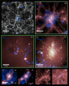 |
Fig. 1. Overview of the NEWCLUSTER simulation. The figure shows images of (a) the large-scale volume that includes a low-resolution region, (b) the zoom-in region that includes clusters and local gas filaments, (c) the main cluster and infalling galaxies, and (d) the central brightest cluster galaxy with a relatively massive companion on the lower right side. Each panel shows a different combination of components that are specified on the upper left side with their corresponding colors. The extent of zoom-in panels (b), (c), and (d) is indicated by thin green boxes in larger panels (a), (b), and (c), respectively. Panels (e), (f), (g), and (h) show the region around the same target halo at different redshifts, z = 1.0, 1.5, 2.5, and 4.0. The scale bar indicates physical lengths in all panels. |
We also present the mock images of randomly selected galaxies at three different redshifts (1.5, 1.15, and 0.8) in Fig. 2. We used the Sloan Digital Sky Survey (SDSS) r-/g-/u-band fluxes to create the RGB composite images. We can clearly notice the diversity of galaxy morphologies in NEWCLUSTER especially with attenuation effects from the on-the-fly calculated dust.
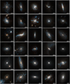 |
Fig. 2. Sample of mock images of galaxies at three different redshifts (z = 1.50, 1.15, and 0.80) is shown. The SDSS g-, r-, and i-band fluxes (mapped to blue, green, and red, respectively) are used to construct the color images. Based on stellar population and dust information, NEWCLUSTER successfully reproduces a wide variety of galaxy types. |
3.2. Galaxy scaling relations
In Fig. 3, we present some key scaling relations of galaxies from the NEWCLUSTER simulation at four different redshifts, z = 0.8, 1.5, 2.5, and 4.0. Each panel shows different galaxy properties on the y-axis as a function of their stellar mass on the x-axis. The black lines indicate empirical relations from observations, while the background pixels show the distribution of NEWCLUSTER galaxies at z = 0.8. The circles indicate median values of NEWCLUSTER galaxies at each snapshot, the standard error of the mean is shown as vertical lines only for z = 0.8 snapshot. Panel (a) shows the SFR versus stellar mass relation in comparison with observed main sequence from Whitaker et al. (2014). The distribution of galaxies at z ∼ 0.8 from Laigle et al. (2016) is also shown with 1σ and 2σ distributions as solid and dotted contours, respectively. SFR is measured based on the stars that are recognized as members of each galaxy. An overall decrease in the SFR sequence of NEWCLUSTER galaxies is observed with decreasing redshift. The sequence at z = 0.8 shows SFR lower than the empirical relation. This could be attributed to the fact that the zoom-in region lies in a highly over dense environment, where galaxies form earlier, and environmental quenching becomes effective. As a result, the galaxy population is significantly older than that of the average field.
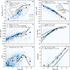 |
Fig. 3. Scaling relations of NEWCLUSTER galaxies measured at z = 0.8, 1.5, 2.5, and 4.0. The x-axis shows the stellar mass, and the y-axis in each panel indicates different scaling properties for galaxies. The pixels on the background represent the distribution of NEWCLUSTER galaxies at z = 0.8. Panel (a) presents the star formation rate of galaxies, which shows an overall decrease with redshift. Panel (b) presents the cold gas fraction of galaxies, which shows no strong evolution with redshift. However, the embedded figure in the panel, which presents the fraction of cold gas-deficient galaxies, shows an increase with redshift, particularly among lower-mass galaxies. Panel (c) presents half mass radius, which shows an increase over time over the entire mass range. Significant size growth is observed in high-mass galaxies, driven by mergers followed by wet compaction events. Panel (d) presents stellar metallicity, which exhibits a tight relation consistent with the empirical trend and shows no strong evolution with redshift. Panel (e) presents rotation velocity over velocity dispersion. Massive galaxies initially preferentially develop a strong rotation-supported system, which can be considered as disc settling, but experience a significant decrease in their rotation speed over time, indicating the formation of a slow rotator population through mergers. Panel (f) presents the mass of the most massive black holes in galaxies. The scaling relation lies well between the empirical relation of broad-line AGNs (solid line) and elliptical galaxies (dashed line). |
Panel (b) shows the fraction of cold gas in galaxies as a function of stellar mass. The cold gas mass is measured by summing the gas mass of cells with temperatures below 104 K within a radius of 2 R50, 3D from the galactic centre. Each median curve for the simulated galaxies has been measured for galaxies containing cold gas. The observational relations are from Catinella et al. (2018) and Zhang et al. (2021), where the former measured both atomic and molecular hydrogen at z = 0, while the latter measured only atomic hydrogen gas at z = 0.8. The gas mass of NEWCLUSTER galaxies does not change significantly with redshift, which is consistent with the result of Dubois et al. (2021). However, we find that the fraction of galaxies without any cold gas changes significantly with redshift, as shown in the embedded figure in the panel. This indicates that gas removal occurs in certain galaxies through the violent depletion of cold gas, likely driven by environmental effects.
Panel (c) shows galaxy sizes, represented by the half mass radius in 2-dimension, r50, 2D. To obtain a uniform distribution of lines of sight, we used 100 directions generated from Fibonacci lattices to measure apparent radii and used the median value of the distribution. Empirical relations are shown from Mowla et al. (2019), which includes all galaxy types (solid line), and from Nedkova et al. (2021), which separates galaxies into quiescent (dashed line) and star-forming (dotted line) types. The sizes of NEWCLUSTER galaxies show a moderate increase over time for lower-mass galaxies. The decrease in size-mass relation at high-redshift could be attributed to the gas-rich compaction event that takes place on galaxies above ∼1010 M⊙ (Dekel & Burkert 2014; Zolotov et al. 2015; Lapiner et al. 2021). These high-mass galaxies later show strong redshift evolution toward larger radii, likely driven by mergers (van der Wel et al. 2014). At z = 0.8, the empirical relation of star-forming galaxies closely overlaps with the lower-mass sequence of the simulated galaxies in the range of 108–1010 M⊙. The consistency seems to degrade at higher masses, while a plateau appears in the high-mass end of 1010 − 1011 M⊙. This can also be interpreted as the population transition from extended star-forming galaxies to compact, quiescent galaxies with increasing mass, where quenching is induced by the combination of mass and environmental effects within the cluster. Simulated galaxies more massive than 1011 M⊙ show smaller sizes compared to the empirical relation. This discrepancy is mainly due to their overly compact central stellar concentrations, which significantly reduce their half-mass radii, even though the most massive galaxies in the simulation clearly extend well beyond ∼ 10 kpc in radius.
Panel (d) presents the stellar mass versus stellar metallicity relation of NEWCLUSTER galaxies, measured in terms of [O/H], in comparison with empirical relations from Savaglio et al. (2005) and Wuyts et al. (2014). The NEWCLUSTER galaxies show no strong indication of evolution in the mass–metallicity relation across redshift. At z = 0.8, simulated galaxies show a tight relation that is consistent with observations, representing the continuous enrichment and recycling of gas within galaxies along with star formation. A minor population of galaxies appears in the upper-left region of the main sequence. Most of them turn out to be satellite galaxies that have undergone severe stripping, resulting in stellar mass loss that causes them to deviate from the main relation.
Panel (e) shows the stellar rotational velocity V divided by the velocity dispersion σ within galaxies. NEWCLUSTER galaxies exhibit a pronounced evolution in the relation across redshift. At high redshifts (z = 2.5 and 4.0), galaxies show stronger rotation at higher masses, consistent with a disc settling scenario that preferentially occurs in massive galaxies (Park et al. 2019). At low redshifts (z = 0.8 and 1.5), the most massive galaxies evolve into less rotationally supported systems, consistent with the formation of massive slow rotators through continuous mergers (Gerhard 1981; Barnes 1988; Choi & Yi 2017). This behavior is consistent with Dubois et al. (2016), who found that the (V/σ)* trend peaks around a stellar mass of 1011 M⊙. The median relation derived from the observed sample of Falcón-Barroso et al. (2019) at z ∼ 0 is shown as a black dashed line, which follows a similar trend to the extrapolated redshift evolution of the simulated galaxies toward lower redshift.
Panel (f) shows the mass of the most massive black holes within each galaxy, compared with the empirical relations of Suh et al. (2020) and Reines & Volonteri (2015). The former is derived from observations of broad-line AGNs at z < 2.5, shown as the solid line, while the latter is derived from classical bulges and ellipticals, shown as the dashed line. Regardless of the redshift, NEWCLUSTER galaxies lie between the elliptical and AGN relations and exhibit a large scatter around the empirical trends, reflecting the morphological diversity of the sample as seen in Fig. 2. NEWCLUSTER galaxies show a moderate increase in MBH mass at fixed stellar mass with decreasing redshift, suggesting a possible redshift evolution in the black hole mass–host galaxy mass relation. However, this trend may also be influenced by biases arising from the general morphological evolution of galaxies, as early-type galaxies become increasingly common at lower redshifts.
Figure 4 shows the stellar-to-halo mass ratio as a function of halo mass for NEWCLUSTER galaxies. The halo mass is measured at the peak mass of the main progenitor. Circles indicate the median of the distribution in each bin, color-coded with different redshifts. The 1σ scatter at z = 0.8 is shown as shades. Stars indicate individual galaxies with halo mass above 1013 M⊙. Empirical relations are shown for Behroozi et al. (2013a) as the solid line and Moster et al. (2010) as the dashed line. Although NEWCLUSTER galaxies lie in a high-density environment that may exhibit a stellar-to-halo mass ratio different from the universal relation, the excess of stellar mass in the intermediate-mass halos (Mhalo ∼ 1011 M⊙) may indicate the over production of stars for dwarf galaxies. This suggests that the current stellar feedback processes are not effective at suppressing star formation in low-mass galaxies at high redshifts. However, their effects at z < 1 appear to lead to an overly quenched population of galaxies, as shown in Panel (a) of Fig. 3.
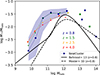 |
Fig. 4. Stellar-to-halo mass ratio as a function of halo mass for all central galaxies. Circles show median values in each bin, color-coded with different redshifts. Shade indicates 1σ scatter of the distribution at z = 0.8. Stars indicate individual galaxies. Empirical relations at z = 0.8 are shown as black lines. |
We present the photometric properties of NEWCLUSTER galaxies at z = 0.8 in Figure 5. The sample galaxies are the same as those in Fig. 3, but excluding misidentified clump-like substructures. We measure the g- and r-band absolute magnitudes using stellar age and metallicity, based on the simple stellar population models from Bruzual & Charlot (private communication)5. The top panel shows the g − r color versus r-band absolute magnitude, while the bottom panel presents the g-band surface brightness within the effective radius. Different colors indicate the r-band-weighted age of galaxies.
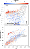 |
Fig. 5. Photometric properties of NEWCLUSTER galaxies at z = 0.8. The x-axis shows the r-band absolute magnitude. The y-axis of the top (bottom) panel represents g − r color (g-band effective surface brightness). We also present the black arrow to show the effect of dust attenuation assuming E(B − V) = 0.1 with Calzetti attenuation curve (Calzetti et al. 2000). The color of data points indicates the mass-weighted age of galaxies. The grey contours in both panels represent local observations from SDSS (Nair & Abraham 2010). |
The observed distributions of local galaxies are also displayed (Nair & Abraham 2010). Although the overall and median (green error bar) locations are not identical to observations, the trends are consistent with naive expectations. For instance, our color-magnitude distribution shows the separation between old and young populations, while the red sequence is not clearly separated at this redshift.
In the bottom panel, central surface brightness also linearly correlates well with absolute magnitude, as reported in observations of the Local Group (McConnachie 2012). We note that a separate cluster of objects is observed in the upper left of the main sequence. Their old age, low luminosity, and high surface brightness indicate that these objects are compact and quenched. After tracing their evolution through the merger tree, we find that they are not transient structures, as they show long, continuous histories without breaks. Since their progenitors are usually found as substructures within larger galaxies in terms of spatial distribution, they are likely ultra-compact dwarf galaxies (UCD) or orphan stellar systems that were ejected from larger galaxies (e.g., Jang et al. 2024). We leave the detailed investigation of these galaxies to future work.
Figure 6 shows the distribution of the stellar alpha enhancement fraction ([Mg/Fe]) as a function of metallicity ([Fe/H]). The grey background indicates the entire population of stars in the simulation, while the two contours show the members of galaxies in two different stellar mass ranges. As reported by previous studies (e.g., Bensby et al. 2014), the alpha-element enhancement fraction decreases with increasing metallicity, reflecting the differential enrichment from SNII and SNIa with their respective delay-time distributions. Comparing different stellar mass ranges, the stellar populations in more massive galaxies show overall higher metallicities and, at a given metallicity, higher alpha-element enhancement fractions. This indicates that the more massive galaxies in our simulation had more recycling of gas but with a shorter star formation history.
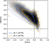 |
Fig. 6. Distribution of stars on the [Fe/H] – [Mg/Fe] chemical composition plane for galaxies in NEWCLUSTER at z = 0.8. The grey 2D histogram in the background indicates the distribution of all stars. Contours indicate stars which are members of galaxies with different stellar masses drawn by contours that contain 68.2% (solid lines) and 95.5% (dashed lines) of their distribution. |
3.3. Low-surface brightness structures
Low-surface brightness (LSB) structures, such as tidal streams, UDGs, and ICL, are emerging as key tracers of dynamical evolution through the assembly history (van Dokkum et al. 2015; Martin et al. 2019; Contini 2021; Contini et al. 2023). They are observed on a wide range of scales, from dwarf galaxies to massive galaxy clusters, and are generally defined as regions fainter than a surface brightness threshold of 22−24 mag arcsec−2 (Bothun et al. 1997; Bakos & Trujillo 2012; Tanoglidis et al. 2021). Thanks to the fine stellar mass resolution of our simulation, we are able to resolve these faint structures at z ∼ 0.8. LSB features of galaxies are receiving increasing attention due to their potential to shed light on the past assembly history of galaxies. UDGs are also interesting targets for studying extreme sites of star formation and their distinct characteristics compared to typical dwarf galaxies (van Dokkum et al. 2015; Pandya et al. 2018; Kado-Fong et al. 2022). Moreover, ICL has the potential to serve as an observable tracer of a cluster’s dynamical evolution and even the distribution of DM (Montes & Trujillo 2019; Contini 2021; Contini et al. 2023).
Despite being a broadly appealing target for study, LSB structures are inherently difficult to investigate due to their low detectability (Contini 2021; Yi et al. 2022; Joo & Jee 2023; Kelvin et al. 2023; Kim et al. 2023a). This is especially true at high redshifts, where galaxies may exhibit more dramatic tidal features because they are dynamically younger (Hopkins et al. 2010; Deger et al. 2018; Ferreira et al. 2020), but most studies are based on observations at z < 1 due to detection limits reduced by cosmological dimming. The emergence of cutting-edge instruments (e.g., JWST, LSST) presents an opportunity to extend our studies to higher redshifts and is expected to bring numerous LSB detections. It is necessary to prepare corresponding high-resolution simulations to resolve faint structures in a cosmological context in order to capture a wide range of their formation scenarios.
The minimum stellar particle mass of NEWCLUSTER is ∼2 × 10⁴ M⊙, which corresponds to a theoretical r-band surface brightness limit of 33.5 mag arcsec−2 at z = 0.8. This allows us to resolve faint structures on various scales. In the top panels of Fig. 7, we display stellar density maps of the ICL, a tidally distorted galaxy, and an LSB galaxy from left to right. Many faint structures are visible, not only in the ICL, but also in the trails of satellite galaxies. As more dynamical interactions are expected among galaxies in cluster environments (Dressler 1980; Jaffé et al. 2011; Yi et al. 2013), our simulation is well suited for studying the evolution of interacting galaxies down to the dwarf galaxy regime.
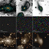 |
Fig. 7. Stellar density maps (top), mock SDSS, and JWST composite images (middle and bottom) of various objects in NEWCLUSTER. From left to right, images display the brightest cluster galaxy, tidal feature, and low-surface brightness galaxy samples. The sources from earlier snapshots are included to express the high-z background objects, and we also consider the k-correction to generate mock observations. Mock SDSS and JWST images are a composite of r, i, and z filters to cover the JWST range. We arbitrarily add a sky noise corresponding to 24 and 31 mag arcsec−1 for SDSS and JWST, respectively. The point spread functions are convolved with the pixelized source images. |
To enable direct comparison between our model and high-redshift observations, we also generate mock SDSS- and JWST-like images for these targets, shown in the middle and bottom panels of Fig. 76. We note that the mock SDSS images do not include the atmospheric seeing effect and therefore represent an idealized case compared to actual SDSS observations. It is challenging to capture the LSB features at z ∼ 0.8 with SDSS-like instruments (middle row). In particular, LSB galaxy is not visible in the SDSS mock image due to limited resolution and sensitivity, even though we select a relatively massive (M* = 3.5 × 10⁹ M⊙) galaxy. In contrast, applying the resolution and PSF of JWST (bottom row) enables the detection of faint structures seen in the stellar density map (top row).
A detailed investigation of the origins of the LSB features presented here is beyond the scope of this work. However, our results demonstrate that the simulation is well suited for direct comparison with high-redshift observational studies of LSB structures, including analyses of their detailed properties and evolutionary histories. The dense output cadence of ∼15 Myr allows us to trace the detailed motions of individual stellar particles stripped from galaxies. Moreover, by tracking both chemical and dust evolution, the model enables direct comparison with spectroscopic observations. Our simulation has not yet reached low redshifts, where LSB observational data are more abundant. Nevertheless, the current snapshot remains valuable not only for direct comparison with observations at z ∼ 0.8 but also for investigating the dynamical evolution of stars across a wide range of spatial scales.
3.4. Gas duty cycles and AGN feedback
Gas motion is intrinsically complex, governed not only by secular hydrodynamics but also by energetic astrophysical events such as SN explosions and AGN outflows. NEWCLUSTER is performed via AMR technique, an Eulerian approach that excels at capturing shocks and discontinuities during the feedback processes (Teyssier 2002; O’Shea et al. 2005; Hubber et al. 2013). However, despite this strength, AMR does not track the motion of individual gas cells, limiting its ability to follow Lagrangian gas trajectories, which is important for understanding the impact of feedback processes (Bellovary et al. 2013; Choi et al. 2024). In galaxy evolution studies, this makes it difficult to distinguish between inflowing and outflowing gas, which is crucial for understanding the cold gas supply and the impact of feedback on star formation.
To overcome this limitation, we applied Monte Carlo tracer particles that follow the hydrodynamics of gas cells (Genel et al. 2013; Cadiou et al. 2019). Cadiou et al. (2019) demonstrated that Monte-Carlo tracers exhibit better performance than velocity-advected models in tracing the gas motion and spatial distribution in cosmological simulations. The simulation includes 267 997 944 tracer particles in total. These tracer particles probabilistically move between cells and stars, and massive black hole particles based on their gas mass exchange events, such as flux between cells, star formation, mass ejection from feedback, and accretion. Tracer particles provide valuable opportunities by allowing the tracking of actual gas motions via particle IDs within the simulation framework. We found that the spatial distribution of gas tracers closely resembles the density distribution of gas cells within the simulation. However, we note that the discrete number of tracer particles cannot perfectly reproduce the true transport of gas mass, a limitation shared with the full Lagrangian approach.
In Fig. 8, we show the trajectories of gas tracer particles within a galaxy as an example of their use in tracking gas dynamics. The central galaxy (M* = 2.2 × 10¹² M⊙ in Mhost = 4.63 × 10¹³ M⊙) experiences a violent AGN outburst at z = 1.6. We first selected sample gas tracers that were initially located within R90, 3D of the central galaxy and further classified them into three categories based on their trajectories before and after 500 Myr:
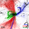 |
Fig. 8. Smoothed trajectories of gas tracer particles that are located in the central region of the galaxy at z = 1.6. The greyscale background represents the gas temperature (i.e., cold gas in a darker color). Blue lines are the trajectory of the inflow gas 500 Myr before the central AGN activity. Red lines indicate outflow gas expelled by the violent jet. Green lines are similarly blown out but return back to the galactic disc. |
-
Inflow: the time when the tracer is farthest from the central MBH occurs before reaching its pericentre, and its maximum distance exceeds 10 R90, 3D.
-
Outflow: the tracer reaches a maximum distance greater than 6 R90, 3D and continues to move away from the centre for at least 400 Myr.
-
Recycle: the tracer travels outward beyond 2.5 R90, 3D but later returns within 1.5 R90, 3D.
We show the smoothed trajectories of individual gas tracer particles, classified into each category and color-coded accordingly. The background displays the gas temperature. Since the target galaxy is moving from left to right, most of the inflowing gas (blue) originates from the right side of the figure. However, it is clearly visible that some gas inflow also originates from the bottom, exhibiting a narrowly-channeled feature that indicates gas brought in by an infalling satellite galaxy. We note that the theoretical study reported that the most stream influx comes from one or few dominant streams (Danovich et al. 2012). Outflowing tracers (red) rapidly escape from the galactic centre along the bipolar AGN jet axis, which is aligned with the galaxy’s rotation axis. They also show highly turbulent motion after reaching the low-density circumgalactic region. Recycled tracers (green) do not display a strongly preferential direction, in contrast to inflow or outflow tracers. The presence of recycled gas demonstrates that a significant amount of gas can escape from the galactic disc and later return, consistent with the galactic fountain scenario (Bregman 1980; Melioli et al. 2008).
Tracer particles are directly applicable to investigate how AGN feedback ejects galactic gas and regulates central star formation. Moreover, as our simulation is set in a cluster environment, it is also suited to studying how gas in satellite galaxies is stripped in ICM by ram pressure or how their gas supply is halted. Tracer particles also provide a means to study the MBH duty cycle (Martini & Weinberg 2001; Choi et al. 2024). Since we track the state transition of tracer particles to gas, star, and MBH tracers, we can distinguish the gas consumed by accretion from that expelled by feedback.
3.5. Ram-pressure stripping of gas
Cluster environments host the most significant gas removal processes observed in galaxies. The interaction between the hot ICM and the ISM of galaxies moving at velocities of ∼1000 km s−1 exerts strong pressure, estimated as Pram/kB ∼ 105 − 6 K cm−3 (Jung et al. 2018; Yun et al. 2019; Boselli et al. 2021), following the formulation of Gunn & Gott (1972). This external pressure often exceeds the internal gravitational restoring force of galaxies, leading to the stripping of their gas components. Observations of gas trails including jellyfish phenomenon (e.g., Kenney et al. 2004; Chung et al. 2009; Jaffé et al. 2018) provide evidence for this mechanism. The resulting gas loss effectively quenches star formation (SF), often on short timescales although a temporal enhancement of SF activity occurs due to compression of ISM (e.g., Crowl & Kenney 2006; Vulcani et al. 2018; Roberts & Parker 2020). Consequently, strong ram pressure, in combination with other environmental mechanisms, is now recognized as a driver of the high fraction of passive galaxies observed in clusters (e.g., Contini et al. 2020; Rhee et al. 2020; Oman et al. 2021).
An important next step is to understand how complex the interactions between the ICM and ISM truly are, and how gas is stripped from galaxies in a manner that reproduces the observed morphologies. One effective approach is the use of idealized wind-tunnel simulations, where a uniform ICM wind is applied to a model galaxy to mimic ram pressure stripping (e.g., Bekki 2009; Tonnesen & Bryan 2012; Lee et al. 2020; Choi et al. 2022). These simulations offer very high spatial and temporal resolution, enabling detailed studies of gas dynamics under controlled conditions. However, a key limitation is that the ram pressure strength is often assumed to be constant, which does not reflect the time-varying conditions experienced by galaxies in live halos (cf., Tonnesen 2019). Recent studies suggest that such variations in ram pressure may play a role in shaping both the gas content and morphology of galaxies (e.g., Samuel et al. 2023; Zhu et al. 2024). Therefore, it is essential to incorporate realistic ram pressure profiles when studying its effects on galaxies.
Cosmological hydrodynamic simulations provide a complementary framework for studying the impact of ram pressure on galaxy evolution. For example, Jung et al. (2018) used the YZiCS simulation (Choi & Yi 2017) to investigate gas removal in clusters, finding that strong ram pressure near cluster centres is a dominant driver of gas deficiency in satellite galaxies. Several other studies employing cosmological simulations (e.g., Lotz et al. 2019; Yun et al. 2019; Rohr et al. 2023) have similarly concluded that ram pressure plays a central role in driving environmental quenching in clusters. However, these cosmological simulations often lack the spatial resolution necessary to capture the complexity of ICM-ISM interactions, particularly the multiphase or clumpy nature of ISM, which may be more resilient to stripping. As a result, there is significant potential for overestimating or overlooking ram pressure effects in cosmological simulations, especially when small-scale physical processes fall below the resolution limit.
The NEWCLUSTER simulation bridges the gap between idealized and cosmological approaches to studying ram pressure stripping. Its spatial resolution is sufficient to capture high-density gas components–possibly corresponding to the molecular phase of ISM–that are expected to be less sensitive to ram pressure (e.g., Tonnesen & Bryan 2009). In addition, the mass resolution enables the modeling of ram pressure effects on dwarf galaxies with M* > 107 − 9 M⊙, which is a mass range that remains largely inaccessible to most large-scale simulations. Although NEWCLUSTER does not extend to the local Universe, it captures the high-redshift regime (z > 0.8), a period when ram pressure was already a significant environmental process (e.g., Simons et al. 2020). As such, the simulation offers an opportunity to investigate the early formation of gas-poor galaxies in dense environments and to shed light on the onset of environmental quenching in nascent clusters.
The upper panel of Fig. 9 illustrates the gas distributions within the main cluster in NEWCLUSTER at z = 1, where the gas column density is color-coded and the virial radius of the main cluster is shown as the grey circle. Although the cluster has not yet reached the canonical mass range for local clusters (Mvir > 1014 M⊙), numerous galaxies display extended gas tails, indicating that ram pressure effects are already active at z = 1. To evaluate whether ram pressure is sufficiently strong to influence galaxy evolution, we compute its value for individual galaxies surrounding clusters. The volume-weighted mean ram pressure is measured using ICM gas cells, following the methodology of the ICM gas selection in Rhee et al. (2024):
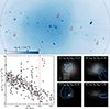 |
Fig. 9. Upper panel: Gas column density map of the main cluster in the NEWCLUSTER simulation at z = 1. The virial radius of the cluster is drawn with a grey circle. Numerous galaxies show gas tails within the early-stage cluster. Four galaxies chosen for representative illustration are marked with red circles. Bottom panel (left): Radial profile of the ram pressure exerted on galaxies (grey circles). The red dashed vertical line shows the virial radius. An evident decreasing trend of the magnitude of ram pressure can be seen. The ram pressures of the four representative galaxies are shown with the red circles. Bottom panel (right): Stellar density and gas column density distributions of the four galaxy samples. In each panel, the background density map is the surface brightness of the galaxy in r-band, and the contours show the column density distributions of cold gas. The red arrow indicates the direction of motion of the galaxy. |
 (5)
(5)
where ρi, vi, and Vi are the density, velocity with respect to the galaxy, and the volume of i-th gas ICM cell, respectively. The bottom left panel of Fig. 9 presents the radial profile of ram pressure across the galaxy sample. A clear decline in ram pressure with increasing distance is seen, primarily reflecting the decreasing ICM density at larger radii. The scatter in this trend is likely driven by variations in galaxy velocities. In addition, galaxy–galaxy interactions can also induce strong ram pressure. For example, galaxies experiencing strong ram pressure at around D3D = 250 or 450 kpc are satellites undergoing significant ram pressure from the gas disc of a massive galaxy. Notably, galaxies located near the cluster core experience ram pressure values on the order of Pram/kB ∼ 106 K cm−3, consistent with estimates for local clusters (Jung et al. 2018; Yun et al. 2019; Boselli et al. 2021).
The bottom-right panels of Fig. 9 display four typical galaxies with different stellar masses undergoing ram pressure stripping, each of which is also marked in the cluster gas density map with the red circles in the upper panel. In each panel, the background shows the stellar surface density, while overplotted contours trace the column density of cold gas, with different contour levels with different colors. The red arrow indicates the direction of motion of the galaxies. All four galaxies exhibit asymmetric gas morphologies, with cold gas displaced in the direction opposite to their motion–a characteristic signature of ram pressure stripping. Notably, Galaxy D, which has the lowest stellar mass and experiences the strongest ram pressure among the four, shows complete removal of its cold gas, illustrating the dramatic impact of ram pressure stripping in low-mass galaxies.
Therefore, the NEWCLUSTER simulation is useful to study the impact of ram pressure in early clusters on satellite galaxies across a wide range of stellar mass. Comparing the measured strength of ram pressure with the restoring force inside galaxies provides quantitative investigation of the origin of gas stripping. Determining whether galaxies undergoing ram pressure retain their gas and continue SF, or are fully quenched, remains an important topic for future studies. The use of tracer particles also enables the study of the distribution of stripped gas inside cluster halos, but we defer such a detailed investigation to future work.
3.6. Dust properties
The JWST presents the unprecedented data of the early Universe. Understanding the data requires a proper knowledge of dust properties and of its evolution because dust changes the intrinsic spectral energy distribution (SED) of galaxies significantly.
Numerical simulations have recently begun to follow dust evolution in a cosmological context on the fly, including dust formation, destruction, and the evolution of chemical composition and grain size (Davé et al. 2019; Jones et al. 2024; Choban et al. 2025). This approach goes well beyond the simpler post-processing methods that map dust onto the metal mass content of the gas. Since NEWCLUSTER tracks the evolution of carbonaceous and silicate grains separately, it enables a detailed examination of the distinct behaviors of different dust species as they respond to dynamic environmental changes such as mergers, AGN feedback, and starbursts on short timescales. We also trace the evolution of grain size. Under the two-size approximation, small and large grains form and evolve through different but interrelated processes. By combining grain size and chemical composition information, we can investigate the evolution of the intrinsic dust extinction curve and generate realistic mock observations, even at high redshifts.
Figure 10 shows the dust properties of a sample spiral galaxy at z = 0.8. The left panel shows the intrinsic extinction curve based on the average composition of dust inside 3 R50, 3D using Mie theory and grain optical constants from Weingartner & Draine (2001). The total extinction curve is shown in grey, and the cyan and magenta lines represent the carbon-based and silicon-based grain species, respectively. The contributions from small and large grains are shown with different line styles (dotted and dashed lines for small and large grains, respectively), and the grain size distribution is also presented in a sub-panel in the upper right corner.
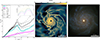 |
Fig. 10. Example galaxy extinction curve and corresponding mock observation. The extinction curve is shown in the first column of the figure. The total extinction curve (grey) is presented along with the contributions from graphite (cyan) and silicate (magenta) grains, each shown with two different size distributions (dotted lines for small grains and dashed lines for large grains). The MW (Fitzpatrick & Massa 2007) extinction, SMC (Pei 1992) extinction, and Calzetti attenuation curves are also included for comparison. The grain size distributions for different grain types are shown in the sub-panel, with the MRN (Mathis et al. 1977) slope indicated by a yellow dashed line. The spatial distribution of the DTM is shown in the second column. The corresponding mock image, created using SDSS g, r, and i bands for RGB, is shown in the last column. |
The Milky Way (MW) average extinction curve (Fitzpatrick & Massa 2007), the Small Magellanic Cloud (SMC) extinction curve (Pei 1992), and the Calzetti attenuation curve for starburst galaxies (Calzetti et al. 2000) are also given for reference. We note that, unlike the MW and SMC extinction curves, the Calzetti curve represents an attenuation law that encapsulates both absorption and scattering effects in a mixed star–dust geometry (for reference, see Narayanan et al. 2018, which illustrates how Calzetti-like attenuation laws can emerge from different extinction curves depending on the geometry between stars and dust). The sample NEWCLUSTER galaxy shows a UV-to-optical slope similar to the Calzetti attenuation curve, but notably with a clear 2175 Å bump as shown in the MW curve produced by small carbonaceous grains.
The spatial distribution of the dust-to-metal mass ratio (DTM) is also presented in the middle panel. The mean DTM inside 3 R50, 3D is ∼0.4. We find that the DTM of the dust lanes following the spiral arms (see the RGB composite mock image in the right panel, generated using SKIRT with the SDSS u-, g-, and r-bands mapped to blue, green, and red, respectively) is nearly 0.5 or above, but shows various values over a wide range. We notice a large cavity of DTM ratio in the centre and small ones in the spiral arms. They are the sites of enhanced star formation, where SN shocks destroy a large fraction of the dust. The central DTM cavity is of particular significance, because it seriously affects the apparent light distribution of galaxies and thus morphology determination at high redshifts (Byun et al. 2025).
3.7. Cluster merger
The main halo in the NEWCLUSTER simulation is approaching a major merger event (mass ratio 1:3.2). The second-largest halo lies in close proximity, with its first encounter expected at z ≈ 0.774 and final coalescence at z ≈ 0.35, according to the DM-only pilot simulation. Figure 11 illustrates a comprehensive, multicomponent view of the main and secondary halos involved in the major merger. The upper six panels display: (A) DM density, (B) stellar density, (C) gas column density, (D) gas temperature, (E) the Sunyaev-Zeldovich (SZ) signal computed using the Compton y-parameter, which traces the integrated pressure along the line of sight (Nelson et al. 2024), and (F) gas metallicity. The two halos are projected onto a plane containing the collision axis, providing a clear view of their relative structure and separation. Red and black dashed circles indicate the virial radii of the primary and secondary halos, respectively.
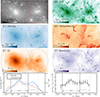 |
Fig. 11. Multicomponent view of the merging clusters at z = 0.73 with different components (six upper panels) and 1D profiles of the merging clusters (bottom two panels). From (A) to (E), DM surface density, stellar surface density, gas column density, temperature, the Sunyaev-Zeldovich signal by the y-parameter, and metallicity are shown, in which virial radii of the clusters are drawn with dashed circles. The compression of ICM caused by the major merger can be seen by a high contrast of y-parameter at the merger front. The bottom-left panel shows the 1D profiles of density (blue solid line) and temperature (red solid line) along the collision axis. The locations of the virial radii are shown with the vertical lines. The bottom-right panels display the median ram pressure profiles of galaxies along the collision axis. Galaxies at the merger boundary (0 kpc ≲ ΔX ≲ 300 kpc) undergo higher external pressure compared to those on the far side of the merger front. |
The bottom-left panel presents the one-dimensional (1D) profiles of gas density (blue solid line) and temperature (red solid line) measured along the collision axis. The virial radii of the main and companion clusters are marked by the dark grey solid line and the light grey dashed line, respectively. There is a noticeable increase in temperature and pressure near the interface, indicating that compressive heating is occurring in the ICM. This feature is also evident in the Panels D and E. In contrast, the gas metallicity in this region remains low, suggesting that the high-temperature gas is not a product of metal-enriched outflows from galaxies. This supports the interpretation that the outer ICM of both clusters is being compressed as a direct consequence of the ongoing cluster-cluster merger.
The bottom right panel of Fig. 11 shows the median ram pressure experienced by galaxies along the collision axis. Notably, galaxies located between the two clusters are subject to elevated ram pressure compared to galaxies at similar distances on the far side of the merger front. This enhancement is a consequence of the ICM compression, indicating that galaxies can be affected by cluster-cluster mergers, even though they are treated as collisionless components in large-scale dynamics. Such an increased ram pressure may lead to triggered SF or AGN activity in some galaxies (Owen et al. 1999; Miller & Owen 2003; Stroe et al. 2014; Stroe & Sobral 2021). In this context, NEWCLUSTER provides a valuable platform for investigating the impact of large-scale mergers on galaxy evolution.
3.8. Quenching of galaxies in Clusters
Red and dead galaxies preferentially reside in high-density environments in the local Universe (Dressler 1980; Lewis et al. 2002; Hogg et al. 2004; Kauffmann et al. 2004). In contrast, these regions likely experienced elevated star formation activity in the early Universe (Jeon et al. 2022). Observations suggest that substantial environmental quenching was already underway at high redshifts. For example, Gerke et al. (2007) reported an excess of blue galaxies in low-density regions (groups and the field) at z ≲ 1. Furthermore, the emergence of a well-defined color-magnitude relation in galaxy clusters at z ∼ 1 (Ellis et al. 1997; Kodama et al. 1998; Stanford et al. 1998; Mei et al. 2006a,b) supports the idea of early galaxy formation in dense environments. The presence of a red sequence on the color-magnitude plane at these redshifts is considered a hallmark of such accelerated evolution. Evidence of rapid environmental influence extends to even higher redshifts (e.g., z > 2; Steidel et al. 2005), and JWST observations have begun tracing the formation and evolution of galaxies in overdense regions beyond z ∼ 5 (e.g., Alberts et al. 2024; Morishita et al. 2025). These findings suggest that environmental effects may have already played a significant role in shaping galaxy populations at z > 1.
In this context, NEWCLUSTER is particularly well suited for investigating the origin of SF quenching at high redshifts, as it extends beyond z = 1 and contains several thousand satellite galaxies residing in high-density environments. For example, we select two halos with Mvir > 1013 M⊙ at z = 1. Galaxies with M* > 109 M⊙ located within three virial radii of these halos are selected and classified based on their SF activity. Specifically, galaxies are divided into star-forming (b > 0.1) or quenched (b < 0.1) populations, where b = tUniverse × SFR/M* is the birth rate parameter widely used to quantify the degree of SF quenching across a broad range of redshift and stellar masses, with tUnivserse denoting the age of the Universe (Franx et al. 2008; Lotz et al. 2019; Park et al. 2022; Rhee et al. 2024). The SFR is measured over a 100 Myr timescale. At this stage, galaxies with M* < 109 M⊙ are excluded from the classification, as the majority of these low-mass galaxies exhibit negligible or no SF activity. Their rapid quenching is likely driven by their shallow gravitational potentials, which make them highly susceptible to environmental processes within clusters.
Figure 12 presents the phase-space distribution of the galaxies, with all galaxies shown in grey, and quenched and star-forming populations in red and blue, respectively. Positions and velocities are normalized by the virial radius and velocity dispersion of the host clusters. The black dashed curve denotes the escape velocity profile of the most massive halo, providing a reference for the dynamical boundaries of the clusters. To illustrate the spatial concentration of each population, 0.5σ and 1σ contours are overlaid for quenched (red lines) and star-forming galaxies (blue lines).
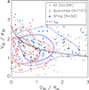 |
Fig. 12. Phase space diagram of galaxies in two dark matter halos with Mvir > 1013 M⊙ at z = 1. The black dashed line is the escape velocity curve profile of the more massive halos. Galaxies with M* > 109 M⊙ are classified into two groups, either they are star-forming (b > 0.1) or quenched (b < 0.1). See the texts for the definition of the parameter b. Their 0.5σ and 1σ distributions are displayed with the contours with dashed line and solid line, respectively. Even at a high redshift of z = 1, a clear separation between the distributions of star-forming and quenched galaxies is seen. |
The quenched galaxies (red circles) are primarily concentrated within the virial radius, whereas star-forming galaxies tend to occupy the outer regions, consistent with them being a recently-accreted population (Rhee et al. 2017). This clear separation between the two distributions suggests a scenario in which galaxies are rapidly quenched following infall into their host clusters. A similar separation between quenched and star-forming populations has been observed in clusters at the local Universe, where phase-space diagrams reveal strong correlations between the quenching status and the orbital history of galaxies (e.g., Oman & Hudson 2016; Rhee et al. 2020; Oman et al. 2021). These findings highlight the predictive power of phase-space analysis that extends beyond the local universe and remains effective even at high redshifts (e.g., Muzzin et al. 2014; Kim et al. 2023b).
Given that the environmental effects in the clusters are already evident by z = 1 (e.g., Gay et al. 2010), the NEWCLUSTER simulation is well positioned to support a range of follow-up studies. One important direction is to investigate the physical mechanisms driving rapid quenching, which likely account for the lack of star-forming galaxies in cluster core regions. Beyond the impact on newly-accreted satellites, the simulation also offers an opportunity to examine the evolution of the Butcher-Oemler effect (Butcher & Oemler 1978) at high redshifts, providing insights into the pace of galaxy transformation in high-density environments. Such studies will be particularly valuable when interpreted alongside recent JWST observations tracing early galaxy populations in overdense regions.
4. Summary
This paper introduces the current status of the NEWCLUSTER simulation and outlines potential scientific investigations it enables. The functioning of the simulation is as follows: a cluster region is selected from a cosmological volume with a side-length of 100 h−1 Mpc, and is subsequently re-simulated at high resolutions, incorporating a comprehensive and modern astrophysics model (see Sect. 2). In addition to the standard prescriptions for SF and feedback models from stars and super-massive black holes (SMBHs), NEWCLUSTER performs on-the-fly modeling of dust evolution and chemical enrichment for ten species (H, D, He, C, N, O, Mg, Fe, Si, and S). These capabilities allow for the investigation of previously inaccessible aspects of galaxy evolution in a cosmological context. For instance, the processes involved in shaping galaxy morphologies at high redshifts, informed by dust extinction from realistic dust distributions within galaxies, has been studied in Byun et al. (2025). Figure 2 highlights these novel features, presenting mock images of NEWCLUSTER galaxies that closely resemble real observations.
Since the simulation aims to reproduce one of the most complex regions of the universe at very high resolution, NEWCLUSTER requires computationally intensive calculations. For example, the simulation reached z = 0.8, taking more than 108 CPU hours. These extensive calculations have been made possible thanks to significant scalability enhancements in the RAMSES code, achieved through hybrid parallelization with OpenMP and MPI (Han et al. 2025). The updated RAMSES code shows efficient performance in using numerous CPU cores simultaneously, with which the NEWCLUSTER simulation is running using 7680–15 360 threads, depending on the speed and resource situations.
By achieving high resolution (e.g., 68 pc for spatial resolution) in a cluster simulation, NEWCLUSTER enables detailed studies of galaxy evolution across a wide mass range within cosmological cluster environments. As a result, several key scientific investigations become feasible. The excellent stellar mass resolution of NEWCLUSTER (∼2 × 10⁴ M⊙) allows for the detection of LSB features down to μ ∼ 33.5 mag arcsec−2 at z ∼ 0.8. Importantly, the cluster environment targeted by NEWCLUSTER is particularly rich in LSB structures, including tidal debris, UDGs, and ICL. Figure 7 showcases a variety of such LSB features captured in the simulation.
One of the key features of NEWCLUSTER is an embedding of the Monte Carlo tracer particle to track the Lagrangian motion of gas cells. With the successful capture of the small-scale galactic features via recent hydrodynamical simulations, we went on to investigate the detailed trajectory and evolutionary pathway of gas to building those features. The tracer particles in NEWCLUSTER recover the true distribution of gas. Figure 8 shows an example of the prospect of tracer particles. NEWCLUSTER with tracer particles would extend our interests to various topics, such as gas recycling in star formation or MBH accretion, distinguishing the inflow and outflow gases.
Although NEWCLUSTER does not yet extend to the Local Universe, it reaches the formation epoch of the cluster and provides critical insights into the evolution of galaxies in the first half of the history of the Universe. As shown in Fig. 9, ram pressure is already affecting satellite galaxies at this epoch, with many displaying jellyfish-like morphologies. Galaxy D in Fig. 9, for example, exhibits complete gas removal. These early interactions contribute to the emergence of gas-deficient galaxies well before the present day. Moreover, likely due in part to the effects of ram pressure, Figure 12 reveals a clear separation between star-forming and quenched galaxies in the early clusters in the phase space, suggesting that environmental quenching is already effective at z ∼ 1. The presence of passive galaxies in such early structures raises important questions about the onset and efficiency of environmental effects in the high-redshift Universe.
Advancing toward a better understanding of dust evolution through cosmic time might be one of the most important and urgent tasks in the JWST era. Because not only the chemical composition of grain species but also their geometric distribution matters, a physically motivated theoretical prediction in a cosmological context is crucial. Although many cosmological simulations have included dust evolution on-the-fly (Gjergo et al. 2018; Hou et al. 2019; Trebitsch et al. 2021; Granato et al. 2021; Lewis et al. 2023), NEWCLUSTER is one of the pioneering cosmological simulations to simultaneously track both the grain size distribution and chemical composition of dust down to redshifts z < 1.
Figure 10 clearly shows how calculations with different grain species (carbon- and silicon-based) and different size bins successfully reproduce the extinction curve. Despite the fact that our dust model is built on a relatively simple prescription compared to the real universe, we hope that our results can serve as a cornerstone for a better understanding of dust evolution from the high-redshift universe to the local universe. NEWCLUSTER represents a first step toward that goal.
NEWCLUSTER at z ∼ 0.8 captures a notable pre-merger configuration, in which the main cluster and the second most massive halo are approaching one another. Figure 11 illustrates a multidimensional view of the two halos at this early merger stage. At the interface between the halos, signatures of gas compression are evident, particularly at the merger front, wherein galaxies are subject to enhanced ram pressure. These conditions suggest that cluster-cluster mergers can significantly influence galaxy evolution, even prior to the core passage. The results highlight the possibility that such mergers may trigger SF in some galaxies while accelerating quenching in others. NEWCLUSTER thus offers a powerful platform for studying how large-scale dynamical events reshape galaxy populations during the assembly of massive structures. NEWCLUSTER will soon reveal the complete merger between the clusters at around z ≈ 0.5. This will allow a number of exciting investigations on galaxy evolution as well as cluster evolution.
The NEWCLUSTER simulation enables a broad range of follow-up studies, spanning scales from SMBH to the cosmic web. A list of ongoing science cases is available on the simulation website7. To support and encourage further research, we have provided public access to the NEWCLUSTER dataset via the website, including the galaxy and halo catalog, subset of raw simulation outputs, and mock images. We welcome participation from the community in expanding the scientific exploration enabled by this simulation.
A critical shortcoming of NEWCLUSTER is that it is only one cluster and, thus, it cannot be broadly representative. However, it is already a considerable challenging to obtain results for a single cluster done at such resolutions. After three years of nearly continuous runs, we only reached z = 0.88 and we expect to require a similar or greater amount of computing time to reach the Local Universe. Now that we see the beauty and power of high-resolution data, we want to continue the march toward simulating more clusters. In striving to achieve this goal, a dramatically improved numerical approach would be necessary.
Acknowledgments
S.K.Y. acknowledges support from the Korean National Research Foundation (RS-2025-00514475 and RS-2022-NR070872). This work was granted access to the HPC resources of KISTI under the allocations KSC-2021-CRE-0486, KSC-2022-CRE-0088, KSC-2022-CRE-0344, KSC-2022-CRE-0409, KSC-2023-CRE-0343, KSC-2024-CHA-0009, and KSC-2025-CRE-0031 and of GENCI under the allocation A0150414625 and A0180416216. The large data transfer was supported by KREONET which is managed and operated by KISTI. J.R was supported by the KASI-Yonsei Postdoctoral Fellowship and was supported by the Korea Astronomy and Space Science Institute under the R&D programme (Project No. 2025-1-831-02), supervised by the Korea AeroSpace Administration. This work was partially supported by the Institut de Physique des deux infinis of Sorbonne Université and by the ANR grant ANR-19-CE31-0017 of the French Agence Nationale de la Recherche. J.K. is supported by KIAS Individual Grants (KG039603) at the Korea Institute for Advanced Study. T.K. is supported by the National Research Foundation of Korea (RS-2025-00516961) and the Yonsei Fellowship funded by Lee Youn Jae.
References
- Alberts, S., Williams, C. C., Helton, J. M., et al. 2024, ApJ, 975, 85 [Google Scholar]
- Aoyama, S., Hou, K.-C., Shimizu, I., et al. 2017, MNRAS, 466, 105 [NASA ADS] [CrossRef] [Google Scholar]
- Aubert, D., Pichon, C., & Colombi, S. 2004, MNRAS, 352, 376 [Google Scholar]
- Bahé, Y. M., Schaye, J., Schaller, M., et al. 2022, MNRAS, 516, 167 [CrossRef] [Google Scholar]
- Bakos, J., & Trujillo, I. 2012, ArXiv e-prints [arXiv:1204.3082] [Google Scholar]
- Barnes, J. E. 1988, ApJ, 331, 699 [NASA ADS] [CrossRef] [Google Scholar]
- Barnes, D. J., Kay, S. T., Bahé, Y. M., et al. 2017, MNRAS, 471, 1088 [Google Scholar]
- Behroozi, P. S., Wechsler, R. H., & Conroy, C. 2013a, ApJ, 770, 57 [NASA ADS] [CrossRef] [Google Scholar]
- Behroozi, P. S., Wechsler, R. H., & Wu, H.-Y. 2013b, ApJ, 762, 109 [NASA ADS] [CrossRef] [Google Scholar]
- Bekki, K. 2009, MNRAS, 399, 2221 [Google Scholar]
- Bellovary, J., Brooks, A., Volonteri, M., et al. 2013, ApJ, 779, 136 [Google Scholar]
- Bensby, T., Feltzing, S., & Oey, M. S. 2014, A&A, 562, A71 [NASA ADS] [CrossRef] [EDP Sciences] [Google Scholar]
- Biernacki, P., Teyssier, R., & Bleuler, A. 2017, MNRAS, 469, 295 [Google Scholar]
- Boselli, A., Lupi, A., Epinat, B., et al. 2021, A&A, 646, A139 [NASA ADS] [CrossRef] [EDP Sciences] [Google Scholar]
- Bothun, G., Impey, C., & McGaugh, S. 1997, PASP, 109, 745 [NASA ADS] [CrossRef] [Google Scholar]
- Bower, R. G., Benson, A. J., Malbon, R., et al. 2006, MNRAS, 370, 645 [Google Scholar]
- Bregman, J. N. 1980, ApJ, 236, 577 [NASA ADS] [CrossRef] [Google Scholar]
- Bryan, G. L., & Norman, M. L. 1998, ApJ, 495, 80 [NASA ADS] [CrossRef] [Google Scholar]
- Butcher, H., & Oemler, A., Jr. 1978, ApJ, 219, 18 [NASA ADS] [CrossRef] [Google Scholar]
- Byun, G.-H., Jang, J. K., Scofield, Z. P., et al. 2025, ApJ, 992, 92 [Google Scholar]
- Cadiou, C., Dubois, Y., & Pichon, C. 2019, A&A, 621, A96 [NASA ADS] [CrossRef] [EDP Sciences] [Google Scholar]
- Calzetti, D., Armus, L., Bohlin, R. C., et al. 2000, ApJ, 533, 682 [NASA ADS] [CrossRef] [Google Scholar]
- Carniani, S., Hainline, K., D’Eugenio, F., et al. 2024, Nature, 633, 318 [CrossRef] [Google Scholar]
- Catinella, B., Saintonge, A., Janowiecki, S., et al. 2018, MNRAS, 476, 875 [NASA ADS] [CrossRef] [Google Scholar]
- Chabrier, G. 2003, PASP, 115, 763 [Google Scholar]
- Chandrasekhar, S. 1943, ApJ, 97, 255 [Google Scholar]
- Choban, C. R., Salim, S., Kereš, D., Hayward, C. C., & Sandstrom, K. M. 2025, MNRAS, 537, 1518 [Google Scholar]
- Choi, H., & Yi, S. K. 2017, ApJ, 837, 68 [NASA ADS] [CrossRef] [Google Scholar]
- Choi, W., Kim, C.-G., & Chung, A. 2022, ApJ, 936, 133 [NASA ADS] [CrossRef] [Google Scholar]
- Choi, E., Somerville, R. S., Ostriker, J. P., Hirschmann, M., & Naab, T. 2024, ApJ, 964, 54 [CrossRef] [Google Scholar]
- Chokshi, A., Tielens, A. G. G. M., & Hollenbach, D. 1993, ApJ, 407, 806 [Google Scholar]
- Chung, A., van Gorkom, J. H., Kenney, J. D. P., Crowl, H., & Vollmer, B. 2009, AJ, 138, 1741 [Google Scholar]
- Cole, S. 1991, ApJ, 367, 45 [Google Scholar]
- Contini, E. 2021, Galaxies, 9, 60 [NASA ADS] [CrossRef] [Google Scholar]
- Contini, E., Gu, Q., Ge, X., et al. 2020, ApJ, 889, 156 [NASA ADS] [CrossRef] [Google Scholar]
- Contini, E., Jeon, S., Rhee, J., Han, S., & Yi, S. K. 2023, ApJ, 958, 72 [NASA ADS] [CrossRef] [Google Scholar]
- Crowl, H. H., & Kenney, J. D. P. 2006, ApJ, 649, L75 [CrossRef] [Google Scholar]
- Cuppen, H. M., & Herbst, E. 2007, ApJ, 668, 294 [Google Scholar]
- Cyburt, R. H., Fields, B. D., Olive, K. A., & Yeh, T.-H. 2016, Rev. Mod. Phys., 88, 015004 [NASA ADS] [CrossRef] [Google Scholar]
- Dalgarno, A., & McCray, R. A. 1972, ARA&A, 10, 375 [Google Scholar]
- Danovich, M., Dekel, A., Hahn, O., & Teyssier, R. 2012, MNRAS, 422, 1732 [Google Scholar]
- Davé, R., Anglés-Alcázar, D., Narayanan, D., et al. 2019, MNRAS, 486, 2827 [Google Scholar]
- Davis, M., Efstathiou, G., Frenk, C. S., & White, S. D. M. 1985, ApJ, 292, 371 [Google Scholar]
- De Lucia, G., & Blaizot, J. 2007, MNRAS, 375, 2 [Google Scholar]
- Deger, S., Rudnick, G., Kelkar, K., et al. 2018, ApJ, 869, 6 [Google Scholar]
- Dekel, A., & Burkert, A. 2014, MNRAS, 438, 1870 [Google Scholar]
- Dressler, A. 1980, ApJ, 236, 351 [Google Scholar]
- Du, M., Ho, L. C., Debattista, V. P., et al. 2021, ApJ, 919, 135 [NASA ADS] [CrossRef] [Google Scholar]
- Dubois, Y., Devriendt, J., Slyz, A., & Teyssier, R. 2012, MNRAS, 420, 2662 [Google Scholar]
- Dubois, Y., Pichon, C., Welker, C., et al. 2014a, MNRAS, 444, 1453 [Google Scholar]
- Dubois, Y., Volonteri, M., & Silk, J. 2014b, MNRAS, 440, 1590 [Google Scholar]
- Dubois, Y., Peirani, S., Pichon, C., et al. 2016, MNRAS, 463, 3948 [Google Scholar]
- Dubois, Y., Beckmann, R., Bournaud, F., et al. 2021, A&A, 651, A109 [NASA ADS] [CrossRef] [EDP Sciences] [Google Scholar]
- Dubois, Y., Rodríguez Montero, F., Guerra, C., et al. 2024, A&A, 687, A240 [NASA ADS] [CrossRef] [EDP Sciences] [Google Scholar]
- Dwek, E., & Werner, M. W. 1981, ApJ, 248, 138 [NASA ADS] [CrossRef] [Google Scholar]
- Eisenstein, D. J., & Hu, W. 1998, ApJ, 496, 605 [Google Scholar]
- Ellis, R. S., Smail, I., Dressler, A., et al. 1997, ApJ, 483, 582 [NASA ADS] [CrossRef] [Google Scholar]
- Euclid Collaboration (Borlaff, A. S., et al.) 2022, A&A, 657, A92 [NASA ADS] [CrossRef] [EDP Sciences] [Google Scholar]
- Falcón-Barroso, J., van de Ven, G., Lyubenova, M., et al. 2019, A&A, 632, A59 [Google Scholar]
- Federrath, C., & Klessen, R. S. 2012, ApJ, 761, 156 [Google Scholar]
- Ferreira, L., Conselice, C. J., Duncan, K., et al. 2020, ApJ, 895, 115 [NASA ADS] [CrossRef] [Google Scholar]
- Fitzpatrick, E. L., & Massa, D. 2007, ApJ, 663, 320 [Google Scholar]
- Franx, M., van Dokkum, P. G., Förster Schreiber, N. M., et al. 2008, ApJ, 688, 770 [NASA ADS] [CrossRef] [Google Scholar]
- Furlong, M., Bower, R. G., Theuns, T., et al. 2015, MNRAS, 450, 4486 [Google Scholar]
- Gay, C., Pichon, C., Le Borgne, D., et al. 2010, MNRAS, 404, 1801 [NASA ADS] [Google Scholar]
- Genel, S., Vogelsberger, M., Nelson, D., et al. 2013, MNRAS, 435, 1426 [NASA ADS] [CrossRef] [Google Scholar]
- Gerhard, O. E. 1981, MNRAS, 197, 179 [Google Scholar]
- Gerke, B. F., Newman, J. A., Faber, S. M., et al. 2007, MNRAS, 376, 1425 [Google Scholar]
- Gjergo, E., Granato, G. L., Murante, G., et al. 2018, MNRAS, 479, 2588 [NASA ADS] [CrossRef] [Google Scholar]
- Granato, G. L., Ragone-Figueroa, C., Taverna, A., et al. 2021, MNRAS, 503, 511 [NASA ADS] [CrossRef] [Google Scholar]
- Gunn, J. E., & Gott, J. R., III. 1972, ApJ, 176, 1 [NASA ADS] [CrossRef] [Google Scholar]
- Haardt, F., & Madau, P. 1996, ApJ, 461, 20 [Google Scholar]
- Hahn, O., & Abel, T. 2011, MNRAS, 415, 2101 [Google Scholar]
- Han, S., Smith, R., Choi, H., et al. 2018, ApJ, 866, 78 [NASA ADS] [CrossRef] [Google Scholar]
- Han, S., Dubois, Y., Lee, J., et al. 2025, ApJ, 978, 96 [Google Scholar]
- Hernquist, L. 1987, ApJS, 64, 715 [NASA ADS] [CrossRef] [Google Scholar]
- Hirashita, H. 2015, MNRAS, 447, 2937 [NASA ADS] [CrossRef] [Google Scholar]
- Hogg, D. W., Blanton, M. R., Brinchmann, J., et al. 2004, ApJ, 601, L29 [NASA ADS] [CrossRef] [Google Scholar]
- Hollenbach, D., Kaufman, M. J., Bergin, E. A., & Melnick, G. J. 2009, ApJ, 690, 1497 [NASA ADS] [CrossRef] [Google Scholar]
- Hopkins, P. F., Croton, D., Bundy, K., et al. 2010, ApJ, 724, 915 [Google Scholar]
- Hopkins, P. F., Wetzel, A., Kereš, D., et al. 2018a, MNRAS, 477, 1578 [NASA ADS] [CrossRef] [Google Scholar]
- Hopkins, P. F., Wetzel, A., Kereš, D., et al. 2018b, MNRAS, 480, 800 [NASA ADS] [CrossRef] [Google Scholar]
- Hou, K.-C., Aoyama, S., Hirashita, H., Nagamine, K., & Shimizu, I. 2019, MNRAS, 485, 1727 [NASA ADS] [CrossRef] [Google Scholar]
- Hubber, D. A., Falle, S. A. E. G., & Goodwin, S. P. 2013, MNRAS, 432, 711 [Google Scholar]
- Iwamoto, K., Brachwitz, F., Nomoto, K., et al. 1999, ApJS, 125, 439 [NASA ADS] [CrossRef] [Google Scholar]
- Jaffé, Y. L., Aragón-Salamanca, A., Kuntschner, H., et al. 2011, MNRAS, 417, 1996 [Google Scholar]
- Jaffé, Y. L., Poggianti, B. M., Moretti, A., et al. 2018, MNRAS, 476, 4753 [Google Scholar]
- Jang, J. K., Yi, S. K., Rey, S.-C., et al. 2024, ApJ, 969, 59 [Google Scholar]
- Jeon, S., Yi, S. K., Dubois, Y., et al. 2022, ApJ, 941, 5 [Google Scholar]
- Jones, A. P., Tielens, A. G. G. M., & Hollenbach, D. J. 1996, ApJ, 469, 740 [Google Scholar]
- Jones, E., Smith, B., Davé, R., Narayanan, D., & Li, Q. 2024, MNRAS, 535, 1293 [NASA ADS] [CrossRef] [Google Scholar]
- Joo, H., & Jee, M. J. 2023, Nature, 613, 37 [NASA ADS] [CrossRef] [Google Scholar]
- Jung, S. L., Choi, H., Wong, O. I., et al. 2018, ApJ, 865, 156 [NASA ADS] [CrossRef] [Google Scholar]
- Kado-Fong, E., Kim, C.-G., Greene, J. E., & Lancaster, L. 2022, ApJ, 939, 101 [NASA ADS] [CrossRef] [Google Scholar]
- Kauffmann, G., White, S. D. M., & Guiderdoni, B. 1993, MNRAS, 264, 201 [Google Scholar]
- Kauffmann, G., White, S. D. M., Heckman, T. M., et al. 2004, MNRAS, 353, 713 [Google Scholar]
- Kelvin, L. S., Hasan, I., & Tyson, J. A. 2023, MNRAS, 520, 2484 [NASA ADS] [CrossRef] [Google Scholar]
- Kenney, J. D. P., van Gorkom, J. H., & Vollmer, B. 2004, AJ, 127, 3361 [Google Scholar]
- Kim, J., Lee, J., Laigle, C., et al. 2023a, ApJ, 951, 137 [NASA ADS] [CrossRef] [Google Scholar]
- Kim, K. J., Bayliss, M. B., Noble, A. G., et al. 2023b, ApJ, 955, 32 [CrossRef] [Google Scholar]
- Kimm, T., & Cen, R. 2014, ApJ, 788, 121 [NASA ADS] [CrossRef] [Google Scholar]
- Kimm, T., Katz, H., Haehnelt, M., et al. 2017, MNRAS, 466, 4826 [NASA ADS] [Google Scholar]
- Klypin, A., Gottlöber, S., Kravtsov, A. V., & Khokhlov, A. M. 1999, ApJ, 516, 530 [NASA ADS] [CrossRef] [Google Scholar]
- Kobayashi, C., Umeda, H., Nomoto, K., Tominaga, N., & Ohkubo, T. 2006, ApJ, 653, 1145 [NASA ADS] [CrossRef] [Google Scholar]
- Kodama, T., Arimoto, N., Barger, A. J., & Arag’on-Salamanca, A. 1998, A&A, 334, 99 [NASA ADS] [Google Scholar]
- Komatsu, E., Smith, K. M., Dunkley, J., et al. 2011, ApJS, 192, 18 [Google Scholar]
- Kraljic, K., Renaud, F., Dubois, Y., et al. 2024, A&A, 682, A50 [NASA ADS] [CrossRef] [EDP Sciences] [Google Scholar]
- Kravtsov, A. V., & Borgani, S. 2012, ARA&A, 50, 353 [Google Scholar]
- Kretschmer, M., & Teyssier, R. 2020, MNRAS, 492, 1385 [Google Scholar]
- Labbé, I., van Dokkum, P., Nelson, E., et al. 2023, Nature, 616, 266 [CrossRef] [Google Scholar]
- Laigle, C., McCracken, H. J., Ilbert, O., et al. 2016, ApJS, 224, 24 [Google Scholar]
- Lapiner, S., Dekel, A., & Dubois, Y. 2021, MNRAS, 505, 172 [NASA ADS] [CrossRef] [Google Scholar]
- Lee, J., Kimm, T., Katz, H., et al. 2020, ApJ, 905, 31 [NASA ADS] [CrossRef] [Google Scholar]
- Leitherer, C., Schaerer, D., Goldader, J. D., et al. 1999, ApJS, 123, 3 [Google Scholar]
- Leitherer, C., Ekström, S., Meynet, G., et al. 2014, ApJS, 212, 14 [Google Scholar]
- Lescaudron, S., Dubois, Y., Beckmann, R. S., & Volonteri, M. 2023, A&A, 674, A217 [NASA ADS] [CrossRef] [EDP Sciences] [Google Scholar]
- Lewis, A., Challinor, A., & Lasenby, A. 2000, ApJ, 538, 473 [Google Scholar]
- Lewis, I., Balogh, M., De Propris, R., et al. 2002, MNRAS, 334, 673 [NASA ADS] [CrossRef] [Google Scholar]
- Lewis, J. S. W., Ocvirk, P., Dubois, Y., et al. 2023, MNRAS, 519, 5987 [CrossRef] [Google Scholar]
- Li, K., Volonteri, M., Dubois, Y., Beckmann, R., & Trebitsch, M. 2025, A&A, 701, A232 [NASA ADS] [CrossRef] [EDP Sciences] [Google Scholar]
- Lotz, M., Remus, R.-S., Dolag, K., Biviano, A., & Burkert, A. 2019, MNRAS, 488, 5370 [NASA ADS] [CrossRef] [Google Scholar]
- Ludlow, A. D., Schaye, J., Schaller, M., & Richings, J. 2019, MNRAS, 488, L123 [NASA ADS] [CrossRef] [Google Scholar]
- Ma, L., Hopkins, P. F., Ma, X., et al. 2021, MNRAS, 508, 1973 [NASA ADS] [CrossRef] [Google Scholar]
- Maeder, A., & Meynet, G. 2000, A&A, 361, 159 [NASA ADS] [Google Scholar]
- Maoz, D., Mannucci, F., & Brandt, T. D. 2012, MNRAS, 426, 3282 [NASA ADS] [CrossRef] [Google Scholar]
- Martin, G., Kaviraj, S., Laigle, C., et al. 2019, MNRAS, 485, 796 [NASA ADS] [CrossRef] [Google Scholar]
- Martini, P., & Weinberg, D. H. 2001, ApJ, 547, 12 [Google Scholar]
- Mathis, J. S., Rumpl, W., & Nordsieck, K. H. 1977, ApJ, 217, 425 [Google Scholar]
- McConnachie, A. W. 2012, AJ, 144, 4 [Google Scholar]
- Mei, S., Blakeslee, J. P., Stanford, S. A., et al. 2006a, ApJ, 639, 81 [NASA ADS] [CrossRef] [Google Scholar]
- Mei, S., Holden, B. P., Blakeslee, J. P., et al. 2006b, ApJ, 644, 759 [NASA ADS] [CrossRef] [Google Scholar]
- Melioli, C., Brighenti, F., D’Ercole, A., & de Gouveia Dal Pino, E. M. 2008, MNRAS, 388, 573 [Google Scholar]
- Miller, N. A., & Owen, F. N. 2003, AJ, 125, 2427 [NASA ADS] [CrossRef] [Google Scholar]
- Montes, M., & Trujillo, I. 2019, MNRAS, 482, 2838 [Google Scholar]
- Morishita, T., Liu, Z., Stiavelli, M., et al. 2025, ApJ, 982, 153 [Google Scholar]
- Moster, B. P., Somerville, R. S., Maulbetsch, C., et al. 2010, ApJ, 710, 903 [Google Scholar]
- Mowla, L., van der Wel, A., van Dokkum, P., & Miller, T. B. 2019, ApJ, 872, L13 [NASA ADS] [CrossRef] [Google Scholar]
- Mukherjee, D., Zhou, Y., Chen, N., Di Carlo, U. N., & Di Matteo, T. 2025, ApJ, 981, 203 [Google Scholar]
- Murray, N., Quataert, E., & Thompson, T. A. 2005, ApJ, 618, 569 [NASA ADS] [CrossRef] [Google Scholar]
- Muzzin, A., van der Burg, R. F. J., McGee, S. L., et al. 2014, ApJ, 796, 65 [Google Scholar]
- Nair, P. B., & Abraham, R. G. 2010, ApJS, 186, 427 [Google Scholar]
- Narayanan, D., Conroy, C., Davé, R., Johnson, B. D., & Popping, G. 2018, ApJ, 869, 70 [Google Scholar]
- Navarro, J. F., & White, S. D. M. 1994, MNRAS, 267, 401 [NASA ADS] [CrossRef] [Google Scholar]
- Nedkova, K. V., Häußler, B., Marchesini, D., et al. 2021, MNRAS, 506, 928 [NASA ADS] [CrossRef] [Google Scholar]
- Nelson, D., Pillepich, A., Ayromlou, M., et al. 2024, A&A, 686, A157 [NASA ADS] [CrossRef] [EDP Sciences] [Google Scholar]
- Ogiya, G., Hahn, O., Mingarelli, C. M. F., & Volonteri, M. 2020, MNRAS, 493, 3676 [Google Scholar]
- Oman, K. A., & Hudson, M. J. 2016, MNRAS, 463, 3083 [Google Scholar]
- Oman, K. A., Bahé, Y. M., Healy, J., et al. 2021, MNRAS, 501, 5073 [CrossRef] [Google Scholar]
- O’Shea, B. W., Nagamine, K., Springel, V., Hernquist, L., & Norman, M. L. 2005, ApJS, 160, 1 [Google Scholar]
- Ostriker, E. C. 1999, ApJ, 513, 252 [Google Scholar]
- Owen, F. N., Ledlow, M. J., Keel, W. C., & Morrison, G. E. 1999, AJ, 118, 633 [Google Scholar]
- Padoan, P., & Nordlund, Å. 2011, ApJ, 730, 40 [Google Scholar]
- Pandya, V., Romanowsky, A. J., Laine, S., et al. 2018, ApJ, 858, 29 [Google Scholar]
- Park, M.-J., Yi, S. K., Dubois, Y., et al. 2019, ApJ, 883, 25 [Google Scholar]
- Park, M. J., Yi, S. K., Peirani, S., et al. 2021, ApJS, 254, 2 [Google Scholar]
- Park, M., Tacchella, S., Nelson, E. J., et al. 2022, MNRAS, 515, 213 [NASA ADS] [CrossRef] [Google Scholar]
- Peebles, P. J. E. 1982, ApJ, 263, L1 [Google Scholar]
- Peeples, M. S., Corlies, L., Tumlinson, J., et al. 2019, ApJ, 873, 129 [Google Scholar]
- Pei, Y. C. 1992, ApJ, 395, 130 [Google Scholar]
- Peimbert, M., Luridiana, V., & Peimbert, A. 2007, ApJ, 666, 636 [NASA ADS] [CrossRef] [Google Scholar]
- Perrin, M. D., Soummer, R., Elliott, E. M., Lallo, M. D., & Sivaramakrishnan, A. 2012, SPIE Conf. Ser., 8442, 84423D [NASA ADS] [Google Scholar]
- Pfister, H., Volonteri, M., Dubois, Y., Dotti, M., & Colpi, M. 2019, MNRAS, 486, 101 [Google Scholar]
- Pillepich, A., Nelson, D., Springel, V., et al. 2019, MNRAS, 490, 3196 [Google Scholar]
- Poppe, T., & Blum, J. 1997, Adv. Space Res., 20, 1595 [Google Scholar]
- Reines, A. E., & Volonteri, M. 2015, ApJ, 813, 82 [NASA ADS] [CrossRef] [Google Scholar]
- Renaud, F., Agertz, O., Read, J. I., et al. 2021, MNRAS, 503, 5846 [NASA ADS] [CrossRef] [Google Scholar]
- Rhee, J., Smith, R., Choi, H., et al. 2017, ApJ, 843, 128 [Google Scholar]
- Rhee, J., Smith, R., Choi, H., et al. 2020, ApJS, 247, 45 [NASA ADS] [CrossRef] [Google Scholar]
- Rhee, J., Yi, S. K., Ko, J., et al. 2024, ApJ, 971, 111 [NASA ADS] [Google Scholar]
- Roberts, I. D., & Parker, L. C. 2020, MNRAS, 495, 554 [NASA ADS] [CrossRef] [Google Scholar]
- Rohr, E., Pillepich, A., Nelson, D., et al. 2023, MNRAS, 524, 3502 [NASA ADS] [CrossRef] [Google Scholar]
- Rosdahl, J., & Blaizot, J. 2012, MNRAS, 423, 344 [Google Scholar]
- Samuel, J., Pardasani, B., Wetzel, A., et al. 2023, MNRAS, 525, 3849 [NASA ADS] [CrossRef] [Google Scholar]
- Savaglio, S., Glazebrook, K., Le Borgne, D., et al. 2005, ApJ, 635, 260 [NASA ADS] [CrossRef] [Google Scholar]
- Schaller, G., Schaerer, D., Meynet, G., & Maeder, A. 1992, A&AS, 96, 269 [Google Scholar]
- Schaye, J., Crain, R. A., Bower, R. G., et al. 2015, MNRAS, 446, 521 [Google Scholar]
- Shin, E.-J., Sijacki, D., Smith, M. C., Bourne, M. A., & Koudmani, S. 2025, ArXiv e-prints [arXiv:2504.18384] [Google Scholar]
- Simons, R. C., Peeples, M. S., Tumlinson, J., et al. 2020, ApJ, 905, 167 [Google Scholar]
- Smith, R., Choi, H., Lee, J., et al. 2016, ApJ, 833, 109 [NASA ADS] [CrossRef] [Google Scholar]
- Snaith, O. N., Park, C., Kim, J., & Rosdahl, J. 2018, MNRAS, 477, 983 [NASA ADS] [CrossRef] [Google Scholar]
- Springel, V., White, S. D. M., Jenkins, A., et al. 2005, Nature, 435, 629 [Google Scholar]
- Springel, V., Frenk, C. S., & White, S. D. M. 2006, Nature, 440, 1137 [NASA ADS] [CrossRef] [Google Scholar]
- Stanford, S. A., Eisenhardt, P. R., & Dickinson, M. 1998, ApJ, 492, 461 [NASA ADS] [CrossRef] [Google Scholar]
- Steidel, C. C., Adelberger, K. L., Shapley, A. E., et al. 2005, ApJ, 626, 44 [NASA ADS] [CrossRef] [Google Scholar]
- Stroe, A., & Sobral, D. 2021, ApJ, 912, 55 [CrossRef] [Google Scholar]
- Stroe, A., Sobral, D., Röttgering, H. J. A., & van Weeren, R. J. 2014, MNRAS, 438, 1377 [Google Scholar]
- Suh, H., Civano, F., Trakhtenbrot, B., et al. 2020, ApJ, 889, 32 [NASA ADS] [CrossRef] [Google Scholar]
- Sutherland, R. S., & Dopita, M. A. 1993, ApJS, 88, 253 [Google Scholar]
- Tanoglidis, D., Drlica-Wagner, A., Wei, K., et al. 2021, ApJS, 252, 18 [Google Scholar]
- Teyssier, R. 2002, A&A, 385, 337 [CrossRef] [EDP Sciences] [Google Scholar]
- Teyssier, R., Moore, B., Martizzi, D., Dubois, Y., & Mayer, L. 2011, MNRAS, 414, 195 [NASA ADS] [CrossRef] [Google Scholar]
- Tonnesen, S. 2019, ApJ, 874, 161 [Google Scholar]
- Tonnesen, S., & Bryan, G. L. 2009, ApJ, 694, 789 [NASA ADS] [CrossRef] [Google Scholar]
- Tonnesen, S., & Bryan, G. L. 2012, MNRAS, 422, 1609 [CrossRef] [Google Scholar]
- Toomre, A., & Toomre, J. 1972, ApJ, 178, 623 [Google Scholar]
- Trebitsch, M., Dubois, Y., Volonteri, M., et al. 2021, A&A, 653, A154 [NASA ADS] [CrossRef] [EDP Sciences] [Google Scholar]
- Tremmel, M., Karcher, M., Governato, F., et al. 2017, MNRAS, 470, 1121 [NASA ADS] [CrossRef] [Google Scholar]
- Tremmel, M., Governato, F., Volonteri, M., Pontzen, A., & Quinn, T. R. 2018, ApJ, 857, L22 [Google Scholar]
- Tremmel, M., Quinn, T. R., Ricarte, A., et al. 2019, MNRAS, 483, 3336 [CrossRef] [Google Scholar]
- Tsai, J. C., & Mathews, W. G. 1995, ApJ, 448, 84 [CrossRef] [Google Scholar]
- Tweed, D., Devriendt, J., Blaizot, J., Colombi, S., & Slyz, A. 2009, A&A, 506, 647 [NASA ADS] [CrossRef] [EDP Sciences] [Google Scholar]
- van der Wel, A., Franx, M., van Dokkum, P. G., et al. 2014, ApJ, 788, 28 [Google Scholar]
- van Dokkum, P. G., Abraham, R., Merritt, A., et al. 2015, ApJ, 798, L45 [NASA ADS] [CrossRef] [Google Scholar]
- Vogelsberger, M., Genel, S., Springel, V., et al. 2014a, Nature, 509, 177 [Google Scholar]
- Vogelsberger, M., Genel, S., Springel, V., et al. 2014b, MNRAS, 444, 1518 [Google Scholar]
- Vulcani, B., Poggianti, B. M., Gullieuszik, M., et al. 2018, ApJ, 866, L25 [Google Scholar]
- Wang, L., Dutton, A. A., Stinson, G. S., et al. 2015, MNRAS, 454, 83 [NASA ADS] [CrossRef] [Google Scholar]
- Weinberger, R., Springel, V., Hernquist, L., et al. 2017, MNRAS, 465, 3291 [Google Scholar]
- Weingartner, J. C., & Draine, B. T. 2001, ApJ, 548, 296 [Google Scholar]
- Wellons, S., Faucher-Giguère, C.-A., Hopkins, P. F., et al. 2023, MNRAS, 520, 5394 [NASA ADS] [Google Scholar]
- Wetzel, A. R., Hopkins, P. F., Kim, J.-H., et al. 2016, ApJ, 827, L23 [NASA ADS] [CrossRef] [Google Scholar]
- Whitaker, K. E., Franx, M., Leja, J., et al. 2014, ApJ, 795, 104 [NASA ADS] [CrossRef] [Google Scholar]
- White, S. D. M., & Frenk, C. S. 1991, ApJ, 379, 52 [Google Scholar]
- White, S. D. M., & Rees, M. J. 1978, MNRAS, 183, 341 [Google Scholar]
- White, S. D. M., Frenk, C. S., Davis, M., & Efstathiou, G. 1987, ApJ, 313, 505 [Google Scholar]
- Wuyts, E., Kurk, J., Förster Schreiber, N. M., et al. 2014, ApJ, 789, L40 [NASA ADS] [CrossRef] [Google Scholar]
- Yan, H., Lazarian, A., & Draine, B. T. 2004, ApJ, 616, 895 [NASA ADS] [CrossRef] [Google Scholar]
- Yi, S. K., Lee, J., Jung, I., Ji, I., & Sheen, Y. K. 2013, A&A, 554, A122 [NASA ADS] [CrossRef] [EDP Sciences] [Google Scholar]
- Yi, Z., Li, J., Du, W., et al. 2022, MNRAS, 513, 3972 [NASA ADS] [CrossRef] [Google Scholar]
- Yi, S. K., Jang, J. K., Devriendt, J., et al. 2024, ApJS, 271, 1 [NASA ADS] [CrossRef] [Google Scholar]
- Yun, K., Pillepich, A., Zinger, E., et al. 2019, MNRAS, 483, 1042 [Google Scholar]
- Zhang, W., Kauffmann, G., Wang, J., et al. 2021, A&A, 648, A25 [NASA ADS] [CrossRef] [EDP Sciences] [Google Scholar]
- Zhou, Y., Mukherjee, D., Chen, N., et al. 2025, ApJ, 980, 79 [Google Scholar]
- Zhu, J., Tonnesen, S., & Bryan, G. L. 2024, ApJ, 960, 54 [NASA ADS] [CrossRef] [Google Scholar]
- Zolotov, A., Dekel, A., Mandelker, N., et al. 2015, MNRAS, 450, 2327 [Google Scholar]
In Rockstar, the virial radius is defined the range within which contains Δvir(z)ρc (Bryan & Norman 1998; Behroozi et al. 2013b).
D denotes deuterium that cannot be produced from ejecta of stellar origin, but only be present as an initial fraction of (D/H) = 2.6 × 10⁻⁵ (Cyburt et al. 2016). Helium is not explicitly traced in the simulation, but is considered as a residual component after the nine tracked elements, with an initial abundance of Y = 0.2477 (Peimbert et al. 2007). For the other heavier elements, the gas is set to be metal-free at the initial state.
In AdaptaHOP, it directly computes the virial condition using member particles and defines the virial radius (Rvir) where inside particles physically satisfy the condition.
We simply measure the photometric magnitudes from the averaged age and metallicity of stars following the table, not considering dust absorption.
Since the wavelength coverages of SDSS and JWST are different, we arbitrarily select filters of r, i, and z bands of SDSS, which correspond to nearly the F070W and F090W filters of JWST. Point spread functions (PSFs) at these JWST wavelengths are generated using the STPSF package (formerly WebbPSF; Perrin et al. 2012).
As we speak, NEWCLUSTER is passing z = 0.56.
All Figures
|
Fig. 1. Overview of the NEWCLUSTER simulation. The figure shows images of (a) the large-scale volume that includes a low-resolution region, (b) the zoom-in region that includes clusters and local gas filaments, (c) the main cluster and infalling galaxies, and (d) the central brightest cluster galaxy with a relatively massive companion on the lower right side. Each panel shows a different combination of components that are specified on the upper left side with their corresponding colors. The extent of zoom-in panels (b), (c), and (d) is indicated by thin green boxes in larger panels (a), (b), and (c), respectively. Panels (e), (f), (g), and (h) show the region around the same target halo at different redshifts, z = 1.0, 1.5, 2.5, and 4.0. The scale bar indicates physical lengths in all panels. |
| In the text | |
|
Fig. 2. Sample of mock images of galaxies at three different redshifts (z = 1.50, 1.15, and 0.80) is shown. The SDSS g-, r-, and i-band fluxes (mapped to blue, green, and red, respectively) are used to construct the color images. Based on stellar population and dust information, NEWCLUSTER successfully reproduces a wide variety of galaxy types. |
| In the text | |
|
Fig. 3. Scaling relations of NEWCLUSTER galaxies measured at z = 0.8, 1.5, 2.5, and 4.0. The x-axis shows the stellar mass, and the y-axis in each panel indicates different scaling properties for galaxies. The pixels on the background represent the distribution of NEWCLUSTER galaxies at z = 0.8. Panel (a) presents the star formation rate of galaxies, which shows an overall decrease with redshift. Panel (b) presents the cold gas fraction of galaxies, which shows no strong evolution with redshift. However, the embedded figure in the panel, which presents the fraction of cold gas-deficient galaxies, shows an increase with redshift, particularly among lower-mass galaxies. Panel (c) presents half mass radius, which shows an increase over time over the entire mass range. Significant size growth is observed in high-mass galaxies, driven by mergers followed by wet compaction events. Panel (d) presents stellar metallicity, which exhibits a tight relation consistent with the empirical trend and shows no strong evolution with redshift. Panel (e) presents rotation velocity over velocity dispersion. Massive galaxies initially preferentially develop a strong rotation-supported system, which can be considered as disc settling, but experience a significant decrease in their rotation speed over time, indicating the formation of a slow rotator population through mergers. Panel (f) presents the mass of the most massive black holes in galaxies. The scaling relation lies well between the empirical relation of broad-line AGNs (solid line) and elliptical galaxies (dashed line). |
| In the text | |
|
Fig. 4. Stellar-to-halo mass ratio as a function of halo mass for all central galaxies. Circles show median values in each bin, color-coded with different redshifts. Shade indicates 1σ scatter of the distribution at z = 0.8. Stars indicate individual galaxies. Empirical relations at z = 0.8 are shown as black lines. |
| In the text | |
|
Fig. 5. Photometric properties of NEWCLUSTER galaxies at z = 0.8. The x-axis shows the r-band absolute magnitude. The y-axis of the top (bottom) panel represents g − r color (g-band effective surface brightness). We also present the black arrow to show the effect of dust attenuation assuming E(B − V) = 0.1 with Calzetti attenuation curve (Calzetti et al. 2000). The color of data points indicates the mass-weighted age of galaxies. The grey contours in both panels represent local observations from SDSS (Nair & Abraham 2010). |
| In the text | |
|
Fig. 6. Distribution of stars on the [Fe/H] – [Mg/Fe] chemical composition plane for galaxies in NEWCLUSTER at z = 0.8. The grey 2D histogram in the background indicates the distribution of all stars. Contours indicate stars which are members of galaxies with different stellar masses drawn by contours that contain 68.2% (solid lines) and 95.5% (dashed lines) of their distribution. |
| In the text | |
|
Fig. 7. Stellar density maps (top), mock SDSS, and JWST composite images (middle and bottom) of various objects in NEWCLUSTER. From left to right, images display the brightest cluster galaxy, tidal feature, and low-surface brightness galaxy samples. The sources from earlier snapshots are included to express the high-z background objects, and we also consider the k-correction to generate mock observations. Mock SDSS and JWST images are a composite of r, i, and z filters to cover the JWST range. We arbitrarily add a sky noise corresponding to 24 and 31 mag arcsec−1 for SDSS and JWST, respectively. The point spread functions are convolved with the pixelized source images. |
| In the text | |
|
Fig. 8. Smoothed trajectories of gas tracer particles that are located in the central region of the galaxy at z = 1.6. The greyscale background represents the gas temperature (i.e., cold gas in a darker color). Blue lines are the trajectory of the inflow gas 500 Myr before the central AGN activity. Red lines indicate outflow gas expelled by the violent jet. Green lines are similarly blown out but return back to the galactic disc. |
| In the text | |
|
Fig. 9. Upper panel: Gas column density map of the main cluster in the NEWCLUSTER simulation at z = 1. The virial radius of the cluster is drawn with a grey circle. Numerous galaxies show gas tails within the early-stage cluster. Four galaxies chosen for representative illustration are marked with red circles. Bottom panel (left): Radial profile of the ram pressure exerted on galaxies (grey circles). The red dashed vertical line shows the virial radius. An evident decreasing trend of the magnitude of ram pressure can be seen. The ram pressures of the four representative galaxies are shown with the red circles. Bottom panel (right): Stellar density and gas column density distributions of the four galaxy samples. In each panel, the background density map is the surface brightness of the galaxy in r-band, and the contours show the column density distributions of cold gas. The red arrow indicates the direction of motion of the galaxy. |
| In the text | |
|
Fig. 10. Example galaxy extinction curve and corresponding mock observation. The extinction curve is shown in the first column of the figure. The total extinction curve (grey) is presented along with the contributions from graphite (cyan) and silicate (magenta) grains, each shown with two different size distributions (dotted lines for small grains and dashed lines for large grains). The MW (Fitzpatrick & Massa 2007) extinction, SMC (Pei 1992) extinction, and Calzetti attenuation curves are also included for comparison. The grain size distributions for different grain types are shown in the sub-panel, with the MRN (Mathis et al. 1977) slope indicated by a yellow dashed line. The spatial distribution of the DTM is shown in the second column. The corresponding mock image, created using SDSS g, r, and i bands for RGB, is shown in the last column. |
| In the text | |
|
Fig. 11. Multicomponent view of the merging clusters at z = 0.73 with different components (six upper panels) and 1D profiles of the merging clusters (bottom two panels). From (A) to (E), DM surface density, stellar surface density, gas column density, temperature, the Sunyaev-Zeldovich signal by the y-parameter, and metallicity are shown, in which virial radii of the clusters are drawn with dashed circles. The compression of ICM caused by the major merger can be seen by a high contrast of y-parameter at the merger front. The bottom-left panel shows the 1D profiles of density (blue solid line) and temperature (red solid line) along the collision axis. The locations of the virial radii are shown with the vertical lines. The bottom-right panels display the median ram pressure profiles of galaxies along the collision axis. Galaxies at the merger boundary (0 kpc ≲ ΔX ≲ 300 kpc) undergo higher external pressure compared to those on the far side of the merger front. |
| In the text | |
|
Fig. 12. Phase space diagram of galaxies in two dark matter halos with Mvir > 1013 M⊙ at z = 1. The black dashed line is the escape velocity curve profile of the more massive halos. Galaxies with M* > 109 M⊙ are classified into two groups, either they are star-forming (b > 0.1) or quenched (b < 0.1). See the texts for the definition of the parameter b. Their 0.5σ and 1σ distributions are displayed with the contours with dashed line and solid line, respectively. Even at a high redshift of z = 1, a clear separation between the distributions of star-forming and quenched galaxies is seen. |
| In the text | |
Current usage metrics show cumulative count of Article Views (full-text article views including HTML views, PDF and ePub downloads, according to the available data) and Abstracts Views on Vision4Press platform.
Data correspond to usage on the plateform after 2015. The current usage metrics is available 48-96 hours after online publication and is updated daily on week days.
Initial download of the metrics may take a while.