| Issue |
A&A
Volume 705, January 2026
|
|
|---|---|---|
| Article Number | A246 | |
| Number of page(s) | 15 | |
| Section | Cosmology (including clusters of galaxies) | |
| DOI | https://doi.org/10.1051/0004-6361/202556503 | |
| Published online | 23 January 2026 | |
Far-infrared lines hidden in archival deep multi-wavelength surveys: Limits on [CII]-158 μm at z ∼ 0.3−2.9
1
Department of Physics and Astronomy, University of Pennsylvania Philadelphia PA 19104, USA
2
Max-Planck-Institut für Astronomie Königstuhl 17 D-69117 Heidelberg, Germany
★ Corresponding author: This email address is being protected from spambots. You need JavaScript enabled to view it.
Received:
18
July
2025
Accepted:
2
November
2025
Abstract
Context. Singly ionized carbon [CII] is theorized to be the brightest emission line feature in star-forming galaxies, and hence an excellent tracer of the evolution of cosmic star formation. Archival maps from far-infrared and submillimeter surveys potentially contain the redshifted [CII]-158 μm, hidden in the much-brighter continuum emission.
Aims. We present a search for aggregate [CII]-158 μm line emission across the predicted peak of star formation history by tomographically stacking a high-completeness galaxy catalog on broadband deep maps of the COSMOS field and constraining residual excess emission after subtracting the continuum spectral energy distribution (SED).
Methods. The COSMOS equatorial 2deg2 patch has been mapped by Spitzer, Herschel, and SCUBA2/JCMT. Using the high precision UV-O-IR photometry catalog COSMOS2020, we performed unbiased simultaneous stacking of ∼360 000 photometric redshifts on these confusion-limited maps to resolve the sub-THz radiation background. By subtracting a continuum SED model with conservative uncertainty estimation and completeness correction through comparison to the COBE/FIRAS monopole spectrum, we obtain tomographic constraints on the sky-averaged [CII]-158 μm signal within the three SPIRE maps: 11.8 ± 10.2, 11.0 ± 8.7, 9.6 ± 9.8, and 9.2 ± 6.6 kJy/sr at redshifts z ∼ 0.65, ∼1.3, ∼2.1, and ∼2.6, respectively, corresponding to 1 − 1.4σ significance in each bin.
Results. Our 3σ upper limits are in tension with past z ∼ 2.6 results from cross-correlating SDSS-BOSS quasars with high-frequency Planck maps, and indicate a much less dramatic evolution (∼×7.5) of the mean [CII] intensity across the peak of star formation history than collisional excitation models or frameworks calibrated to the tentative PlanckxBOSS measurement. We discuss this tension, particularly in the context of in-development surveys (TIM, EXCLAIM) that will map this [CII] at high redshift resolution.
Conclusions. Having demonstrated stacking in broadband deep surveys as a complementary methodology to next-generation spectrometers for line intensity mapping, these novel methods can be extended to upcoming galaxy surveys such as Euclid, as well as to place upper limits on fainter atomic and molecular lines.
Key words: line: identification / methods: data analysis / galaxies: evolution / galaxies: high-redshift / diffuse radiation / infrared: general
John Templeton TEX Fellow; Quad Fellow.
© The Authors 2026
 Open Access article, published by EDP Sciences, under the terms of the Creative Commons Attribution License (https://creativecommons.org/licenses/by/4.0), which permits unrestricted use, distribution, and reproduction in any medium, provided the original work is properly cited.
This article is published in open access under the Subscribe to Open model. This email address is being protected from spambots. You need JavaScript enabled to view it. to support open access publication.
1. Introduction
Constraining the cosmic history of star formation and the chemical evolution of the interstellar medium (ISM) in galaxies is an intriguing and outstanding question in observational cosmology, forming the basis for in-development and planned surveys (Vieira et al. 2020; Pullen et al. 2023; CCAT-Prime Collaboration 2022; Keating et al. 2015, 2020). Observations from the last decade suggest a consistent formalism in which the star formation rate (SFR) peaked roughly 3.5 Gyr after the Big Bang (the so-called “cosmic noon”), at z ∼ 2 (Madau & Dickinson 2014) and has decayed exponentially to the present day due to the decrease in available cold gas, as well as stellar winds and active galactic nuclei (AGNs). Dust in the ISM absorbs ultraviolet (UV) radiation from star-forming galaxies (SFGs), re-emitting it in the thermal far-infrared (FIR); half of the energy produced as starlight has been absorbed and re-emitted by dust as the cosmic infrared background (CIB) (Dole et al. 2006).
Carbon is one of the most abundant metals in the ISM and singly ionizes to [CII] (or C+) at 11.6 eV, a lower excitation energy than hydrogen. The [CII]-158 μm fine structure line is empirically expected to be the primary coolant and brightest feature in SFGs, emitting up to 0.5–1% of the total FIR luminosity (Crawford et al. 1985; Stacey et al. 1991). Charting the redshift evolution of the mean [CII] luminosity is an important diagnostic of the star formation rate density (SFRD) (Yang et al. 2021; Vallini et al. 2015; Liang et al. 2024; Olsen et al. 2017). As a result, in addition to probing the growth of large-scale structure (Karkare et al. 2022; Moradinezhad Dizgah & Keating 2019; Fonseca et al. 2017), line intensity mapping with atomic lines, such as [CII]-158 μm, aims to constrain the formation and chemical evolution of these galaxies.
The mean [CII] luminosity is currently constrained by local z ∼ 0 measurements of the [CII]-158 μm luminosity function (LF) from Herschel/PACS observations (Hemmati et al. 2017), as well as by z ∼ 4 − 6 measurements of [CII]-158 μm-LF by the ALPINE-ALMA (ALMA Large Program to Investigate C+ at Early Times) survey (Yan et al. 2020; Loiacono et al. 2021). There are only a few measurements across cosmic noon when the SFR and the ISM evolve dramatically, as the [CII] line is redshifted to wavelengths that are difficult to observe from the ground and require sub-orbital or space platforms. An example of this is provided by Pullen et al. (2018) and Yang et al. (2019) (hereafter P18 and Y19), who report a tentative detection of the [CII] emission at z ∼ 2.6 in Planck CIB maps by tomographically cross-correlating with quasars and CMASS galaxies in the Sloan Digital Sky Survey’s (SDSS-III) Baryon Oscillations Spectroscopic Survey (BOSS) DR12 spectroscopic redshift catalog.
Theoretical and semi-analytical models (SAMs) for [CII] emission and its relation to SFR, metallicity, and gas depletion rate depend on redshift. While there is a large scatter due to unconstrained model parameters, collisional excitation models such as Gong et al. (2012), Silva et al. (2015) tend to make higher predictions for [CII]-158 μm luminosity Lν, [CII] than models based on scaling relations that link Lν, [CII] to the SFR, such as Serra et al. (2016), Yue et al. (2015), which are calibrated by local luminosity function or SFRD measurements. The Y19+P18 measurement of ⟨Iν, [CII]⟩ is bright, corresponding to approximately 20% of the total CIB (as measured by FIRAS/COBE (Fixsen et al. 1998); see Figure 5) and favors certain parameterizations of collisional models. Empirical models (Padmanabhan 2019) also attempt to calibrate the [CII] luminosity - halo mass function to this measurement and forecast the detection capabilities of current-generation [CII]-158 μm observatories at cosmic noon and during reionization.
Such excess [CII]-158 μm emission would also be present in FIR or submillimeter observations of the CIB, e.g., from Herschel or Spitzer. However, while Planck constructed all-sky maps in bands up to 857 GHz by observing tens of thousands of square degrees, FIR space observations have been limited to deep observations of smaller patches of the sky. This motivates exploring correlations on smaller scales using methods such as “stacking”, where the correlated signal is amplified using an ancillary source catalog. Stacking has been used successfully to constrain the properties of CIB and FIR sources (Dole et al. 2006; Devlin et al. 2009; Béthermin et al. 2012; Wilson et al. 2017; Romano et al. 2022; Dunne et al. 2024). In highly confused images (such as those produced by smaller-aperture dishes observing in the FIR), simultaneous stacking (Viero et al. 2013) of a catalog, binned into subgroups based on emitter properties, has been effective in overcoming inherent biases and has been employed to understand infrared (IR) emission as a function of galaxy properties, particularly redshift (Viero et al. 2013, 2015; Sun et al. 2018; Duivenvoorden et al. 2020; Viero et al. 2022). Our methods extend Viero et al. (2022), who used analogous COSMOS1 field data to explore aggregate dust and thermal properties; we further analyze the residuals from a model fit to the continuum of the spectral energy distribution (SED), rather than the regressed model parameters. The residuals after continuum removal constrain spectral line emission.
In this paper, we demonstrate the application of simultaneous stacking with mid- to far-IR and submillimeter maps and a deep photometric survey, to place limits on the cosmic line emission from [CII]-158 μm. Section 2 describes the COSMOS deep field, the COSMOS2020 high-completeness redshift catalog, and maps from instruments onboard Spitzer, Herschel, and the JCMT (James Clerk Maxwell Telescope). Section 3 outlines our methods: stacking in the confusion limit with LinSimStack, estimating errors in stacked fluxes, constraining [CII] emission as a residual in continuum fitting, and correcting for catalog incompleteness. We report and discuss the results in Section 4, and conclude with Section 5.
2. Data used
The COSMOS field (Scoville et al. 2007) is a ∼2 deg2 field in the equatorial sky, centered at RA +150.12 deg, Dec +2.21 deg (J2000), which has been observed at accessible wavelengths from X-ray to radio by space- and ground-based observatories. For our analysis, the relevant data fall into the following two classes of products.
Maps. For our search for a line-emission signal, we required maps such that (a) a model for the continuum emission could be constrained in our wavelength regime and (b) the [CII]-158 μm signal from a subset of our galaxy catalog would potentially be redshifted into a map’s broadband filter. Table 1 lists the eight maps from mid-IR to submillimeter that we used to bracket the emission SED. The maps were obtained from the SEIP2 (SSC and IRSA 2020), HELP3 (Shirley et al. 2021), and SCUBA-2 (Geach et al. 2017)4 archives. If necessary, we applied color corrections and divided the map by the beam obtained from auxiliary data products.
Eight broadband maps of the COSMOS field used in the analysis.
Photometry Catalog. The top and right axes of Figure 1 trace the number density of emitters (dash-dotted black line) in the COSMOS2020 catalog as a function of redshift. Histograms of the star-forming and quiescent selection of galaxies are also shown individually. Notably, [CII]-158 μm emission can be measured in all three SPIRE maps5. Similar to Viero et al. (2022), we used the FARMER photometric redshifts, which are typically expected to be more accurate at our redshifts and for fainter sources.
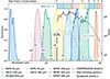 |
Fig. 1. Overview of data used in our analysis. We include transmission curves (left vertical, bottom horizontal axes) for the eight broadband maps used, from Spitzer, Herschel, and SCUBA-2. We overplot the rest-frame wavelengths of selected FIR emission lines, including [CII]-158 μm; these lines are redshifted into the broadband maps. The top horizontal axis labels translate the observer wavelengths into the rest-frame redshift z of a [CII]-158 μm emitter. We trace the z distribution of the COSMOS2020 photometric catalog (in bins of Δz = 0.05), with number counts on the right vertical axis; number counts for the selection of star-forming or quiescent emitters are also shown. Redshifted C+ emission will appear in the SPIRE maps for specific z ranges. Finally, at the top, we demarcate the z-binning used for stacking with LinSimStack; bins at z ∼ 0.65, 1.3, 2.1, and 2.6 were chosen to overlap with the SPIRE bands. |
3. Methods
3.1. Stacking in the confusion limit with LinSimStack
Far-IR or submillimeter observations from single-dish telescopes, such as the maps discussed in Section 2, are restricted in angular resolution, resulting in the so-called “confusion limit”. Simultaneous stacking has been shown to overcome the clustering bias inherent in stacking on maps dominated by confusion noise (Viero et al. 2013, 2022), unlike conventional postage-stamp stacking (mean or median) that is prone to wavelength-dependent biases.
We modeled a broadband map mλ (in Jy/beam, indexed by the mean band wavelength λ) as a linear combination of several sub-maps or layers, each layer Az, m being a convolution of the instrument beam with a hits-map of a portion or bin of the galaxy catalog. The binning was user-defined and based on properties that determine emission in that band, such that stacking with these homogeneous sources gives a meaningful result. The coefficients  , thus regressed, give the average flux density of emitters in that bin or layer:
 (1)
(1)
 (2)
(2)
where W is the weight matrix, given by the inverse per-pixel variance in the broadband maps, and ϵ is the corresponding Gaussian noise vector. The linearity of the regressed parameters  can be exploited to write down a closed form for the least-squares minimization problem.
For our application, we developed LinSimStack6 as a fork of the previously introduced Python-based SIMSTACK3 (Viero et al. 2022). Our version addresses inefficiencies in the SIMSTACK3 codebase, notably exploiting this linearity by analytically marginalizing over the coefficients, instead of using a Levenberg-Marquardt non-linear solver, resulting in order-of-magnitude gains in speed with LinSimStack7. This also enables us to analytically estimate the statistical covariance (see Section 3.2).
We also implemented the following additions, some of which have been utilized in previous work. We included an additive flat foreground layer in Eq. (1) to mitigate biases from mean subtraction of the maps or galactic foreground contamination. We additionally followed Duivenvoorden et al. (2020) to model the leakage of flux from masked areas due to large beams; we added another layer that is the beam convolved with the masked pixels of the galaxy catalog. All redshift and stellar mass bins were simultaneously stacked to reduce any bias due to interlopers (Sun et al. 2018). Finally, linear least-squares fitting was performed twice, with bright outlier pixels removed in the second iteration to reduce positive bias from close interlopers or bad pixels.
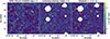 |
Fig. 2. Zoom-in on the stacking outputs for the Herschel/SPIRE 250 μm COSMOS map, illustrating our forward modeling LinSimStack methodology. Left to right: 2D vectors for the data d, model m, and the residuals r = d − m. The model m is a linear combination of all beam-convolved hit-maps constructed using the COSMOS2020 photometric catalog. We also plot sources from the Herschel/SPIRE Point Source Catalog (HSPSC) with estimated fluxes in the HSPSC above 30 mJy, which correlate with the residual flux in the 2D vector r (see Section 3.4, Appendix A, the corresponding figures, and the discussion for further details on model incompleteness). |
We binned our galaxy catalog based on three observables, which are expected to result in similar spectral energy distributions (SEDs) in the thermal IR (Schreiber et al. 2018). We divided the sample into star-forming and quiescent emitters using the rest-frame two-color NUV − r versus R − J criterion, formulated in Ilbert et al. (2013), Arnouts et al. (2013) and used by Weaver et al. (2022), Viero et al. (2022). We binned by redshift z = 0.01 − 6, both because the SED is redshifted and galaxy rest-frame emission changes with cosmic evolution; relevant bin edges in z were selected to match the full width at half maximum (FWHM) of the Herschel/SPIRE transmission (see top of Fig. 1). Finally, we binned the catalog by the (logarithm of) stellar mass log(M/M⊙), as it is a good tracer of IR properties (Viero et al. 2013, 2022). Although Viero et al. (2022) only works with log(M/M⊙) = 9.5 − 12, we binned across a larger range, 8.5 − 13, as we aim for the catalog to describe as much FIR emission as possible with COSMOS20208. Our bin definitions and the corresponding number counts per bin are detailed in Tables D.1 and D.2 for the star-forming and quiescent samples, respectively. We empirically find that increasing the total number of sources by including higher redshifts or lower stellar masses does not improve completeness metrics (fraction of the CIB resolved; Section 3.4)
3.2. Unbiased error estimation
We estimated errors in the average emission flux,  , measured by LinSimStack using the following four independent methods, and conservatively combined them to obtain a final variance in
  .
.
3.2.1. Linear formulation:
For the linear least-squares problem, the statistical covariance has the analytical form  . This provides a robust lower bound for the complete error in
  , as it reflects the random error limit resulting from the covariance of the map pixels, but does not include any information about systematics.
3.2.2. Pixel bootstrapping:
Similarly to Duivenvoorden et al. (2020), we randomly selected 80% of the unmasked pixels and performed the least-squares stacking algorithm ten times to randomly resample the pixels in each map, corresponding to different instrumental noise realizations.
3.2.3. Catalog bootstrapping:
We followed (Viero et al. 2022) and ran ten iterations with 80%:20% split bootstrapping on the catalog, doubling the number of bins while still fitting all emitters available to prevent negatively biasing the fluxes. Galaxy bootstrapping also captures the noise-realization variation encoded by pixel bootstrapping; the variance in  when randomly sampling over galaxies is expected to be higher than when pixel sampling.
3.2.4. Jack-knifing:
Similarly to Duivenvoorden et al. (2020), for a given map, we reran our stacking algorithm four times, with each quartile of the map masked for one run. This encapsulates sample, or cosmic, variance at the scale of the field (≲2 sq. deg.).
Figure 3 shows the fractional error estimates in the mean stacked fluxes using these four individual methods. The uncertainty in  is one of two direct contributors to the constraining power on [CII] emission, the other being the uncertainty in the SED fit (see Sections 3.3 and 3.5). Empirically, the overall uncertainty in our line emission measurement is moderately more dependent on the stacking flux uncertainty than the SED fit uncertainty. We conservatively selected the quadrature sum of the jackknifing error (which encodes cosmic variance on the field scale) and the maximum of the other three error estimates, to obtain
  for subsequent analyses.
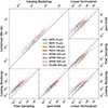 |
Fig. 3. Errors in stacked mean intensities estimated via four methods (see Section 3.2). Fractional errors in the stacked fluxes, obtained as outputs of the LinSimStack are color-coded by band. The statistical lower bound is given by the closed-form error formulation, obtained by writing the stacking problem as a linear regression. Bootstrapping the catalog or the pixels captures the additional systematic errors, as it samples different realizations of pixel noise and emitter variance; empirically, the bootstrapping over the catalog (lower left subplot) typically yields the more conservative error estimates. Jack-knifing (JK) provides an estimate of the cosmic variance (CV) at the scale of the map. We conservatively add in, in quadrature, the JK estimate with the maximum of the other three estimates. This effectively lower-bounds our bootstrapping error estimate by the analytical linear formulation limit. Past analyses (Viero et al. 2022, 2013) have only used catalog bootstrapping as the error estimation method. The main subplot above (top-left) compares our final error estimates with those from catalog bootstrapping alone. Our estimates are more conservative by definition and additionally include a measure of CV. |
3.3. Fitting SED continuum models
We obtained stacked flux densities,  , from Section 3.1 and a diagonal covariance matrix from Section 3.2. The values of
  trace the SED of emitters in each grouped sub-catalog, which is a superposition of several black bodies. This is well modeled (Viero et al. 2013, 2022; Pullen et al. 2018) by a modified black-body function,
 (3)
(3)
where Bν is the nominal Planck function, T is the average dust temperature in the bin, ν0 is the transition between the mid-IR Wien and the Rayleigh-Jeans side. The exponent of the Wien side is given by α, while β is the emissivity index. A single parameter, A, determines the overall amplitude of Sν, with the two functional pieces and their first derivatives required to be equal at ν0 (which removes one degree of freedom and sets ν0). The parameters of the SED model, Θ = (A, α, β, T), were fit to the measured stacked fluxes using the Python MCMC (Markov chain Monte Carlo) package, emcee (Foreman-Mackey et al. 2013), which samples the parameter space to compute the posterior for Θ. We followed Viero et al. (2022) for additional details while computing our Bayesian solution: (a) we used their prescription for initial placement of walkers; (b) flux measurements consistent with zero were treated as upper limits, with their likelihood contribution considered via a survival function (Sawicki 2012); (c) we inflated errors in the stacked MIPS 24 μm measurements, to account for polycyclic aromatic hydrocarbon (PAH) emission in massive galaxies (log M/M⊙ ≥ 10) by factors of 2, 4, and 2.4 for the 0.5 < z < 1.5, 1.5 < z < 2, and 2 < z < 2.5 bins, respectively9. This is identical to Viero et al. (2022).10.
We adopted wide uniform priors for all parameter: log(A)∈𝒰(−10, 0), α ∈ 𝒰(1, 3), β ∈ 𝒰(1, 3), and T ∈ 𝒰(5, 40). These priors are wide and encapsulate prior measurements for the physically meaningful α, β, and T (Casey 2012; Abergel et al. 2014). For stability of the MCMC chains, we defined the overall normalization parameter, A, as the logarithm of the median of the modeled SED values at each of the eight central wavelengths.
3.4. Aggregate IR background as a measure of completeness correction
Within selected frequency bandwidths, we used LinSimStack to measure the integrated average emission from galaxies within a redshift range z and stellar mass m:  . The portion of the CIB resolved by stacking with our catalog can be written as a sum over the bins,
 (4)
(4)
Here, Nz, m is the number of emitters in a given bin. Naively, this can be set to the galaxy counts in COSMOS2020 input to LinSimStack, but this would be a significant underestimate due to incompleteness of the galaxy catalog. Instead, we used completeness-corrected measurements of the stellar mass function (SMF)  , which encode the number density of emitters as a function of stellar mass content, at a given redshift:
 (5)
(5)
 (6)
(6)
 (7)
(7)
 (8)
(8)
Here, the terms, respectively, encode the expected number density of emitters in a given bin, the effective cosmological volume as an integral over the differential comoving volume, and the LinSimStack estimate for mean emission for this kind or bin of emitters. Weaver et al. (2023) measures the SMF for star-forming and quiescent galaxies up to z ≲ 7.5 using COSMOS2020, constraining the parameters of a double and single Schechter function, respectively. We adopted values for the maximum likelihood solution from Tables C.2 and C.3 of Weaver et al. (2023) to compute the expected number of emitters in each bin.
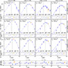 |
Fig. 4. Stacked intensity estimates obtained from LinSimStack for individual COSMOS2020 bins, fit with a modified black-body emission continuum SED model. The top panels of each sub-figure show the stacked mean intensities (blue crosses) and corresponding 1σ envelope of the emcee fits (blue) for a subset of the catalog bins; the bottom panels show the signal-to-noise of the fit residuals. The vertical dashed line represents the wavelength cut, λcut, between the two piecewise components of the SED continuum model in Eq. (3) (i.e., the frequency ν0). For a specific z interval, [CII]-158 μm emission is redshifted into a SPIRE band and manifests as excess residual emission over the continuum; these are marked in orange. The SPIRE 500 μm map contains redshifted [CII]-158 μm from the highest two z bins. Different rows and columns correspond to different stellar mass log(M/M⊙) and redshift z cuts; all bins shown here are from the star-forming selection. The labels indicate the number count within a bin in the catalog and as predicted by the stellar mass function (SMF) from Weaver et al. (2023). We conservatively inflate the variance on the [CII]-158 μm residual emission by the reduced chi-squared, χr2, statistic of each SED fit. The bottom row shows residuals obtained by adding over all bins at the same redshift interval, with potential [CII]-158 μm emission again marked in orange. For brevity, we only show stacking within the three highest stellar mass bins (for each redshift bin with potential [CII]-158 μm emission); these are the predominant contributors to the CIB and [CII]-158 μm emission. (See Appendix B for stacking results in all bins.) The bottom row shows the residuals obtained by adding all stellar mass and star-forming plus quiescent bins at a redshift. |
We report the predicted number counts from the SMF integration in brackets in Tables D.1 and D.2 and select the higher of the two values (from our catalog and the SMF prediction) to prevent underestimation bias at higher redshifts. For the three Herschel/SPIRE maps, in which we report [CII] emission, we resolve approximately 87%, 76%, and 73% of the CIB, compared to Fixsen et al. (1998)’s COBE/FIRAS measurements in the 250 μm, 350 μm, and 500 μm bandpasses11. We scaled the [CII] limits we report (obtained using Eq. (10); see Section 3.5) by an inverse of this completeness fraction, assuming that a similar fraction of the missing cosmic background is [CII] emission12. Potential causes for this incompleteness are discussed further in Appendix A, where we note that LinSimStack fails to resolve some of the brighter sources in the SPIRE maps, which correlate with sources present in the Herschel SPIRE Point Source Catalog (HSPSC). Together, the HSPSC sources in COSMOS account for 10 − 16% of the FIRAS CIB monopole spectrum.
3.5. Aggregate [CII] emission in Herschel/SPIRE maps
We fitted the parameters Θ of a modified black-body SED model, Sz, m(λ; Θ), which provides an estimate of the continuum emission in a given wavelength bin, λ. Redshifted [CII]-158 μm in a SPIRE map appears as residual emission over the fitted continuum
![Mathematical equation: $$ \begin{aligned} S^{\mathrm{[CII]}}_{z, m}(\lambda ) = \bar{S}_{z, m}(\lambda ) - {S}_{z, m}(\lambda ; \Theta ) , \end{aligned} $$](/articles/aa/full_html/2026/01/aa56503-25/aa56503-25-eq22.gif) (9)
(9)
where λ and z are related through the rest-frame emission frequency of [CII]-158 μm, λmap = (1 + z)158 μm. The SPIRE maps thus contain [CII] emission from z ∼ 0.5 − 3, which spans the theorized peak of star formation history.
The total intensity history of line emission is expressed in the same form as Eqs. (7) and (8), with normalization over the COSMOS field (1.6deg2) area necessary to obtain the units of Jy/str:
![Mathematical equation: $$ \begin{aligned} I^{\mathrm{[CII]}}_\nu (z_{\rm [CII]}) = \sum _{z = z_{\rm [CII]}, m} N_{z, m}^\mathrm{SMF-pred} \times S^{\mathrm{[CII]}}_{z, m}(\lambda ). \end{aligned} $$](/articles/aa/full_html/2026/01/aa56503-25/aa56503-25-eq23.gif) (10)
(10)
As noted in Section 3.4, these values are scaled by the completeness fraction, i.e., the fraction of the CIB that our stacking was able to resolve. The uncertainty in the measurement are similar written as
![Mathematical equation: $$ \begin{aligned} \nonumber \sigma \Big (I^{\mathrm{[CII]}}_\nu&(z_{\rm [CII]})\Big ) \\&=\sum _{z = z_{\rm [CII]}, m} N_{z, m}^{\text{ SMF-pred}} \times \sigma \Big (S^{\mathrm{[CII]}}_{z, m}(\lambda )\Big ) \times \sqrt{\chi ^2_{r; z, m}}, \end{aligned} $$](/articles/aa/full_html/2026/01/aa56503-25/aa56503-25-eq24.gif) (11)
(11)
where ![Mathematical equation: $ \sigma(S^{\mathrm{[CII]}}_{z, m}(\lambda)) $](/articles/aa/full_html/2026/01/aa56503-25/aa56503-25-eq25.gif) is the quadrature sum of uncertainties in the two terms of Eq. (9) and χz, m2 is the reduced chi-squared statistic for each SED continuum model (excluding the data point that could contain redshifted [CII] emission). We therefore conservatively scale our [CII] uncertainties by a measure of the goodness of the fit of the model. We note empirically that, for certain galaxy bins, the SED models cannot be well constrained because there are insufficient detections of the mean emissions (i.e., the LinSimStack results are consistent with zero for several broadband maps). For these bins, we did not include a mean emission contribution in (10), but we included an uncertainty contribution in (11) by setting
is the quadrature sum of uncertainties in the two terms of Eq. (9) and χz, m2 is the reduced chi-squared statistic for each SED continuum model (excluding the data point that could contain redshifted [CII] emission). We therefore conservatively scale our [CII] uncertainties by a measure of the goodness of the fit of the model. We note empirically that, for certain galaxy bins, the SED models cannot be well constrained because there are insufficient detections of the mean emissions (i.e., the LinSimStack results are consistent with zero for several broadband maps). For these bins, we did not include a mean emission contribution in (10), but we included an uncertainty contribution in (11) by setting ![Mathematical equation: $ \sigma \Big(S^{\mathrm{[CII]}}_{z, m}(\lambda) \Big) = \sigma\Big(\bar{S}_{z, m}(\lambda)\Big) $](/articles/aa/full_html/2026/01/aa56503-25/aa56503-25-eq26.gif) . These bins contribute ≲0.06% of the FIRAS CIB monopole measurement (i.e., well within our quoted error bars), as they typically contain significantly fewer galaxies.
. These bins contribute ≲0.06% of the FIRAS CIB monopole measurement (i.e., well within our quoted error bars), as they typically contain significantly fewer galaxies.
Constraints on [CII]-158 μm in four tomographic bins.
4. Results and discussion
4.1. [CII]-158 μm constraints
We present our [CII]-158 μm measurements in four tomographic bins in Figure 5 and Table 2. Our constraints are inconsistent with no emission in three of these bins at 1.2 − 1.4σ. We do not obtain a statistically non-zero detection at z ∼ 2.1; our 3σ upper bound is plotted in red in Figure 5. Overall, the quadrature sum of S/N in our four measurements is ∼2.42. These constraints indicate that [CII]-158 μm constitutes no more than 4 − 8% of the CIB (Figure 5 shows the COBE/FIRAS measurement of the monopole CIB spectrum) at the corresponding observed wavelengths (240 − 600 μm).
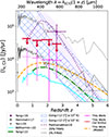 |
Fig. 5. Measurements of [CII]-158 μm at z ∼ 0.3 − 2.9 compared with [CII]-158 μm-LF estimates in the local universe (Hemmati et al. 2017) and z ∼ 5 (Yan et al. 2020). Also shown are theoretical predictions from C+ evolution models, including Gong et al. (2012) (blue hatches), Padmanabhan (2019) (dotted purple: best model, shaded band: uncertainty), Yang et al. (2022) (dash-dotted green), and Béthermin et al. (2022) (cyan line: De Looze et al. 2014 version; cyan dashed: high SFRD version at high z). Our 3σ upper limits disfavor high-temperature collisional excitation frameworks and best-fit empirical models calibrated to the Pullen et al. (2018), Yang et al. (2019)Planck measurement. The 1σ results are more consistent with SFR-scaling models, which calibrate C+ luminosity to the SFR of sources. Additionally, we show the COBE/FIRAS measurement of the monopole spectrum of the CIB as a function of wavelength, matched to the rest-frame redshift of [CII]-158 μm emission. The [CII]-158 μm contribution is likely no more than a few percent of the total CIB, with the intensity history evolving by less than an order of magnitude across cosmic moon. |
We also plot estimates of [CII]-158 μm at z ∼ 0 and z ∼ 6, as well as theoretical predictions from selected C+ models in Figure 5. Yan et al. (2020) combined targeted and serendipitous [CII] detections with IR luminosity functions from the ALPINE survey to estimate the [CII] luminosity function and mean intensity at z ∼ 5. Hemmati et al. (2017) estimated the local [CII] luminosity function by applying scaling relations, derived from the GOALS13 survey of local (ultra) luminous IR galaxies ((U)LIRGs), to a flux-limited sample of IR-selected galaxies from IRAS14, using direct [CII] measurements in place of estimates for the brightest galaxies. We integrated their double-power-law fit to the resulting luminosity function to derive an estimate of the local [CII] luminosity density. We note that neither the z ∼ 0 nor z ∼ 5 measurements are based on a direct measurement of the [CII] luminosity function (LF) and may have significant systematic uncertainties. Nevertheless, we include them as useful indications of the behavior of the mean [CII] intensity outside the redshift interval we measured directly.
To compare our results with theoretical expectations, we replicated predictions for the redshift evolution of [CII]-158 μm from the literature. Yang et al. (2021, 2022) (Y22) calibrate the galaxy ISM line emission luminosity versus halo mass relations to semi-analytical simulations. We reproduce the best model and uncertainties from the Padmanabhan (2019) (Pa19) prescription, which is designed to simultaneously reproduce the Hemmati et al. (2017) and Pullen et al. (2018) measurements. Finally, we included a suite of models from Gong et al. (2012) (G12), which assume that C+ is proportional to the total carbon mass in dark matter halos. The G12 models treat electron kinetic temperature Tke and number density nrme as free parameters and list several models for different pairs; we plotted their range of estimates for their high temperature (log10(Tke/1 K) = 3 − 4, log10(ne/1 cm−3) = 2 − 4) and low temperature (log10(Tke/1 K) = 2, log10(ne/1 cm−3) = 0 − 2) models separately. We also replicated the predicted [CII]-158 μm intensity history from the Simulated Infrared Dusty Extragalactic Sky (SIDES) model (Béthermin et al. 2022) (B22), specifically showing the De Looze et al. (2014) (D14) version with the “high SFRD” variant (shown dashed) at high redshifts.
Finally, we implemented our own SFR-tracing model using the SIMIM modeling framework15. We briefly describe the methodology and refer to Keating et al. (2020), Keenan et al. (2022, 2020), Keenan et al. (in prep.) for additional details. Starting from the magneto-dynamic simulation suite IllustriusTNG, specifically TNG100-1, (Naiman et al. 2018; Springel et al. 2018; Pillepich et al. 2018; Nelson et al. 2018; Marinacci et al. 2018), for each volume at a given redshift, we prescribed a subgrid line emission model, from empirical calibration of subhalo mass to SFR (Behroozi et al. 2013) and constraints on the scaling between [CII] luminosity and SFR (De Looze et al. 2014). Finally, we applied a constant amplitude scaling to best fit the constraints from Hemmati et al. (2017), Yan et al. (2020), and this analysis.
The empirical B22 SIDES-based model constructed above and the Y22 semi-analytical models imply a close connection between [CII] and star formation, and we designate them broadly as “SF-tracing.” Conversely, the G12 model requires no connection between [CII] and SFR, while the Pa19 model relies on a more-than-linear redshift evolution of [CII]-SFR correlation to reproduce the Pullen et al. (2018) data point. Our 3σ limits are inconsistent with the best-fit Pa19 model and with all high-temperature versions of the G12 prescription at all z. We excluded the low-temperature G12 models at 3σ in our lowest redshift bin, z ∼ 0.65, with some models falling within our 1σ bar at higher redshifts. Lower-intensity versions within the uncertainty range of the Pa19 model space are also within the 3σ limits. The predictions of the SF-tracing models lie well within the upper limits and are consistent within the 1σ uncertainty bars. Our measurements therefore disfavor scenarios in which the ratio between [CII] luminosity and SFR evolves dramatically across cosmic noon. Our results from this untargeted survey are consistent with targeted studies that have found near-linear scaling between [CII] luminosity and SFR with little to no redshift evolution (De Looze et al. 2014; Schaerer et al. 2020; Romano et al. 2022), although higher sensitivities would be required for a robust confirmation.
Estimated bias from contaminating spectral lines within the Herschel/SPIRE broad bandpass for each [CII]-158 μm redshift bin.
In the nearby Universe, (U)LIRGS exhibit low L[CII]/LIR ratios (L[CII] and LIR being the [CII]-158 μm line luminosity and the IR luminosity, respectively), relative to non-IR-selected samples (Díaz-Santos et al. 2017). At cosmic noon, around half of star formation occurs in (U)LIRGS (Casey et al. 2014), implying that a significant fraction of the mean [CII]-158 μm intensity must also originate in such systems. To check for evidence that galaxies contributing significantly to Iν[CII] at 0.33 < z < 2.9 are [CII] deficient, we computed the ratio of the integrated [CII] and total IR (TIR) luminosities in each redshift bin. To achieve this, we calculated the luminosity-weighted integral of the IR luminosity functions of Gruppioni et al. (2013)16 at the central redshift of each bin and computed the ratio with Iν[CII](z) (converted into units of L⊙ Mpc−3). Figure 6 compares our constraints on L[CII]/LIR with the ratios for local SFGs and (U)LIRGS observed by Herschel, derived from Accurso et al. (2017) and Díaz-Santos et al. (2017), respectively. Taking the variance-weighted average of all redshift bins yields L[CII]/LIR = 0.0053 ± 0.0023, which is very similar to the value observed in SFGs in the nearby Universe. Our constraint lies 2σ above the median ratio seen in (U)LIRGs. This suggests that the galaxies that make up the bulk of the [CII] emission at cosmic noon do not exhibit large [CII] deficits; however, confirmation with more sensitive data is required. While our data only constrain the L[CII]/LIR ratios for galaxies responsible for the bulk of FIR emission at these redshifts, our findings are consistent with Zanella et al. (2018), who show that z ∼ 2 SFGs do not exhibit deficient L[CII]/LIR ratios, despite their (U)LIRG-like total IR luminosities.
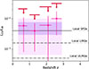 |
Fig. 6. Population-average [CII]-to-IR luminosity ratios, derived comparing our [CII] constraints with integrated IR luminosity function of Gruppioni et al. (2013). Red limits and pink crosses indicate 3σ upper bounds and 1σ intervals in each redshift bin. Purple bars show the variance-weighted average over all bins (z ∼ 0.33 − 2.9), with dark purple and light purple indicating 1σ and 2σ intervals. We also show the average ratios for local SFGs from [CII] observations from Accurso et al. (2017), and for LIRGs and ULIRGs from Díaz-Santos et al. (2017). |
4.2. Contaminating spectral lines
[CII]-158 μm is not the only narrow non-continuum spectral feature in these bands, and other emission lines can originate from (and hence correlate with) galaxies within our specified z bins. Thus, some of the excess emission we measure over the continuum could originate from lines other than [CII]-158 μm.
To estimate this positive bias on our [CII]-158 μm measurement, we considered all emission lines listed in Table 1 of Visbal et al. (2011). The table lists the rest-frame wavelengths of each line, along with a calibration ratio between line luminosity and SFR  . We assume that the ratio of the luminosities of the [CII]-158 μm and the interloper line (denoted by “inter”) is given by the ratio of their luminosity–SFR calibration factors,
![Mathematical equation: $$ \begin{aligned} L_{\rm inter} \Big / L_{\rm [CII]} = R_{\rm inter} \Big / R_{\rm [CII]}. \end{aligned} $$](/articles/aa/full_html/2026/01/aa56503-25/aa56503-25-eq29.gif) (12)
(12)
Pullen et al. (2018) also estimate interloper bias on their measurements using the same table under a similar assumption for line luminosity scaling.
Next, given the transmission T(λ) of each SPIRE map’s broadband filter (see Fig. 1), we computed the effective transmission coefficient for each contaminant line within each redshift bin in Table 2. Contaminant emission from interloper lines in our measurement is thus17
 (13)
(13)
where the two terms respectively encapsulate the proportional brightness of the line being constrained ([CII]-158 μm) and the relative overlap of interloper line emission at the correct redshifts and wavelengths, which we optimized for in our binning (as discussed in Section 3.1 and Fig. 1).
Table 3 lists each of the bins in which we report a [CII] constraint, the redshift ranges, lines from the collection in Visbal et al. (2011) that are redshifted into the FWHM of the corresponding SPIRE map, and finally, an estimate of the fraction of the excess emission we measure that could be attributed to emission from non-[CII]-158 μm lines. The main contaminants are [OI]-145 μm, as it is very close to the rest-frame wavelength of the [CII] line, and [NII]-122 μm, whose overall line luminosity is expected to be within an order of magnitude of [CII]-158 μm (Visbal et al. 2011). Overall, we expect contamination from interlopers to be within 6.5 − 11% of the measured total excess emission; we consider the effects on our reported (∼1 − 1.4σ significance) results subdominant.
Mapping FIR fields at higher spectral resolution would be the obvious way forward to address contaminants, lowering the effective transmission,  , for interlopers in Eq. (13). It is noteworthy for the discussion in Section 4.4 that correcting for the effect of contaminants would lower our result, increasing the tension with the Planck×BOSS results.
4.3. Other systematics
We briefly discuss other potential systematics in our best estimates and in the 3σ upper limits.
4.3.1. Photometric redshift uncertainty:
The COSMOS2020 photometric galaxy catalog claims sub-percent accuracy for bright objects in the i-band (i < 21) and < 5% precision for the faintest (25 < i < 27) sources (Weaver et al. 2022). As our broadband filters and corresponding z-bins are wide, we do not expect photo-z errors to significantly and systematically move galaxies with [CII]-158 μm emission into neighboring bins. To quantify the effects of z errors, we generated the same catalog used in the analysis above, except sampling the estimated photometric z from a skewed Gaussian distribution that replicates the median, lower 68%, and upper 68% of the probability distribution functions (z-PDFs) in the COSMOS2020 catalog. We reran our stacking and SED fitting analysis on this catalog with the modified sampled redshifts. We find that our [CII]-158 μm constraints deviate by no more than 0.09σ in any of the four z bins, which we consider sub-dominant to our measurements.
4.3.2. Diffuse emission from intergalactic medium and unmodeled extragalactic background light:
Our stacking methodology measures [CII]-158 μm emission from physical scales within the Herschel beam of the sources in the COSMOS2020 catalog, which is ∼0.2 − 1 cMpc at z ∼ 0.3 − 2.9. We expect this to account for the circumgalactic medium and the diffuse [CII] halo around sources, which are typically within ≲100 kpc. (Tumlinson et al. 2017; Fujimoto et al. 2019, 2020; Lambert et al. 2023; Ikeda et al. 2025; Herrera-Camus et al. 2015) Our results could be negatively biased due to underestimating emission from the large-scale diffuse intergalactic medium (IGM). However, this effect is subdominant, as the mean [CII]-158 μm emission from the IGM is expected to be orders of magnitude lower than galaxies (Gong et al. 2012).
The emission in the Herschel/SPIRE bands can be resolved entirely (within error bars) via source stacking in the COSMOS field (Duivenvoorden et al. 2020). However, notably, their catalog is non-tomographic, and we can only stack the subset with photo-z estimates in this analysis. Section 3.4 describes the corrections we applied to account for the unmodeled background in the FIR, which included modifications based on stellar mass function (SMF) measurements, as well as a constant scaling to match the COBE/FIRAS monopole spectrum. Invalidity of the assumptions underlying these two extrapolations would bias our measurement. Potentially more complete photo-z catalogs exist, such as COSMOS2025 (Shuntov et al. 2025), but they cover smaller portions of the sky, resulting in reduced sensitivity when stacking.
4.4. Tension with past constraints at z ∼ 2.6
In Figure 7, we directly compare our measurements with the Pullen et al. (2018), Yang et al. (2019) constraint at z ∼ 2.6. In their analyses, Y19+P18 cross-correlate quasars and CMASS galaxies from SDSS BOSS with three high-frequency IR all-sky maps from the Planck mission. This enables a search for excess emission in the middle 545 GHz band, with the cross-power spectrum in the 353–857 GHz bands constraining nuisance parameters, including the CIB and the thermal Sunyaev-Zeldovich contribution. This excess emission is theorized to be [CII]-158 μm, expected to be the brightest line feature in the band. Previous measurements by Y19+P18 indicate ![Mathematical equation: $ I^{\mathrm{[CII]}}_\nu \sim 69^{+42}_{-38} $](/articles/aa/full_html/2026/01/aa56503-25/aa56503-25-eq32.gif) kJy/sr at 95% C.L., amounting to ∼10 − 30% of the CIB at 545 GHz. Our measurement in the z ∼ 2.6 tomographic bin is ∼7.5× smaller and inconsistent at about 2.9σ. Notably, our 3σ upper bound at 29 kJy/sr is still below the 95% confidence lower limit reported by Y19+P18.
kJy/sr at 95% C.L., amounting to ∼10 − 30% of the CIB at 545 GHz. Our measurement in the z ∼ 2.6 tomographic bin is ∼7.5× smaller and inconsistent at about 2.9σ. Notably, our 3σ upper bound at 29 kJy/sr is still below the 95% confidence lower limit reported by Y19+P18.
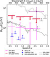 |
Fig. 7. Constraints with 3σ upper bounds vs. 95% C.L. bounds from Yang et al. (2019) (a followup of Pullen et al. (2018)) measurement at z ∼ 2.6. No [CII]-158 μm is detected at the previously tentatively reported levels; our best estimates are ∼7.5× lower, with the other 3σ upper bound at z ∼ 2.6 lower than the 95% C.L. interval. Expected 3σ sensitivity limits of two in-development surveys (Pullen et al. 2023; Bracks et al., in prep.) which will measure C+ at high R, are also shown. This tension is discussed further in the text (Section 4). |
Assuming the validity of either analysis, we discuss the physics or systematics that could explain this 2.9σ tension and inconsistency of nearly an order of magnitude in the [CII]-158 μm intensity history just prior to the peak of cosmic star formation. The Y19+P18 studies cross-correlate all-sky fields, utilizing scales as large as multipole moment l ∼ 100 (or angular scales of ∼1deg). Therefore, they explore cross-correlation at larger scales than the Herschel/SPIRE beam at ∼500 μm, which corresponds to ∼1 cMpc at z ∼ 2.6. As discussed in Section 4.3, if C+ predominantly exists outside of ∼1 cMpc of sources, our analysis would underestimate [CII]-158 μm, but line emission would still correlate at large scales in Planck maps and Y19+P18 would detect it. However, Gong et al. (2012) models the IGM [CII]-158 μm contribution to be orders of magnitude lower than that of galaxies.
Our analysis uses a photometric catalog that is incomplete; as discussed in Section 3.4, we measured and attempted to correct for this incompleteness. We scaled our [CII]-158 μm measurements by the inverse of the fraction of the COBE/FIRAS CIB monopole spectrum that we resolve; this assumes an underlying extrapolation that the same fraction of the emission from sources not in our photometric catalog is [CII]. Our measurements would therefore be an underestimation if sources missing from the COSMOS2020 photometric redshift catalog were anomalously bright emitters of [CII]-158 μm. However, it is worth pointing out that we only miss ∼15 − 25% of the CIB in the SPIRE bands; thus, a significant portion of the IR emission from the missing sources would have to be [CII] to account for the tension with Y19+P18, which posits ∼20% of the CIB to be [CII]-158 μm.
Examining the final column of Figure 4 (or Figure 7 from Pullen et al. (2018)), we note that Y19+P18 uses three points, all > 350 μm, to constrain a similar continuum SED model as our analysis; empirically, using a low number of samples only on the Rayleigh-Jean side of the modified black-body model could be prone to fitting and numerical systematics. More data points at wavelengths away from the bands in which [CII] emission would enable an analysis like ours to robustly constrain the nuisance SED parameters.
4.5. Future outlook
Figure 7 also presents sensitivity forecasts for two in-development instruments. We include the 3σ noise limits expected from cross-correlating datasets from two C+ spectrometers with a respective ancillary galaxy catalog. The Terahertz Intensity Mapper (TIM; Vieira et al. (2020)) is a balloon-borne FIR spectrometer, with spectral resolution R ∼ 250, mapping a deep field at GOODS-South for O(100) hours. The field observed by TIM overlaps with the Euclid Deep Field Fornax (EDFF); TIM plans to cross-correlate their [CII]-158 μm maps at z ∼ 0.5 − 1.5 with the deep high number-count Euclid spectroscopic galaxy catalog (Bracks et al., in prep.). The EXperiment for Cryogenic Large-Aperture Intensity Mapping (EXCLAIM) (Pullen et al. 2023) will map [CII]-158 μm at z ∼ 2.5 − 3.5 over an equatorial field for ∼10 hours. The experiment plans to cross-correlate with the SDSS BOSS spectroscopic redshift catalog. Figure 7 shows that if either experiment is able to reach its predicted sensitivity, it will be a step towards resolving this perceived tension by detecting [CII] at several σ.
Constraints from our methodology can be improved by increasing either the depth of the FIR broadband maps, the number counts in the galaxy catalog, or by addressing systematics with smaller photo-z uncertainty or narrower bandpass measurements. We are currently limited to broadband mapping instruments of the past, such as Herschel and Spitzer, but wider and/or more complete galaxy catalogs are imminent. Deeper UV-O-IR measurements of COSMOS, such as with JWST/NIRCam or JWST/MIRI (Casey et al. 2023; Shuntov et al. 2025), could improve the FIR completeness of our forward model. More promisingly, galaxy catalogs with the same depth but more overlap with the Herschel deep fields, e.g., Euclid photometry and spectra (Mellier et al. 2025; Jahnke et al. 2025), would decrease our constraint variance as roughly inversely proportional to the total number counts of emitters with photo-z in the coinciding regions.
5. Conclusions
We place the first constraints on [CII]-158 μm emission during and immediately after the peak of star formation history, at z ∼ 0.6 − 2. These results imply that [CII]-158 μm emission increased by roughly an order of magnitude from z ∼ 5 and then fell by a similar amount to the present day, accounting for no more than a few percent of the cosmic IR background at its peak. Our measurements, with a total S/N of 2.42, imply Iν[CII] of ∼10 kJy/sr across z ∼ 0.6 − 2.6.
We are unable to replicate measurements at z ∼ 2.6 obtained from cross-correlating Planck IR maps with quasars from the wide spectroscopic survey BOSS. Experiments currently in development, TIM and EXCLAIM, are forecasted to be sensitive enough to address this tension and measure [CII] at several σs. Additionally, imminent data releases of the deep-field galaxy catalogs from the recently launched Euclid mission, as well as the COSMOS-Web survey, are expected to yield higher-completeness coverage over larger fields overlapping with Herschel deep maps. A future extension of our analysis with Euclid redshifts could leverage such higher effective number counts to decrease uncertainties on stacked fluxes, and thus Iν[CII].
We have demonstrated a search for FIR line emission in deep field multi-wavelength surveys, using LinSimStack, a faster linearized version of previously introduced stacking utilities. It is straightforward to extend our analysis to obtain complementary constraints from different datasets, such as Euclid, and from different fields, such as GOODS. Our methodology can also be used to constrain the redshift evolution of molecular lines from CO, [OI], [OIII], and N+, provided that these narrow spectral features are expected to be significantly brighter than contaminating interlopers, or that maps at higher spectral resolution are available.
Acknowledgments
We thank Garrett Keating, Adam Lidz, Ian Smail, Joaquin Vieira, and Jessica Zebrowski for insightful discussion. We thank the anonymous reviewer for their comments. The S2CLS JCMT data used in this paper were taken as part of Program ID MJLSC02. This publication was made possible through the support of Grant 63040 from the John Templeton Foundation. The opinions expressed in this publication are those of the authors and do not necessarily reflect the views of the John Templeton Foundation. Shubh Agrawal’s work was also supported by the Quad Fellowship. Facilities: COSMOS2020 (Weaver et al. 2022): GALEX, MegaCam/CFHT, ACS/HST, HSC/Subaru, Suprime-Cam/Subaru, VIRCAM/VISTA, IRAC/Spitzer; Maps: MIPS/Spitzer, SPIRE/Herschel, PACS/Herschel, SCUBA2/JCMT. Software: astropy (Astropy Collaboration 2013, 2018); emcee (Foreman-Mackey et al. 2013), LinSimStack, an fork of SIMSTACK3 (Viero et al. 2022, 2013)
References
- Abergel, A., Ade, P. A. R., Aghanim, N., et al. 2014, A&A, 571, A11 [NASA ADS] [CrossRef] [EDP Sciences] [Google Scholar]
- Accurso, G., Saintonge, A., Catinella, B., et al. 2017, MNRAS, 470, 4750 [NASA ADS] [Google Scholar]
- Arnouts, S., Le Floc’h, E., Chevallard, J., et al. 2013, A&A, 558, A67 [NASA ADS] [CrossRef] [EDP Sciences] [Google Scholar]
- Astropy Collaboration (Robitaille, T. P., et al.) 2013, A&A, 558, A33 [NASA ADS] [CrossRef] [EDP Sciences] [Google Scholar]
- Astropy Collaboration (Price-Whelan, A. M., et al.) 2018, AJ, 156, 123 [Google Scholar]
- Behroozi, P. S., Wechsler, R. H., & Conroy, C. 2013, ApJ, 770, 57 [NASA ADS] [CrossRef] [Google Scholar]
- Béthermin, M., Dole, H., Beelen, A., & Aussel, H. 2010, A&A, 512, A78 [NASA ADS] [CrossRef] [EDP Sciences] [Google Scholar]
- Béthermin, M., Le Floc’h, E., Ilbert, O., et al. 2012, A&A, 542, A58 [NASA ADS] [CrossRef] [EDP Sciences] [Google Scholar]
- Béthermin, M., Gkogkou, A., Van Cuyck, M., et al. 2022, A&A, 667, A156 [NASA ADS] [CrossRef] [EDP Sciences] [Google Scholar]
- Casey, C. M. 2012, MNRAS, 425, 3094 [Google Scholar]
- Casey, C. M., Narayanan, D., & Cooray, A. 2014, Phys. Rep., 541, 45 [Google Scholar]
- Casey, C. M., Kartaltepe, J. S., Drakos, N. E., et al. 2023, ApJ, 954, 31 [NASA ADS] [CrossRef] [Google Scholar]
- CCAT-Prime Collaboration (Aravena, M., et al.) 2022, ApJS, 264, 7 [NASA ADS] [Google Scholar]
- Crawford, M. K., Genzel, R., Townes, C. H., & Watson, D. M. 1985, ApJ, 291, 755 [Google Scholar]
- De Looze, I., Cormier, D., Lebouteiller, V., et al. 2014, A&A, 568, A62 [NASA ADS] [CrossRef] [EDP Sciences] [Google Scholar]
- Devlin, M. J., Ade, P. A. R., Aretxaga, I., et al. 2009, Nature, 458, 737 [NASA ADS] [CrossRef] [Google Scholar]
- Díaz-Santos, T., Armus, L., Charmandaris, V., et al. 2017, ApJ, 846, 32 [Google Scholar]
- Dole, H., Lagache, G., Puget, J.-L., et al. 2006, A&A, 451, 417 [NASA ADS] [CrossRef] [EDP Sciences] [Google Scholar]
- Duivenvoorden, S., Oliver, S., Béthermin, M., et al. 2020, MNRAS, 491, 1355 [Google Scholar]
- Dunne, D. A., Cleary, K. A., Breysse, P. C., et al. 2024, ApJ, 965, 7 [NASA ADS] [CrossRef] [Google Scholar]
- Fixsen, D., Dwek, E., Mather, J., Bennett, C., & Shafer, R. 1998, ApJ, 508, 123 [NASA ADS] [CrossRef] [Google Scholar]
- Fonseca, J., Silva, M. B., Santos, M. G., & Cooray, A. 2017, MNRAS, 464, 1948 [NASA ADS] [CrossRef] [Google Scholar]
- Foreman-Mackey, D., Hogg, D. W., Lang, D., & Goodman, J. 2013, PASP, 125, 306 [Google Scholar]
- Fujimoto, S., Ouchi, M., Ferrara, A., et al. 2019, ApJ, 887, 107 [Google Scholar]
- Fujimoto, S., Silverman, J. D., Bethermin, M., et al. 2020, ApJ, 900, 1 [Google Scholar]
- Geach, J. E., Dunlop, J. S., Halpern, M., et al. 2017, MNRAS, 465, 1789 [Google Scholar]
- Gong, Y., Cooray, A., Silva, M., et al. 2012, ApJ, 745, 49 [NASA ADS] [CrossRef] [Google Scholar]
- Gruppioni, C., Pozzi, F., Rodighiero, G., et al. 2013, MNRAS, 432, 23 [Google Scholar]
- Hemmati, S., Yan, L., Diaz-Santos, T., et al. 2017, ApJ, 834, 36 [Google Scholar]
- Herrera-Camus, R., Bolatto, A. D., Wolfire, M. G., et al. 2015, ApJ, 800, 1 [Google Scholar]
- Ikeda, R., Tadaki, K.-I., Mitsuhashi, I., et al. 2025, A&A, 693, A237 [NASA ADS] [CrossRef] [EDP Sciences] [Google Scholar]
- Ilbert, O., McCracken, H. J., Le Fèvre, O., et al. 2013, A&A, 556, A55 [NASA ADS] [CrossRef] [EDP Sciences] [Google Scholar]
- Jahnke, K., Gillard, W., Schirmer, M., et al. 2025, A&A, 697, A3 [Google Scholar]
- Karkare, K. S., Moradinezhad Dizgah, A., Keating, G. K., Breysse, P., & Chung, D. T. 2022, ArXiv e-prints [arXiv:2203.07258] [Google Scholar]
- Keating, G. K., Bower, G. C., Marrone, D. P., et al. 2015, ApJ, 814, 140 [NASA ADS] [Google Scholar]
- Keating, G. K., Marrone, D. P., Bower, G. C., & Keenan, R. P. 2020, ApJ, 901, 141 [NASA ADS] [CrossRef] [Google Scholar]
- Keenan, R. P., Marrone, D. P., & Keating, G. K. 2020, ApJ, 904, 127 [NASA ADS] [CrossRef] [Google Scholar]
- Keenan, R. P., Keating, G. K., & Marrone, D. P. 2022, ApJ, 927, 161 [Google Scholar]
- Lambert, T. S., Posses, A., Aravena, M., et al. 2023, MNRAS, 518, 3183 [Google Scholar]
- Liang, L., Feldmann, R., Murray, N., et al. 2024, MNRAS, 528, 499 [NASA ADS] [CrossRef] [Google Scholar]
- Loiacono, F., Decarli, R., Gruppioni, C., et al. 2021, A&A, 646, A76 [EDP Sciences] [Google Scholar]
- Madau, P., & Dickinson, M. 2014, ARA&A, 52, 415 [Google Scholar]
- Magnelli, B., Elbaz, D., Chary, R. R., et al. 2011, A&A, 528, A35 [NASA ADS] [CrossRef] [EDP Sciences] [Google Scholar]
- Marinacci, F., Vogelsberger, M., Pakmor, R., et al. 2018, MNRAS, 480, 5113 [NASA ADS] [Google Scholar]
- Mellier, Y., Abdurro’uf, Acevedo Barroso, J. A., et al. 2025, A&A, 697, A1 [Google Scholar]
- Moradinezhad Dizgah, A., & Keating, G. K. 2019, ApJ, 872, 126 [Google Scholar]
- Naiman, J. P., Pillepich, A., Springel, V., et al. 2018, MNRAS, 477, 1206 [Google Scholar]
- Nelson, D., Pillepich, A., Springel, V., et al. 2018, MNRAS, 475, 624 [Google Scholar]
- Olsen, K., Greve, T. R., Narayanan, D., et al. 2017, ApJ, 846, 105 [Google Scholar]
- Padmanabhan, H. 2019, MNRAS, 488, 3014 [CrossRef] [Google Scholar]
- Patel, H., Clements, D. L., Vaccari, M., et al. 2013, MNRAS, 428, 291 [Google Scholar]
- Pillepich, A., Nelson, D., Hernquist, L., et al. 2018, MNRAS, 475, 648 [Google Scholar]
- Pullen, A. R., Serra, P., Chang, T.-C., Doré, O., & Ho, S. 2018, MNRAS, 478, 1911 [NASA ADS] [CrossRef] [Google Scholar]
- Pullen, A. R., Breysse, P. C., Oxholm, T., et al. 2023, MNRAS, 521, 6124 [NASA ADS] [CrossRef] [Google Scholar]
- Romano, M., Morselli, L., Cassata, P., et al. 2022, A&A, 660, A14 [NASA ADS] [CrossRef] [EDP Sciences] [Google Scholar]
- Sawicki, M. 2012, PASP, 124, 1208 [NASA ADS] [CrossRef] [Google Scholar]
- Schaerer, D., Ginolfi, M., Béthermin, M., et al. 2020, A&A, 643, A3 [NASA ADS] [CrossRef] [EDP Sciences] [Google Scholar]
- Schreiber, C., Elbaz, D., Pannella, M., et al. 2018, A&A, 609, A30 [NASA ADS] [CrossRef] [EDP Sciences] [Google Scholar]
- Scoville, N., Aussel, H., Brusa, M., et al. 2007, ApJS, 172, 1 [Google Scholar]
- Serra, P., Doré, O., & Lagache, G. 2016, ApJ, 833, 153 [NASA ADS] [CrossRef] [Google Scholar]
- Shirley, R., Duncan, K., Campos Varillas, M. C., et al. 2021, MNRAS, 507, 129 [NASA ADS] [CrossRef] [Google Scholar]
- Shuntov, M., Akins, H. B., Paquereau, L., et al. 2025, COSMOS2025: The COSMOS-Web Galaxy Catalog of Photometry, Morphology, Redshifts, and Physical Parameters from JWST, HST, and Ground-based Imaging [Google Scholar]
- Silva, M., Santos, M. G., Cooray, A., & Gong, Y. 2015, ApJ, 806, 209 [NASA ADS] [CrossRef] [Google Scholar]
- Springel, V., Pakmor, R., Pillepich, A., et al. 2018, MNRAS, 475, 676 [Google Scholar]
- SSC and IRSA 2020, Spitzer Enhanced Imaging Products (SEIP) [Google Scholar]
- Stacey, G. J., Geis, N., Genzel, R., et al. 1991, ApJ, 373, 423 [NASA ADS] [CrossRef] [Google Scholar]
- Sun, G., Moncelsi, L., Viero, M. P., et al. 2018, ApJ, 856, 107 [NASA ADS] [CrossRef] [Google Scholar]
- Tumlinson, J., Peeples, M. S., & Werk, J. K. 2017, ARA&A, 55, 389 [Google Scholar]
- Vallini, L., Gallerani, S., Ferrara, A., Pallottini, A., & Yue, B. 2015, ApJ, 813, 36 [NASA ADS] [CrossRef] [Google Scholar]
- Vieira, J., Aguirre, J., Bradford, C. M., et al. 2020, The Terahertz Intensity Mapper (TIM) a Next-Generation Experiment for Galaxy Evolution Studies [Google Scholar]
- Viero, M. P., Moncelsi, L., Quadri, R. F., et al. 2013, ApJ, 779, 32 [NASA ADS] [CrossRef] [Google Scholar]
- Viero, M. P., Moncelsi, L., Quadri, R. F., et al. 2015, ApJ, 809, L22 [NASA ADS] [CrossRef] [Google Scholar]
- Viero, M. P., Sun, G., Chung, D. T., Moncelsi, L., & Condon, S. S. 2022, MNRAS, 516, L30 [NASA ADS] [CrossRef] [Google Scholar]
- Visbal, E., Trac, H., & Loeb, A. 2011, JCAP, 2011, 010 [Google Scholar]
- Weaver, J. R., Kauffmann, O. B., Ilbert, O., et al. 2022, ApJS, 258, 11 [NASA ADS] [CrossRef] [Google Scholar]
- Weaver, J. R., Davidzon, I., Toft, S., et al. 2023, A&A, 677, A184 [NASA ADS] [CrossRef] [EDP Sciences] [Google Scholar]
- Wilson, D., Cooray, A., Nayyeri, H., et al. 2017, ApJ, 848, 30 [NASA ADS] [CrossRef] [Google Scholar]
- Yan, L., Sajina, A., Loiacono, F., et al. 2020, ApJ, 905, 147 [Google Scholar]
- Yang, S., Pullen, A. R., & Switzer, E. R. 2019, MNRAS, 489, L53 [CrossRef] [Google Scholar]
- Yang, S., Somerville, R. S., Pullen, A. R., et al. 2021, ApJ, 911, 132 [NASA ADS] [CrossRef] [Google Scholar]
- Yang, S., Popping, G., Somerville, R. S., et al. 2022, ApJ, 929, 140 [NASA ADS] [CrossRef] [Google Scholar]
- Yue, B., Ferrara, A., Pallottini, A., Gallerani, S., & Vallini, L. 2015, MNRAS, 450, 3829 [NASA ADS] [CrossRef] [Google Scholar]
- Zanella, A., Daddi, E., Magdis, G., et al. 2018, MNRAS, 481, 1976 [Google Scholar]
Cosmic Evolution Survey.
Spitzer Enhanced Imaging Products.
Herschel Extragalactic Legacy Project.
Submillimetre Common-User Bolometer Array 2; https://zenodo.org/records/57792
https://github.com/shubhagrawal30/LinSimStack
Other improvements included code profiling and refactoring to improve time and memory complexity bottlenecks; discussion of these is outside the scope of this work and further implementation details are available on GitHub.
Note that Duivenvoorden et al. (2020) were able to resolve a large fraction of the CIB with sources that are part of the COSMOS2020 catalog; unlike their analysis, we do have to exclude a portion that does not have estimates for photometric redshifts.
We point out that PAH emission, mostly 3 − 20 μm rest wavelengths, is expected to significantly contaminate only the MIPS 24 μm map. Constraining the fitted temperature of the continuum SED was an integral goal of the Viero et al. (2022) analysis, making biases in their lowest wavelength band crucial. However, given that the SPIRE bands lie predominantly on the Rayleigh-Jeans side of the SED, we do not expect uncertainty in the 24 μm stacking measurement to significantly affect our residual measurement.
These completeness fractions are lower than in the Duivenvoorden et al. (2020) analysis of the COSMOS field, because we only stack objects with valid photometric redshift solutions to enable tomography.
We discuss this assumption further in Section 4 in the context of tension with prior measurements of [CII]-158 μm at z ∼ 2.6.
Great Observatories All-sky LIRG Survey.
Infrared Astronomical Satellite.
Other luminosity functions could affect this discussion; we compared our lowest z bin with the TIR LF from Patel et al. (2013) and our lowest three z bins with the TIR LFs from Magnelli et al. (2011); in all cases, we find consistent results.
Appendix A: LinSimStack Stacking outputs for the three Herschel/SPIRE maps
Figures A.1, A.2, and A.3 present an overview of the stacking-based forward modeling of the Herschel/SPIRE maps. In Section 3.4, we used the COBE/FIRAS monopole measurement to quantify the incompleteness of our photometric redshift catalog and found that we fail to resolve ∼13%, ∼24%, and ∼27% of the CIB in the SPIRE bands. We empirically noted that the brightest sources in the 2D data vector d were missing in the model vector m. Sources from the Herschel/SPIRE Point Source Catalog (HSPSC) 18 correlate with the residual map, seen in top right and bottom right figures; LinSimStack does not resolve 86%−95% of the flux from the HSPSC. Based on flux estimates from the HSPSC, these sources sum up to 16%, 12%, and 10% of the FIRAS CIB monopole spectrum in each of the three SPIRE bands. Either the COSMOS2020 catalog fails to detect or estimate a photometric z for the object with UV-O-IR observations, or the HSPSC sources are anomalously brighter in the SPIRE bands than other sources with similar stellar mass contents at similar z.
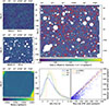 |
Fig. A.1. Left Top:Herschel/SPIRE 250 μm map of the COSMOS field, used in the forward modeling framework of LinSimStack as the data vector d. This corresponds to our z ∼ 0.65 tomographic bin for [CII]-158 μm. Left Middle: Model m from LinSimStack, a linear combination of hit-maps of individual bins, convolved with the 250 μm beam, with the coverage mask of COSMOS2020 applied. Top Right: Residuals d − m not resolved by LinSimStack. We overplot the positions of the brightest 500 COSMOS sources in the Herschel SPIRE Point Source Catalog at 250 μm. Bottom Left: Per-pixel noise in the 250 μm map. Bottom middle: Histograms of the data, LinSimStack fit, and the unresolved residuals, all scaled by the per-pixel noise level after masking. Each is mean-subtracted independently. The residuals are more (standard) Gaussian than the map, with a high-end tail noting the missing sources in the COSMOS2020 catalog. Bottom right: Flux in the map versus in the residuals at the pixel location of sources in the Herschel/SPIRE point source catalog. Also plotted is a linear fit, with each pixel location weighted by the SNR; this encapsulates a measure of how much LinSimStack under-resolves the HSPSC sources. |
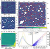 |
Fig. A.2. Same as Figure A.1, but for the Herschel/SPIRE 350 μm map. This corresponds to our z ∼ 1.3 tomographic bin for [CII]-158 μm. |
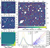 |
Fig. A.3. Same as Figure A.1, but for the Herschel/SPIRE 500 μm map. This corresponds to our z ∼ 2.1 and z ∼ 2.6 tomographic bins for [CII]-158 μm. |
Appendix B: Stacking results
Fig. B.1 shows the stacking outputs from LinSimStack for all of the COSMOS2020 bins, divided by star-forming (SF) versus quiescent (Q) (based on a color selection), redshift (0.01 < z < 6), and stellar mass content (8.5 < log(M/M⊙) < 12). All bins are simultaneously stacked (see Section 3.1), including both the SF (blue and purple resp. for detections and non-detections) and the Q selections (yellow and red resp. for detections and non-detections). We marginalize residuals over all stellar mass bins and SF-Q selection, within a given redshift bin to get our [CII]-158 μm constraints in Fig. 5.
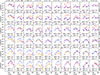 |
Fig. B.1. All results obtained from LinSimStack, while stacking the COMSOS2020 photometric redshifts on 8 maps from the mid-IR to submillimeter. Detections in the star-forming and quiescent selections are denoted by blue and orange crosses, respectively, along with their 1σ uncertainties. For non-detections (measurements consistent with zero), the 3σ upper limits are shown as purple and red arrows for the star-forming and quiescent selection, respectively. Also annotated are the number counts for each selection with the redshift+stellar-mass bins in the photo-z catalog. We do not include stacking estimates for number counts lower than 10; we empirically noted that the SED and bootstrapping errors could not be well constrained within these bins due to low number counts. |
Appendix C: Comparing LinSimStack to SIMSTACK3 from Viero et al. (2022)
Our stacking methodology is similar to SIMSTACK3 from Viero et al. (2022) (V+22), with a crucial change. While SIMSTACK3 formulates the stacking as a non-linear problem and uses a Levenberg–Marquardt algorithm to iteratively converge to a best-fit solution, LinSimStack exploits the linearity of the forward modeling problem to gain an order-of-magnitude speed-up. Notably, our method, unlike SIMSTACK3, does not require a feasible initial guess to converge to the global minima. In Figure C.1, we attempt to replicate stacking results from V+22 (see their Figure 1), by using V+22’s specific choice of binning over COSMOS2020.
Results from LinSimStack (blue) typically agree with SIMSTACK3 results (orange); the RMS of z-scores is ∼1.35, close to 1. Note that the uncertainties plotted and used in the calculation above are just catalog bootstrapping errors (which is all that V+22 use); if we used our more conservative error estimation (Section 3.2), our uncertainties will be  larger (see Fig. 3), resulting in a lower statistic above. We expect LinSimStack is more robust against local extrema in the loss function; we qualitatively note that our stacking estimates trace the continuum better than SIMSTACK3.
 |
Fig. C.1. Replicating Figure 1 from Viero et al. (2022), to compare results from LinSimStack (blue) to SIMSTACK3 (orange). Error bars plotted are from catalog bootstrapping alone (see Section 3.2), to allow a direct comparison with SIMSTACK3/V+22. The RMS of z-scores is ∼1.35, close to the expected unity. We expect our methodology to be more robust against local minima in the loss function. |
Appendix D: Catalog and model predictions for source number counts in COSMOS2020
Tables D.1 and D.2 list number counts in the COSMOS2020 photo-z catalog Weaver et al. (2022) and those obtained from the stellar mass function (SMF) Weaver et al. (2023) model, for the star-forming and quiescent selection of sources, respectively.
Number counts for the star-forming selection of galaxies in the COSMOS2020 photometric redshift catalog, used for simultaneous stacking with LinSimStack.
Same as Table D.1, but for the quiescent selection of galaxies.
All Tables
Estimated bias from contaminating spectral lines within the Herschel/SPIRE broad bandpass for each [CII]-158 μm redshift bin.
Number counts for the star-forming selection of galaxies in the COSMOS2020 photometric redshift catalog, used for simultaneous stacking with LinSimStack.
All Figures
|
Fig. 1. Overview of data used in our analysis. We include transmission curves (left vertical, bottom horizontal axes) for the eight broadband maps used, from Spitzer, Herschel, and SCUBA-2. We overplot the rest-frame wavelengths of selected FIR emission lines, including [CII]-158 μm; these lines are redshifted into the broadband maps. The top horizontal axis labels translate the observer wavelengths into the rest-frame redshift z of a [CII]-158 μm emitter. We trace the z distribution of the COSMOS2020 photometric catalog (in bins of Δz = 0.05), with number counts on the right vertical axis; number counts for the selection of star-forming or quiescent emitters are also shown. Redshifted C+ emission will appear in the SPIRE maps for specific z ranges. Finally, at the top, we demarcate the z-binning used for stacking with LinSimStack; bins at z ∼ 0.65, 1.3, 2.1, and 2.6 were chosen to overlap with the SPIRE bands. |
| In the text | |
|
Fig. 2. Zoom-in on the stacking outputs for the Herschel/SPIRE 250 μm COSMOS map, illustrating our forward modeling LinSimStack methodology. Left to right: 2D vectors for the data d, model m, and the residuals r = d − m. The model m is a linear combination of all beam-convolved hit-maps constructed using the COSMOS2020 photometric catalog. We also plot sources from the Herschel/SPIRE Point Source Catalog (HSPSC) with estimated fluxes in the HSPSC above 30 mJy, which correlate with the residual flux in the 2D vector r (see Section 3.4, Appendix A, the corresponding figures, and the discussion for further details on model incompleteness). |
| In the text | |
|
Fig. 3. Errors in stacked mean intensities estimated via four methods (see Section 3.2). Fractional errors in the stacked fluxes, obtained as outputs of the LinSimStack are color-coded by band. The statistical lower bound is given by the closed-form error formulation, obtained by writing the stacking problem as a linear regression. Bootstrapping the catalog or the pixels captures the additional systematic errors, as it samples different realizations of pixel noise and emitter variance; empirically, the bootstrapping over the catalog (lower left subplot) typically yields the more conservative error estimates. Jack-knifing (JK) provides an estimate of the cosmic variance (CV) at the scale of the map. We conservatively add in, in quadrature, the JK estimate with the maximum of the other three estimates. This effectively lower-bounds our bootstrapping error estimate by the analytical linear formulation limit. Past analyses (Viero et al. 2022, 2013) have only used catalog bootstrapping as the error estimation method. The main subplot above (top-left) compares our final error estimates with those from catalog bootstrapping alone. Our estimates are more conservative by definition and additionally include a measure of CV. |
| In the text | |
|
Fig. 4. Stacked intensity estimates obtained from LinSimStack for individual COSMOS2020 bins, fit with a modified black-body emission continuum SED model. The top panels of each sub-figure show the stacked mean intensities (blue crosses) and corresponding 1σ envelope of the emcee fits (blue) for a subset of the catalog bins; the bottom panels show the signal-to-noise of the fit residuals. The vertical dashed line represents the wavelength cut, λcut, between the two piecewise components of the SED continuum model in Eq. (3) (i.e., the frequency ν0). For a specific z interval, [CII]-158 μm emission is redshifted into a SPIRE band and manifests as excess residual emission over the continuum; these are marked in orange. The SPIRE 500 μm map contains redshifted [CII]-158 μm from the highest two z bins. Different rows and columns correspond to different stellar mass log(M/M⊙) and redshift z cuts; all bins shown here are from the star-forming selection. The labels indicate the number count within a bin in the catalog and as predicted by the stellar mass function (SMF) from Weaver et al. (2023). We conservatively inflate the variance on the [CII]-158 μm residual emission by the reduced chi-squared, χr2, statistic of each SED fit. The bottom row shows residuals obtained by adding over all bins at the same redshift interval, with potential [CII]-158 μm emission again marked in orange. For brevity, we only show stacking within the three highest stellar mass bins (for each redshift bin with potential [CII]-158 μm emission); these are the predominant contributors to the CIB and [CII]-158 μm emission. (See Appendix B for stacking results in all bins.) The bottom row shows the residuals obtained by adding all stellar mass and star-forming plus quiescent bins at a redshift. |
| In the text | |
|
Fig. 5. Measurements of [CII]-158 μm at z ∼ 0.3 − 2.9 compared with [CII]-158 μm-LF estimates in the local universe (Hemmati et al. 2017) and z ∼ 5 (Yan et al. 2020). Also shown are theoretical predictions from C+ evolution models, including Gong et al. (2012) (blue hatches), Padmanabhan (2019) (dotted purple: best model, shaded band: uncertainty), Yang et al. (2022) (dash-dotted green), and Béthermin et al. (2022) (cyan line: De Looze et al. 2014 version; cyan dashed: high SFRD version at high z). Our 3σ upper limits disfavor high-temperature collisional excitation frameworks and best-fit empirical models calibrated to the Pullen et al. (2018), Yang et al. (2019)Planck measurement. The 1σ results are more consistent with SFR-scaling models, which calibrate C+ luminosity to the SFR of sources. Additionally, we show the COBE/FIRAS measurement of the monopole spectrum of the CIB as a function of wavelength, matched to the rest-frame redshift of [CII]-158 μm emission. The [CII]-158 μm contribution is likely no more than a few percent of the total CIB, with the intensity history evolving by less than an order of magnitude across cosmic moon. |
| In the text | |
|
Fig. 6. Population-average [CII]-to-IR luminosity ratios, derived comparing our [CII] constraints with integrated IR luminosity function of Gruppioni et al. (2013). Red limits and pink crosses indicate 3σ upper bounds and 1σ intervals in each redshift bin. Purple bars show the variance-weighted average over all bins (z ∼ 0.33 − 2.9), with dark purple and light purple indicating 1σ and 2σ intervals. We also show the average ratios for local SFGs from [CII] observations from Accurso et al. (2017), and for LIRGs and ULIRGs from Díaz-Santos et al. (2017). |
| In the text | |
|
Fig. 7. Constraints with 3σ upper bounds vs. 95% C.L. bounds from Yang et al. (2019) (a followup of Pullen et al. (2018)) measurement at z ∼ 2.6. No [CII]-158 μm is detected at the previously tentatively reported levels; our best estimates are ∼7.5× lower, with the other 3σ upper bound at z ∼ 2.6 lower than the 95% C.L. interval. Expected 3σ sensitivity limits of two in-development surveys (Pullen et al. 2023; Bracks et al., in prep.) which will measure C+ at high R, are also shown. This tension is discussed further in the text (Section 4). |
| In the text | |
|
Fig. A.1. Left Top:Herschel/SPIRE 250 μm map of the COSMOS field, used in the forward modeling framework of LinSimStack as the data vector d. This corresponds to our z ∼ 0.65 tomographic bin for [CII]-158 μm. Left Middle: Model m from LinSimStack, a linear combination of hit-maps of individual bins, convolved with the 250 μm beam, with the coverage mask of COSMOS2020 applied. Top Right: Residuals d − m not resolved by LinSimStack. We overplot the positions of the brightest 500 COSMOS sources in the Herschel SPIRE Point Source Catalog at 250 μm. Bottom Left: Per-pixel noise in the 250 μm map. Bottom middle: Histograms of the data, LinSimStack fit, and the unresolved residuals, all scaled by the per-pixel noise level after masking. Each is mean-subtracted independently. The residuals are more (standard) Gaussian than the map, with a high-end tail noting the missing sources in the COSMOS2020 catalog. Bottom right: Flux in the map versus in the residuals at the pixel location of sources in the Herschel/SPIRE point source catalog. Also plotted is a linear fit, with each pixel location weighted by the SNR; this encapsulates a measure of how much LinSimStack under-resolves the HSPSC sources. |
| In the text | |
|
Fig. A.2. Same as Figure A.1, but for the Herschel/SPIRE 350 μm map. This corresponds to our z ∼ 1.3 tomographic bin for [CII]-158 μm. |
| In the text | |
|
Fig. A.3. Same as Figure A.1, but for the Herschel/SPIRE 500 μm map. This corresponds to our z ∼ 2.1 and z ∼ 2.6 tomographic bins for [CII]-158 μm. |
| In the text | |
|
Fig. B.1. All results obtained from LinSimStack, while stacking the COMSOS2020 photometric redshifts on 8 maps from the mid-IR to submillimeter. Detections in the star-forming and quiescent selections are denoted by blue and orange crosses, respectively, along with their 1σ uncertainties. For non-detections (measurements consistent with zero), the 3σ upper limits are shown as purple and red arrows for the star-forming and quiescent selection, respectively. Also annotated are the number counts for each selection with the redshift+stellar-mass bins in the photo-z catalog. We do not include stacking estimates for number counts lower than 10; we empirically noted that the SED and bootstrapping errors could not be well constrained within these bins due to low number counts. |
| In the text | |
|
Fig. C.1. Replicating Figure 1 from Viero et al. (2022), to compare results from LinSimStack (blue) to SIMSTACK3 (orange). Error bars plotted are from catalog bootstrapping alone (see Section 3.2), to allow a direct comparison with SIMSTACK3/V+22. The RMS of z-scores is ∼1.35, close to the expected unity. We expect our methodology to be more robust against local minima in the loss function. |
| In the text | |
Current usage metrics show cumulative count of Article Views (full-text article views including HTML views, PDF and ePub downloads, according to the available data) and Abstracts Views on Vision4Press platform.
Data correspond to usage on the plateform after 2015. The current usage metrics is available 48-96 hours after online publication and is updated daily on week days.
Initial download of the metrics may take a while.