| Issue |
A&A
Volume 705, January 2026
|
|
|---|---|---|
| Article Number | A27 | |
| Number of page(s) | 20 | |
| Section | Planets, planetary systems, and small bodies | |
| DOI | https://doi.org/10.1051/0004-6361/202557240 | |
| Published online | 07 January 2026 | |
No TiO detected in the hot-Neptune-desert planet LTT-9779 b in reflected light at high spectral resolution
1
Max-Planck-Institut für Astronomie,
Königstuhl 17,
69117
Heidelberg,
Germany
2
Department of Physics, University of Oxford,
Oxford,
OX1 3RH,
UK
3
NASA Ames Research Center,
Moffett Field,
CA
94035,
USA
4
European Southern Observatory,
Alonso de Córdova 3107,
Vitacura,
Región Metropolitana,
Chile
5
Laboratoire Lagrange, Observatoire de la Côte d’Azur, CNRS, Université Côte d’Azur,
Nice,
France
6
Department of Astronomy & Astrophysics, University of Chicago,
5640 South Ellis Avenue,
Chicago,
IL
60637,
USA
7
Aix Marseille Univ, CNRS, CNES, LAM,
Marseille,
France
8
Instituto de Estudios Astrofísicos, Facultad de Ingeniería y Ciencias, Universidad Diego Portales,
Av. Ejécito 441,
Santiago,
Chile
9
Centro de Astrofísica y Tecnologías Afines (CATA),
Casilla 36-D,
Santiago,
Chile
10
Center for Astrophysics, Harvard & Smithsonian,
60 Garden St,
Cambridge,
MA
02138,
USA
11
Departamento de Astronomía, Universidad de Chile,
Camino el Observatorio 1515,
Las Condes,
Santiago,
Chile
12
Department of Astronomy, University of Michigan,
1085 South University Avenue,
Ann Arbor,
MI
48109,
USA
★ Corresponding author: This email address is being protected from spambots. You need JavaScript enabled to view it.
Received:
15
September
2025
Accepted:
7
November
2025
Abstract
LTT-9779 b is an inhabitant of the hot-Neptune desert and one of only a few planets with a measured high albedo. Characterising the atmosphere of this world is the key to understanding the processes that dominate in reducing the number of short-period intermediatemass planets that create the hot-Neptune desert. We aim to characterise the reflected light of LTT-9779 b at high spectral resolution to break the degeneracy between clouds and atmospheric metallicity. This is key to interpreting its mass-loss history, which might illuminate how it kept its place in the desert. We used the high-resolution cross-correlation spectroscopy technique on four half-nights of ESPRESSO observations in 4-UT mode (16.4 m effective mirror) to constrain the reflected-light spectrum of LTT-9779 b. We did not detect the reflected-light spectrum of LTT-9779 b although these data had the expected sensitivity at the level 100 ppm. Injection tests of the post-eclipse data indicated that TiO should have been detected for a range of different equilibrium chemistry models. Therefore, this non-detection suggests TiO depletion in the western hemisphere, but this conclusion is sensitive to temperature, which affects the chemistry in the upper atmosphere and the reliability of the line list. Additionally, we were able to constrain the top of the western cloud deck to Ptop, western < 10−2∙0 bar and the top of the eastern cloud deck to Ptop, eastern < 10−0∙5 bar, which is consistent with the predicted altitude of MgSiO3 and Mg2SiO4 clouds from JWST NIRISS/SOSS. While we did not detect the reflected-light spectrum of LTT-9779 b, we verified that this technique can be used in practice to characterise the reflected light of exoplanets at high spectral resolution when their spectra contain a sufficient number of deep spectral lines. Therefore, this technique may become an important cornerstone of exoplanet characterisation with the ELT and beyond.
Key words: planets and satellites: atmospheres / planets and satellites: gaseous planets
© The Authors 2026
 Open Access article, published by EDP Sciences, under the terms of the Creative Commons Attribution License (https://creativecommons.org/licenses/by/4.0), which permits unrestricted use, distribution, and reproduction in any medium, provided the original work is properly cited.
This article is published in open access under the Subscribe to Open model.
Open Access funding provided by Max Planck Society.
1 Introduction
Planet LTT-9779 b is a rare example of a mature (age ∼2 Gyr) intermediate-mass (M ~ 29 Me) ultra-short period (P ~ 0.79 d) planet with an atmosphere that currently comprises approximately 9% of the planet mass (Jenkins et al. 2020, see Table 1 for more details). Despite the age of this system, it is possible that is atmosphere is still undergoing mass loss. There is an observed dearth of planets such as LTT-9779 b (e.g. Mazeh et al. 2016), which is often referred to as the hot-Neptune desert. The root cause of the hot-Neptune desert is uncertain, and it might be the result of one or more underlying processes such as photo-evaporative atmospheric loss (Lopez & Fortney 2013; Owen & Wu 2013, 2016, 2017), core-powered mass loss of the atmospheres (Ginzburg et al. 2018; Gupta & Schlichting 2019, 2020, 2021; Gupta et al. 2022), planet migration leading to tidal disruption (Matsakos & Königl 2016; Owen & Lai 2018), and biases in the outcomes of planet formation (Lee & Connors 2021 ; Lee et al. 2022; Nielsen et al. 2025). Additionally, because LTT-9779 b lies close to the inner edge of the hot-Neptune desert, it might currently or in the past have been subject to Roche-lobe overflow (Jackson et al. 2017; Koskinen et al. 2022). If any or a combination of these processes shaped the desert, then some property of the atmosphere of LTT-9779 b, its space environment, system age, and/or history must have caused it to keep its current place there. By studying this system, we learn more about the processes that allow its atmosphere to survive and how they shape the hot-Neptune desert.
This system has already been the focus of numerous studies that showed it to have a number of unusual properties. Fernandez et al. (2023) used x-ray multi-mirror mission (XMM-Newton) observations to show that the extreme ultraviolet radiation output of LTT-9779 was much lower than is typical. This would allow LTT-9779 b to retain an atmosphere to this day if it started with an envelope fraction greater than 10%, although it would still be undergoing photo-evaporation. Edwards et al. (2023), Vissapragada et al. (2024), and Radica et al. (2024) did not detect signatures of mass loss in the 1.083 μm helium line using transit observations taken with the wide field camera 3 on Hubble (WFC3/Hubble), the warm infrared echelle spectrograph to realize extreme dispersion and sensitivity on Magellan II (WINERED/Magellan II), and the near infrared imager and slitless spectrograph on the James Webb space telescope (NIRISS/JWST), respectively. This either limits the mass-loss rate to below the upper limit predicted by Fernandez et al. (2023) or implies that this line is not excited. Alternatively, Radica et al. (2024) posited that the clouds might suppress atmospheric escape by lowering the temperature of the atmosphere. To determine whether LTT-9779 b is undergoing mass loss and measure the mass loss rate, more information on its atmosphere is needed.
Several studies have measured the atmospheric metallicity of LTT-9779b (Crossfield et al. 2020; Hoyer et al. 2023; Edwards et al. 2023; Radica et al. 2024; Coulombe et al. 2025; Reyes et al. 2025; Zhou et al. 2025; Ashtari et al. 2025), but the constraints are weak, and the results are not fully consistent with each other. For example, Coulombe et al. (2025) used NIRISS/JWST in single object slitless spectroscopy mode (JWST NIRISS/SOSS) to obtain a reflected-light phase curve and suggested that the metallicity in the atmosphere is lower than 30 times solar, while Crossfield et al. (2020) used a 4.5 μm Spitzer phase curve to suggest instead that the metallicity was greater than 30 times solar. Hoyer et al. (2023), Radica et al. (2024), Reyes et al. (2025), and Ashtari et al. (2025) all favoured high metallicities, with the first requiring greater than 400 times solar metallicity to explain the optical albedo, the next two requiring metallicities of 20-850 times and greater than 180 times solar, respectively, to explain the flat transmission spectrum, and the last suggesting greater than 500 times solar based on the phase curve observed by the Near Infrared Spectrograph (NIRSpec) on JWST in G395H mode. In contrast, Edwards et al. (2023) presented WFC3/Hubble transit observations that suggested a metallicity lower than 0.1 times solar, but these data were reanalysed by Zhou et al. (2025), who found similar values until they included the JWST NIRISS/SOSS data from Radica et al. (2024), which increased the metallicity to 275 times solar. The lack of strong consistent constraints on the metallicity of LTT-9779 b is a strong barrier against understanding the atmosphere of this world, and based on this, its place in the desert through its link with the planet formation history and mass loss (e.g. Fortney et al. 2013; Lee & Chiang 2016; Owen & Wu 2017; Louca & Miguel 2025).
In additional to the metallicity, several studies also investigated the abundances of individual atmospheric species. Dragomir et al. (2020) showed Spitzer secondary-eclipse data that strongly favoured models containing CO or CO2, while Coulombe et al. (2025) used JWST NIRISS/SOSS phase curves to constrain the water abundance. Edwards et al. (2023) and Zhou et al. (2025) both studied the same WFC3/Hubble transits, but were unable to robustly constrain the atmospheric species and obtained inconsistent results. Furthermore, while hot Jupiters with a similar equilibrium temperature as LTT-9779 b tend to have inversions (Parmentier et al. 2016), Spitzer and JWST observations indicate that the dayside atmosphere has a non-inverted temperature profile (Dragomir et al. 2020; Coulombe et al. 2025). This can imply a lack of absorbers such as VO and TiO at high altitudes. This is an indirect measurement, however, and additional data are required to confirm the lack of these species in the upper atmosphere of LTT-9779 b.
The difficulty of constraining the metallicity and detecting the spectral features of single species is likely due to the clouds in the atmosphere. They essentially hide the lower atmosphere layers and can reduce the size of the spectral features, which makes them harder to detect and constrain. The altitude of the cloud deck determines how much of the atmosphere can be obscured by the clouds, and in this way, how much the spectral features are reduced in size. It is difficult to constrain the altitude of the cloud deck, however, because spectral feature can also be reduced in size if the metallicity is lower, which causes degeneracies between these two parameters.
LTT-9779 b has one more unusual trait: It is one of only a handful known highly reflective worlds (Hoyer et al. 2023; Coulombe et al. 2025; Saha et al. 2025). JWST NIRISS/SOSS phase curves have shown this reflection to vary spatially between the western limb (geometric albedo (Ag) of 0.8) and the eastern limb (Ag = 0.4 (Coulombe et al. 2025). Coulombe et al. (2025) showed that their data were consistent with Mg2SiO4 and/or MgSiO3 clouds that are primarily present on the western hemisphere of the planet. This spatial distribution is consistent with common trends seen in hot Jupiters, where the cooler temperatures on the evening limb cause cloud formation (Fu et al. 2025). Furthermore, the non-detection of the planet eclipse with the ultraviolet and visual echelle spectrograph (UVES) on the VLT also suggests Mg2SiO4 and/or MgSiO3 clouds (Radica et al. 2025). The altitude of these clouds remains unconstrained (Radica et al. 2025; Coulombe et al. 2025).
The reflected light of an exoplanet is comprised of the light of its host star, which has been scattered by the exoplanet, and its atmosphere in the direction of the observer. Thus, the reflected stellar light becomes imprinted with absorption features from the dayside atmosphere of the exoplanet. When the exoplanet has a highly reflective cloud deck, the spectral lines are formed primarily by the atmosphere above the clouds. The clouds themselves do not produce spectral lines in this wavelength range, but change the continuum of the spectrum. This means that the depth of the spectral features, assuming the reflectivity of the clouds is fixed, is dependent both on the abundance of a given species in the upper atmosphere and on the altitude of the cloud deck. Current data are not sensitive enough to break the degeneracy between metallicity and cloud deck altitude. At high spectral resolution, however, this degeneracy is broken because the altitude of the cloud deck alters the shape of the spectral lines. Gandhi et al. (2020) reported examples of the breaking of this degeneracy for transmission spectra, and Fig. 1 shows the same for reflection spectra based on the models from Sect. 5.2.2.
High-resolution cross-correlation spectroscopy (HRCCS Snellen et al. 2010) is a well-established technique for obtaining and characterising high-resolution exoplanet spectra. The technique has predominantly been used on the transmission and emission spectra of exoplanets (see Birkby 2018; Snellen 2025). Attempts have been made to study reflection spectra with this technique (Martins et al. 2015; Hoeijmakers et al. 2018b; Scandariato et al. 2021; Spring et al. 2022), but no robust detections were obtained. Martins et al. (2015) claimed a detection of the reflected light of 51 Pegasi b, but Scandariato et al. (2021) and Spring et al. (2022) later showed this to be an unfortunate false positive. The lack of a successful detection of the reflected light of an exoplanet at high spectral resolution has so far been attributed to the low albedos of the previously targeted exoplanets. LTT-9779b is known to have a high albedo (Hoyer et al. 2023; Coulombe et al. 2025; Saha et al. 2025) which makes it a good candidate for this technique.
Beyond learning more about the atmosphere and clouds of LTT-9779 b, it is of wider importance to the future of exoplanet characterisation to demonstrate the HRCCS technique in reflected light on LTT-9779 b. Earth-like planets have low transit probabilities and are relatively cool, with little thermal emission in the optical and near-infrared. Therefore, the reflected light of these worlds will form an important part of the characterisation of their atmospheres. For the Extremely Large Telescope (ELT), this characterisation will largely focus on the use of high-resolution techniques such as HRCCS and the related molecule-mapping technique (Snellen et al. 2015; Hoeijmakers et al. 2018a).
We aim to demonstrate the HRCCS technique on the reflected light of LTT-9779 b. In Sect. 2 we discuss the observations, and in Sect. 3 we refit the orbit of LTT-9779 b using these data. In Sect. 4 we discuss the HRCCS data reduction, and the reduced data are analysed in Sect. 5. In Sect. 6 we discuss our results. Finally, we discuss the atmospheric constraints imposed by these data and highlight future directions in Sect. 7. We conclude in Sect. 8.
Summary of the LTT-9779 system.
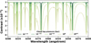 |
Fig. 1 Spectrum of a hydrogen-helium atmosphere with a uniform volume-mixing ratio of Fe of 0.0001 (see Sect. 5.2.2). Each line represents a model with a grey cloud deck at a different altitude. This is represented by the cloud top pressure. |
2 Observations
The HRCCS technique requires a time-series of high-resolution spectra with a high signal-to-noise ratio (S/N) of the combined star-planet system so that the changing Doppler shift of the planet can be used to isolate its spectrum. We observed the host star LTT-9779 (G7V, V = 9.76 mag) for four half-nights, each covering before, during1, and after secondary eclipse of LTT-9779 b, using the echelle spectrograph for rocky exoplanets and stable spectroscopic observations (ESPRESSO; Pepe et al. 2021) on the Very Large Telescope (VLT) at Paranal Observatory, Chile (PI: Vaughan; Program ID: 112.25T7). This phase coverage is possible due to the short approximately 19-hour orbital period, which allowed around 25% of the orbit to be observed on each half-night.
These observations used the ESPRESSO 4-UT mode. In this mode, the ESPRESSO instrument is fed light from all four of the VLT unit telescopes (UT) simultaneously. The light reaches the instrument in a bundle of four fibres, and the combined light is projected onto the spectrograph. ESPRESSO was designed to operate in the slit-limited regime of resolution, which means the wider fibre bundle results in a lower spectral resolution compared with the available 1-UT modes. However, the S/N of the resulting spectrum is significantly higher primarily due to the larger collecting area2 provided by using multiple telescopes. Overall, the S/N of a spectrum increases by a factor of approximately 2.7 when 4-UT mode is used over 1-UT mode. This observing mode has been used for exoplanet transit characterisation in the past (Borsa et al. 2021; Seidel et al. 2025; Prinoth et al. 2025) but not to study an exoplanet in reflected light. As part of the observing proposal, we used a modified version of the ESPRESSO exposure time calculator to simulate these observations at the appropriate spectral resolution. These simulated observations contained the tellurics, seeing and airmass trends as well as the appropriate read, dark, and photon noise. We modelled the spectrum of LTT-9779 b assuming chemical equilibrium and so the spectrum contained a large number of deep TiO lines. When the simulated observations were analysed, using the same techniques as would be applied to real data, the signal of the planet spectrum was recovered at a S/N of approximately ten.
In 4-UT mode, ESPRESSO covers a simultaneous wavelength range of 380 nm to 788 nm at a spectral resolution of R ~ 70 000 (Pepe et al. 2021). Therefore the instrumental broadening (or resolution element) is approximately 4.3 km s−1 and the atmospheric absorption lines in the planet’s spectrum3 are dominated by this instrumental broadening since the planetary spin, assuming tidal locking, results in a broadening of only around 2.7kms−1. We used an integration time of 300 s during the first night of observations due to the reduced seeing conditions, which caused less light to enter the fibre. This integration time led to a Doppler smearing of approximately 5.3 km s−1 for phases outside of the secondary eclipse. This is slightly larger than the resolution element, but we elected to favour obtaining a higher S/N in the continuum. Subsequent nights experienced better seeing so an integration time of 200 s was used instead to avoid saturation. The Doppler smearing in these observations is less than 4.3 km s−1 for the observed fraction of the orbit. The third night of observation was halted due to precipitation at the VLT site and was not restarted. A summary of the observations is given in Table 2.
The spectra were extracted from the raw data using ESOReflex v2.11.5 and ESPRESSO pipeline v3.1.0. This pipeline performs a number of standard calibrations such as bias correction, flat fielding, wavelength calibration and background subtraction. The spectra are extracted into the barycentric rest frame and into either a single combined spectrum or into their individual spectral orders. We chose to use the latter to reduce the amount of preprocessing which can alter the systematics in the data. In addition to extracting the spectra, the ESPRESSO pipeline also computed the cross-correlation function of the host star for each observation using a binary mask (G9) selected based on the stellar type of LTT-9779 (G7V). This is then used to calculate a precise stellar radial velocity for each observation.
Summary of the LTT-9779 eclipse observations.
3 Refitting the orbit of LTT-9779 b
HRCCS usually requires the cross-correlation of each exposure to be stacked in the planetary rest frame so that the signal of the spectrum of the planet can be confidently detected. This requires an accurate planetary ephemeris to predict the orbital phase, and thus the velocity of the planet. The error in the orbital phase prediction comes primarily from the uncertainty in the orbital period, which can result in a large discrepancy between predictions and the true orbital phase if the planet has completed many orbits since the measurement. There are three ephemerides for LTT-9779 b; the discovery ephemeris from Jenkins et al. (2020) and two updates (Edwards et al. 2023; Kokori et al. 2023). The Jenkins et al. (2020) ephemeris has a 0.8 s error on the orbital period which propagates to an uncertainty in the orbital phase of 0.0054 after one Earth year or ∼0.028 during the epochs of our ESPRESSO observations. It is thus unsuitable for our analysis. The other two ephemerides (Edwards et al. 2023; Kokori et al. 2023) have errors on the orbital period of 0.012 s and 0.024 s respectively and are also more recent, meaning that fewer orbits have occurred since they were measured. Therefore the uncertainty in the orbital phase for both ephemerides is less than 0.001 when propagated to our observation epochs and the predictions are within the one sigma errors of each other. This corresponds to an error in the velocity of the planet of approximately 0.7 km s−1 at secondary eclipse. At R = 70000, the velocity resolution is 4.3 km s−1 or approximately six times greater than the error which is sufficiently accurate for our analysis.
However, with the precise stellar radial velocities measured by the ESOReflex pipeline and high temporal cadence of these observations, it is possible to constrain parameters such as the orbital eccentricity of LTT-9779 b. A non-zero eccentricity could be an indication of high-eccentricity migration (Matsakos & Königl 2016; Owen & Lai 2018), one of the processes that might form the hot-Neptune desert. A small eccentricity can also raise the internal temperature via tidal heating (Leconte et al. 2010) which would affect the interpretation of atmospheric parameters.
Using only the radial velocities from these observations does not constrain the orbit of the planet due to the limited phase coverage. We created a more complete radial velocity curve by including the radial velocities from three nights of 1-UT ESPRESSO transit observations (PI: Jenkins, Program ID:103.2028 and PI: Ramirez Reyes, Program ID:108.22FQ) as well as the tabulated radial velocities from the high accuracy radial velocity planet searcher (HARPS)4 presented in Jenkins et al. (2020). Additionally, the short cadence (<2 mins) transiting exoplanet survey satellite (TESS) light curves are extracted with lightkurve python package (Lightkurve Collaboration 2018) and fit simultaneously with these data.
The orbit is modelled using the exoplanet python package (Foreman-Mackey et al. 2021) and we used the Bayesian inference package pymc3 (Salvatier et al. 2016) to compute the best fit. We selected the pymc3 no-u-turn sampler sampler to evaluate the posteriors of each fit which we used to calculate the uncertainties. We chose not to use nested sampling as the results can be less robust in this instance. We preformed two fits, one with the eccentricity fixed to zero and a second where eccentricity is a free parameter, the results of which are shown in Table 3. Both orbital fits assumed that LTT-9779 b is the only planet in the system.
The eccentric orbit fit, which favours a non-zero eccentricity e = 0.010 ± 0.002, has a slightly lower reducedχ2 indicating it is a better fit to these data. However, the Bayesian Information Criterion strongly favours the circular fit. This is because the improvement in the fit does not warrant the additional complexity that comes with adding the eccentricity as an additional parameter. Since the fit is not favoured, further radial velocity observations would be needed to robustly constrain the eccentricity of this system beyond putting a three sigma upper limit of e < 0.016. Fig. 2 shows the best fit circular orbit on the phase folded radial velocities and light curve. In this work, we used the circular orbit ephemeris to calculate the orbital phases of LTT-9779 b covered by the observations shown in Fig. 3.
4 Removing contaminating spectra
In the time-series of observations, the position of the planetary spectral lines changes significantly due to the orbital motion of the planet, but the stellar lines and the telluric lines remain quasi-stationary in wavelength. The HRCCS technique isolates the spectrum of the planet by removing the quasi-stationary trends created by the stellar and telluric lines. Because the spectrum of LTT-9779 b is buried in the stellar spectrum at approximately the 100ppm level (Hoyer et al. 2023; Coulombe et al. 2025; Radica et al. 2025; Saha et al. 2025), the data reduction must remove the contaminating spectra to at least this degree. In this section we discuss the standard techniques employed to achieve this level of cleaning.
Previously derived orbit parameters for LTT-9779 b along with those derived in this work.
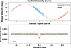 |
Fig. 2 Top panel: phase-folded radial velocity curve comprised of radial velocity measurements from this work (ESPRESSO eclipse), ESPRESSO transit observations, and HARPS. The vertical extent of each point represents the error. For the radial velocities to appear as a continuous curve, the systemic velocity and the fitted instrumental offset were subtracted. Bottom panel: phase-folded short-cadence TESS light curve (light points). The darker points show a binned version of the curve. In both panels, the best-fit curve for a circular orbit is shown (orange). |
 |
Fig. 3 Phases of LTT-9779 b, assuming the ephemeris from the circular orbit fit in Table 3, covered by these observations. Each circle represents an exposure, and the shaded area indicates the secondary eclipse of the planet. The gaps in the observations taken on night 1 were due to technical difficulties, and the observations in night 3 were halted early due to precipitation. |
4.1 Outlier removal
The first step of this process is to remove the outliers missed by the ESPRESSO pipeline. The outlier removal was applied to the spectral time-series of each order and each night separately in the barycentric rest frame used by the ESPRESSO pipeline. Using the barycentric rest frame for this part of the reduction minimised the need to interpolate the outliers which improves their removal. To remove the outliers, each spectrum in the timeseries of a given spectral order was first continuum normalised using a fourth order polynomial fit that excludes data more than ten standard deviations from the mean. Next, the blob detection algorithm described in Kong et al. (2013) was run. It flagged outliers with a threshold of 4σ and replaced them by interpolating the surrounding non-flagged data. The data used are both adjacent in wavelength and time, using the spectra taken before and after the outlier. Since the spectra are in the barycentric rest frame, both the stellar and telluric lines will not be stationary in wavelength. However, the Doppler shift between adjacent spectra was significantly below the instrumental resolution and thus this had minimal impact on the outlier removal. We ran the algorithm either five times or until no more outliers are removed, which ever came first. This removed the worst outliers but a visual inspection of the data revealed some had been missed. To identify these too, we transformed to the stellar rest frame and removed the median spectrum of the observations taken during secondary eclipse5 before restoring the data to the barycentric rest frame. This allowed the blob detection algorithm to identify and replace the remaining outliers using a threshold of 2.5σ. Finally, the median spectrum was added back into the data and the continuum restored. The reason for this last step is discussed in Sect. 5.6.
4.2 Removing stellar and telluric spectra
To remove the contaminating stellar and telluric spectra, we performed the following on the spectral time-series of each order and each night separately since they might have different systematics. The spectra start in the barycentric rest frame but were converted into the stellar rest frame during this part of the data reduction. An example of these processes is shown in Fig. 4.
The first step is to correct for the continuum where variations in flux are primarily due to atmosphere of the Earth. This was achieved by dividing each spectrum in the time-series by a smoothed version of itself which was computed by convolving it with a box function 255 pixels wide. This width was chosen via trial and error and visually appears to work best. Next, each spectrum in the time series was interpolated from the barycentric frame into the stellar rest frame. Once in this new frame, the median spectrum of the spectra taken during secondary eclipse5 was subtracted from each observation.
While this removes the majority of the contamination, clear residuals from many spectral lines remain in the time-series as seen in the third panel of Fig. 4. The dominant source of contamination in these data are the spectral lines from the star. Because the effect of the tellurics is weaker and they are primarily produced by species in which we are not interested, we chose to use sysrem over telluric fitting models such as molecfit (Smette et al. 2015; Kausch et al. 2015) to remove this contamination. The fourth to sixth panels of Fig. 4 show several iterations of this algorithm removing the remaining residuals. Since the sysrem algorithm focuses on agnostically removing stationary trends from the data, it is possible that it might remove some or all of the planetary spectrum. This can be the case if too many sysrem iterations are used, if the spectral lines change the Doppler shift too slowly or are significantly Doppler smeared or rotationally broadened. These observations were designed such that the change in Doppler shift between observations should be large enough to avoid causing a significant effect, and the atmospheric spectral lines of the planet are not expected to be significantly Doppler smeared6 or rotationally broadened (2.7 km s−1; see Sect. 2). Some spectral lines may become intrinsically broadened when the species abundance is high or the cloud deck is low. Injection recovery tests can be used to verify if this broadening is impacting the recovery of the spectrum of the planet. Therefore only the number of sysrem iterations might cause a problem. To select the number of sysrem iterations, we followed a process similar to that described in (Spring et al. in prep). The sysrem algorithm (Tamuz et al. 2005) was run a total of ten times on the spectral time-series of each order with the result for each iteration saved. These were then used to choose the number of sysrem iterations. This was done by measuring the point at which the change in standard deviation of the reduced spectra in the time-series between iterations drops to within one standard deviation of the changes between the last four iterations. If there was no change in the standard deviation in the last four iterations, then the last iteration that removed some component was used instead. This is demonstrated in the last panel of Fig. 4.
Successful recovery of injected models, for example in Fig. 8, indicates that the sysrem algorithm does not destroy the spectrum of the planet, although it may still damage it. Ideally, one would use physics based models for the stellar spectrum like those used for the tellurics. Unfortunately, this is not currently possible and algorithms like sysrem are the main alternative. In Sect. 6 we used injection recovery tests to study the constraining power of our data to different model atmospheres. Since the injected spectra undergo the same data reduction, they will be similarly damaged and so these are a realistic estimate for the sensitivity of our data given the current data reduction.
Finally, to remove any residual slowly changing continuum, which can cause artefacts in the later analysis, each spectrum in the time-series was high pass filtered. This was achieved by subtracting a smoothed version of each spectrum computed by convolving the spectrum with a box function 255 pixels wide. Again, this width was chosen via trial and error.
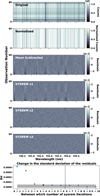 |
Fig. 4 Schematic of the data reduction process for the spectral time series of order 76 in night 2. Each of the six top panels shows the time series of spectra. Each row represents one spectrum in the series. Top panel: original spectra. Second panel from the top: spectral time series after continuum normalisation. Third panel from the top: spectral time series after the mean spectrum was subtracted. Panels 4-6 from the top: Spectral time series after one, two, and three sysrem iterations were run on the time series. Bottom panel: difference in the standard deviation of the residuals between consecutive sysrem iterations as a function of the number of sysrem components. The shaded region highlights the one-sigma deviation in the last four points (to the right of the dashed line), and the black dot indicates the chosen number of iterations (the smaller number), as described in the text. |
5 Recovering the spectrum of the planet
While the data reduction presented in Sect. 4 was able to successfully remove the stellar and telluric spectra, it was unable to remove the photon noise from the star. This noise prevents the spectrum of the planet from being measured directly, even when all observations are combined. However it is still possible to extract useful information on the embedded planets spectrum by matching it to model spectra using the likelihood method. In this work, we used the likelihood metric presented in Brogi & Line (2019).
5.1 The likelihood method
This method compares a Doppler-shifted model spectrum, g(λn - λs), to the reduced spectrum of a single observation and spectral order, fobs,order(λn ) using the following likelihood metric:
![Mathematical equation: \text{log}(L) = -\frac{N}{2} \text{log}[s_f^2 -2R(s) + s_g^2],](/articles/aa/full_html/2026/01/aa57240-25/aa57240-25-eq7.png) (1)
(1)
where s represents the Doppler shift of the model. In this metric, s 2 is the variance of the data, and  is the variance of the Doppler-shifted model,
 (2)
(2)
where g(λn - λs) was interpolated to the same wavelength grid as the observations, so that the sum in both cases is over the pixels, n, in the reduced spectrum.
The central term in the likelihood, R(S ), is the crosscovariance of the data and Doppler-shifted model,
 (3)
(3)
Another standard metric used in HRCCS analyses is the cross-correlation coefficient, C(s), which is related to the cross-covariance via
 (4)
(4)
Both R(s) and C(s) increase when the model is at the right Doppler shift and has spectral lines that match the spectrum of the planet. This leads to an increase in the likelihood, L.
5.2 Generation of the model spectra
In the likelihood framework, we need model spectra to compare to the embedded planet spectrum. Reflection spectra are formed of a reflected version of the stellar spectrum modulated by the wavelength-dependent albedo of the planet. The reflected stellar spectrum is not identical to that which we observe from the star as it experiences a different degree of rotational broadening. This is because, while we view the star rotating with its own rotation period, when viewed from the planet the star appears to be rotating with a combination of the stellar rotation period and the orbital period of the planet. We used Eq. (6) in Spring et al. (2022) to compute the rotational broadening of the reflected stellar spectrum for LTT-9779 b. This yielded a broadening of νref ~ 60kms−1. Therefore, the spectrum of LTT-9779 b will not contain any deep stellar spectral lines and we modelled the stellar spectrum as a continuum. To model the modulation of the reflected stellar spectrum caused by the atmosphere of LTT-9779 b, we used the planetary intensity code for atmospheric scattering observations (PICASO) (Batalha et al. 2019) to compute the planet-star contrast ratio. The atmospheric spectral lines are broadened only by the planetary spin. Assuming tidal locking, this results in a broadening of approximately 2.7 km s−1 which is below the instrument resolution of 4.3 km s−1 and so it was neglected when computing the planet-star contrast ratio. The model of the planetary spectrum was then created by multiplying the modelled stellar spectrum with the generated planet-star contrast ratio.
Our ESPRESSO spectra have R ~ 70000 but PICASO needs opacities several times this resolution to accurately reproduce the spectrum. We elected to use opacities with R ~ 500 000 which are listed in Table A.1. Since the data reduction used a high pass filter, the same filtering must be applied to the models so they can match the real embedded spectrum. We achieved this high pass filtering by subtracting a R = 2000 version of the model spectrum from the full R = 70 000 version. This lower resolution was chosen so that the model spectrum would be smoothed by a filter of similar width to the data (see Sect. 4).
To generate the planet-star contrast ratio, PICASO requires the atmospheric temperature profile to be specified along with the volume-mixing ratios (VMR) of the species in the atmosphere and a model of the clouds. The parameters of all the models used in this work are summarised in Table 4 and discussed in details in the following sections.
5.2.1 Spectral models based on JWST NIRISS/SOSS observations
We used the information provided by previous JWST NIRISS/SOSS observations to construct high spectral resolution model spectra. Examples of the temperature profile, species VMRs and cloud profile used by PICASO to compute these self-consistent model spectra are shown in Fig. A.1 and summarised in Table 4.
We computed three sets of self-consistent model spectra, each for a different segment of the planetary dayside. These are eastern dayside, central dayside (dayside), and western dayside, as defined in Coulombe et al. (2025). Each segment has a different temperature profile for which we used the mean measured from JWST NIRISS/SOSS phase curve observations (Coulombe 2025, shown here in Fig. A.1; T.1 in Table 4). There is a large uncertainty in the temperature profile at low pressures (lower than 10−6 bar) as the JWST NIRISS/SOSS phase curve data are not particularly sensitive to this region of the atmosphere. Therefore, the low-pressure part of the temperature profile has tended towards the centre of the priors used by Coulombe et al. (2025), which results in a hot upper atmosphere. To explore how much our results might change if the upper atmosphere were cooler, as is suggested by the lack of evidence of a thermal inversion (Dragomir et al. 2020), we also created a similar set of models where the temperature profile was made isothermal above 10−5 bar (T.2 in Table 4 and shown in A.1). This resulted in a total of six different temperature profiles, two for each of the three atmospheric segments.
For all six temperature profiles we assumed equilibrium chemistry and computed the VMRs using easychem (Lei & Mollière 2025) for a range of metallicities from 0.1 times solar to 1000 times solar (Ch. 1 in Table 4). The VMRs computed for the 10 times solar metallicity model are shown in Fig. A.1. As discussed in Sect. 1, it is currently uncertain if TiO and VO are present at their equilibrium abundances or if they are depleted. We therefore created variants of these models with the VMR of TiO set to zero (Ch. 2 in Table 4) and with the VMRs of TiO and VO set to zero (Ch. 3 in Table 4) for the same range of metal-licities and for all six temperature profiles. The VMR profiles of some species do differ significantly between the original (T.1) and modified (T.2) temperature profiles as a result of changes in the reaction rates modelled within the easychem chemical network, including notably the profiles of TiO and VO.
Previous works have favoured the presence of Mg2SiO4 and MgSiO3 clouds over those of other types (Hoyer et al. 2023; Radica et al. 2024; Coulombe et al. 2025; Radica et al. 2025). To model these clouds, we used the virga module (Batalha et al. 2025) which implements the Ackerman & Marley (2001) cloud model to compute the extinction and scattering parameters for a set of condensates based on the vertical mixing, kzz, and sedimentation efficiency, fsed. This method is similar to that used in Saha et al. (2025). We used virga to specify appropriate parameters for only Mg2SiO4 and MgSiO3 clouds (Scott & Duley 1996) for each segment assuming kzz = 109, fsed = 1 and that the particle sizes follow a log normal distribution with σ = 2. These parameters are consistent with Radica et al. (2025). The optical depth profile of the combined Mg2SiO4 and MgSiO3 clouds are shown in Fig. A.1 where the top of the clouds are at an altitude of approximately 10−4 bar for the western dayside and dayside models and 10−1.5 bar for the eastern dayside model. We note that the vertical extent and height of these clouds can be changed by varying kzz, fsed or the temperature profile. The altitude of the clouds are not strongly constrained with the JWST NIRISS/SOSS data as the uncertainty in the intersect point between the temperature profile and the cloud species condensation curve that spans a large fraction of the atmosphere (see Fig. A.1). Given the complex way the resulting cloud model is influenced by the input parameters, we elected to use the simpler models described in Sect. 5.2.2 for exploring different cloud scenarios and kept the cloud model fixed for the self-consistent models. Additionally, since the modified temperature profile does not significantly alter the cloud profile, we opted to use the same cloud model for both the original (T.1) and modified (T.2) temperature profiles.
Fig. 5 shows an example self-consistent model spectrum for each segment of the planetary dayside for the original temperature profile (T.1) and 10 times solar metallicity. Each panel shows two versions of the spectra, one with all chemical species (Ch.1) and one with TiO removed (Ch.2). From this, it is clear that TiO causes a large number of the spectral lines. This figure includes the contrast ratio and its error from Fig. 3 of Coulombe et al. (2025) which we reproduced using Coulombe (2025). This demonstrates that these spectra are largely consistent with these previously measured values.
Summary of the inputs to the model spectra.
5.2.2 Free-chemistry single-species models
The self-consistent models assume equilibrium chemistry, but it is uncertain which species are present at high altitudes. Dragomir et al. (2020) found a non-inverted temperature profile which might suggest a lack of TiO and VO at high altitudes and Zhou et al. (2025) suggested that the modelling difficulty they encountered may be the result of some form of disequilibrium chemistry. Disequilibrium chemistry has been seen in giant planet atmospheres before (e.g. Fortney et al. 2020; Sing et al. 2024) so it is possible that this atmosphere might not be in equilibrium. Thus we created sets of single-species model spectra to agnostically search for the presence of individual species, while recognising that the detection strength of such models will be lower that for multi-species models due to the loss of signal caused by excluding the spectral lines of other species. Table 4 summarises the inputs for these the models.
In reflected light, the temperature profile influences the spectrum primarily by setting the chemical equilibrium and condensation points for clouds. However, if both the VMRs and cloud properties are set independently of the temperature profile then the spectrum is not strongly influenced by its parametrisation as the opacities are not strongly temperature dependent. Therefore, for simplicity, we assumed an isothermal temperature profile set to 1800 K and set the VMRs and cloud properties independently.
For the chemical composition, we assumed a hydrogenhelium dominated atmosphere with a trace amount of a single additional species. We chose TiO, VO, Fe, MgH, FeH, H2O and AlH because these species have a large number of spectral lines in the ESPRESSO wavelength range and produce spectral features at feasible abundances. Therefore these represent the best chance for individual detection. The VMR of the trace species is assumed to be constant within the atmosphere and Table 4 summaries the values assumed for each species.
Next, we modelled a single grey cloud deck with a free choice of the altitude, vertical extent, optical depth, asymmetry parameter and single scatter albedo. We assumed a fixed vertical extent of one order of magnitude in pressure and an optical depth equal to ten. The single scatter albedo, ω0 and asymmetry parameter g0 were set such that the continuum matches the pre- and post-eclipse contrast measure by JWST NIRISS/SOSS (Coulombe 2025). That is ω0 = 0.885, g0 = 0.0 for pre-eclipse (C.1 in Table 4) and ω0 = 0.995, g0 = 0.0 for post-eclipse (C.2 in Table 4). This created two sets of single-species models for each species, one for each side of the eclipse. The altitude of the top of the cloud deck was varied in steps of an half order of magnitude in pressure ranging from 100.5 to 10−5 bar.
For each species we created a grid of models that vary the VMR of that species and the height of the cloud deck. The spectral lines shapes of the trace species vary and can be used to identify the presence of a given species in our data.
 |
Fig. 5 High spectral resolution (R = 70000) models computed using the eastern dayside, dayside, and western dayside mean temperature profiles from Coulombe et al. (2025, T.1) assuming 10 times solar metallicity. Each panel shows two spectra, one spectrum that assumes equilibrium chemistry for all species (Ch. 1,) and another that removes TiO from the atmosphere (Ch. 2). The contrast ratio measured by Coulombe et al. (2025, see Fig. 3 of their work) for each segment is shown as the dashed line, and the shaded region indicates the one-sigma errors. |
5.3 Combining all the data
The likelihood shown in Eq. (1) of Sect. 5.1 and the crosscorrelation coefficient in Eq. (4) were computed for a range of model Doppler shifts from –500 to 500 km s−1 in steps of 0.8 km s−1 on the reduced data of each observation and spectral order separately. This step size was chosen as it is approximately equivalent to the velocity spacing of each pixel in the spectrum. This is smaller than the resolution element, 4.3kms−1, as ESPRESSO over-samples the spectrum such that instrumental resolution is equivalent to 5.5 pixels on the detector. The spectrum of the planet is too faint to show a statistically significant increase in the likelihood or cross-correlation coefficients for each observation and order in isolation. To identify the spectrum, all the orders and observations must be combined.
The combination process is the same for the likelihood and cross-correlation values, but for clarity, only the likelihood values are mentioned in the following explanation. First, the likelihoods of each order were summed resulting in one likelihood value for each observation and model Doppler shift. Combining the observations is more complicated as the velocity of the planet is changing and the spectrum of the planet itself is changing as evidenced by differences seen in the eastern dayside, dayside, and western dayside models shown in Fig. 5. To account for the changing spectrum, the observations were split based on the orbital phases they cover. To account for the orbital motion during the selected observations, the likelihood values were summed along a variety of orbital paths defined by
 (5)
(5)
where φ is the a priori known phase of the orbit and the systemic velocity, Vsys, and orbital velocity, Kp, both range from –500 to 500 km s−1 in steps of 0.8kms−1.
This process created a Vsys-Kp map, a 2D colour map indicating how the sum of either the likelihoods or cross-correlation coefficients varies when the data are combined assuming different orbits for the planet. Since the presence of the spectrum of the planet creates an increase in the likelihood and cross-correlation coefficient, the sum will be higher when all these small increases are summed together using the correct orbit. This leads to a peak in the Vsys -Kp map at the location where the systemic and orbital velocities match that of the planet. This will not be the only peak in the map as noise can cause fluctuations in the sum creating a series of peaks and troughs over the whole map. These might also show correlated structure if residuals from the tel-lurics or the stellar spectrum remain in the data. Alternatively this structure might come from the planet itself if the signal is strong and the autocorrelation function of the spectrum has alias peaks. Therefore these maps must be converted via some metric to determine if the peak corresponding to the planetary signal is significantly above the noise level in the map.
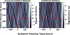 |
Fig. 6 Vyys-Kp maps for the self-consistent 100 times solar dayside model for the original temperature profile (T.1). Left panel: Vsys-Kp map in terms of the S/Np computed from the cross-correlation coefficients. Right panel: Vsys-Kp map in terms of the significance computed from the likelihood (see Sect. 5.4). Neither map shows a significant peak at the known orbital parameters of the planet (Vsys = 0kms−1, Kp = 224kms−1), indicated by the crosshairs. |
5.4 Measuring the significance of a detection
For maps of cross-correlation coefficients, the detection strength of a signal is typically measured by dividing the map by its noise, converting the coefficients into a signal-to-noise ratio (here S/Np to distinguish it from the stellar signal-to-noise ratio). The noise was taken to be the standard deviation of the map excluding the region around the expected location of the planetary signal and a S/Np of five or more is typically needed for a robust detection. The left panel in Fig. 6 shows an example Vsys-Kp map in terms of S/Np which was calculated from the cross-correlation coefficients by dividing each row by its standard deviation excluding a 60kms−1 swath around Vsys = 0kms−1 to exclude any possible planetary signal. There is no signal from the planet in this map which would appear as a peak at Vsys = 0kms−1 and Kp = 224kms−1.
For map of likelihoods, the detection strength was determined by converting the likelihood values to a significance. In this work, we used the process described in more detail in Appendix D of Pino et al. (2020), which has often been used in HRCCS exoplanet characterisation (Lafarga et al. 2023; van Sluijs et al. 2023; Dash et al. 2024; Parker et al. 2025). This method uses Wilks’ theorem Wilks (1938) which states that the test statistic (Eq. (6)) follows a χ2 distribution in the limit of large sample sizes. This distribution has degrees of freedom equal to the difference in degrees of freedom between the null hypothesis, that the orbit of the planet is described by a specific pair of (Vsys,null, Kp,null), and the alternative hypothesis, where the orbital parameters are allowed to vary. In this case this means the χ2 distribution has two degrees of freedom.
The survival function of the χ2 provides the probability that the likelihood measured for an alternative set of parameters (Vsys,alt, Kp,alt) would occur by chance if the parameters for the null model (Vsys,null, Kp,null) were the true values. If the alternative models all have small probabilities, this implies that the null model represents an increase in the likelihood above the level expected for noise. To quantify this in an intuitive way, we converted the probabilities to significances using a Gaussian distribution.
We computed the test statistics, where the null model, (Vsys,null, Kp,null), has the maximum likelihood, Lmax, in the map
![Mathematical equation: \lambda = 2 [\text{log}(L_{\text{max}}) - \text{log}(L)] .](/articles/aa/full_html/2026/01/aa57240-25/aa57240-25-eq13.png) (6)
(6)
The null model may not necessarily have the expected Vsys = 0kms−1 and Kp = 224kms−1 for LTT-9779b. If it similar, it could simply be due to fluctuations in the noise. However, if the null parameters are significantly different, then this means the planet was detected as its signal is below the noise level.
Converting this test statistic to significance as described creates a Vsys - Kp map where the highest peak has a significance of zero and all other points have positive significance. To determine if this highest peak is significantly above the noise level in the map we followed Parker et al. (2025). So that this map has a similar behaviour to that of the more traditional cross-correlation maps where the planetary signal would form a positive peak, we converted the significances in the map using the following metric:
 (7)
(7)
We considered ∆σ > 5 a robust detection. The right panel in Fig. 6 shows the same map as the left panel but now in terms of likelihoods converted to significances. This map also shows no signal from the planet. In what follows we chose to only use the likelihood maps and their significances as this measure is more robust than the cross-correlation S/Np. This is because the latter can be dependent on the region selected for calculating the standard deviation. The likelihood version is also easier to compare and combine with lower resolution methods.
5.5 Defining an equivalent uniform volume-mixing ratio
The S/Np or significance at which a spectrum is recovered using high-resolution cross-correlation spectroscopy is strongly dependent on the number of spectral lines and their depth. The exact number and depth of lines is a complex function of the atmospheric parameters however, it is useful to understand when these numbers might be similar for different models. To achieve this, we defined the equivalent uniform volume-mixing ratio, EUVMR, as the VMR that for a uniform profile would result in the same column mass of a given species above the clouds as a more complex profile.
This parameter is a good metric for determining when two models have a similar number and depth of spectral lines from a given species because the depth of the spectral lines is related to their optical depth, τ, which is give by
 (8)
(8)
where X is the mass fraction of the species, κ its opacity, g the gravitational acceleration and P the atmospheric pressure. Assuming the opacity is constant with pressure and that g is also approximately constant, which is valid for the upper parts of the atmosphere. Then the optical depth and therefore depth of the spectral lines is proportional to the integrated mass fraction which is proportional to the column mass of the species.
Therefore, the line depths approximately proportional to the column mass of the species. This integral needs to be limited to the atmosphere above the clouds if the clouds are optically thick as the atmosphere beneath them does not contribute to the spectrum.
Phase range split.
5.6 Model injection to test the data sensitivity
The sensitivity of these data to different types of planetary spectra can be determined by testing whether or not an injected model is recovered using this analysis. To be realistic, the injected spectrum must be processed in the same way as the real spectrum. Therefore it must be injected into the data as early as possible in the analysis. As discussed in Sect. 4.1, the first few steps in the data reduction involved continuum normalisation, subtracting the median spectrum and removing outliers. The first two of these may affect the embedded planetary spectrum, but the outlier removal itself is unlikely to have a strong impact. Unfortunately, the blob detection algorithm used for the outlier removal is very computationally expensive. Thus we injected the model after this step. However, to account for the effect continuum normalisation and subtracting the median spectrum might have on the injected spectrum, the median spectrum was added back into the data and continuum restored before the model was injected. Therefore, the injected spectrum was treated in largely the same way as any real spectrum in the data.
The injection was achieved by first measuring the continuum level of each order of each observation. This was done by fitting a linear trend to the spectrum excluding any deep spectral lines which were defined as those points lying more than three sigma away from the linear trend. This trend was assumed to represent the flux of the star in these data, and thus, the planetary spectrum would be equivalent to this trend multiplied by a model of the planet-to-star contrast ratio. This model of the contrast ratio spectrum was first Doppler-shifted to the planetary velocity, but with the orbital velocity taking the opposite sign to ensure it is not injected on top of any real planetary spectra in the data. It was then multiplied by the linear trend, creating a model of the planetary flux in terms of data units, and added into the data. The data reduction and analysis then proceed as before.
6 Results
6.1 A non-detection of the reflected light of LTT-9779 b
As discussed in Sect. 5.2.1, the self-consistent spectral models were generated for three different segments of the planetary dayside: eastern dayside, dayside, and western dayside. These are observable at different points in the planets orbit, and we therefore split our reduced data into three sets based on the orbital phase of LTT-9779 b (see Table 5). On each set of observations, we performed the likelihood analysis using only the models for the corresponding dayside segment. We observed no robust detection, with ∆σ > 5 or S/Np > 5, of the reflected-light spectrum of LTT-9779 b for any of the self-consistent spectral models. Fig. 6 shows the Vsys-Kp maps for 100 times solar dayside model for the original temperature profile both in terms of cross-correlation S/Np and likelihood significance, ∆σ.
Similar to the self-consistent spectral models, the singlespecies models discussed in Sect. 5.2.2 used two different cloud models (C.1 and C.2 in Table 4) that match the albedo measured by JWST NIRISS/SOSS for the eastern (pre-eclipse) and western (post-eclipse) hemispheres of LTT-9779 b. We therefore split the observations into pre- and post-eclipse and run the analysis only for the models corresponding to that part of the orbit. While these models contain only one species, and so would not perfectly match the real spectrum of LTT-9779 b, a detection with these models can be used as a start point for an atmospheric retrieval which would reveal the planetary spectrum in more detail. Unfortunately, we observed no robust detection (∆σ > 5 or S/Np > 5) of the reflected-light spectrum of LTT-9779 b for any of the single-species spectral models.
A lack of a robust detection does not imply that the planet is not reflective, simply that its high-resolution reflection spectrum is not detectable with the current data as the HRCCS technique relies on the presence of a large number of deep spectral lines.
6.2 A word of caution on false positives
The Vsys-Kp map for the post-eclipse data with the single-species Fe model that has a VMR of Fe equal to 10−2 and a cloud top pressure of 10−1.5 bar is shown in Fig. 7. In this map, there is a significant peak at Vsys = 38kms−1 and Kp = 286 km s−1 when all the observations were combined. This is offset from the expected orbit, which is represented by Vsys = 0 km s−1 and Kp = 224kms−1, by an amount that is not easily explained by one or a combination of atmospheric dynamics (see Fig. 9 in Snellen 2025, and references therein), errors in the ephemeris (see Sect. 3 and Meziani et al. 2025) or limb asymmetry Hoeijmakers et al. (2024).
Normally, a detection threshold of ∆σ = 5 is used for determining when a signal is significantly detected and while the signal here has ∆σ ≈ 6.7, it is a false-positive. This is because, due to the modelled atmospheric conditions in the lower atmosphere, the iron lines present in this and similar model spectra have broad profiles. In most HRCCS analyses, the width of the spectral lines is approximately the same as the resolution element of the observations. When the spectral lines are significantly broader than the resolution element, this Doppler-shift sampling creates correlations in the noise present in the Vsys-Kp map. This lowers the standard deviation of the noise, which results in more significant false-positive peaks. A visual inspection revealed that most of the spectral lines have been broadened meaning we could not simply exclude the broad lines from the template. Parker et al. (2024) discussed how downsampling the velocity resolution in the analysis to the width of the broadened model template can mitigate correlated noise. For this model, the full-width half-maximum of the autocorrelation function is approximately 26 km s−1. We therefore downsampled the velocity resolution by using only every 32nd Doppler shift from the original analysis. When we created the Vsys-Kp map with this reduced sampling, the peak shown in Fig. 7 reduces in significance to ∆σ < 5.
6.3 Constraining the atmospheric parameters of LTT-9779b via injection tests
To learn more from the non-detection, we can perform two types of injection tests to constrain the properties of LTT-9779 b. First, we could assume the spectrum of the planet contains specific set of spectral lines of known depth and vary the broadband albedo of the model such as in Spring et al. (2022). This would constrain the broadband albedo however, it is difficult to implement for LTT-9779 b since we do not have enough information on the deep spectral lines present. This is because the stellar lines cannot be used in this analysis due to strong rotational broadening and prior constraints do not allow us to confidently predict which atmospheric spectral lines will be present. Therefore, we elected not to perform this test, as the results will be highly dependent on which model we chose to use for the spectrum of LTT-9779 b and the albedo had already been measured at low spectral resolution.
The second type of injection test assumes instead that the broadband albedo is known and that the type and depth of the spectral lines are varied. This type of test can put constraints on the abundances of the species in the atmosphere of LTT-9779 b and on altitude of the cloud deck. We elected to perform this type of test. Models were injected into the data prior to the main data reduction as described in Sect. 5.6 and the analysis proceeded as described in Sects. 4 and 5. Fig. 8 shows an example of the Vsys-Kp map from an injection-recovery test in which the injected model was recovered at high significance. This means that this model cannot represent the planetary spectrum as no detection was made with the original data.
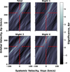 |
Fig. 7 Top left panel: Vsys-Kp map for for the single-species Fe model with a VMR of 0.01 and a cloud top pressure of 10−1∙5 bar for all post-eclipse data containing a significant false-positive signal. The red crosshairs indicate the expected location of the planetary signal. The remaining three panels show the corresponding maps for each of the observing nights individually. There is no map for night 3 as no posteclipse data were taken. |
6.3.1 Sensitivity to the self-consistent spectral models
Section 5.2.1 introduces the self-consistent spectral models which used atmospheric parameters measured by JWST NIRISS/SOSS for three segments of the planetary dayside: eastern dayside, dayside, and western dayside. These different segments are observable at the orbital phases given in Table 5.
For each type of temperature profile (T.1 and T.2 in Table 4) and chemistry (Ch. 1, Ch. 2 and Ch. 3 in Table 4) we injected the three different segment models into the observations of the corresponding orbital phases. The data were reduced as described in Sect. 4 and the reduced observations split up into three sets based on which of the three segment models were injected. The likelihood analysis was performed on each of the three sets as described in Sect. 5 using the injected spectrum as the model in the likelihood analysis (g in Eq. (1)).
In Figs. 9 and 10, the significance at which a given model was recovered is indicated by the colour of the associated square where black indicates that the model was not recovered. We consider ∆σ > 5 as the threshold for a confident detection. For the models with the original temperature profile (T.1 in Table 4), only the high-metallicity dayside and western dayside models containing all species were detectable. With the modified temperature profile (T.2 in Table 4), only the intermediate metallicity dayside models were detectable. These correspond to models with higher albedo and a large number of deep spectral lines. An interesting point to note is that the recovered significance matches with predictions made with synthetic observations used to design these observations (see Sect. 2).
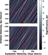 |
Fig. 8 Example of an injection-recovery test. Top panel: Vsys-Kp map when the true observations are compared to the self-consistent 100 times solar western dayside model with the original temperature profile. Bottom panel: Vsys-Kp map when the same model was injected into the data at a negative orbital velocity (reversed y -axis). The expected location of the signal is indicated by the crosshairs in both panels. |
6.3.2 Sensitivity to the single-species spectral models
The single-species models are introduced in Sect. 5.2.2 with each model containing one species (TiO, VO, Fe, MgH, FeH, H2O or AlH). The models for each species were split into two sets, one that matches the albedo measured by Coulombe (2025) in pre-eclipse JWST NIRISS/SOSS observations (C.1 in Table 4) and another matching the post-eclipse (C.2 in Table 4). For each species and each set, the models form a grid in which the VMR and the height of the cloud deck are varied.
Since the two sets of models, C.1 and C.2 in Table 4, were associated with different orbital phases, we once again injected these models into the observations of the corresponding orbital phase. The data were reduced as described in Sect. 4 and the reduced observations split up into pre- and post-eclipse. The likelihood analysis in Sect. 5 was performed on these two sets separately using the injected spectrum as the model in the likelihood analysis (g in Eq. (1)). We note that as discussed in Sect. 6.2, some of the iron models have spectral lines much broader than the resolution element. For these we downsampled the velocity resolution assuming the average broadening; 20kms−1.
Fig. 11 show the significance, ∆σ, with which each injected model was recovered for the post-eclipse data and Fig. 12 shows the same for the pre-eclipse. Again, a black square in the plots indicates the model was not recovered. In post-eclipse we were able to recover some of the TiO, VO, Fe, MgH, FeH and H2O models whereas in pre-eclipse we were only able to recover some VO, MgH and FeH models. This is because even though we had more pre-eclipse data, the eastern hemisphere of the planet has a lower albedo (Coulombe et al. 2025) making its spectrum fainter and harder to characterise. The models with lower altitude cloud decks and higher abundances typically have deeper lines and were therefore detected at higher significance. This was not true of all models as in some cases the spectral lines start strongly saturating. When this happened, the saturation lowers the continuum of the spectrum which decreases the difference in contrast between the continuum and the minimum of the spectral line. This further lowered the signal-to-noise ratio of the spectral lines embedded in the data and therefore the S/Np at which the planet’s spectrum could be recovered. Additionally, the saturating spectral lines tended to become much broader which caused the continuum normalisation to absorb some of the line. This lowered the contrast between the line and continuum and thus lowered the recovered S/Np of the spectrum. The combination of these effects made some of the models with the highest abundances and deepest cloud decks undetectable with these data.
Section 5.5 introduces a method of identifying models that would be recovered at similar significance by comparing their EUVMRs. For the single-species models, the EUVMR is equivalent to the VMR of the species. Therefore these injection tests represent the range of EUVMRs that were detectable for each species, for a given cloud deck height in these data. In Table 6, we summarise the EUVMRs of each species that can be ruled out as a result of this non-detection assuming the cloud deck was at the altitude predicted by the JWST NIRISS/SOSS data. With the exception of TiO in the post-eclipse data (see Sect. 7.1 for further discussion) these restrictions are consistent with equilibrium chemistry. Due to the observed wavelength range, we were not sensitive to CH4, CO and CO2 hence we were unable to restrict the EUVMRs of these species.
Comparing these restrictions with the literature, we see that the pre-eclipse restriction on FeH is consistent with the work of Edwards et al. (2023) and Zhou et al. (2025) which constrained the VMRFeH ∼ 10−8 in the terminator atmosphere. Additionally, the restrictions on TiO and VO are more consistent with the constraints imposed by Edwards et al. (2023) of VMRTiO < 10−8 and VMRvo < 10−9 for the terminator atmosphere over those imposed by Reyes et al. (2025) which constrained the metallicity to greater than 180 times solar corresponding to VMRTiO ≳ 10−7 and VMRvo ≳ 10−8. The discrepancy between the constraints imposed by these two works is due to the clouds of LTT-9779 b which flatten the transit spectrum. Reyes et al. (2025) do not include clouds in their model so the flattening of the spectrum is instead caused by increasing the TiO and VO abundances. The clouds in Edwards et al. (2023) are lower in the atmosphere than assumed in Table 6, hence their lower constraint on the VMRs of TiO and VO.
The restrictions on the EUVMR imposed by these injections come with a caveat: since the model injected and the model used in the likelihood analysis are the same, they represent a ‘best case scenario’. This is because the real spectrum will be slightly different to the model and also contain the spectral lines of other species which may interfere with the lines of the chosen species. A more comprehensive test would have been to inject a full model containing all species, which would then be recovered with the single-species models. However, since we were not assuming equilibrium chemistry, this leads to an infeasibly large number of models containing all species at varying abundances and thus it was not possible to perform these injection tests.
 |
Fig. 9 Results of the injection-recovery test on the self-consistent models with the original temperature profile (T.1 in Table 4). The black square indicates that the highest likelihood peak exceeded 50kms−1 in Vsys or Kp from the expected location of the injected orbit. The coloured squares indicate the significance (∆σ) at which the injected spectrum was recovered. The grey squares indicate the models that were recovered at ∆σ < 5. |
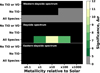 |
Fig. 10 Same as Fig. 9, but for models created with the modified isothermal temperature profile (T.2 in Table 4). |
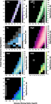 |
Fig. 11 Significance, ∆σ, at which the model is recovered in the injection-recovery test on the single-species models for the post-eclipse observations. The black square indicates that the model was not recovered in the injection-recovery tests. The coloured squares indicate the significance at which the injected spectrum was recovered. The grey squares indicate the models that were recovered at ∆σ < 5. |
6.3.3 Determining the sensitivity to new spectral models
As discussed in Sect. 5.5, models with similar numbers and depths of spectral lines are expected to be recovered at similar significances. The number and depth of spectral lines is similar for models with the same EUVMRs. Further, the single-species injection tests revealed the range of EUVMRs for each species that would be detectable with these data as a function of the altitude of the top of the cloud deck. Therefore, by computing the EUVMR of a more complex model, and comparing it to the results of the single-species injection test, we can determine if that model should have been detected with these data without the need for further injection tests. Additionally, as the singlespecies models did not result in a detection, these more complex models can be ruled out.
We demonstrate this method for ruling out new models in Figs. 13 and 14. In these plots we once again show the results of the single-species injection test but with different colour coding. Here, all the models recovered with ∆σ > 5 are highlighted in light brown. Additionally, highlighted in dark brown are models for which the saturation of spectral lines has reduced the average contrast ratio of the model to at least three sigma below the contrast of LTT-9779 b measured by JWST NIRISS/SOSS. Together, these two regions highlight the models ruled out but these and previous data. Next, we computed the EUVMRs as a function of the height of the cloud deck for the full self-consistent chemical equilibrium model (Ch.1 in Table 4) for the eastern and western dayside. These profiles cover a range of metallicities from 0.1 times solar to 1000 times solar and two versions of the temperature profile (T.1 and T.2 in Table 4).
The EUVMRs as a function of the height of the cloud deck for the western dayside (approximately post-eclipse) are plotted in Fig. 13 and those for the eastern dayside (approximately preeclipse) in Fig. 14. This shows, if we were to vary the altitude of the cloud in the self-consistent models, whether the resulting spectrum would have been detectable in these data.
The predictions made using the EUVMRs match closely to the results of the self-consistent model injections tests shown in Figs. 9 and 10. For example, the EUvmrs of each species in the pre-eclipse data shown in Fig. 14 do not fall within the detectable region at a cloud top pressure of 10−1.5 bar. This is consistent with none of the eastern dayside self-consistent models being recovered in the injection tests. Likewise for the post-eclipse data, the EUVMRs of TiO predicts that the 1 times to 1000 times solar models for the original temperature profile (T.1 in Table 4) and the 1 times and 10 times solar models for the modified temperature profile (T.2 in Table 4) will be detectable for a cloud top pressure of 10−4 bar. This matches with the injection tests for the dayside models, which have a similar albedo to the posteclipse models. The exception is the dayside 100 times solar, modified temperature-profile model which was detected in the injection test but is not predicted to be. Since the self-consistent models contain the multiple species, they will be recovered at higher significance than predicted using the EUVMR of a single species and this model has an EUVMR for TiO close to the detection limit. The predictions do not match as well with the injection tests for the western dayside models where the injection tests did not recover, as predicted, the 1 times solar, original temperatureprofile model or any of the modified temperature-profile models. This discrepancy was likely caused by the difference in the phase range of the injection tests. The injection tests used to predict the detectability in Figs. 13 and 14 were for the entire pre- and post-eclipse data whereas the self-consistent model injections split the data into eastern dayside, dayside and western dayside. The detection strengths of the self-consistent models do correlate with the EUVMR since models with higher EUVMR are detected with greater significance, ∆σ. This highlights the usefulness of this method of comparison.
Restrictions placed on the EUVMR of different species by these data.
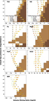 |
Fig. 13 Restrictions placed on the vMR as a function of cloud deck altitude for the post-eclipse observations. The injection-recovery tests presented here rule out the models in light brown. Additionally, we highlight the models in dark brown which, due to the saturation of a large number of the spectral lines, have an average contrast ratio more than three sigma below the contrast of LTT-9779 b at these wavelengths measured by JWST NIRISS/SOSS data. To compare these restrictions to more complex models, we also plot the EUVMRS for metallicities ranging from 0.1 times solar to 1000 times solar as a function of the altitude of the cloud deck for the original (T.1, circles) and modified (T.2, crosses) temperature profiles for the western dayside. |
7 Discussion
7.1 Non-detection of TiO
Previous observations have suggested that TiO might be depleted in the atmosphere of LTT-9779 b. As discussed in Sect. 6.1, we did not detect the reflected-light spectrum of LTT-9779 b in these data. However, as shown in Sect. 6.3.1 we should have been sensitive to spectral models based on data from previous observations, assuming high metallicity with TiO at its equilibrium abundance, in the post-eclipse data. Therefore, this non-detection might indicate a depletion of TiO in the westernhemisphere of LTT-9779 b. To determine if our non-detection is a result of TiO depletion, we considered the following alternative possibilities: (1) TiO is present at its equilibrium abundance but the spectral lines are reduced in size by a high-altitude cloud deck, (2) the temperature profile is different to what was previously measured and TiO is not expected in significant quantities, and (3) the combination of these two alternatives. To explore these alternatives, we compared the EUVMRs of the self-consistent western dayside models with the results of the single-species TiO injection test shown in the top left panel of Fig. 13.
To explore whether TiO could still be present at its equilibrium abundance but hidden by a high-altitude cloud deck, we studied the TiO EUVMRs for the western dayside with the original temperature profile (T.1 in Table 4). In the top left panel of Fig. 13 the TiO EUVMRs for the original temperature profile are shown as circles. The high metallicity versions of these EUVMRs fall within either the light or dark brown ruled out regions. This implies that if the atmosphere of LTT-9779 b is high metallic-ity and the western dayside follows the original T.1 temperature profile, then the cloud deck would need to be above 10−5 bar for these data to result in a non-detection of TiO assuming it is present at its equilibrium abundance. To understand if changing the temperature profile changes the expected TiO abundance significantly enough to change this result, we also studied the TiO EUVMRs for the modified temperature profile (T.2 in Table 4; shown as crosses in Fig. 13). The modified temperature profile lowers the EUVMRs in the highest and lowest metallicity models. This results in cloud decks above 10−2 bar becoming effective at shielding the presence of TiO at its equilibrium abundance for these metallicities. However, for intermediate (10 times solar) metallicities, the cloud deck would once again need to be over 10−5 bar to have the same effect.
Ultimately, with the uncertainty in the upper temperature profile and the metallicity, it is not possible to say for certain if our non-detection was a result of TiO depletion in the western atmosphere of LTT-9779 b. However, since the non-detection of TiO would require extreme cloud altitudes for more than half of our high metallicity models, we argue that depletion is currently the more likely reason for our non-detection. This conclusion comes with a caveat: we assumed our TiO line list was accurate enough that the model lines would correlate well with any real TiO lines present in the planetary spectrum. We used the same line list as in Prinoth et al. (2022), Prinoth et al. (2023), and Prinoth et al. (2025). In the former two works, this line list was able to detect the presence of TiO on WASP-189 b and in the latter a non-detection of TiO on WASP-121b was presented. For WASP-189b, the signal of TiO recovered was five to six times weaker than that of an injected isothermal model which was attributed to inaccuracies in the line lists. Similarly, for WASP-121 b a detection of Ti I was in tension with the nondetection of TiO which might indicate that inaccuracies in the line list caused the non-detection as opposed to a lack of TiO. These works would imply that our non-detection of TiO was largely due to inaccuracies in the line lists. However, subsequent low-resolution observations WASP-121 b have indicated a strong depletion of TiO (Pelletier et al. 2025; Saha & Jenkins 2025). We argue that it is ultimately difficult to quantify how well the line list performs without knowing the true abundance of TiO on the exoplanets that are studied. This is difficult to determine, as we highlighted above.
7.2 Constraints of the cloud properties
LTT-9779 b is a cloudy world. Studies of the terminator atmosphere have favoured a low cloud deck at approximately 1 bar (Edwards et al. 2023; Zhou et al. 2025). Since the dayside of the planet is hotter than the terminator, we would expect to find a higher cloud deck on the dayside. However, the altitude of the dayside cloud deck is not well constrained (Coulombe et al. 2025). As discussed in Sect. 1, understanding this world and its place in the desert requires detailed information on its atmosphere. Current studies are hindered by the degeneracy between the altitude of the cloud deck, and the metallicity of this atmosphere. These data allows us to improve restrictions on the altitude of the cloud deck, thus partly breaking this degeneracy.
The restrictions we place on the altitude of the cloud deck are informed by the non-detection of MgH in both the pre- and posteclipse data (see Sect. 6.1). The single-species injection test for MgH, shown in Figs. 11 and 12, revealed the range of EUVMRs for MgH that could be ruled out as a result of this non-detection. We then compared this with the EUVMRs for MgH predicted from equilibrium chemistry models to determine at what altitudes the cloud deck obscures the MgH spectral features enough to prevent detection. Figures 13 and 14 show EUVMRs for MgH predicted from equilibrium chemistry for two different temperature profiles (T.1 and T.2 in Table 4) along with the parameter space ruled out by this non-detection and previous data. Comparing the EUVMRs for the two temperature profiles, it is clear that the MgH abundance is not very sensitive to temperature. This makes it ideal for investigating the altitude of the cloud deck. Assuming, as suggested by previous observations, that this planet has a high metallicity we compared the EUVMRs for the 10 times, 100 times and 1000 times solar models. Fig. 13 indicates that our post-eclipse data should have been sensitive to MgH at the EUVMRs predicted for the high metallicity models when the top of the cloud deck is at pressures greater than 10−2 bar. Thus, the cloud deck of LTT-9779 b must be at pressures lower than 10−2 bar in the western hemisphere. Likewise, Fig. 12 indicates that our pre-eclipse data should have been sensitive to MgH if the cloud deck was at pressures greater than 10−0.5 bar, hence the top of the cloud deck in the eastern-hemisphere must be at lower pressures.
7.3 A pathway to the detection of reflected light at high spectral resolution
These data were taken with ESPRESSO in 4-UT mode with just under 9 hours spent on pre-eclipse and 5 hours and 40 minutes on post-eclipse. These observations have an average S/N ≈ 160 at λ = 530nm. We note that LTT-9779 (V = 9.79 mag) is on the fainter end of stars that can be characterised at high resolution hence why we used the greater collecting area of the ESPRESSO 4-UT mode for these observations. Unfortunately, despite the high albedo of LTT-9779 b, we did not detect its highresolution reflection spectrum which implies this planet lacks the large number of deep spectral lines required for this technique to work.
This highlights that the broadband albedo is not necessarily a good indication of detectability with the HRCCS technique as this does not necessarily imply the spectrum has enough deep lines to be detected. Thus we suggest the best targets to characterise with this technique using current instrumentation have the following properties; (1) A medium to high albedo as this increases the signal-to-noise of the planets spectrum, (2) A low altitude cloud deck, and (3) High metallicity. In addition to these three points it would also be more favourable to have (1) A brighter host star than LTT-9779, (2) A longer orbital period to reduce the rotational broadening of the reflected stellar spectrum so that the stellar lines could be used in the cross-correlation templates, and (3) A planet in the transiting configuration because these tend to have much more precise ephemerides.
It is not long before the ELT comes online. Its armazones high dispersion echelle spectrograph (ANDES) instrument will be able to take observations similar to ESPRESSO, but at R = 100,000, over a wider wavelength range of 0.4–1.8 μm, and on a larger telescope (Palle et al. 2025; Marconi et al. 2024). The ANDES ETC7 indicates that ANDES will reach an S /N ≈ 740 at λ = 530 nm in 200 s assuming a G8V star with a V-band magnitude of 9.79 at an airmass of 1.3. When compared to these ESPRESSO observations, which reach S/N ≈ 160 at λ = 530 nm in 200 s, this is an improvement by 4.6 times in the S/N as a function of time, which is a result of the larger primary mirror and better instrumental throughput. This vast improvement in the S/N and extended wavelength range will open up the characterisation of LTT-9779 b as other atmospheric species are predicted to become characterisable with the improvement in S/N using a similar amount of observing time to that already obtained. Additionally, this will open up the characterisation of even more worlds in reflected light from giant planets to potentially some rocky worlds (see e.g. Palle et al. 2025). While characterising rocky worlds will be challenging, simulations of similar observations using the high angular resolution monolithic optical and near-infrared integral field spectrograph (HARMONI), which will also be on the ELT but has a lower spectral resolution, have shown that such worlds can be characterised (Vaughan et al. 2024). In all cases, the detectability of the reflected-light spectrum of a planet at high spectral resolution is dependent on it possessing a large number of deep spectral lines.
8 Conclusions
We used four half-nights of ESPRESSO 4-UT mode observations to characterise the reflected-light spectrum of LTT-9779 b at high spectral resolution. We list our conclusions from these observations below.
In these data, we were unable to robustly detect the reflected-light spectrum of LTT-9779 b despite its known high albedo. We expected to detect TiO in the dayside and western dayside spectrum for a range of different metallicities and assumptions on the temperature profile. Therefore, this nondetection might imply a depletion of TiO compared with equilibrium chemistry. This depletion might be caused by the cold trapping of TiO and is consistent with the lack of a thermal inversion (Dragomir et al. 2020). We also showed, however, that the abundance of TiO in chemical equilibrium, and therefore, its detectability, is sensitive to the temperature in the upper atmosphere at P < 10 μbar. Therefore, it is currently not possible to determine whether the non-detection of TiO is due to depletion because of the uncertainty in its equilibrium abundance.
A non-detection of MgH post-eclipse indicates that the cloud pressure on the western dayside is lower than 10−2 bar, and the non-detection of MgH pre-eclipse indicates that the eastern dayside cloud pressure is lower than 10−0.5 bar. This is consistent with predictions of MgSiO3 and Mg2SiO4 clouds based on the mean JWST NIRISS/SOSS temperature profile.
The atmospheric characterisation we presented also highlighted a false-positive detection. We determined that this was due to an oversampling in the Vsys-Kp map because in this case, the majority of the Fe lines are broader than the instrumental resolution. This created correlated noise. We therefore recommend caution when interpreting HRCCS detections made with models containing broad spectral lines.
In addition to the atmospheric characterisation, we also reviewed the orbit of this planet. By combining these data with previous observations, we computed an updated ephemeris. Our orbit fits favour a circular orbit, but there is some indication of a non-zero eccentricity. This requires more data for confirmation, but if confirmed, it might be an indication of high-eccentricity migration.
Finally, we discussed the future of high spectral resolution characterisations of exoplanets in reflected light with the VLT and the upcoming ELT. The unrivalled collecting area of the ELT will further the characterisation of LTT-9779 b and open the door to many other worlds. As we have highlighted here, even very reflective exoplanets might not be detectable at high spectral resolution if they lack deep spectral lines. We therefore advise caution when selecting targets for observations.
Acknowledgements
This work is based on observations collected at the European Organisation for Astronomical Research in the Southern Hemisphere under ESO programmes 0112.C-0367, 2103.C-5063, 0108.C-0161, 0102.C-0525, and 0102.C-0451. S.R.V., J.L.B. and L.T.P. acknowledge funding from the European Research Council (ERC) under the European Union’s Horizon 2020 research and innovation program under grant agreement No. 805445. J.S.J gratefully acknowledges support by FONDECYT grant 1240738 and from the ANID BASAL projects ACE210002 and FB210003. H.Y. acknowledge funding from the European Research Council under the European Union’s Horizon 2020 research and innovation programme (grant agreement No 865624, GPRV). J.V.S. acknowledges support from the Poincaré fellowship of the Observatoire de la Côte d’Azur. V.P. acknowledges funding by the French National Research Agency (ANR) project EXOWINDS (ANR-23-CE31-0001-01). N.E.B acknowledges support from NASA’S Interdisciplinary Consortia for Astrobiology Research (NNH19ZDA001N-ICAR) under award number 19-ICAR19 2-0041. The first author would also like to thank Paul Mollière for their discussion on atmospheric column mass and Lorena Acuna for their discussion on tidal heating.
References
- Ackerman, A. S., & Marley, M. S. 2001, ApJ, 556, 872 [Google Scholar]
- Allard, F., Allard, N. F., Homeier, D., et al. 2007a, A&A, 474, L21 [NASA ADS] [CrossRef] [EDP Sciences] [Google Scholar]
- Allard, N. F., Kielkopf, J. F., & Allard, F. 2007b, Eur. Phys. J. D, 44, 507 [NASA ADS] [CrossRef] [Google Scholar]
- Allard, N. F., Spiegelman, F., & Kielkopf, J. F. 2016, A&A, 589, A21 [NASA ADS] [CrossRef] [EDP Sciences] [Google Scholar]
- Allard, N. F., Spiegelman, F., Leininger, T., & Molliere, P. 2019, A&A, 628, A120 [NASA ADS] [CrossRef] [EDP Sciences] [Google Scholar]
- Ashtari, R., Collins, S., Splinter, J., et al. 2025, AJ, submitted [arXiv:2510.04863] [Google Scholar]
- Azzam, A. A. A., Tennyson, J., Yurchenko, S. N., & Naumenko, O. V. 2016, MNRAS, 460, 4063 [NASA ADS] [CrossRef] [Google Scholar]
- Barber, R. J., Strange, J. K., Hill, C., et al. 2014, MNRAS, 437, 1828 [CrossRef] [Google Scholar]
- Bard, A., & Kock, M. 1994, A&A, 282, 1014 [NASA ADS] [Google Scholar]
- Bard, A., Kock, A., & Kock, M. 1991, A&A, 248, 315 [NASA ADS] [Google Scholar]
- Batalha, N. E., Marley, M. S., Lewis, N. K., & Fortney, J. J. 2019, ApJ, 878, 70 [NASA ADS] [CrossRef] [Google Scholar]
- Batalha, N. E., Rooney, C. M., Visscher, C., et al. 2025, AAS Journal, submitted [arXiv:2508.15102] [Google Scholar]
- Birkby, J. L. 2018, Spectroscopic Direct Detection of Exoplanets (Springer International Publishing), 1485 [Google Scholar]
- Borsa, F., Allart, R., Casasayas-Barris, N., et al. 2021, A&A, 645, A24 [EDP Sciences] [Google Scholar]
- Brogi, M., & Line, M. R. 2019, AJ, 157, 114 [Google Scholar]
- Burrows, A., Ram, R. S., Bernath, P., Sharp, C. M., & Milsom, J. A. 2002, ApJ, 577, 986 [NASA ADS] [CrossRef] [Google Scholar]
- Coppola, C. M., Lodi, L., & Tennyson, J. 2011, MNRAS, 415, 487 [NASA ADS] [CrossRef] [Google Scholar]
- Coulombe, L.-P. 2025, Data for ‘Highly reflective white clouds on the western dayside of an exo Neptune’. [Google Scholar]
- Coulombe, L.-P., Radica, M., Benneke, B., et al. 2025, Nat. Astron., 9, 512 [Google Scholar]
- Crossfield, I. J. M., Dragomir, D., Cowan, N. B., et al. 2020, ApJ, 903, L7 [NASA ADS] [CrossRef] [Google Scholar]
- Dash, S., Brogi, M., Gandhi, S., et al. 2024, MNRAS, 530, 3100 [Google Scholar]
- Dragomir, D., Crossfield, I. J. M., Benneke, B., et al. 2020, ApJ, 903, L6 [NASA ADS] [CrossRef] [Google Scholar]
- Dulick, M., Bauschlicher, C. W. J., Burrows, A., et al. 2003, ApJ, 594, 651 [NASA ADS] [CrossRef] [Google Scholar]
- Edwards, B., Changeat, Q., Tsiaras, A., et al. 2023, AJ, 166, 158 [NASA ADS] [CrossRef] [Google Scholar]
- Fernandez, J. F., Wheatley, P. J., King, G. W., & Jenkins, J. S. 2023, MNRAS, 527, 911 [CrossRef] [Google Scholar]
- Foreman-Mackey, D., Luger, R., Agol, E., et al. 2021, J. Open Source Softw., 6, 3285 [NASA ADS] [CrossRef] [Google Scholar]
- Fortney, J. J., Mordasini, C., Nettelmann, N., et al. 2013, ApJ, 775, 80 [Google Scholar]
- Fortney, J. J., Visscher, C., Marley, M. S., et al. 2020, AJ, 160, 288 [NASA ADS] [CrossRef] [Google Scholar]
- Fu, G., Mukherjee, S., Stevenson, K. B., et al. 2025, ApJ, 989, L17 [Google Scholar]
- Fuhr, J. R., Martin, G. A., & Wiese, W. L. 1988, J. Phys. Chem. Ref. Data, 17, 4 [Google Scholar]
- Gandhi, S., Brogi, M., & Webb, R. K. 2020, MNRAS, 498, 194 [Google Scholar]
- Gharib-Nezhad, E., Shayesteh, A., & Bernath, P. F. 2013, MNRAS, 432, 2043 [NASA ADS] [CrossRef] [Google Scholar]
- Gharib-Nezhad, E., Iyer, A. R., Line, M. R., et al. 2021, ApJS, 254, 34 [NASA ADS] [CrossRef] [Google Scholar]
- Ginzburg, S., Schlichting, H. E., & Sari, R. 2018, MNRAS, 476, 759 [Google Scholar]
- Gordon, I. E., Rothman, L. S., Hargreaves, R. J., et al. 2022, J. Quant. Spec. Radiat. Transf., 277, 107949 [NASA ADS] [CrossRef] [Google Scholar]
- Gordon, I. E., Rothman, L. S., Tan, Y., Kochanov, R. V., & Hill, C. 2017, in 72nd International Symposium on Molecular Spectroscopy, TJ08 [Google Scholar]
- Gupta, A., & Schlichting, H. E. 2019, MNRAS, 487, 24 [Google Scholar]
- Gupta, A., & Schlichting, H. E. 2020, MNRAS, 493, 792 [Google Scholar]
- Gupta, A., & Schlichting, H. E. 2021, MNRAS, 504, 4634 [NASA ADS] [CrossRef] [Google Scholar]
- Gupta, A., Nicholson, L., & Schlichting, H. E. 2022, MNRAS, 516, 4585 [NASA ADS] [CrossRef] [Google Scholar]
- Hargreaves, R. J., Hinkle, K. H., Bauschlicher, Charles W. J., et al. 2010, AJ, 140, 919 [NASA ADS] [CrossRef] [Google Scholar]
- Harris, G. J., Tennyson, J., Kaminsky, B. M., Pavlenko, Y. V., & Jones, H. R. A. 2006, MNRAS, 367, 400 [Google Scholar]
- Hoeijmakers, H. J., Schwarz, H., Snellen, I. A. G., et al. 2018a, A&A, 617, A144 [NASA ADS] [CrossRef] [EDP Sciences] [Google Scholar]
- Hoeijmakers, H. J., Snellen, I. A. G., & van Terwisga, S. E. 2018b, A&A, 610, A47 [NASA ADS] [CrossRef] [EDP Sciences] [Google Scholar]
- Hoeijmakers, H. J., Kitzmann, D., Morris, B. M., et al. 2024, A&A, 685, A139 [NASA ADS] [CrossRef] [EDP Sciences] [Google Scholar]
- Hoyer, S., Jenkins, J. S., Parmentier, V., et al. 2023, A&A, 675, A81 [NASA ADS] [CrossRef] [EDP Sciences] [Google Scholar]
- Huang, X., Gamache, R. R., Freedman, R. S., Schwenke, D. W., & Lee, T. J. 2014, J. Quant. Spectr. Rad. Transf., 147, 134 [Google Scholar]
- Høg, E., Fabricius, C., Makarov, V. V., et al. 2000, A&A, 355, L27 [Google Scholar]
- Jackson, B., Arras, P., Penev, K., Peacock, S., & Marchant, P. 2017, ApJ, 835, 145 [NASA ADS] [CrossRef] [Google Scholar]
- Jenkins, J. S., Díaz, M. R., Kurtovic, N. T., et al. 2020, Nat. Astron., 4, 1148 [Google Scholar]
- Kausch, W., Noll, S., Smette, A., et al. 2015, A&A, 576, A78 [NASA ADS] [CrossRef] [EDP Sciences] [Google Scholar]
- Kokori, A., Tsiaras, A., Edwards, B., et al. 2023, ApJS, 265, 4 [NASA ADS] [CrossRef] [Google Scholar]
- Kong, H., Akakin, H. C., & Sarma, S. E. 2013, IEEE Trans. Cybernetics, 43, 1719 [Google Scholar]
- Koskinen, T. T., Lavvas, P., Huang, C., et al. 2022, ApJ, 929, 52 [NASA ADS] [CrossRef] [Google Scholar]
- Lafarga, M., Brogi, M., Gandhi, S., et al. 2023, MNRAS, 521, 1233 [Google Scholar]
- Leconte, J., Chabrier, G., Baraffe, I., & Levrard, B. 2010, A&A, 516, A64 [NASA ADS] [CrossRef] [EDP Sciences] [Google Scholar]
- Lee, E. J., & Chiang, E. 2016, ApJ, 817, 90 [Google Scholar]
- Lee, E. J., & Connors, N. J. 2021, ApJ, 908, 32 [NASA ADS] [CrossRef] [Google Scholar]
- Lee, E. J., Karalis, A., & Thorngren, D. P. 2022, ApJ, 941, 186 [NASA ADS] [CrossRef] [Google Scholar]
- Lei, E., & Mollière, P. 2025, J. Open Source Softw., 10, 7712 [Google Scholar]
- Lenzuni, P., Chernoff, D. F., & Salpeter, E. E. 1991, ApJS, 76, 759 [NASA ADS] [CrossRef] [Google Scholar]
- Li, G., Gordon, I. E., Rothman, L. S., et al. 2015, ApJS, 216, 15 [NASA ADS] [CrossRef] [Google Scholar]
- Lightkurve Collaboration (Cardoso, J. V. d. M., et al.) 2018, Astrophysics Source Code Library [record ascl:1812.013] [Google Scholar]
- Lopez, E. D., & Fortney, J. J. 2013, ApJ, 776, 2 [Google Scholar]
- Louca, A. J., & Miguel, Y. 2025, ApJ, 991, 121 [Google Scholar]
- Marconi, A., Abreu, A. R., Adibekyan, V., et al. 2024, SPIE, 13096, 39 [Google Scholar]
- Martins, J. H. C., Santos, N. C., Figueira, P., et al. 2015, A&A, 576, A134 [NASA ADS] [CrossRef] [EDP Sciences] [Google Scholar]
- Matsakos, T., & Königl, A. 2016, ApJ, 820, L8 [Google Scholar]
- Mazeh, T., Holczer, T., & Faigler, S. 2016, A&A, 589, A75 [NASA ADS] [CrossRef] [EDP Sciences] [Google Scholar]
- McKemmish, L. K., Yurchenko, S. N., & Tennyson, J. 2016, MNRAS, 463, 771 [NASA ADS] [CrossRef] [Google Scholar]
- McKemmish, L. K., Masseron, T., Hoeijmakers, H. J., et al. 2019, MNRAS, 488, 2836 [Google Scholar]
- Meziani, Y. J., Flagg, L., Turner, J. D., et al. 2025, AJ, 170, 290 [Google Scholar]
- Mizus, I. I., Alijah, A., Zobov, N. F., et al. 2017, MNRAS, 468, 1717 [NASA ADS] [CrossRef] [Google Scholar]
- Nielsen, J., Johansen, A., Bali, K., & Dorn, C. 2025, A&A, 695, A184 [NASA ADS] [CrossRef] [EDP Sciences] [Google Scholar]
- O’Brian, T. R., Wickliffe, M. E., Lawler, J. E., Whaling, W., & Brault, J. W. 1991, J. Opt. Soc. Am. B Opt. Phys., 8, 1185 [Google Scholar]
- Owen, J. E., & Lai, D. 2018, MNRAS, 479, 5012 [Google Scholar]
- Owen, J. E., & Wu, Y. 2013, ApJ, 775, 105 [Google Scholar]
- Owen, J. E., & Wu, Y. 2016, ApJ, 817, 107 [NASA ADS] [CrossRef] [Google Scholar]
- Owen, J. E., & Wu, Y. 2017, ApJ, 847, 29 [Google Scholar]
- Palle, E., Biazzo, K., Bolmont, E., et al. 2025, Exp. Astron., 59, 29 [Google Scholar]
- Parker, L. T., Birkby, J. L., Landman, R., et al. 2024, MNRAS, 531, 2356 [Google Scholar]
- Parker, L. T., Mendonça, J. M., Diamond-Lowe, H., et al. 2025, MNRAS, 538, 3263 [Google Scholar]
- Parmentier, V., Fortney, J. J., Showman, A. P., Morley, C., & Marley, M. S. 2016, ApJ, 828, 22 [Google Scholar]
- Pelletier, S., Coulombe, L.-P., Splinter, J., et al. 2025, A&A, in press, https://doi.org/10.1051/0004-6361/202556985 [Google Scholar]
- Pepe, F., Cristiani, S., Rebolo, R., et al. 2021, A&A, 645, A96 [NASA ADS] [CrossRef] [EDP Sciences] [Google Scholar]
- Pino, L., Désert, J.-M., Brogi, M., et al. 2020, ApJ, 894, L27 [Google Scholar]
- Polyansky, O. L., Kyuberis, A. A., Zobov, N. F., et al. 2018, MNRAS, 480, 2597 [NASA ADS] [CrossRef] [Google Scholar]
- Prinoth, B., Hoeijmakers, H. J., Kitzmann, D., et al. 2022, Nat. Astron., 6, 449 [NASA ADS] [CrossRef] [Google Scholar]
- Prinoth, B., Hoeijmakers, H. J., Pelletier, S., et al. 2023, A&A, 678, A182 [NASA ADS] [CrossRef] [EDP Sciences] [Google Scholar]
- Prinoth, B., Seidel, J. V., Hoeijmakers, H. J., et al. 2025, A&A, 694, A284 [NASA ADS] [CrossRef] [EDP Sciences] [Google Scholar]
- Radica, M., Coulombe, L.-P., Taylor, J., et al. 2024, ApJ, 962, L20 [NASA ADS] [CrossRef] [Google Scholar]
- Radica, M., Taylor, J., Wakeford, H. R., et al. 2025, MNRAS, 538, 1853 [Google Scholar]
- Reyes, R. R., Jenkins, J. S., Sedaghati, E., et al. 2025, A&A, 695, A26 [NASA ADS] [CrossRef] [EDP Sciences] [Google Scholar]
- Rothman, L. S., Gordon, I. E., Barber, R. J., et al. 2010, J. Quant. Spectr. Rad. Transf., 111, 2139 [Google Scholar]
- Ryabchikova, T., Piskunov, N., Kurucz, R. L., et al. 2015, Phys. Scrip., 90, 054005 [NASA ADS] [CrossRef] [Google Scholar]
- Saha, S., & Jenkins, J. S. 2025, ApJ, 994, L39 [Google Scholar]
- Saha, S., Jenkins, J. S., Parmentier, V., et al. 2025, A&A, 700, A45 [NASA ADS] [CrossRef] [EDP Sciences] [Google Scholar]
- Salvatier, J., Wiecki, T. V., & Fonnesbeck, C. 2016, PeerJ Comp. Sci., 2, e55 [CrossRef] [Google Scholar]
- Saumon, D., Marley, M. S., Abel, M., Frommhold, L., & Freedman, R. S. 2012, ApJ, 750, 74 [Google Scholar]
- Scandariato, G., Borsa, F., Sicilia, D., et al. 2021, A&A, 646, A159 [NASA ADS] [CrossRef] [EDP Sciences] [Google Scholar]
- Scott, A., & Duley, W. W. 1996, ApJS, 105, 401 [NASA ADS] [CrossRef] [Google Scholar]
- Seidel, J. V., Prinoth, B., Pino, L., et al. 2025, Nature, 639, 902 [Google Scholar]
- Sing, D. K., Rustamkulov, Z., Thorngren, D. P., et al. 2024, Nature, 630, 831 [NASA ADS] [CrossRef] [Google Scholar]
- Smette, A., Sana, H., Noll, S., et al. 2015, A&A, 576, A77 [NASA ADS] [CrossRef] [EDP Sciences] [Google Scholar]
- Snellen, I. A. 2025, ARA&A, 63, 83 [Google Scholar]
- Snellen, I. A. G., de Kok, R. J., de Mooij, E. J. W., & Albrecht, S. 2010, Nature, 465, 1049 [Google Scholar]
- Snellen, I., de Kok, R., Birkby, J. L., et al. 2015, A&A, 576, A59 [NASA ADS] [CrossRef] [EDP Sciences] [Google Scholar]
- Spring, E. F., Birkby, J. L., Pino, L., et al. 2022, A&A, 659, A121 [NASA ADS] [CrossRef] [EDP Sciences] [Google Scholar]
- Tamuz, O., Mazeh, T., & Zucker, S. 2005, MNRAS, 356, 1466 [Google Scholar]
- van Sluijs, L., Birkby, J. L., Lothringer, J., et al. 2023, MNRAS, 522, 2145 [NASA ADS] [CrossRef] [Google Scholar]
- Vaughan, S. R., Birkby, J. L., Thatte, N., et al. 2024, MNRAS, 528, 3509 [NASA ADS] [CrossRef] [Google Scholar]
- Vissapragada, S., McCreery, P., Santos, L. A. D., et al. 2024, ApJ, 962, L19 [NASA ADS] [CrossRef] [Google Scholar]
- Wilks, S. S. 1938, Annal. Math. Stat., 9, 60 [CrossRef] [Google Scholar]
- Yadin, B., Veness, T., Conti, P., et al. 2012, MNRAS, 425, 34 [NASA ADS] [CrossRef] [Google Scholar]
- Zhou, L., Ma, X., Ma, B., et al. 2025, MNRAS, 540, 650 [Google Scholar]
While the planet is not visible during secondary eclipse, these phases provide a measure of the star-only spectrum for comparison.
Using all four UTs is equivalent to using a primary mirror 16.4 m in diameter.
See Sect. 5.2 for a discussion on the broadening on the reflected stellar lines.
The CORALIE values presented in Jenkins et al. (2020) are not included as these have much larger errors.
For night 3 all observations are used to calculate the median as there are no observations during secondary eclipse.
There is a small amount of Doppler smearing in night 1.
Appendix A Additional figures and tables
Line lists used by PICASO.
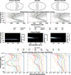 |
Fig. A.1 The inputs used to create the self-consistent spectra with PICASO for each atmospheric segment (top row). The second row shows the temperature-pressure profiles of each segment with the solid line indicating the original profile and the shaded regions the one and two sigma errors. The dash line indicates the modification to the profile for the isothermal models. The dotted lines are the condensation curves for different cloud species. Previous works have favoured the presence of Mg2SiO4 and MgSiO3 clouds over those of other types (Hoyer et al. 2023; Radica et al. 2024; Coulombe et al. 2025; Radica et al. 2025) thus we only consider Mg2SiO4 and MgSiO3 clouds in our models. The third row shows the optical depth per atmospheric layer of the modelled Mg2SiO4 and MgSiO3 clouds as a function of wavelength. In the eastern dayside model, the top of the cloud deck forms at 10−1∙5 bar and for the other two segments it is at 10−4 bar. The last row shows the VMRs of all the species used in these models for 10 times solar metallicity. These assume equilibrium chemistry with the original temperature profile (solid lines) and modified profile (dashed lines). |
All Tables
Previously derived orbit parameters for LTT-9779 b along with those derived in this work.
All Figures
|
Fig. 1 Spectrum of a hydrogen-helium atmosphere with a uniform volume-mixing ratio of Fe of 0.0001 (see Sect. 5.2.2). Each line represents a model with a grey cloud deck at a different altitude. This is represented by the cloud top pressure. |
| In the text | |
|
Fig. 2 Top panel: phase-folded radial velocity curve comprised of radial velocity measurements from this work (ESPRESSO eclipse), ESPRESSO transit observations, and HARPS. The vertical extent of each point represents the error. For the radial velocities to appear as a continuous curve, the systemic velocity and the fitted instrumental offset were subtracted. Bottom panel: phase-folded short-cadence TESS light curve (light points). The darker points show a binned version of the curve. In both panels, the best-fit curve for a circular orbit is shown (orange). |
| In the text | |
|
Fig. 3 Phases of LTT-9779 b, assuming the ephemeris from the circular orbit fit in Table 3, covered by these observations. Each circle represents an exposure, and the shaded area indicates the secondary eclipse of the planet. The gaps in the observations taken on night 1 were due to technical difficulties, and the observations in night 3 were halted early due to precipitation. |
| In the text | |
|
Fig. 4 Schematic of the data reduction process for the spectral time series of order 76 in night 2. Each of the six top panels shows the time series of spectra. Each row represents one spectrum in the series. Top panel: original spectra. Second panel from the top: spectral time series after continuum normalisation. Third panel from the top: spectral time series after the mean spectrum was subtracted. Panels 4-6 from the top: Spectral time series after one, two, and three sysrem iterations were run on the time series. Bottom panel: difference in the standard deviation of the residuals between consecutive sysrem iterations as a function of the number of sysrem components. The shaded region highlights the one-sigma deviation in the last four points (to the right of the dashed line), and the black dot indicates the chosen number of iterations (the smaller number), as described in the text. |
| In the text | |
|
Fig. 5 High spectral resolution (R = 70000) models computed using the eastern dayside, dayside, and western dayside mean temperature profiles from Coulombe et al. (2025, T.1) assuming 10 times solar metallicity. Each panel shows two spectra, one spectrum that assumes equilibrium chemistry for all species (Ch. 1,) and another that removes TiO from the atmosphere (Ch. 2). The contrast ratio measured by Coulombe et al. (2025, see Fig. 3 of their work) for each segment is shown as the dashed line, and the shaded region indicates the one-sigma errors. |
| In the text | |
|
Fig. 6 Vyys-Kp maps for the self-consistent 100 times solar dayside model for the original temperature profile (T.1). Left panel: Vsys-Kp map in terms of the S/Np computed from the cross-correlation coefficients. Right panel: Vsys-Kp map in terms of the significance computed from the likelihood (see Sect. 5.4). Neither map shows a significant peak at the known orbital parameters of the planet (Vsys = 0kms−1, Kp = 224kms−1), indicated by the crosshairs. |
| In the text | |
|
Fig. 7 Top left panel: Vsys-Kp map for for the single-species Fe model with a VMR of 0.01 and a cloud top pressure of 10−1∙5 bar for all post-eclipse data containing a significant false-positive signal. The red crosshairs indicate the expected location of the planetary signal. The remaining three panels show the corresponding maps for each of the observing nights individually. There is no map for night 3 as no posteclipse data were taken. |
| In the text | |
|
Fig. 8 Example of an injection-recovery test. Top panel: Vsys-Kp map when the true observations are compared to the self-consistent 100 times solar western dayside model with the original temperature profile. Bottom panel: Vsys-Kp map when the same model was injected into the data at a negative orbital velocity (reversed y -axis). The expected location of the signal is indicated by the crosshairs in both panels. |
| In the text | |
|
Fig. 9 Results of the injection-recovery test on the self-consistent models with the original temperature profile (T.1 in Table 4). The black square indicates that the highest likelihood peak exceeded 50kms−1 in Vsys or Kp from the expected location of the injected orbit. The coloured squares indicate the significance (∆σ) at which the injected spectrum was recovered. The grey squares indicate the models that were recovered at ∆σ < 5. |
| In the text | |
|
Fig. 10 Same as Fig. 9, but for models created with the modified isothermal temperature profile (T.2 in Table 4). |
| In the text | |
|
Fig. 11 Significance, ∆σ, at which the model is recovered in the injection-recovery test on the single-species models for the post-eclipse observations. The black square indicates that the model was not recovered in the injection-recovery tests. The coloured squares indicate the significance at which the injected spectrum was recovered. The grey squares indicate the models that were recovered at ∆σ < 5. |
| In the text | |
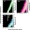 |
Fig. 12 Same as Fig. 11, but for the pre-eclipse observations. |
| In the text | |
|
Fig. 13 Restrictions placed on the vMR as a function of cloud deck altitude for the post-eclipse observations. The injection-recovery tests presented here rule out the models in light brown. Additionally, we highlight the models in dark brown which, due to the saturation of a large number of the spectral lines, have an average contrast ratio more than three sigma below the contrast of LTT-9779 b at these wavelengths measured by JWST NIRISS/SOSS data. To compare these restrictions to more complex models, we also plot the EUVMRS for metallicities ranging from 0.1 times solar to 1000 times solar as a function of the altitude of the cloud deck for the original (T.1, circles) and modified (T.2, crosses) temperature profiles for the western dayside. |
| In the text | |
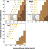 |
Fig. 14 Same as Fig. 13, but for the pre-eclipse observations and eastern dayside EUVMRS. |
| In the text | |
|
Fig. A.1 The inputs used to create the self-consistent spectra with PICASO for each atmospheric segment (top row). The second row shows the temperature-pressure profiles of each segment with the solid line indicating the original profile and the shaded regions the one and two sigma errors. The dash line indicates the modification to the profile for the isothermal models. The dotted lines are the condensation curves for different cloud species. Previous works have favoured the presence of Mg2SiO4 and MgSiO3 clouds over those of other types (Hoyer et al. 2023; Radica et al. 2024; Coulombe et al. 2025; Radica et al. 2025) thus we only consider Mg2SiO4 and MgSiO3 clouds in our models. The third row shows the optical depth per atmospheric layer of the modelled Mg2SiO4 and MgSiO3 clouds as a function of wavelength. In the eastern dayside model, the top of the cloud deck forms at 10−1∙5 bar and for the other two segments it is at 10−4 bar. The last row shows the VMRs of all the species used in these models for 10 times solar metallicity. These assume equilibrium chemistry with the original temperature profile (solid lines) and modified profile (dashed lines). |
| In the text | |
Current usage metrics show cumulative count of Article Views (full-text article views including HTML views, PDF and ePub downloads, according to the available data) and Abstracts Views on Vision4Press platform.
Data correspond to usage on the plateform after 2015. The current usage metrics is available 48-96 hours after online publication and is updated daily on week days.
Initial download of the metrics may take a while.