| Issue |
A&A
Volume 706, February 2026
|
|
|---|---|---|
| Article Number | A70 | |
| Number of page(s) | 15 | |
| Section | The Sun and the Heliosphere | |
| DOI | https://doi.org/10.1051/0004-6361/202453463 | |
| Published online | 02 February 2026 | |
Velocity field of an active region filament from GRIS infrared He I and IRIS ultraviolet observations
1
INAF – Osservatorio Astronomico di Roma Via Frascati 33 I-00078 Monteporzio Catone Rome, Italy
2
Space Science Data Center (SSDC), Agenzia Spaziale Italiana Via del Politecnico s.n.c. I-00133 Roma, Italy
3
INAF – Osservatorio Astronomico di Capodimonte Salita Moiarello 16 I- 80131 Napoli, Italy
4
Institut d’Astrophysique Spatiale, Bâtiment 121, Rue Jean Dominique Cassini, Université Paris Saclay 91405 Orsay, France
5
Instituto de Astrofísica de Canarias (IAC), Vía Láctea s/n E-38205 La Laguna Tenerife, Spain
6
Departamento de Astrofísica, Universidad de La Laguna, E-38206 La Laguna Tenerife, Spain
7
Institut für Sonnenphysik (KIS) Georges-Köhler-Allee 401a 79110 Freiburg, Germany
8
INAF – Osservatorio Astrofisico di Catania Via Santa Sofia 78 I-95123 Catania, Italy
★ Corresponding author: This email address is being protected from spambots. You need JavaScript enabled to view it.
Received:
16
December
2024
Accepted:
27
October
2025
Abstract
Context. Plasma flow measurements in solar active region filaments are rare, particularly in the infrared and ultraviolet ranges that probe the chromosphere and transition region. In addition, previous studies generally focused on prominences and filaments near the solar limb.
Aims. This study presents a multi-wavelength, multi-instrument analysis of an active region filament observed on the solar disk on November 9 and 10, 2020. Our goal is to characterize the plasma flows in the filament using spectroscopic measurements in both the infrared and ultraviolet spectral ranges. This is important for understanding the mechanisms for filament support, mass loading, and energy balance. Furthermore, this also offers observational benchmarks for filament modeling and simulations.
Methods. Spectra from the IRIS satellite, including the Mg II k 2796 Å, C II 1335 Å, and Si IV 1393 Å lines were analyzed alongside ground-based observations from the GREGOR Infrared Spectrograph and High-resolution Fast Imager instruments, whose observed spectral ranges include the chromospheric He I 10830 Å and Hα 6563 Å lines.
Results. Persistent blueshifts were measured within the filament structure in both spectral ranges. These can be interpreted as upflow velocities ranging from 0.5 to 15 km s−1, with Si IV 1393 Å showing the highest values. Redshifted emission in He I and Mg II k3 at the footpoints of a newly formed dark bundle suggest chromospheric downflows, likely due to spatial overlap between an arch filament system close to the filament footpoints. The weak redshifted signal in the Si IV emission may suggest confinement to lower atmospheric layers.
Conclusions. The observed velocity patterns provide, for the first time, a comprehensive and coherent view of the plasma dynamics from the chromosphere to the transition region, illustrating that the filament emission is consistently blueshifted in all the spectral windows, and thus in different temperature regimes.
Key words: Sun: chromosphere / Sun: evolution / Sun: filaments / prominences / Sun: infrared / Sun: transition region / Sun: UV radiation
© The Authors 2026
 Open Access article, published by EDP Sciences, under the terms of the Creative Commons Attribution License (https://creativecommons.org/licenses/by/4.0), which permits unrestricted use, distribution, and reproduction in any medium, provided the original work is properly cited.
This article is published in open access under the Subscribe to Open model. This email address is being protected from spambots. You need JavaScript enabled to view it. to support open access publication.
1. Introduction
Filaments and prominences are cool, dense structures of chromospheric plasma suspended in the corona above polarity inversion lines (PILs) in the photospheric magnetic field (Parenti 2014). These structures are referred to as filaments when observed on the solar disk, and as prominences when seen off-limb. They are observed both in active regions (ARs) and in the quiet Sun, where they are referred to as AR and quiescent filaments, respectively. AR filaments are typically more dynamic, smaller in size, and short-lived compared to their quiescent counterparts. Both quiescent and AR filaments form within so-called filament channels, which appear as long, narrow structures characterized by a pattern of fibrils along the PILs. During the formation process, these fibrils gradually reorient from a perpendicular to a parallel alignment with respect to the PIL, over a timescale ranging from three hours to one or two days (Gaizauskas et al. 1997; Wang & Muglach 2007).
Filament (and prominence) plasmas have temperatures below 106 K, and they are embedded in hotter coronal plasma. The interface between the prominence and the corona is known as the prominence-corona transition region (PCTR). This is defined as the region where the plasma temperature rises from about 7000 K to 106 K in analogy to the transition region between the chromosphere and the corona. Different diagnostic tools are employed to study the two components of a filament: the cooler core and the PCTR. The former is investigated through hydrogen and helium spectral and continuum emissions. The latter, instead, is analyzed by observing transition region spectral lines. As in the filament core, the PCTR is also characterized of a variety of flows, which are best measured in the ultraviolet (UV) and extreme UV spectral ranges.
Filamentary-like structures are also observed in emerging flux regions, which often display so-called arch filament systems (AFSs; e.g., Bruzek 1967, 1969). These structures consist of magnetic loops filled with cool plasma connecting opposite emerging polarities (Solanki et al. 2003). They are typically observed in chromospheric lines such as Hα, Ca II infrared, Ca II H & K, and He I 10830 Å (e.g., Spadaro et al. 2004; Zuccarello et al. 2005; Murabito et al. 2017; González Manrique et al. 2018, 2020; Joshi et al. 2024), and they exhibit upflows at loop tops and downflows at the footpoints of several tens of km s−1 (Balthasar et al. 2016; Zhong et al. 2019). Quiescent and AR filaments, instead, are characterized by different kinds of flows. This has implications in our understanding the mechanism of formation and their stability (Parenti 2014). However, measurements of plasma flows in filaments are limited, and most of the available observations focus on quiescent filaments.
A few studies investigated AR filaments. For instance, using infrared (IR) photospheric Si I and chromospheric He I spectral lines, Kuckein et al. (2012) reported small photospheric upflows of about −0.15 km s−1 under an AR filament. The chromospheric portion of the same filament showed an average upward motion of −0.24 km s−1. Hα observations reported by Ioshpa & Obridko (1999) show that AR filaments are located above regions characterized by chromospheric upflow motions, surrounded by areas of downflow motion. This property is shared with quiescent filaments.
Until the launch of the Interface Region Imaging Spectrograph (IRIS, De Pontieu et al. 2014), most observations of filaments in the UV range had been obtained with the Ultraviolet Spectrograph and Polarimeter (UVSP) instrument on the Solar Maximum Mission (SMM, Woodgate et al. 1980) first, and later with the Solar Ultraviolet Measurements of Emitted Radiation (SUMER, Wilhelm et al. 1995) instrument aboard SOHO. These earlier studies outlined the key findings listed below.
-
(i)
Persistent upflows of 5.6 km s−1 were observed at the filament locations using the SMM C IV 1548 Å line, which formed in the PCTR at 105 K (Schmieder et al. 1984).
-
(ii)
A transition between redshifts and blueshifts was detected on either side of the filament using the SMM C IV 1548 Å and Si IV 1393 Å spectral lines (Engvold et al. 1985). These results are consistent with the findings of Ioshpa & Obridko (1999). Engvold et al. (1985) also reported a velocity amplitude of ±15 km s−1 for both quiescent and AR filaments.
-
(iii)
Redshifted brighter areas, interpreted as being near the filament footpoints, were reported using Si IV SUMER data, although no clear velocity signature was associated with the filament (Kucera et al. 1999).
Doppler line shifts and the corresponding line-of-sight (LoS) velocities are affected by various sources of uncertainty. The inferred velocity values are position-dependent on the solar disk, and most of the reported measurements refer to filaments approaching the limb. This makes it difficult to make a direct comparison, as photospheric lines typically exhibit much smaller velocity shifts compared to those in the chromosphere or PCTR. A reliable zero-reference for the rest wavelength is ideally obtained using photospheric lines. However, such lines are rarely detectable in the UV spectral range. Therefore, setting an accurate zero-reference wavelength is necessary.
Several studies have reported difficulties in achieving absolute wavelength calibration (e.g., Engvold et al. 1985; Kucera et al. 1999). In the literature, velocity estimates are often derived under certain assumptions, such as averaging the wavelength over a full raster scan (Brooks & Warren 2009) or using quiet Sun (QS) regions far from the target as a reference (Del Zanna & Bradshaw 2009). These methods generally result in uncertainties greater than 5 km s−1 (Winebarger et al. 2013). A more accurate approach, though only feasible in the presence of two or more telluric lines has been used by Martínez Pillet et al. (1997) and Kuckein et al. (2012). As discussed in Section 3.2, this method achieves an uncertainty of less than 0.06 km s−1.
Given the observational issues described above, simultaneous high-spectral and high-spatial resolution measurements of plasma flows in filaments, at various wavelengths, sampling different atmospheric layers, remain relatively rare. In this study, we present a multi-wavelength analysis of the velocity field in an AR filament, tracing plasma motions from the chromosphere up to the transition region. We used the most accurate velocity calibration to date for the employed spectral ranges.
2. Observations
The AR filament analyzed in this study was observed on 2020 November 9 and 10 with the 1.5-meter GREGOR solar telescope (Schmidt et al. 2012; Kleint et al. 2020) located on Tenerife, Spain, during an observing campaign supported by the SOLARNET Transnational Access and Service Programme. The target (shown in the full-disk image of Fig. 1A) was AR NOAA 12781, which exhibited a βγ magnetic configuration consisting of a large sunspot in the leading negative polarity, an orphan penumbra, and several small pores in the following positive polarity (see Fig. 1G). On November 9 and 10, the AR was located at solar heliocentric coordinates [X, Y]=[140″, −431″] and [250″, 427″], respectively. Figure 1 (panels B-G) displays the filament and its surrounding environment in AIA/SDO, HiFI/GREGOR, and IRIS data. The filament is easily distinguishable in panels B, C, D, and E as a compact and dark structure located between two AFSs, connecting the two opposite polarities seen in the magnetograms to the north and to the south of the filament itself. Surrounding the filament, particularly on its western side, intense activity is visible in terms of brightening events at chromospheric and coronal heights (Fig. 1B and C). In contrast, the UV Mg II k3 intensity (Fig. 1 panel E) does not show any significant brightness enhancement in the same area.
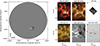 |
Fig. 1. Overall view of AR12871. Panel A: Full-disk magnetogram clipped between ±500 G from HMI taken at 10:55 UT on November 10. The black box indicates the FoV shown in the following AIA 304 and 193 Å bands (panels B and C). Panel D: High-spatial resolution HiFI Hα image taken at 10:48 UT on November 10. Panel E: IRIS slit-reconstructed image in the center of the Mg II k3 line acquired between 11:03 UT and 11:52 UT on November 10. Panels F-G: HMI magnetogram clipped between ±500 G and continuum taken at 10:55 UT. The red box in the continuum image indicates the GRIS FoV. |
The GREGOR observations consisted of full-Stokes spectropolarimetric data obtained with the GREGOR Infrared Spectrograph (GRIS, Collados et al. 2012) and of fast-imaging data obtained with the High-resolution Fast Imager (HiFI, Kuckein et al. 2017; Denker et al. 2023). The adaptive optics system (Berkefeld et al. 2012) was used to minimize the image degradation due to seeing effects. Several spectropolarimetric maps were taken on November 9 and 10. Here, we only used the scans acquired on November 10 between 09:17:32 and 09:37:05 UT, when the slit was aligned with the filament, and scanned a large area of 56.3″ × 10.4″. The spectral region observed with GRIS comprises the photospheric Si I 10 827 Å and Ca I 10 839 Å lines, as well as the chromospheric He I 10 830 Å triplet, among other weaker lines. The step size of the slit was 0 13, and each step consisted of ten accumulations with an exposure time of 100 ms each. The spatial sampling along the slit was 0
 13. The field of view (FoV) is shown in Fig. 1 (panel G). A spatial scan consists of 200 steps in total, scanned in about 20 minutes. In addition, the HiFI instrument recorded images of the target using two synchronized cameras, one observing the Hα line core (Fig. 1D) and the other the continuum close to Hα. These data were recorded in bursts of 500 images with a frame rate of 99 Hz, from 08:44 UT to 11:02 UT on November 9 and from 08:44 UT to 10:49 UT on November 10 under good seeing conditions.
The He I 10 830 Å line is a widely used diagnostic of the chromosphere and transition region; it is sensitive to plasma dynamics across a range of temperatures, from the cool core of prominences and filaments to their PCTR. Its formation involves a complex interplay between photoionization-recombination processes, collisional excitation, and scattering of photospheric radiation by helium atoms in the metastable triplet state (1s2s3S). The line consists of three components, with rest wavelengths at 10 830.34 Å, 10 830.25 Å, and 10 829.09 Å. Unlike UV lines, these spectra can be reliably wavelength calibrated, making He I 10 830 Å a valuable reference for absolute velocity measurements.
We complemented the study using the Atmospheric Imaging Assembly (AIA, Lemen 2012) and the Helioseismic and Magnetic Imager (HMI, Scherrer et al. 2012) continuum filtergrams and magnetograms aboard the Solar Dynamics Observatory (SDO, Pesnell et al. 2012). The HMI continuum filtergrams and magnetograms were used to align all available data and locate the position of the filament with respect to the underlying photospheric magnetic field, while the AIA at 304 and 193 Å images were used to study the upper atmospheric response. The region of interest (RoI) was also observed by IRIS with many different observing modes and at many times during its passage across the disk (see, e.g., Fig. 1E). The different observing modes mainly concern the size of the area scanned from the slit. We analyzed the spectra taken during three time intervals with the same observing mode: a dense 320-step raster that lasted approximately 50–60 minutes between November 9 and November 10, as reported in Table 1. All data analyzed in this work are listed in Table 1.
Set of observations from different telescopes used in this study.
3. Data processing
3.1. Fast imaging data
The standard image-reduction steps were performed using the pipeline sTools (Kuckein et al. 2017), which includes dark-current and flat-field corrections, as well as image selection and alignment between the two cameras. The Hα and Hα-continuum pairs of images were used for image restoration using the Multi-Object Multi-Frame Blind Deconvolution technique (MOMFBD, Van Noort et al. 2005). The best 50 frames of each burst were sufficient to obtain one restored image, covering a region of about 64″ × 40″, or 1336 × 1016 pixels, with an image scale of 0 048/pixel.
3.2. He 10830 Å and Si 10827 Å
Dark and flat-field corrections, as well as polarimetric calibration, were applied to the GRIS data using the standard on-site data-reduction pipeline (Collados 1999, 2003). The GREGOR polarimetric unit was used for the polarimetric calibration (Hofmann et al. 2012). The Stokes profiles were normalized to the mean continuum, calculated from various QS areas within the FoV, excluding regions displaying notable polarization signal. An absolute wavelength calibration was possible using the two telluric H2O lines within the observed spectral range. The obtained wavelength vector was corrected for Earth’s orbital motions, solar rotation, and gravitational redshift; and it spanned between 10 823.3 and 10 841.4 Å (for more details, see Kuckein et al. 2012). The He I line-core slit-reconstructed image was obtained by calculating the minimum of the intensity within the He I spectral window.
The HAnle and ZEeman Light v2.0 code (HAZEL2, Asensio Ramos et al. 2008)1 was utilized to perform inversions on the He I triplet, as well as on Si I and telluric lines. By simultaneously inverting these nearby lines, we can account for their wing overlaps caused by the close proximity of the Si I line to the He I triplet. Although the results for the Si I line in the photosphere are not shown here, this process ensures a comprehensive approach. HAZEL2 is designed to incorporate various effects on the He I triplet, including atomic level polarization and Paschen-Back, Hanle, and Zeeman effects. In parallel, the Si I line inversion is executed using the Stokes Inversion based on Response functions (SIR) code (Ruiz Cobo & del Toro Iniesta 1992), while the telluric line was fit separately with a Voigt profile. The data derived from HAZEL2 ultimately provide insights into both the photosphere, derived from the Si I 10 827 Å line, and the chromosphere, from the He I 10 830 Å line.
For the He I triplet inversion, HAZEL2 assumes a cloud-model configuration, where the atmospheric parameters are kept constant within a slab located above the solar surface. The Stokes profiles for each pixel were fit using a model with two components: one reflects the derived atmosphere, while the other represents stray light. A consistent stray-light profile was used across all spatial locations and times in the temporal series obtained as an average over a QS area near the observed pores. The Doppler velocity from the He I triplet presented in this study was computed by inverting the full Stokes spectra with HAZEL2.
3.3. UV IRIS data
The IRIS data were reduced and calibrated using the Solar Software (SSW) packages. These account for geometrical, flat-field, and dark-current effects and for the orbital variation of the wavelength array as described in Wülser et al. (2018). Furthermore, we used all the spectral lines in the NUV spectra to check the absolute wavelength calibration.
We focused on the analysis of observations in the Mg II (log10T = 4.15 K), C II 1335 Å (log10T = 4.4 K), and Si IV doublet Å (log10T = 4.9 K) spectral lines. These cover from the upper photosphere to the transition region, respectively (Rathore et al. 2015; Dufresne et al. 2021).
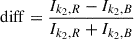
We derived the most used spectral characteristics from the Mg II lines, namely the k1 (h1), k2 (h2), and k3 (h3) features (Leenaarts et al. 2013). These were extracted from the spectra using the automated procedure iris_get_mg_features_lev2 available in the SSW IRIS package, which is described in Pereira et al. (2013). The error estimated for the k3/h3 Doppler velocity is the spectral sampling itself (0.05 Å). Here, we report the intensity and Doppler velocity of the line core for the Mg II k spectral line only, since the Mg II h line behaves similarly. Then, we used these quantities to estimate the k2 peak difference (diff), k2 peak separation (sep) – which are sensitive to the upper chromospheric velocity gradient (Leenaarts et al. 2013) – and the k2 peak asymmetry (asym), which gives the sign of the velocity above the τ = 1 level. The method to derive the diff, sep, and asym quantities is explained in Appendix A.
We performed an absolute wavelength calibration for the Si IV and C II spectral lines. From the calibrated spectra, we derived the peak intensity, Doppler velocity, and full width at half maximum (FWHM) for the Si IV and C II 1335 Å lines. For both lines, we performed a single-Gaussian fit using the curvefit.pro routine from IDL. We discarded pixels whose peak intensities were lower than 30 counts from the calculation. In addition, we also restricted the computation to profiles that have spectral widths larger than 70 mÅ. In the case of Si IV, we only show these calculated quantities for the Si IV 1393 Å component. Regarding the Si IV velocity, the associated uncertainty is 1.1 km s−1, as detailed in Appendix B. For QS regions, we find an average velocity value of 5.4 ± 0.6 km s−1, which is slightly lower than values reported in earlier studies such as Chae et al. (1998), Teriaca et al. (1999), and Peter & Judge (1999). All the details can be found in Appendix B.
For C II 1335 Å, although line profiles may exhibit single or double peaks due to temperature gradients between the chromosphere and the transition region (Rathore et al. 2015), we adopted a single-Gaussian fit for consistency, following similar approaches from previous studies (e.g., Upendran & Tripathi 2021). This choice is based on multiple tests, which showed that in cases where a double-Gaussian fit is feasible, the resulting difference in velocity does not exceed 30%. However, due to the generally noisy profiles and the estimated uncertainty of 3.3 km s−1 (see Appendix B), we consider the C II Doppler velocities as qualitative indicators only.
3.4. Co-alignment
The alignment of all the available observations required several steps. In particular, HMI continuum images taken at the same time as the ground-based observations were used as a reference to scrutinize the magnetic polarities, with an accuracy of 0.5″. These were also used to align the Hα broad- and narrow-band images. A finer alignment was necessary for all ground-based Hα images, which were interpolated to have a common FoV and a common spatial scale. Then, the high-resolution Hα image at 10:48 UT on November 10 was used as a reference to co-align the UV IRIS line observations. This choice reflects the almost co-temporal time acquisition of the ground-based measurements and IRIS second scan. Finally, using the broad-band images (closest in time), we aligned the GRIS data.
4. Results
4.1. Hα filament fine structure
Figure 2 displays the restored Hα filtegrams acquired by the HiFI instrument and shows the fine structure of the filament at various times on November 9 and 10 (top and bottom panels, respectively). The filament is approximately 5″ wide and longer than 50″ (see the maps shown in Fig. 2). In particular, the first maps on November 9 and 10 (first column of Fig. 2) show the contours of locations of positive and negative magnetic fields from HMI data, marked in red and blue, respectively. On both days, the filament is located above the main PIL of the AR. The red box in the second-from-bottom panel displays the area scanned by GRIS that covers the filament. A closer inspection of the top panels in Fig. 2 for November 9 reveals a system of threads that is less compact on the northern side than the southern one. This effect could be ascribed to the viewing angle of the structure. The filament appears progressively darker and more compact with time (see the online movies). Furthermore, on November 10 it is surrounded by active areas, which are seen as bright in the Hα images. The filament appears to be composed of more than two systems. A new, darker, and more compact bundle emerges in the northern part. In particular, by comparing the IRIS Mg II k3, AIA 304 Å, and AIA 193 Å maps (panels B, C, and E in Fig. 1) it is possible to note that this latter bundle, which becomes darker and more compact in Hα, does not seem to belong to the northern AFS, but rather resembles a continuation of the central filament. This interpretation is further supported by the magnetic configuration shown in panel F in Fig. 1. From visual inspection, between November 9 and 10 (see Fig. 2, top panels to bottom panels, and the online movies) the thread orientation changes in a clockwise direction. However, this does not occur uniformly along the entire length of the filament. As generally expected at AFS footpoints, where velocities decrease (redshifted) and then accelerate to supersonic speeds, generating shocks and heating the surrounding atmosphere and higher layers, two homologous brightening events are detected at the edge of the northern AFS and on the western side of the filament at 08:49 UT and 09:19 UT on November 10 (see the first two bottom panels of Fig. 2 and the online movie).
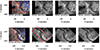 |
Fig. 2. Restored Hα filtergrams acquired by HiFI instrument at GREGOR telescope showing fine structure of filament at various times on November 9 (top panels) and November 10 (bottom panels). The red and blue contours in the first panels indicate the positive and negative magnetic flux density obtained from SDO/HMI at level equal to ±200 G, respectively. The red box in the second-from-bottom panel represents the GRIS acquired scanned FoV from between 09:17:32 and 09:37:05 UT. Movies of the HiFI data showing the filament in the time interval between 08:44 UT and 11:02 UT (10:49 UT) on November 9 and 10 are available online. |
4.2. He I observation
Figure 3 displays the slit-reconstructed line-core intensity map of the He I line (middle panel), and the corresponding Hα image for a comparison (top panel). The He I line-core intensity map shows a portion of the filament, outlined by the red box in Fig. 2, as a thin, dark, and elongated structure extending from 0 to 30″ in the x direction. Additionally, there are a series of thin threads marked by the white arrows from 25″ to 40″ (x direction). Interestingly, the filament does not appear as a dark, continuous structure along its full length in He I 10 830 Å, unlike in Hα observations. This may reflect variations in the PCTR across different segments of the filament, differences in the local EUV illumination – which we cannot directly measure – or a combination of both effects. These variations in He I absorption may also correspond to the two filament segments discussed in the Hα section, although this requires further verification. Red, blue, and orange crosses, labeled as 1, 2, and 3, are marked on the He I line-core intensity map to indicate specific pixels belonging to the QS (label 3), and to dark and bright regions within the filament (labels 1 and 2, respectively). The spectral profiles for each of these positions, within the He I spectral window, are shown in the bottom panel of Fig. 3. The normalized spectrum shows that the absorption profile in the central bright part of the filament (blue profile labeled “2” in the middle panel) is significantly shallower, with an intensity reduction of about 30% compared to the darkest region (red profile). This shallower profile is more similar to that observed in the QS (orange profile). This peculiarity could be ascribed to specific mechanisms of He I triplet line formation, which is influenced by both EUV illumination from the surrounding corona and the presence of the filament PCTR, as discussed by Andretta & Jones (1997), Labrosse et al. (2002) and Labrosse & Gouttebroze (2004). Moreover, thin, elongated, darker threads are visible in the central portion of the filament in the He I line-core intensity map (see white arrows in Fig. 2).
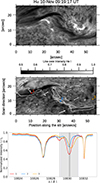 |
Fig. 3. Top panel: Zoomed-in view of Hα filtergram for reference. Middle panel: GRIS slit-reconstructed He I line core intensity of the RoI acquired between 09:17:32 and 09:37:05 UT on November 10. Bottom panel: Stokes-I profiles, normalized to continuum intensity, observed at the red, blue, and orange (1, 2, and 3) positions shown in the He I line core map. Arrows point to thin, darker, elongated threads where the optical thickness of the He I line is higher than their own surroundings (Fig. 4). White contours represent a plasma velocity of about −1 km s−1. The shaded area indicates where the He I line core is calculated (see Sect. 3.2 for more details). The vertical lines represent the rest wavelengths for the three He I components as reported in Table 1 of Kuckein et al. (2012).
|
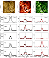 |
Fig. 5. From top to bottom: Peak-intensity maps and spectral profiles in locations marked with an asterisk in the respective intensity maps and their relative fits of Mg II k, Si IV 1394 Å, and C II 1335 Å during the middle IRIS raster scan (11:03–11:52 UT). Original spectral line profiles are shown in black and corresponding Gaussian fits are shown in red (for Si IV and C II spectral lines). |
Maps of Doppler velocity and the slab optical thickness2 of He I as retrieved by the HAZEL2 code are shown in Fig. 4. The Doppler-velocity map mainly displays two blueshifted areas in correspondence of the AR filament, while redshifted plasma is observed almost elsewhere. The darker and elongated part of the filament, as seen in the He I line core, corresponds to the new structure that previously appeared in Hα. This region displays both upward (between X coordinates from 0″ to 15″) and downward motions (between X coordinates from 10″ to 30″). In particular, the observed redshifted component reaches values exceeding 10 km s−1 (as indicated by the green and yellow contours, corresponding to velocities of 10 and 15 km s−1, respectively). This redshift may be associated with the footpoints of the northern AFS, and possibly also with those of the filament, suggesting a partial spatial overlap between the two structures in the chromosphere. The region characterized by a decrease in the He I absorption profile (see the blue profile in Fig. 2 bottom panel) displays upward motions reaching velocities up to −3.5 km s−1, with an average velocity of −1.9 km s−1 (within the black contour in Fig. 4). This area also exhibits a relatively low optical thickness, below 1 (see bottom panel of Fig. 4). Notably, darker, thin threads, indicated by the red (or white) arrows, are visible in the region and are associated with slightly higher optical thickness values, around 1, compared to their surroundings. In contrast, the darker, elongated structure has an optical thickness value ranging from 1 to 2.5, consistent with those reported by Díaz Baso et al. (2019).
4.3. UV IRIS observations
Figure 5 shows the IRIS peak-intensity maps within the RoI, acquired during the raster scan on November 10, between 11:03 UT and 11:52 UT. The maps correspond to the three brightest IRIS UV lines, ordered by increasing formation temperature: Mg II k3, C II 1336 Å, and Si IV 1393 Å. Spectral profiles at five representative pixel positions, marked with asterisks on the maps, are also shown. These pixels were selected to represent different spectral behaviors observed across the FoV. For both the C II and Si IV pixel profiles, single-Gaussian fits to the observed profiles are shown in red.
Within the filament, the Mg II k line profiles (e.g., at F1, F2, and F3) exhibit typical spectral features: two emission peaks (k2) separated by a central absorption dip (k3). In contrast, outside the filament, such as at the QS2 location, which belongs to a magnetized area due to the presence of a nearby pore and sunspot (see Fig. 1G), the profiles may lack the k2 peaks and appear fully in emission. While these differences do not affect the measurements of the k3 Doppler shift, they can influence other spectral diagnostics (see Fig. 10 and related discussion). As shown by Rathore et al. (2015), C II line profiles may exhibit either a single- or a double-peaked profile, depending on the variation of the source function and the presence of LoS velocity gradients. A central absorption dip forms when the source function decreases before the optical depth reaches unity. Velocity gradients can Doppler-shift the absorption profile, distorting symmetric double peaks into asymmetric single peaks. For a comprehensive discussion of C II line formation, we refer the reader to Rathore et al. (2015), Rathore et al. (2015) and Avrett et al. (2013). In our data, QS profiles are not uniformly single-peaked; for example, the QS2 profile is single-peaked, while the QS1 profile shows poorly defined peaks. In contrast, the filament profiles (F1, F2, and F3) consistently display double-peaked C II profiles.
The last column of Figure 5 presents the corresponding Si IV profiles at the five selected pixel positions. In all filament positions, the signal is well above the noise level, ensuring the robustness of the Gaussian fits and, consequently, the accuracy of the Doppler-shift estimates derived from the line centroid, given that the spectral profiles exhibit a clear Gaussian shape.
Figure 6 reports peak-intensity maps for the Mg II k, CII, and Si IV spectral lines for the entire FoV observed, respectively. Although the first IRIS raster scan was acquired approximately ten hours after the GREGOR high-resolution Hα observations, a comparison reveals that the morphology of the filament in the first Mg II k scan (acquired between 20:26 and 21:15 UT on November 9) is similar to that seen in the GREGOR Hα images (see bottom panels of Fig. 2) taken on November 10, 08:00 UT. Due to the spatial resolution of IRIS and the different formation heights of the spectral lines, the fine structure of the filament seen in the ground-based Hα observations is not resolved in the Mg II k peak intensity maps. Individual threads along the filament axis are distinguishable in the Mg II k peak intensity. Nonetheless, a filamentary but less compact structure, somewhat resembling that seen in Hα, can still be identified in the region X = [30″, 45″] and Y = [45″, 60″], as indicated by the two red arrows in the top left panel. This gap region shows localized brightening activity in both the C II and Si IV 1393 Å intensity maps. The latter (bottom left panel) also displays the presence of filamentary threads at the western edge of the gap, as well as within the central brightening area. Given the observable temporal changes, these features may indicate ongoing localized reconnection, where threads are changing from inclined to vertical configurations, which is consistent with the findings of Zhou et al. (2016).
The second IRIS scan was acquired just at the end of the Hα ground-based observations. In this case, the Mg II k and Hα images appear similar, both clearly showing barbs and fine threads along the filament. After about nine hours, during the third IRIS scan (taken between 20:48 and 21:37 UT; see top right panel) the filament structure seems to undergo structural changes. Rather than a continuous structure, the filament now appears as a bundle of filamentary threads, with a brighter area on its western side.
Even though the C II and Si IV maps are noisier than those in the Mg II k line, the filament remains well recognizable in the first two raster scans (first two middle and bottom panels of Fig. 6). However, at the eastern and western edges of the filament, the peak intensity of the C II 1336 Å cannot be reliably measured due to lower signal levels and the presence of more complex line profiles. The morphology of the filament on November 10 resembles that seen in the Hα observations, both in terms of length and dimension (see the white contour in the middle panel of Fig. 6). Brightening areas are visible at the edge of the filament, and the last scan (right middle panel of Fig. 6) clearly displays small-scale brightening events occurring within the filament.
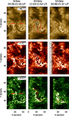 |
Fig. 6. Peak-radiance maps Mg II (top), C II (middle), and Si IV (bottom). These maps result from the three IRIS rasters reported in Table 1. Contours in all middle panels indicate the high-resolution GRIS Hα filament contour. The red boxes represent the three panels shown in Fig. 8. |
In contrast to previously reported SUMER observations in Si IV lines (Kucera et al. 1999), the filament is clearly detectable in the Si IV peak intensity during the first and second raster scans. Similarly to the C II maps, a localized bright region is observed surrounding the filament on its western side. The filament is still detectable under the Hα red contour at 11:02–11:52 UT on November 10. By the time of the final raster scan, this bright region has expanded, appearing to cover much of the filament. Furthermore, several elongated bright patches are observed between the threads, while only a small portion of darker filamentary structure is visible (see the red box in the bottom right panel of Fig. 6). These small-scale brightening events do not appear to be fully co-spatial with those seen in the C II data.
4.4. UV Doppler velocities and velocity gradients
Doppler-velocity maps for the three IRIS lines are displayed in Fig. 7. As in Fig. 6, the maps are organized from top to bottom by spectral line: Mg II k3, CII, and Si IV, respectively, for the three IRIS raster scans. In all panels, a smooth contour outlines the filament. This contour was defined by applying an intensity threshold to the Mg II k peak intensity line, and then it was cleaned up to highlight the filament structure as a whole.
In all maps, the filament is blueshifted. As has long been observed and described (Parenti 2014; González Manrique et al. 2018), a clear flow of material is present along the AFSs, moving from one footpoint to the other through the system of bundles. This feature becomes particularly evident during the last two scans (11:03–11:52 UT and 20:48–21:37 UT, shown in the middle and right panels of Fig. 7). The plasma patterns observed in the AFSs correspond closely to the representation given in Figure 15 of González Manrique et al. (2018) and have been observationally reported in González Manrique et al. (2020) and more recently in Joshi et al. (2024). Notably, in the middle raster scan, only the Mg II k3 Doppler-velocity map clearly reveals the presence of the redshifted area at the tail of the two filament sectors previously identified in Hα and He I images, with velocity exceeding 15 km s−1. Furthermore, these redshifted footpoints are barely visible in the Si IV map. This may suggest that the northern AFS has already risen to higher layers of the atmosphere. A similar behavior is shown in panel (e) of Figure 15 in González Manrique et al. (2018), where He I observations of their AFS exhibit gradually decreasing downflows at the footpoints. The three Doppler-velocity maps display a different range of values. In the Mg II k3 Doppler-velocity maps, the filament shows upward velocities in the range of [−0.5,−3] km s−1. The Si IV maps report relatively higher velocities in the filament, with values in the range of [−6,−15] km s−1. The C II Doppler-velocity maps are noisier compared to the other two UV maps. As a result, the velocity pattern within the AFS is less clear compared to the Mg II k3 and Si IV maps. The maps clearly show that inside the Mg II k3 contour, the plasma consistently exhibits blueshifts across all three datasets, indicating coherent upward motions in this region despite the increased noise in the C II observations.
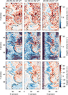 |
Fig. 7. Velocity maps for Mg II (top), C II (middle), and Si IV (bottom) observations. In all panels, black contour represents Mg II k3 intensity. |
By closely inspecting the IRIS Mg II k and Si IV peak intensity and velocity maps, we can compare the fine structure of the filament in these spectral lines and examine the relationship between intensity and Doppler velocity. Figure 8 displays zoomed-in views of three different images, which are outlined by red boxes in the Mg II k peak intensity map of Fig. 6, as seen in the Mg II k and Si IV 1393 Å peak intensity, along with the corresponding Hα sections for comparison. We note that the Hα image corresponds to the last available frame taken at 10:58 UT before the IRIS observation, while the IRIS rasters were acquired between 11:03 and 11:52 UT. Although the filament is clearly visible in the core intensity maps of both Mg II k and Si IV, its fine structure is better resolved in the Hα observations. Nevertheless, the figure provides useful insights into the spatial relationship between the filament intensity and the surrounding Doppler-velocity field. Indeed, Figure 9 shows the intensity and Doppler-velocity profiles along the black horizontal segment indicated in all panels of the middle row in Fig. 8. In this horizontal cut, a distinct drop in intensity marks the position of the filament. Blueshifted plasma is associated with this intensity dip, as is particularly evident in the Si IV data. Although the intensity decreases on both the eastern and western sides of the filament, it does not recover to pre-filament levels on the western side, suggesting additional structuring or obscuration. Moreover, positive Doppler velocities are observed just before the western edge of the filament, indicating localized downflows in that region. This effect may be related to the filament’s position on the solar disk. In addition, compared to previous figures, the Si IV maps more clearly highlight that the redshifted footpoint visible in the Mg II k3 velocity does not appear as prominently in the Si IV Doppler data, further supporting the idea that the downflow is confined to lower atmospheric layers.
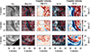 |
Fig. 8. Comparison of Hα and UV Mg II and Si IV IRIS intensity and Doppler velocity. From left to right: Hα intensity; Mg II k3 and Doppler velocity; Si IV peak intensity and Si IV Doppler-velocity maps for three RoIs (see the red boxes in the k3 intensity middle panels of Fig. 6). The Mg II k3 and Si IV Doppler-velocity maps are shown in the range from [−10, 10] to [−30,30] km s−1 as the original maps of Fig 10. In the Mg II k3 and Si IV intensity and Doppler-velocity maps, the red and blue contours represent upflows (−1 and −3 km s−1) and downflows (1 and 3 km s−1), respectively, corresponding to the Doppler velocities of Mg II k3 and Si IV. |
Figure 10 reports Mg II k2 peak-separation, difference, and asymmetry maps. These maps display patches of poor calculations on the eastern and western area at the edges of the filament due to single-peaked profiles (k2R or k2B not present, as already shown in the top right panel plot of Fig. 5). The filament displays a k2 peak separation that increases with time (see the top panels of Fig. 10). In the third IRIS scan, we observe a k2 peak separation larger than 30 km s−1 inside the filament. Concerning the k2 peak difference, shown in the second-row panels of Fig. 10, the filament is mainly characterized by a negative ratio, indicating stronger blue peaks corresponding to upflowing material above the Mg II k peak formation height. A positive ratio (with red peaks stronger than blue ones) appears to move along the length of the filament during the last two IRIS scans indicating downflowing material. Moreover, these last two scans display a higher concentration of Mg II profiles with positive k2 asymmetry (i.e., upflows) inside the filament k3 contour. Some patches of negative k2 asymmetry (i.e., downflows) are also visible.
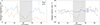 |
Fig. 9. Mg II and Si IV intensity and velocity variation along slit drawn in third middle panel of Fig. 8. The shaded area indicates the width of the filament as seen in the Mg II intensity maps. Error bars in the Si IV velocity plot were retrieved as explained in Sect. 3.3. |
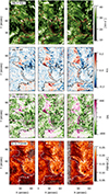 |
Fig. 10. From top to bottom: Mg II peak difference (diff), peak asymmetry (asym), peak separation (sep), and Si IV FWHM maps. Red and black contours indicate Mg II k peak intensity in all panels. |
The bottom panels of Fig. 10 display Si IV FWHM maps. On the western side of the FoV, we observe broader Si IV profiles and this characteristic increases with time, reaching a FWHM value of up to 0.25 Å in the third IRIS scan. As can be noted, this pattern seems to be persistent in time. The profiles appear to be broadened twice as much with respect to the eastern side. It can easily be possible to recognize three regions having different values of FWHM. In particular, the eastern side of the filament is characterized by a FWHM < 0.15 Å, while we find values between 0.1 and 0.2 Å inside the filament, and the values are greater than 0.2 Å on the western side of the filament. Knowing the IRIS instrumental and thermal broadening (see Del Zanna & Mason 2018), the FWHM for an optically thin line (as the Si IV) is related to the nonthermal velocity. Assuming a temperature formation of 80 × 103 K for the Si IV 1393.755 Å line, a thermal width of 6.88 km s−1, and the instrumental broadening equal to 3.9 km s−1 (De Pontieu et al. 2014), the filament has a nonthermal velocity between 13 km s−1 and 29 km s−1, while on the eastern and western sides of it we find values lower than 21 km s−1 and greater than 29 km s−1, respectively. The values reported for QS and AR areas using SUMER Si IV data are on the order of 27 km s−1, which are comparable to those found on the western side of the filament. For temperatures with log T < 5.4, as in the case of Si IV data, Parenti & Vial (2007) reported lower nonthermal-velocity values in prominences compared to those in the QS.
5. Discussion
In this paper, we present a multiwavelength, multi-instrument observation of an AR filament. These observations are especially noteworthy due to the combination of high-spatial-resolution Hα images and high-spectral-resolution He I data from the GREGOR telescope, complemented by near-simultaneous UV IRIS spectra and images sampling the solar chromosphere and transition region. This comprehensive dataset enabled us to investigate the filament’s fine structure and plasma dynamics in unprecedented detail.
The high-spatial-resolution Hα observations reported in this work reveal that the filament thickened over time (10:54 UT on November 9 and 10:48 UT on November 10), becoming darker and more compact. The fibril patterns became more pronounced (see the online movies and Fig. 3).
We observed a change in the orientation of the threads over a time span of almost 12 hours, which is consistent with the timescale reported in the literature. Although we observe Hα fibrils changing orientation, we do not capture, in this spectral range, any merging episodes or small-scale activity indicating interactions of threads and subsequent thickening of the filament. On November 10, Hα observations show that the filament appears darker and more compact compared to the previous day. A new darker and more compact structure also appears in the northern part of the FoV, resembling an extension of the filament. The simultaneous GRIS He I raster scan never clearly shows the presence of the main filament along its full length (Fig. 3), possibliy reflecting variations in the PCTR across different segments of the filament, differences in the local EUV illumination, or a combination of both effects. The helium core exhibits several thin threads in the region where Hα displays darker structures. Stokes-I profiles in the central part of the filament are shallower and reduced of over 30%. Furthermore, this central part has optical thickness values below unity compared to the darker part of the filament and the thin threads, whose values exceed 1.5 (Fig. 4). Small-scale brightening events are observed in the C II 1335 Å and Si IV 1393 Å peak-intensity maps. The presence of threads in between the observed brightening events may suggest possible thread formation or disappearance, as reported in Zhou et al. (2016).
As mentioned in Sect. 1, most studies of plasma flows in the UV range have focused on prominences or filaments observed near the limb. In contrast, our analysis concerns a filament located clearly on the solar disk, where projection effects are minimized (μ = 0.78–0.66). We report that the filament is consistently blueshifted in all the analyzed spectral lines (He I, Mg II k, C II, and Si IV) throughout the entire observation period. These blueshifts, interpreted in terms of upward velocities, highlight the presence of persistent upflows even in on-disk observations, as also reported in previous works (Schmieder et al. 1984; Kucera et al. 1999). Extending the study of Schmieder et al. (1984), where the authors reported blueshifts using Hα and the transition region C IV 1548 Å spectral lines on the order of [0.5, 5.6] km s−1, here we are able to infer Doppler velocities by using the IR He I 10830 Å and the three UV Mg II k, C II 1335 Å, and Si IV 1393 Å lines, all of them having persistent blueshift velocities on the order of [0.5, 15] km s−1. Noticeably, the IR He I and UV Mg II k3 Doppler-velocity maps highlight redshifted signatures at the end of the new dark and compact structure visible during the co-temporal ground-based and IRIS observations. This redshifted feature is barely visible in the Si IV map. The observed redshifted structure may be associated with the footpoints of the northern AFS and possibly also with those of the filament, reflecting an overlap between two structures in the chromosphere. This association can be seen in Fig. 11, which shows zoomed-in SDO/HMI and SDO/AIA 304 Å images. Indeed, the northern AFS displays a clear magnetic configuration in the SDO/HMI data, highlighting its connection between opposite polarities, while the filament is located along the PIL.
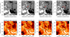 |
Fig. 11. SDO/HMI magnetograms (top panels) and SDO/AIA 304 Å images at four representative times. The black boxes indicate the magnetic configuration of the AFS. Magnetograms are clipped ±500 G. Red and black arrows point new magnetic features described in the text. |
Furthermore, in the images from 23:00 UT on November 9 (Fig. 11, see arrows), the new compact and darker structure, which is also visible in Hα and He I on November 10 (Fig. 8, top panels), displays the magnetic configuration of a filament, i.e., a feature along the PIL. This supports the probable coexistence of the northern AFS and of this new filament in the He I and Mg II k3 velocity maps. The reduced magnitude of the Si IV Doppler velocity may indicate that redshift signal relative to the northern AFS does not reach higher atmospheric layers. We recall that the estimated errors for the Si IV velocities are comparable with previous studies; they are of the order of 1 km s−1.
The study performed by Kucera et al. (1999) showed plasma upflows in the Hα observations acquired with the ground-based VTT telescope, but they could not detect any blueshift in the SUMER Si IV transition-region line. The Doppler velocity retrieved using the IR He I spectral line displays a clear blueshift velocity in the filament in the range of [0.5,3.5] km s−1, with an average Doppler velocity of −1.5 km s−1. The spectral range of He I 10 830 Å was used by Kuckein et al. (2012), which reported the study of Doppler velocities in an AR filament. In particular, that work found that the filament’s spine is dominated by upflow (reaching values of about −1 km s−1). On the contrary, the section of their filament observed above the orphan penumbra in the chromosphere appears to be redshifted, suggesting a different mechanism sustaining or creating the filament (from below the photosphere in their case). Díaz Baso et al. (2019) studied an AR filament located in a flaring area on chromospheric GRIS He I data, and reported upflow along the PIL on the order of −3 km s−1. Unlike previous studies that reported a mix of upflows and downflows in different parts of AR filaments, our observations reveal consistently blueshifted velocities along the filament, across all time windows and spectral ranges. While such differences may be due to variations in magnetic configuration, evolutionary stage, or observational setup, the coherence observed here could reflect the advantage of combining high-cadence, multiwavelength data over extended periods.
In addition, we reported the Mg II k2 separation, k2 difference and k2 asymmetry. These quantities are usually investigated in flare studies, such as in Polito et al. (2020), Polito et al. (2023a) and Polito et al. (2023b). Together with the Mg II k3 Doppler shift, these quantities are good diagnostics of plasma flow and velocity gradients in the solar chromosphere (Leenaarts et al. 2013). In our study, their values point to the presence of plasma flow and gradients along the full filament length. It is worth noting that the correlations shown in Leenaarts et al. (2013) and Pereira et al. (2013) have some spread, and they are valid for spectra at the disk center and cover QS conditions to which the simulation belongs. Since the IRIS launch, the Mg II h & k lines have also been modeled for different magnetic field topologies, such as those representative of the QS, ephemeral flux regions, and plages (Hansteen et al. 2023), as well as under various conditions such as flares (e.g., Kerr et al. 2016) and in prominence (Heinzel et al. 2014, 2015). Although these studies are not properly representative of our observations, the asymmetrical profiles of Mg II seem to be a result of fine unresolved plasma motion (Peat et al. 2023). Further dedicated numerical studies are needed to better understand the Mg II asymmetric profiles and the associated plasma dynamics in AR filaments, as well as their variation across the solar disk.
On both the eastern and western sides of the filament, but more clearly seen on the western side, a transition in plasma flow is evident; it is characterized by blueshifts within the filament and redshifts outside of it. This kind of behavior was previously pointed out by Engvold et al. (1985). AR filaments showing chromospheric upflows (using the IR He I spectral line) are embedded in a downflow area corresponding to the faculae region (Kuckein et al. 2012; Xu et al. 2012) and moss region (Zhao et al. 2024). Kuckein et al. (2012) speculated that such a downflow at the faculae region could probably be associated with coronal rains and/or their different manifestations (Lagg et al. 2007). The results presented in Zhao et al. (2024) display brightening events and apparent downflow in the moss region (footprints of 2-3 MK loops beneath the 1 MK loops).
Finally, the nonthermal velocities reported in our case are comparable with those found in QS and AR by Teriaca et al. (1999). All are lower than those in the QS inside the filament, as reported in Parenti & Vial (2007) in the temperature range analyzed (log T < 5.4).
6. Conclusion
In summary, our multiwavelength analysis provides a coherent view of the plasma dynamics in an AR filament, from the chromosphere to the transition region. By combining IR and UV Doppler diagnostics, we tracked persistent flow patterns over two consecutive days, revealing a stable velocity field across a wide range of temperatures.
Throughout the observing period, we consistently detected blueshifted velocities in the He I, Mg II k3, Si IV, and C II lines, indicating stable upflows from the chromosphere into the transition region. In contrast, redshifted features at the footpoints of a newly formed structure, clearly visible in the He I and Mg II lines, suggest chromospheric downflows possibly due to an overlap with an AFS. The absence of this signal in Si IV may point to its confinement to lower atmospheric layers. Additionally, asymmetries in the Mg II k2 support the presence of flows and velocity gradients along the entire filament spine.
Importantly, this work represents one of the very few studies to combine ground-based IR observations of He I 10 830 Å with UV-transition-region diagnostics (e.g., Mg II, Si IV, and C II) for an AR filament. While previous studies have primarily focused on quiescent filaments or prominences, often relying on indirect velocity measurements, our analysis directly captures dynamic behavior across multiple atmospheric layers with substantially improved resolution. In doing so, we confirm and extend early findings from missions such as SMM and SUMER, while addressing an area of solar physics that has remained relatively unexplored in the high-resolution era.
Despite known limitations in the IRIS dataset, our results present a consistent and robust picture of the filament dynamics across multiple layers of the solar atmosphere. This demonstrates the potential of coordinated IR and UV spectroscopy for studying fine-scale filament evolution and plasma motions. Future observational proposals could take advantage of the lessons learned from this study by integrating both high-resolution chromospheric observations from instruments such as CRISP (Scharmer et al. 2008), CHROMIS (Scharmer 2017), and GRIS and those available at the DKIST telescope, and coronal observations from Hinode/EIS (Culhane et al. 2007) and SO/SPICE (SPICE Consortium 2020). More systematic and continuous observational campaigns, targeting a filament over several days and utilizing complementary instruments capable of resolving both the plasma flows and magnetic field structures, would allow us to infer all relevant physical parameters such as mass density, temperature, velocity, and magnetic field. This approach could pave the way for future synergistic studies combining spectropolarimetric measurements from IBIS2.0 (Ermolli et al. 2020; Viavattene et al. 2022; Ermolli et al. 2024) in the photosphere and chromosphere with UV observations from Solar-C (Shimizu et al. 2019) and MUSE (De Pontieu et al. 2020; Cheung et al. 2022), offering a comprehensive understanding of the filament’s kinematic and magnetic properties.
Data availability
Movies associated with Figs. 2 are available at https://www.aanda.org
Acknowledgments
This research was supported from the European Union’s Horizon 2020 research and innovation programme under grant agreement no. 824135 (SOLARNET) and by the Italian Space Agency (ASI) under contract with the INAF no. 2021-12-HH.0 and Addendum 2021-12-HH.1-2024 “Missione Solar-C EUVST-Supporto scientifico di Fase B/C/D”, and under contract with the INAF no. 2022-29-HH.0 “Missione MUSE”. CK acknowledges grant RYC2022-037660-I and SJGM grant RYC2022-037565-I, both funded by MCIN/AEI/10.13039/501100011033 and by “ESF Investing in your future”. Financial support from grant PID2024-156538NB-I00, funded by MCIN/AEI/ 10.13039/501100011033 and by “ERDF A way of making Europe” is gratefully acknowledged by SJGM.” MM would like to thank Ilaria Ermolli and Roberto Piazzesi for their valuable discussions, insightful suggestions, and assistance with language editing, all of which contributed to improving the manuscript.
References
- Andretta, V., & Jones, H. P. 1997, ApJ, 489, 375 [NASA ADS] [CrossRef] [Google Scholar]
- Asensio Ramos, A., Trujillo Bueno, J., & Landi Degl’Innocenti, E. 2008, ApJ, 683, 1 [Google Scholar]
- Avrett, E., Landi, E., & McKillop, S. 2013, ApJ, 779, 155 [NASA ADS] [CrossRef] [Google Scholar]
- Balthasar, H., Gömöry, P., González Manrique, S. J., et al. 2016, Astron. Nachr., 337, 1050 [NASA ADS] [CrossRef] [Google Scholar]
- Berkefeld, T., Schmidt, D., Soltau, D., et al. 2012, Astron. Nachr., 333, 863 [NASA ADS] [CrossRef] [Google Scholar]
- Brooks, D. H., & Warren, H. P. 2009, ApJ, 703, L10 [Google Scholar]
- Bruzek, A. 1967, Sol. Phys., 2, 451 [NASA ADS] [CrossRef] [Google Scholar]
- Bruzek, A. 1969, Sol. Phys., 8, 29 [NASA ADS] [CrossRef] [Google Scholar]
- Chae, J., Yun, H. S., & Poland, A. I. 1998, ApJS, 114, 151 [NASA ADS] [CrossRef] [Google Scholar]
- Cheung, M. C. M., Martínez-Sykora, J., Testa, P., et al. 2022, ApJ, 926, 53 [NASA ADS] [CrossRef] [Google Scholar]
- Collados, M. 1999, ASP Conf. Ser., 184 [Google Scholar]
- Collados, M. V. 2003, SPIE, 4843, 55 [Google Scholar]
- Collados, M., López, R., Páez, E., et al. 2012, Astron. Nachr., 333, 872 [Google Scholar]
- Culhane, J. L., Harra, L. K., James, A. M., et al. 2007, Sol. Phys., 243, 19 [Google Scholar]
- De Pontieu, B., Title, A. M., Lemen, J. R., et al. 2014, Sol. Phys., 289, 2733 [Google Scholar]
- De Pontieu, B., Martínez-Sykora, J., Testa, P., et al. 2020, ApJ, 888, 3 [NASA ADS] [CrossRef] [Google Scholar]
- Del Zanna, G., & Bradshaw, S. J. 2009, The Second Hinode Science Meeting: Beyond Discovery-Toward Understanding, 415, 264243 [Google Scholar]
- Del Zanna, G., & Mason, H. E. 2018, Liv. Rev. Sol. Phys., 15, 5 [Google Scholar]
- Denker, C., Verma, M., Wiśniewska, A., et al. 2023, J. Astron. Telesc. Instrum. Syst., 9, 015001 [NASA ADS] [CrossRef] [Google Scholar]
- Díaz Baso, C. J., Martínez González, M. J., & Asensio Ramos, A. 2019, A&A, 625, A128 [NASA ADS] [CrossRef] [EDP Sciences] [Google Scholar]
- Dufresne, R. P., Del Zanna, G., & Storey, P. J. 2021, MNRAS, 505, 3968 [NASA ADS] [CrossRef] [Google Scholar]
- Engvold, O., Tandberg-Hanssen, E., & Reichmann, E. 1985, Sol. Phys., 96, 35 [Google Scholar]
- Eriksson, K. B., & Isberg, H. B. S. 1968, ARKIV FOR FYSIK, 37, 221 [Google Scholar]
- Ermolli, I., Cirami, R., Calderone, G., et al. 2020, Proc. SPIE, 11447, 114470Z [Google Scholar]
- Ermolli, I., Cirami, R., Sant, K., et al. 2024, Proc. SPIE, 13096, 1309677 [Google Scholar]
- Gaizauskas, V., Zirker, J. B., Sweetland, C., et al. 1997, ApJ, 479, 448 [NASA ADS] [CrossRef] [Google Scholar]
- González Manrique, S. J., Kuckein, C., Collados, M., et al. 2018, A&A, 617, A55 [NASA ADS] [CrossRef] [EDP Sciences] [Google Scholar]
- González Manrique, S. J., Kuckein, C., Pastor Yabar, A., et al. 2020, ApJ, 890, 82 [CrossRef] [Google Scholar]
- Hansteen, V. H., Martinez-Sykora, J., Carlsson, M., et al. 2023, ApJ, 944, 131 [NASA ADS] [CrossRef] [Google Scholar]
- Heinzel, P., Vial, J.-C., & Anzer, U. 2014, A&A, 564, A132 [NASA ADS] [CrossRef] [EDP Sciences] [Google Scholar]
- Heinzel, P., Schmieder, B., Mein, N., et al. 2015, ApJ, 800, L13 [NASA ADS] [CrossRef] [Google Scholar]
- Hofmann, A., Arlt, K., Balthasar, H., et al. 2012, Astron. Nachr., 333, 854 [Google Scholar]
- Ioshpa, B. A., & Obridko, V. N. 1999, Magn. Fields Sol. Process., 448, 497 [Google Scholar]
- Joshi, R., Rouppe van der Voort, L., Schmieder, B., et al. 2024, A&A, 691, A198 [NASA ADS] [CrossRef] [EDP Sciences] [Google Scholar]
- Kerr, G. S., Fletcher, L., Russell, A. J. B., et al. 2016, ApJ, 827, 101 [NASA ADS] [CrossRef] [Google Scholar]
- Kleint, L., Berkefeld, T., Esteves, M., et al. 2020, A&A, 641, A27 [EDP Sciences] [Google Scholar]
- Kucera, T. A., Aulanier, G., Schmieder, B., et al. 1999, Sol. Phys., 186, 259 [Google Scholar]
- Kuckein, C., Martínez Pillet, V., & Centeno, R. 2012, A&A, 542, A112 [NASA ADS] [CrossRef] [EDP Sciences] [Google Scholar]
- Kuckein, C., Denker, C., Verma, M., et al. 2017, IAUS, 327, 20 [Google Scholar]
- Kuckein, C., González Manrique, S. J., Kleint, L., et al. 2020, A&A, 640, A71 [NASA ADS] [CrossRef] [EDP Sciences] [Google Scholar]
- Labrosse, N., & Gouttebroze, P. 2004, ApJ, 617, 614 [NASA ADS] [CrossRef] [Google Scholar]
- Labrosse, N., Gouttebroze, P., Heinzel, P., et al. 2002, Solar Variability: From Core to Outer Frontiers, 1, 451 [Google Scholar]
- Lagg, A., Woch, J., Solanki, S. K., et al. 2007, A&A, 462, 1147 [NASA ADS] [CrossRef] [EDP Sciences] [Google Scholar]
- Leenaarts, J., Pereira, T. M. D., Carlsson, M., et al. 2013, ApJ, 772, 90 [NASA ADS] [CrossRef] [Google Scholar]
- Lemen, J. R., et al. 2012, Sol. Phys., 275, 17 [Google Scholar]
- Martínez Pillet, V., Lites, B. W., & Skumanich, A. 1997, ApJ, 474, 810 [CrossRef] [Google Scholar]
- Murabito, M., Romano, P., Guglielmino, S. L., et al. 2017, ApJ, 834, 76 [NASA ADS] [CrossRef] [Google Scholar]
- Parenti, S. 2014, Liv. Rev. Sol. Phys., 11, 1 [Google Scholar]
- Parenti, S., & Vial, J.-C. 2007, A&A, 469, 3 [Google Scholar]
- Peat, A. W., Labrosse, N., & Gouttebroze, P. 2023, A&A, 679, A156 [NASA ADS] [CrossRef] [EDP Sciences] [Google Scholar]
- Pereira, T. M. D., Leenaarts, J., De Pontieu, B., et al. 2013, ApJ, 778, 143 [NASA ADS] [CrossRef] [Google Scholar]
- Pesnell, W. D., Thompson, B. J., & Chamberlin, P. C. 2012, Sol. Phys., 275, 3 [Google Scholar]
- Peter, H., & Judge, P. G. 1999, ApJ, 522, 1148 [Google Scholar]
- Polito, V., De Pontieu, B., Testa, P., et al. 2020, ApJ, 903, 68 [NASA ADS] [CrossRef] [Google Scholar]
- Polito, V., Kerr, G. S., Xu, Y., et al. 2023a, ApJ, 944, 104 [NASA ADS] [CrossRef] [Google Scholar]
- Polito, V., Peterson, M., Glesener, L., et al. 2023b, Front. Astron. Space Sci., 10, 1214901 [Google Scholar]
- Rathore, B., Carlsson, M., Leenaarts, J., et al. 2015, ApJ, 811, 81 [NASA ADS] [CrossRef] [Google Scholar]
- Rathore, B., Pereira, T. M. D., Carlsson, M., et al. 2015, ApJ, 814, 70 [NASA ADS] [CrossRef] [Google Scholar]
- Ruiz Cobo, B., & del Toro Iniesta, J. C. 1992, ApJ, 683, 1 [Google Scholar]
- Scharmer, G. 2017, SOLARNET IV: The Physics of the Sun from the Interior to the Outer Atmosphere, 85 [Google Scholar]
- Scharmer, G. B., Narayan, G., Hillberg, T., et al. 2008, ApJ, 689, L69 [Google Scholar]
- Scherrer, P. H., Schou, J., Bush, R. I., et al. 2012, Sol. Phys., 275, 207 [Google Scholar]
- Schmidt, W., von der Lühe, O., Volkmer, R., et al. 2012, Astron. Nachr., 333, 796 [Google Scholar]
- Schmieder, B., Malherbe, J. M., Mein, P., et al. 1984, A&A, 136, 81 [Google Scholar]
- Shimizu, T., Imada, S., Kawate, T., et al. 2019, Proc. SPIE, 11118, 1111807 [Google Scholar]
- Solanki, S. K., Lagg, A., Woch, J., et al. 2003, Nature, 425, 692 [Google Scholar]
- Spadaro, D., Billotta, S., Contarino, L., et al. 2004, A&A, 425, 309 [NASA ADS] [CrossRef] [EDP Sciences] [Google Scholar]
- SPICE Consortium, Anderson, M., Appourchaux, T., et al. 2020, A&A, 642, A14 [NASA ADS] [CrossRef] [EDP Sciences] [Google Scholar]
- Teriaca, L., Banerjee, D., & Doyle, J. G. 1999, A&A, 349, 636 [NASA ADS] [Google Scholar]
- Upendran, V., & Tripathi, D. 2021, ApJ, 922, 112 [NASA ADS] [CrossRef] [Google Scholar]
- Van Noort, M., Rouppe Van Der Voort, L., & Löfdahl, M. G. 2005, Sol. Phys., 228, 191 [NASA ADS] [CrossRef] [Google Scholar]
- Viavattene, G., Ermolli, I., Cirami, R., et al. 2022, Proc. SPIE, 12184, 121842A [Google Scholar]
- Wang, Y.-M., & Muglach, K. 2007, ApJ, 666, 1284 [NASA ADS] [CrossRef] [Google Scholar]
- Wilhelm, K., Curdt, W., Marsch, E., et al. 1995, Sol. Phys., 162, 189 [Google Scholar]
- Winebarger, A., Tripathi, D., Mason, H. E., et al. 2013, ApJ, 767, 107 [Google Scholar]
- Woodgate, B. E., Tandberg-Hanssen, E. A., Bruner, E. C., et al. 1980, Sol. Phys., 65, 73 [Google Scholar]
- Wülser, J.-P., Jaeggli, S., De Pontieu, B., et al. 2018, Sol. Phys., 293, 149 [CrossRef] [Google Scholar]
- Xu, Z., Lagg, A., Solanki, S., et al. 2012, ApJ, 749, 138 [Google Scholar]
- Zhao, J., Yu, F., Gibson, S. E., et al. 2024, ApJ, 965, L16 [Google Scholar]
- Zhong, S., Hou, Y., Li, L., et al. 2019, ApJ, 882, 110 [Google Scholar]
- Zhou, G., Wang, J., & Zhang, J. 2016, Sol. Phys., 291, 2373 [CrossRef] [Google Scholar]
- Zuccarello, F., Battiato, V., Contarino, L., et al. 2005, A&A, 442, 661 [NASA ADS] [CrossRef] [EDP Sciences] [Google Scholar]
The HAZEL2 code can be accessed at https://github.com/aasensio/hazel2
For an explanation of how this parameter is calculated, see https://aasensio.github.io/hazel/equations.html
Appendix A: Mg II processing
The tool used to retrieve the characteristic of the Mg II spectral line presents some limitations because it works well for double-peaked or strongly shifted single-peak profiles (i.e., not for the optically thin regime). Furthermore, the k3/h3 properties are set to NaN when the result is believed to be unreliable. This is also the case for the peak properties, the result is a more ‘dark noise’ in the maps (see for more detail the ITN263.)
The diff, the sep and asym quantities are derived from the k2 and k3 values using the following formulae (e.g., Polito et al. 2020, 2023a,b):
 (A.1)
(A.1)
 (A.2)
(A.2)
 (A.3)
(A.3)
where I/vk2, B and I/vk2, R are the intensity and Doppler velocities of the blue and red peaks of the Mg II k lines, respectively.
Appendix B: Si IV and C II absolute calibration and errors
B.1. Absolute calibration procedure
The ITN204 document suggests to follow different strategies to perform absolute calibration depending on the FUVs and NUV spectral ranges. In the case of FUVL wavelength range (1389–1407 Å) the Fe II 1392.8 Å spectral line it is usually chosen as a reference of zero shift. In our observing mode this spectral line is very weak and thus we decide to use the O I 1355.6 Å in the FUVS range instead. The FUVL detector has a fixed wavelength offset from the FUVS one. This is within a small fraction of pixels or ±0.5 km s−1 (defined as σf) (Wülser et al. 2018). Then, we use the O I 1355.6 Å line for both ranges to perform an absolute calibration. For this purpose, we use a QS observation taken at the disk center on November 12 with the same observing mode (dense 320-step raster) and the same exposure time of our observations. Figure B.1 displays the average spectra of O I 1355.6 Å Si IV and C II lines (black) obtained over the entire IRIS QS raster FoV. The black solid lines are the original line profile, whereas the overplotted red lines the corresponding Gaussian fit. The wavelength at rest measured in the laboratory for the O I line is assumed to be 1355.5977 Å (Eriksson & Isberg 1968).
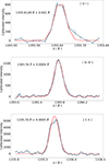 |
Fig. B.1. From top to bottom: O I 1355.6 Å, Si IV 1393 Å and C II 1336 Å average spectral profiles. The observed spectral lines (black curves) are averaged over the entire QS FoV taken on 12 November 2020. The best fit with a Gaussian is shown in red. Error bars on the black curves represent the standard deviation of the intensity at each wavelength point, computed across all spatial pixels in the QS FoV. Intensities are given in units of [erg cm−2 s−1 sr−1 Angstrom−1]. |
B.2. Error Calculation Procedure
The velocity measurements arise from the retrieved Gaussian fit parameters. In particular the parameter A1 representing the Gaussian center was used to derive the velocity. Thus, the total uncertainty for the velocity is estimated as follow:
 =
= +
+ +
+ +
+
where, the term σr accounts for the uncertainty in the reference wavelength and is equal to 0.13 km s−1. σc corresponds to the uncertainty from the O I wavelength calibration, with a value of 0.2 km s−1, σxy represents the median uncertainty in the measured wavelength, computed across all spatial pixels (i.e., both x and y image coordinates) and across the whole FoV of the three rasters, i.e., encompassing all the data acquired during the three IRIS scans. Finally, σf represents the offset between the FUVS and FUVL detectors.
All Tables
All Figures
|
Fig. 1. Overall view of AR12871. Panel A: Full-disk magnetogram clipped between ±500 G from HMI taken at 10:55 UT on November 10. The black box indicates the FoV shown in the following AIA 304 and 193 Å bands (panels B and C). Panel D: High-spatial resolution HiFI Hα image taken at 10:48 UT on November 10. Panel E: IRIS slit-reconstructed image in the center of the Mg II k3 line acquired between 11:03 UT and 11:52 UT on November 10. Panels F-G: HMI magnetogram clipped between ±500 G and continuum taken at 10:55 UT. The red box in the continuum image indicates the GRIS FoV. |
| In the text | |
|
Fig. 2. Restored Hα filtergrams acquired by HiFI instrument at GREGOR telescope showing fine structure of filament at various times on November 9 (top panels) and November 10 (bottom panels). The red and blue contours in the first panels indicate the positive and negative magnetic flux density obtained from SDO/HMI at level equal to ±200 G, respectively. The red box in the second-from-bottom panel represents the GRIS acquired scanned FoV from between 09:17:32 and 09:37:05 UT. Movies of the HiFI data showing the filament in the time interval between 08:44 UT and 11:02 UT (10:49 UT) on November 9 and 10 are available online. |
| In the text | |
|
Fig. 3. Top panel: Zoomed-in view of Hα filtergram for reference. Middle panel: GRIS slit-reconstructed He I line core intensity of the RoI acquired between 09:17:32 and 09:37:05 UT on November 10. Bottom panel: Stokes-I profiles, normalized to continuum intensity, observed at the red, blue, and orange (1, 2, and 3) positions shown in the He I line core map. Arrows point to thin, darker, elongated threads where the optical thickness of the He I line is higher than their own surroundings (Fig. 4). White contours represent a plasma velocity of about −1 km s−1. The shaded area indicates where the He I line core is calculated (see Sect. 3.2 for more details). The vertical lines represent the rest wavelengths for the three He I components as reported in Table 1 of Kuckein et al. (2012).
|
||
| In the text | |||
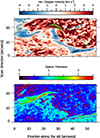 |
Fig. 4. He I Doppler velocity and optical thickness of GRIS observation, as calculated using the HAZEL code. Black and red contours represent plasma velocity of −1 km s−1. Green and yellow contours indicate plasma velocities greater than 10 and 15 km s−1. |
| In the text | |
|
Fig. 5. From top to bottom: Peak-intensity maps and spectral profiles in locations marked with an asterisk in the respective intensity maps and their relative fits of Mg II k, Si IV 1394 Å, and C II 1335 Å during the middle IRIS raster scan (11:03–11:52 UT). Original spectral line profiles are shown in black and corresponding Gaussian fits are shown in red (for Si IV and C II spectral lines). |
| In the text | |
|
Fig. 6. Peak-radiance maps Mg II (top), C II (middle), and Si IV (bottom). These maps result from the three IRIS rasters reported in Table 1. Contours in all middle panels indicate the high-resolution GRIS Hα filament contour. The red boxes represent the three panels shown in Fig. 8. |
| In the text | |
|
Fig. 7. Velocity maps for Mg II (top), C II (middle), and Si IV (bottom) observations. In all panels, black contour represents Mg II k3 intensity. |
| In the text | |
|
Fig. 8. Comparison of Hα and UV Mg II and Si IV IRIS intensity and Doppler velocity. From left to right: Hα intensity; Mg II k3 and Doppler velocity; Si IV peak intensity and Si IV Doppler-velocity maps for three RoIs (see the red boxes in the k3 intensity middle panels of Fig. 6). The Mg II k3 and Si IV Doppler-velocity maps are shown in the range from [−10, 10] to [−30,30] km s−1 as the original maps of Fig 10. In the Mg II k3 and Si IV intensity and Doppler-velocity maps, the red and blue contours represent upflows (−1 and −3 km s−1) and downflows (1 and 3 km s−1), respectively, corresponding to the Doppler velocities of Mg II k3 and Si IV. |
| In the text | |
|
Fig. 9. Mg II and Si IV intensity and velocity variation along slit drawn in third middle panel of Fig. 8. The shaded area indicates the width of the filament as seen in the Mg II intensity maps. Error bars in the Si IV velocity plot were retrieved as explained in Sect. 3.3. |
| In the text | |
|
Fig. 10. From top to bottom: Mg II peak difference (diff), peak asymmetry (asym), peak separation (sep), and Si IV FWHM maps. Red and black contours indicate Mg II k peak intensity in all panels. |
| In the text | |
|
Fig. 11. SDO/HMI magnetograms (top panels) and SDO/AIA 304 Å images at four representative times. The black boxes indicate the magnetic configuration of the AFS. Magnetograms are clipped ±500 G. Red and black arrows point new magnetic features described in the text. |
| In the text | |
|
Fig. B.1. From top to bottom: O I 1355.6 Å, Si IV 1393 Å and C II 1336 Å average spectral profiles. The observed spectral lines (black curves) are averaged over the entire QS FoV taken on 12 November 2020. The best fit with a Gaussian is shown in red. Error bars on the black curves represent the standard deviation of the intensity at each wavelength point, computed across all spatial pixels in the QS FoV. Intensities are given in units of [erg cm−2 s−1 sr−1 Angstrom−1]. |
| In the text | |
Current usage metrics show cumulative count of Article Views (full-text article views including HTML views, PDF and ePub downloads, according to the available data) and Abstracts Views on Vision4Press platform.
Data correspond to usage on the plateform after 2015. The current usage metrics is available 48-96 hours after online publication and is updated daily on week days.
Initial download of the metrics may take a while.