| Issue |
A&A
Volume 706, February 2026
|
|
|---|---|---|
| Article Number | A304 | |
| Number of page(s) | 22 | |
| Section | Extragalactic astronomy | |
| DOI | https://doi.org/10.1051/0004-6361/202554157 | |
| Published online | 18 February 2026 | |
Active galactic nucleus–host galaxy photometric decomposition using a fast, accurate, and precise deep learning approach
1
SRON Netherlands Institute for Space Research Landleven 12 9747 AD Groningen, The Netherlands
2
Kapteyn Astronomical Institute, University of Groningen Postbus 800 9700 AV Groningen, The Netherlands
3
Instituto de Radioastronomía y Astrofísica, Universidad Nacional Autónoma de México Apdo. Postal 72-3 58089 Morelia, Mexico
4
Leiden Observatory, Leiden University Einsteinweg 55 2333 CC Leiden, The Netherlands
★ Corresponding author: This email address is being protected from spambots. You need JavaScript enabled to view it.
Received:
17
February
2025
Accepted:
14
November
2025
Abstract
Aims. The identification of active galactic nuclei (AGNs) is extremely important for understanding galaxy evolution and its connection with the assembly of supermassive black holes (SMBHs). With the advent of deep- and high-angular-resolution imaging surveys such as those conducted with the James Webb Space Telescope (JWST), it is now possible to identify galaxies with a central point source out to the very early Universe. In this proof of concept study, we aim to develop a fast, accurate, and precise method of identifying galaxies that host AGNs and recover the intrinsic AGN contribution fraction (fAGN).
Methods. We trained a deep learning (DL) -based method, Zoobot, to estimate the fractional contribution of a central point source to the total light. Our training sample comprises realistic mock JWST images of simulated galaxies from the IllustrisTNG cosmological hydrodynamical simulations. We injected different amounts of the observed JWST point spread functions to represent galaxies with varying levels of AGN contributions. Galaxies in our training sample span a wide range of morphologies, including mergers. We analysed in detail the performance of our method as a function of various galaxy properties and compared it with results obtained from the traditional light profile fitting tool GALFIT. After training, we applied our method to real JWST observations in the COSMOS field.
Results. We find an excellent performance of our DL method in recovering the injected fAGN, in terms of precision and accuracy. The mean difference between the predicted and true fAGN is −0.002 and the overall root mean squared error (RMSE) is 0.013. The overall relative absolute error (RAE) is 0.076, and the outlier (defined as predictions with RAE > 20%) fraction is 6.5%. In comparison, using GALFIT, we achieve a mean difference of –0.02, a RMSE of 0.12, a RAE of 0.19, and an outlier fraction of 19%. We also investigate how these key performance metrics obtained from Zoobot and GALFIT vary as a function of the injected fAGN, redshift, signal-to-noise ratio, and galaxy size. In addition to the superior performance, our DL method has several other advantages over traditional methods. For example, it has a much higher success rate (even for highly disturbed or irregular galaxies) and is extremely fast. We applied our trained DL model to real JWST observations and found that 20% of the X-ray-selected AGNs and 8% of the MIR-selected AGNs are also identified as AGNs using a cut at fAGN > 0.2. When using fAGN > 0.1, these overlaps increase to 33% for the X-ray AGNs and 15% for the MIR AGNs. In summary, our DL-based method of identifying AGNs and estimating the AGN contribution fraction has a huge potential in future applications to large galaxy imaging surveys.
Key words: techniques: image processing / galaxies: active / galaxies: evolution
© The Authors 2026
 Open Access article, published by EDP Sciences, under the terms of the Creative Commons Attribution License (https://creativecommons.org/licenses/by/4.0), which permits unrestricted use, distribution, and reproduction in any medium, provided the original work is properly cited.
This article is published in open access under the Subscribe to Open model. This email address is being protected from spambots. You need JavaScript enabled to view it. to support open access publication.
1. Introduction
It is generally accepted that there exists co-evolution between supermassive black holes (SMBHs) and their host galaxies (Kormendy & Ho 2013). One manifestation of this co-evolution is the tight correlation between the mass of an SMBH and its host galaxy properties, such as the stellar velocity dispersion, bulge luminosity, and bulge mass (Gültekin et al. 2009; Beifiori et al. 2012; Graham & Scott 2013; McConnell & Ma 2013; Läsker et al. 2014). These correlations may hint at a fundamental connection between the central SMBH and the formation and evolution of its host galaxy. Theoretical models show that SMBH feedback, via radiative heating, outflows, or jets, could potentially explain these correlations, by regulating or halting the growth of itself and the host galaxy (e.g. Somerville et al. 2008; Booth & Schaye 2009; Weinberger et al. 2018; Davé et al. 2019). However, these correlations could also arise from merging events, in which mergers could explain, for example, the growth of SMBH mass and the stellar mass of the host galaxy (e.g. Croton 2006; Peng 2007; Hirschmann et al. 2010; Jahnke & Macciò 2011). To better understand the co-evolution (or not) of SMBHs and host galaxies, it is important to study their link at different cosmic times. At high redshifts, studies have to rely on accreting SMBHs, which are active galactic nuclei (AGNs), to be able to obtain SMBH mass estimates, and in particular Type I AGNs. It is also necessary to obtain quantitative measures of the physical properties of the host galaxies. However, the presence of a bright central AGN can make this task very difficult, particularly for the bulge component, as galaxies with significant contribution from the AGN to the total flux will appear to be more bulge-dominated (Pierce et al. 2010).
It is crucial to correctly separate the central AGN light from the host galaxy, across a wide range of galaxy types and redshifts. Good-quality optical imaging, with a high spatial resolution and signal-to-noise ratio (S/N), is needed to decompose the observed total light into contributions from the host galaxy and the central AGN. Traditionally, this is done in photometric data by fitting two-dimensional (2D) profiles to the galaxy’s light, using one (or more if needed) analytic profile to describe the galaxy (typically a Sérsic profile) and a point spread function (PSF) profile to describe the central point source. Many studies use GALFIT (Peng et al. 2002), one of the most widely used pieces of 2D surface brightness modelling software, to perform image-based decomposition of AGN and host galaxy light (e.g. Kim et al. 2008; Bentz et al. 2009; Gabor et al. 2009; Böhm et al. 2013; Schramm & Silverman 2013; Du et al. 2014; Urbano-Mayorgas et al. 2019; Son et al. 2022; Aird et al. 2022; Ji et al. 2022; Dewsnap et al. 2023; Zhuang & Ho 2023; Sturm & Reines 2024; Zhuang et al. 2024). However, there are some known technical issues with GALFIT. For example, in some cases, the minimisation algorithm used can be trapped in a local minimum, leading to unreliable fits. Other software has been used in an attempt to improve on GALFIT performance, such as PSFMC (Mechtley 2014), which is Markov chain Monte Carlo (MCMC) simultaneous fitting software, to perform multi-component profile fitting (Mechtley et al. 2016; Marshall et al. 2021), and LENSTRONOMY (Birrer et al. 2015; Birrer & Amara 2018), which uses particle swarm optimisation (Kennedy & Eberhart 1995) for χ2 minimisation, to reduce the likelihood of getting trapped in a local minimum when searching the parameter space, and MCMC for Bayesian parameter inference (Foreman-Mackey et al. 2013). The latter method was used by Li et al. (2021) to decompose a sample of X-ray-selected AGNs into quasars and host galaxy components, to investigate the properties of the host galaxies. However, these approaches all assume that the galaxy’s surface brightness profile can be well fitted by a single Sérsic profile (or combination of Sérsic profiles), which may not be the case, particularly for irregular galaxies, highly disturbed merging galaxies, or galaxies with complicated substructures.
Consequently, if Sérsic profiles cannot adequately describe the host galaxy light, they can introduce a systematic bias in the derived luminosity of the PSF component and of the host galaxy. In addition, if there is a significant contribution to the total flux from the central AGNs, it can lead to a bias in the morphology of the host galaxy, as it may appear to be more bulge-dominated (Pierce et al. 2010). Indeed, it is not always a good idea to represent a galaxy with a single Sérsic profile. Bentz et al. (2009) study AGN host galaxies at redshift z ≈ 0.7, by fitting their surface brightness distributions with a combination of Sérsic profiles (to account for the host galaxy’s light) and PSF profile (to describe the AGN component). They find that most galaxies in their sample are well described with two Sérsic profiles, in addition to the PSF profile, and a few of them required three or more Sérsic profiles to describe additional components such as bars. Another possible difficulty in decomposing the AGN from the host galaxy is the (sometimes significant) variation in the PSF in a given survey due to spatial and temporal changes or differences in galaxy spectral energy distributions (SEDs), as an incorrect PSF can bias the estimated contribution of the AGN to the total flux of the galaxy. Kim et al. (2008) performed 2D decomposition of Sérsic + PSF profiles to galaxies hosting AGNs in Hubble Space Telescope (HST) images and investigated the effect of realistic PSF mismatch, finding a systematic overestimation of the flux of the host galaxies, particularly for those containing bright AGNs.
Without additional information on the possible presence of AGN activity in a galaxy (e.g. from X-ray, MIR, or radio observations), it is not always easy to discern whether a galaxy has an AGN component in the form of a central point source from 2D surface brightness fitting, particularly for galaxies with very concentrated light profiles. This is because galaxy light in some cases could be more or less equally well described by a single Sérsic component or a combination of Sérsic + PSF profiles. A more complex model will always have a smaller χ2. Therefore, a better fit is not necessarily a good indicator to decide between different models. To mitigate this problem, Aird et al. (2022) fitted the HST imaging of a sample of galaxies in the Cosmic Assembly Near-infrared Deep Extragalactic Legacy Survey (CANDELS; Koekemoer et al. 2011; Grogin et al. 2011) at z = 0.5–3 with a Sérsic profile plus an additional central point source component and with a Sérsic profile only, and then used the residual flux fraction (RFF; Hoyos et al. 2011) to determine which was the best model. The RFF measures the fraction of the flux contained in the residual image that cannot be explained by fluctuations in the background. However, good estimates of the background and galaxy’s size are needed for this method.
In this work, we present a promising new methodology to determine the AGN contribution to the total flux of a galaxy in imaging data by combining deep learning (DL) methods and cosmological hydrodynamical simulations. Over the last decade or so, DL methods have been widely used for diverse astronomy applications (Dieleman et al. 2015; Huertas-Company et al. 2018; Walmsley et al. 2020; Margalef-Bentabol et al. 2020; Zanisi et al. 2021; Huertas-Company & Lanusse 2023). In particular, they show great success in different image-based astronomical problems, such as morphological classifications of galaxies (e.g. Huertas-Company et al. 2015; Domínguez Sánchez et al. 2018; Cheng et al. 2020; Walmsley et al. 2022a), merger identifications (Bottrell et al. 2019; Ferreira et al. 2020; Ćiprijanović et al. 2020; Pearson et al. 2022; Bickley et al. 2021; Margalef-Bentabol et al. 2024), and determining galaxies’ physical properties and structural parameters (Tuccillo et al. 2018; Simet et al. 2021; Euclid Collaboration: Bisigello et al. 2023). On the other hand, the use of cosmological hydrodynamical simulations allows us to create a comprehensive training sample of diverse and realistic galaxies, spanning a large range in redshift and mass.
Our DL model is trained on mock images of simulated galaxies with different levels of AGN contributions to the total flux. The construction of our training sample can easily incorporate the full information on the expected variations in the PSF. Therefore, our DL model can learn to infer the intrinsic AGN contribution fraction while automatically folding in the impact of different PSFs. In comparison, while it is possible to examine the goodness-of-fit for different PSF models for methods based on light profile fitting, such as GALFIT, in practice, it will be extremely time-consuming, particularly for large samples of galaxies. Another advantage of our DL-based method is that it does not rely on an assumed (and often simplified) galaxy surface brightness profile, which in many cases is not able to fully describe a galaxy’s light profile, and thus can introduce biases in the estimation of the AGN contribution. Finally, our method, like any other machine-learning-based method, has the advantage of being very fast to implement in new data once the DL model has been trained, making it much more computationally efficient than any traditional method based on light profile fitting.
This paper is organised as follows. In Sect. 2, we describe the observed James Webb Space Telescope (JWST; Gardner et al. 2006) imaging data used in this work and the generation of the corresponding mock JWST images of simulated galaxies selected from the IllustrisTNG. Of particular importance are the real JWST PSF models and their variations within the survey data. In addition, we introduce two AGN samples, selected in the X-ray and mid-infrared (MIR), which we use to compare with AGNs identified using our DL-based method. In Sect. 3, we first explain how we created the final images mimicking galaxies containing AGNs by injecting different levels of PSF contribution (taken as AGN contribution fractions) in the mock JWST images. Then we introduce our DL-based method (Zoobot; Walmsley et al. 2023) of recovering the intrinsic AGN contribution fraction in the observed total light. To compare with traditional light profile fitting-based methods, we also briefly describe GALFIT and how we use it in this work. In Sect. 4, we explore in detail the results from both methods and compare their performances as a function of various galaxy properties. We also present the first application of our DL-based method to real JWST data and compare with AGNs selected in the X-ray and MIR. Finally, in Sect. 5, we summarise the paper and highlight the main conclusions of our work.
Throughout the paper we assume a flat ΛCDM Universe with ΩM = 0.2865, ΩΛ = 0.7135, and H0 = 69.32 km s−1 Mpc−1 (Hinshaw et al. 2013). Unless otherwise stated, magnitudes are presented in the AB system.
2. Data
In this section, we first introduce the real JWST observations and the PSF models obtained from the COSMOS-Web survey. Then, we describe the synthetic JWST images generated using simulated galaxies selected from the IllustrisTNG cosmological hydrodynamical simulations. The observed and simulated datasets are combined later to create mock JWST galaxy images with different levels of AGN contribution.
2.1. JWST/COSMOS-WEB
COSMOS-Web (Casey et al. 2023, PIs: Kartaltepe & Casey, ID = 1727) is a 255-hour JWST treasury imaging survey observing the central area of the Cosmic Evolution Survey (COSMOS; Scoville et al. 2007) field, which is one of the most popular deep multi-wavelength survey fields. It covers a contiguous 0.54 deg2 region in four Near Infrared Camera (NIRCam) filters (F115W, F150W, F277W, and F444W), reaching a 5σ point source depth of 27.5 − 28.2 magnitudes. In parallel, a 0.19 deg2 area of Mid-Infrared Instrument (MIRI) imaging with the F770W filter is covered. For this work, we made use of the 0.28 deg2 JWST/NIRCam F150W images reduced by Zhuang et al. (2024). They used version 1.10.2 of the JWST1 pipeline with the Calibration Reference Data System (CRDS) version of 11.17.0., to reduce the uncalibrated NIRCam raw data retrieved from MAST2. The steps followed in the data reduction process are briefly summarised below:
-
Individual exposures of raw data were reduced using the Stage 1 pipeline Detector1Pipeline, in which they used some custom parameters to better flag large cosmic ray events and snowballs.
-
Fully calibrated individual exposures were obtained from running the Stage 2 pipeline Image2Pipeline, which performed wcs assignments, flat-fielding, and photometry calibration.
-
A 2D background was subtracted, after masking bad pixels and sources using SextractorBackground in the photutils package (Bradley et al. 2024).
-
Wisps (artefacts caused by scattered light in the mirror) and claws (features caused by scattered light coming from extremely bright stars) were subtracted.
-
Finally, single mosaics for each filter were produced using the Stage 3 Image3Pipeline by combining all calibrated images.
For each NIRCam mosaic, Zhuang et al. (2024) constructed three different PSF models. For this work, we used the global PSF models, which are produced using all of the point-like sources across the entire field of view (FoV) of each dither-combined mosaic. The median PSF full width at half maximum (FWHM) in the COSMOS-Web NIRCam mosaics is 61.1 mas for the F150W filter. The PSF in the NIRCam imaging has a fractional root mean squared (RMS) temporal variation in PSF FWHM of ∼2.4% for F150W, which is dominated by short-timescale fluctuation. In comparison, the spatial variation in PSF FWHM, dominated by random variations, is much larger, at a level of ≥5% for short-wavelength filters including F150W. For a full description of their data3 reduction method, we refer the reader to Sect. 2.1 of Zhuang et al. (2024). In Fig. 1, we illustrate the variations in the adopted global PSF models. We first stacked all 80 PSF models and then calculated the mean and the standard deviation pixel by pixel (displayed in the left and central panels of Fig. 1, respectively). The right panel of Fig. 1 shows the relative dispersion (or coefficient of variation), which is the standard deviation divided by the mean (pixel by pixel).
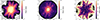 |
Fig. 1. Overview of the JWST/NIRCam F150W PSFs in COSMOS-Web. We stacked all available PSFs from Zhuang et al. (2024) and show the mean PSF (left), standard deviation (centre), and the coefficient of variation (right), calculated pixel by pixel. The PSFs have been re-binned to a pixel resolution of 0.03 ″/pixel, matching the resolution used for the synthetic image creation. The axes show the number of pixels, corresponding to 3″across. The colour bar shows the value of each pixel. |
We used the COSMOS2020 (Weaver et al. 2022) photometric catalogue to construct our sample of real JWST galaxies, within the COSMOS-Web area. For that, we used the Farmer’s version for the photometric catalogue. We used spectroscopic redshifts when available. Otherwise, we adopted the photometric redshifts (photo-z) listed in the COSMOS2020 catalogue, computed using the LePhare code (Arnouts et al. 2002; Ilbert et al. 2006). The photo-z precision, given by the normalised median absolute deviation (MAD), is around 0.01 × (1 + z) at i < 24.0 mag, and 0.03 × (1 + z) at 24.0 < i < 27.0 mag. Stellar masses (M*) were derived by La Marca et al. (2025), using the SED fitting tool CIGALE (Burgarella et al. 2005; Noll et al. 2009; Boquien et al. 2019), including AGN models. These stellar masses are consistent with the stellar masses presented in the COSMOS2020 photometric catalogue obtained by LePhare. We calculated the median bias, b, and the MAD between the two stellar mass estimates as follows:
 (1)
(1)
 (2)
(2)
where ΔM* = log10M*, LePhare − log10M*, CIGALE. We find b = −0.09 and MAD = 0.013. We constructed our galaxy sample in the redshift range 0.5 < z < 3, avoiding stars or areas affected by bright stars. Finally, we selected a stellar mass-complete sample by including galaxies with M* greater than either 109 M⊙ or the KS-based completeness limit from Weaver et al. (2022) for the COSMOS2020 catalogue:
 (3)
(3)
whichever is higher. The minimum stellar mass limit of 109 M⊙ was imposed to match the limit used for the simulated galaxy sample. In total, we included 25 596 galaxies in our stellar mass complete sample over the 0.28 deg2 analysed in this study.
2.2. AGN selections
We used the following two common AGN selection techniques to identify AGNs in our JWST sample and compared them with our DL-based methodology in Sect. 4.3,
-
X-ray AGN selection: For this selection, we used the X-ray photometry data from the Chandra COSMOS Legacy survey (Civano et al. 2016; Marchesi et al. 2016). From the catalogue of optical and infrared counterparts provided by Marchesi et al. (2016), we selectd sources with a final counterpart identification flag of 1 (secure) or 10 (ambiguous). We then cross-matched this catalogue using the optical coordinates with our selected sources in COSMOS2020. We selected secure X-ray AGNs requiring DET_ML (the maximum likelihood detection) > 10.8 in the hard or soft band. This selection yields a total of 223 X-ray AGNs within our final sample.
-
MIR AGN selection: For this selection, we used the Spitzer/MIPS 24 μm data, provided by the COSMOS-Spitzer programme (Sanders et al. 2007), and the MIR data from the four channels of the Spitzer/IRAC Cosmic Dawn Survey (Euclid Collaboration 2022). We followed Chang et al. (2017) to identify AGNs by their MIR emission. We limited the selection to those galaxies with Spitzer/MIPS 24 μm flux F24 μm > 20 μJy, which is the 1σ total noise (instrument and confusion noise). Additionally, we required S/N > 5 in each IRAC channel. Then, we applied the colour−colour criteria in Chang et al. (2017) to select AGNs:
 (4)
(4) (5)
(5) (6)
(6) (7)
(7)where x = m3.6 μm − m5.8 μm and y = m4.5 μm − m8 μm. Magnitudes are expressed as AB magnitude. Applying these criteria results in 680 MIR-selected AGNs in our final sample.
2.3. Mock JWST images
The IllustrisTNG project (Nelson et al. 2019; Pillepich et al. 2018; Springel et al. 2018; Nelson et al. 2018; Naiman et al. 2018; Marinacci et al. 2018) is a series of cosmological hydrodynamical simulations of galaxy formation and evolution, with three different runs that differ in volume and resolution. These runs are TNG50, TNG100, and TNG300, with comoving length sizes of 50, 100, and 300 Mpc h−1, respectively. The initial conditions for all runs are drawn from the Planck results (Planck Collaboration XIII 2016). For this work, we used TNG100 (better resolution than TNG300 but still with a big enough volume to contain a sufficiently large number of galaxies), which contains 18203 dark matter (DM) particles with a mass resolution of MDM, res = 7.5 × 10⁶ M⊙. In comparison, the baryonic particle resolution of TNG100 is Mbaryon res = 1.4 × 10⁶ M⊙. We refer the reader to Pillepich et al. (2018) for more details on IllustrisTNG.
In this work, we selected galaxies from 14 simulation snapshots (numbers 67, 64, 61, 58, 55, 52, 49, 46, 43, 40, 37, 33, 29, and 25), which correspond to redshifts from z = 0.5 out to 3. The time step between each snapshot is roughly ∼480 Myr over this redshift interval. We selected all galaxies from these snapshots with stellar mass M* > 109 M⊙ to ensure that most galaxies have a sufficient number of stellar particles (hence reasonably well resolved), with the lowest mass galaxies in TNG100 (M* = 109 M⊙) consisting of 714 particles. We randomly choose a total of ∼12 000 galaxies from this selection in mass and redshift to create our training sample. Every galaxy in IllustrisTNG has a complete merger history available from applying the SUBLINK algorithm on baryon-based structures (Rodriguez-Gomez et al. 2015). We used these merger trees to identify major mergers and non-merger galaxies. Specifically, major mergers are defined as galaxies with stellar mass ratios > 1:4 and that will either have a merger event in the following 0.8 Gyr (pre-mergers) or have had a merger event in the last 0.3 Gyr (post-mergers). Consequently, galaxies that do not satisfy these conditions are considered non-mergers.
For each galaxy, we generated a synthetic JWST/NIRCam F150W observation from the simulations with the following steps:
-
First, we created a smoothed 2D projected map (Rodriguez-Gomez et al. 2019; Martin et al. 2022). For each stellar particle in the simulation, we assigned an SED based on its mass, age, and metallicity, using the (Bruzual & Charlot 2003) stellar population synthesis models, with a Chabrier (2003) initial mass function. These SEDs were integrated through the JWST/NIRCam F150W filter transmission curve to obtain the flux contribution of each particle in that band. The spatial distribution of flux was smoothed using an adaptive kernel to create the 2D map. This approach does not include full radiative transfer calculations, and therefore dust attenuation and emission lines are not modelled. The images were produced with the same pixel resolution as the real JWST observations (0.03 ″/pixel), and have a physical size of 50 × 50 kpc.
-
Second, each image was convolved with a randomly chosen global JWST F150W PSF model (out of 80 in total, as derived by Zhuang et al. 2024). This step ensures that our training sample contains the full information on the (spatial and temporal) variation in the PSF.
-
Third, Poisson noise was added to each image to account for the statistical variation in a source’s photon emissions over time.
-
Lastly, each image was injected into cutouts of real JWST F150W sky cutouts. This step ensures that a fully realistic background and noise are included in our training data.
In the final step, we followed the same approach as in Margalef-Bentabol et al. (2024). To obtain cutouts of the real JWST sky, we first generated a catalogue of sources that we wanted to avoid within the central region of the cutouts. Starting from the ‘Farmer’ version of the COSMOS2020 catalogue (Weaver et al. 2022), we set the flag FLAG_COMBINED equal to 0 to select areas that are not affected by bright stars or large artefacts, as recommended by the COSMOS team. We then made use of the star-galaxy separation provided in the Le Phare photo-z, selecting sources with the star-galaxy flag lp_type equal to 0 (galaxy) or 2 (X-ray source). Finally, we restricted our selection only to z < 3 sources in the COSMOS-Web field. The final catalogue contains relatively bright sources, with average magnitudes being: HSC-i = 25.6 mag, UVISTA-H = 24.7 mag. Then, we generated random sky coordinates such that there are no catalogued bright sources within a circular radius of 6.5″. This radius corresponds to the estimated source density of the area from which we extracted the cutouts. These criteria ensure that there are no bright sources in the centre of the cutouts, where the synthetic galaxies will be injected, but still allow for faint background galaxies. The random coordinates were then used as the centres for the sky cutouts, in which to inject the simulated galaxies, after performing sanity checks to ensure that no artefacts, stellar spikes, or bad or saturated pixels were present.
To have a uniform dataset to train our DL model and to speed up computation, we cut all images to 128 × 128 pixels, without changing the pixel scale of 0.03″/pixel. In other words, the images are 3.84″across, corresponding to roughly 23–33 kpc in physical scale over the redshift range of our sample (i.e. 0.5 < z < 3).
3. Methods
In this section, we first described the construction of the mock JWST/NIRCam host galaxy images with different injected levels of AGN contribution. Then we introduce the two methods (our method based on DL and GALFIT based on 2D surface brightness fitting) used to estimate the AGN contribution fractions.
3.1. Mock AGN injection
To simulate images of galaxies with AGNs, we injected a central point source into the host galaxy image. The observed JWST PSF models as described in Sect. 2.1 were used as the central point source. In order to create different AGN contribution fractions, the relative brightness of the PSF was adjusted before injecting it into the mock JWST images described in Sect. 2.3.
The AGN contribution fractions were chosen to range from 0.0 to 0.95 in increments of 0.05, for a total of 20 different levels. For any given AGN contribution fraction, fAGN, the injected image was created as follows. First, the PSF image was transformed into a pixel scale of 0.03″/pix, the same as the simulated images. Then, the flux of the PSF image was measured within a 2″aperture using the aperturephotometry function of the photutils package (Bradley et al. 2024). This aperture size corresponds to sizes between 13 kpc and 18 kpc in our redshift range. The PSF image was normalised using this flux, so it could be easily adjusted later. The flux of the host galaxy image, Fhost, was measured in the same way. The AGN contribution fraction (i.e. contribution to the total light) is then defined as
 (8)
(8)
where FAGN is the flux of the AGN. Afterwards, the normalised PSF image was multiplied by FAGN, which can be derived from Eq. (8):
 (9)
(9)
Finally, the scaled PSF image was added to the host galaxy image.
For each galaxy, five different images were created with five different AGN contribution fractions, chosen randomly from the 20 possible discrete AGN contribution fractions. Example images of these simulated galaxies (from bright to faint) with varying levels of AGN contribution can be seen in Fig. 2. Visually, it is clear that it can be very difficult to discern the presence of the host galaxy when the AGN contribution fraction is large, particularly for fainter and higher-redshift objects. Later, we examined how well we can recover fAGN as a function of the intrinsic AGN contribution fraction, redshift, galaxy size, S/N, etc, using a set of common performance metrics.
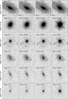 |
Fig. 2. Example mock JWST/NIRCam F150W images with varying levels of AGN contribution. The images have been generated to mimic JWST observations and include realistic JWST noise and background. Each row corresponds to a different galaxy, with no AGN contribution in the left panel and increasing AGN contributions in the rest of the panels. We show four example galaxies with different magnitudes, from the brightest (top) to the faintest (bottom). Images are 3.84″across and are displayed with an inverse arcsinh scaling. |
3.2. Deep learning CNN
Zoobot (Walmsley et al. 2023) is a Python package used to measure detailed morphologies of galaxies (such as spiral arms, bars, and bulges) using DL, based on the idea of successive layers of learned representations. Zoobot includes convolutional neural networks (CNNs, Fukushima 1988; LeCun et al. 2015) and vision transformer models (Dosovitskiy et al. 2021; Dehghani et al. 2023). These models are pre-trained on many millions of labelled galaxies, derived from the visual classifications of the Galaxy Zoo project (Lintott et al. 2008) on real images of galaxies selected from surveys such as the Sloan Digital Sky Survey (SDSS), Hyper Suprime-Cam (HSC), and Hubble (Willett et al. 2013, 2017; Simmons et al. 2017; Walmsley et al. 2022a,b). The models are designed to be easily adaptable to new tasks (classification or regression tasks) and galaxy surveys with a minimal amount of new labelled data.
Some of the available models in Zoobot belong to the family of ConvNeXts (Liu et al. 2022). They are pure convolutional models constructed by optimising the ResNet (He et al. 2015) architecture to bear resemblance with vision transformers (Vaswani et al. 2017; Liu et al. 2021), in which the design choices such as the use of the Gaussian error linear unit (GELU) activation function or inverted bottleneck CNN blocks (which are a specialised type of residual block more computationally efficient than normal residual blocks) are proven to improve the performance of a purely CNN model and can compete with transformer models in terms of accuracy and scalability.
For this work, we chose a ConvNeXt-Base architecture, which was pre-trained on the Galaxy Zoo dataset of over 820k images and 100 million volunteer votes on morphological questions. In order to perform a regression task (as is the case in this study), we added a linear head with a sigmoid function (to restrict the output to be between 0 and 1) and used a mean squared error loss function to train the network. A diagram of the ConvNeXt-Base network can be seen in Fig. 3. For this work, we retrained the last two blocks of the network and the linear head, while the rest of the network parameters were frozen to keep the optimal values found for the pre-trained data from Galaxy Zoo. Our model was trained on a V100 GPU and took 72 hours to complete. Once the model was trained, it took Zoobot 6 × 10⁻³ seconds to predict one galaxy.
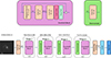 |
Fig. 3. Architecture of ConvNeXt-Base network (bottom) with a four-stage feature hierarchy, which allows us to extract features on different scales. On top of each stage, we show the dimension of the feature maps, with the width and height decreasing as the network deepens, while the filter size increases. The top left diagram shows the internal structure of ConvNeXt Block. The top right diagram shows the internal structure of Downsample. The LN and GELU represent a layer normalisation and a Gaussian error linear unit activation function, respectively. |
We split our sample of mock JWST images into training and test sets, with a 90/10 split. The distribution of the injected AGN contribution fraction in the training and test datasets can be seen in Fig. 4. The training dataset was used for training Zoobot. A validation set of 10% of the training data was used to monitor the performance during training. The test set was used to determine the performance of the final model on data that had never been seen before by the algorithms. To ensure the test set cannot be learned by simply interpolating from the training set, the galaxies were split into the train, validation, and test sets in a way that the five iterations of the same galaxy (with different injected AGN contribution fractions) were only used in one of the splits. Furthermore, we randomly selected a subset of 4800 galaxies from the test set on which to directly compare the results from the DL methodology and surface brightness fitting with GALFIT. This subset was constructed in a way that for each snapshot, we randomly selected 400 galaxies with a uniform distribution of fAGN.
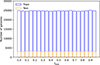 |
Fig. 4. Distributions of the injected AGN contribution fraction (as defined in Eq. (8)) in the training (blue) and test datasets (orange). The distributions are mostly uniform for both the training and test datasets. |
3.3. GALFIT
GALFIT (Peng et al. 2002) is a popular 2D fitting code used to model the surface brightness of an object with pre-defined analytic functions. GALFIT allows the user to fit any number of components and different light profiles (e.g. Sérsic, exponential disc, PSF, etc.). The best-fit model is obtained by χ2-minimisation using a Levenberg-Marquardt algorithm. A Sérsic profile generally describes well the light distribution of spheroidal or disc galaxies (even though it will not be able to represent highly disturbed or irregular galaxies). It has the following functional form,
![Mathematical equation: $$ \begin{aligned} \sum (R) = {\sum }_e exp \left\{ -\kappa _n \left[ \left( \frac{R}{R_e} \right)^{1/n} -1 \right] \right\} , \end{aligned} $$](/articles/aa/full_html/2026/02/aa54157-25/aa54157-25-eq10.gif) (10)
(10)
where Re is the effective radius, such that half of the total flux is contained within Re, ∑e is the surface brightness at Re, n is the Sérsic index (it determines the shape of the light profile, and n = 1 represents a disc, while n = 4 represents a spheroid), κn is a positive parameter that depends on n. On the other hand, the PSF profile can be used to describe a central point source such as the AGN. We can fit the surface brightness of each galaxy with a combination of Sérsic and PSF profiles in order to derive the contribution from a possible AGN component at the centre of the galaxy.
We ran GALFIT on the subset of 4800 galaxies from the test set. We first ran Sextractor (Bertin & Arnouts 1996) on all the test images to determine the central positions in pixels, x and y, the total magnitude of the galaxy, axis ratio (q), and effective radius (Re). Sextractor also produces a segmentation map in which all galaxies are identified and can be used to either mask neighbouring galaxies or fit them simultaneously with the central galaxy. In order to perform χ2-minimisation, GALFIT requires a sigma map. This sigma map was constructed by adding the Poisson noise contribution from the simulated galaxy (after injecting the AGN contribution) to the error map provided by the JWST data.
We ran GALFIT with a combination of a single Sérsic profile and a PSF model for the main central galaxy in each image. Neighbouring galaxies were masked, unless their light overlaps with the central galaxy, in which case they were fitted simultaneously with a Sérsic profile. The initial estimates of the model parameters can have an impact on whether GALFIT finds a good fit or not. That is why we ran GALFIT with different initial parameters of Sérsic index and magnitudes. We chose the best model to be the one with the lowest reduced χ2. For the Sérsic index of the main galaxy, we chose as initial values n = 1, 2, 4, alternatively. For the magnitudes of the Sérsic and PSF models, we used three different combinations of the initial parameters. In the first scenario, both models were set to be equal to a magnitude that corresponds to half of the total flux obtained from Sextractor. In the other two scenarios, the magnitude of the PSF (Sérsic) model was set to be 80% of the total flux, while the magnitude of the Sérsic (PSF) model was set to be 20%. For the rest of the parameters (position x and y, axis ratio, position angle, and effective radius), we used as initial values those obtained by Sextractor. In total, this resulted in nine different model configurations (three Sérsic index values × three magnitude combinations), from which we selected the one with the lowest reduced χ2 as the final best fit. For the neighbouring galaxies that were fitted simultaneously, we also used the Sextractor parameters plus a Sérsic index of n = 2. On average, GALFIT took 15 seconds per galaxy to complete the fitting procedure (2500 times slower than the prediction time from Zoobot), which resulted in a total of 90 hours to fill all nine model configurations (resulting from the different combinations of initial Sérsic indices and magnitudes) for the 4800 galaxies in our test subset.
In some cases, GALFIT did not converge and did not produce a fit at all. In other cases, even if GALFIT produced an output, it was clearly not a good fit for the surface brightness light. We only selected galaxies for which GALFIT produced a good fit; that is, for which there is a reduced χ2 < 5 and for which there are no non-physical parameters (for example, an effective radius smaller than 0.5 pixels or larger than the size of the image stamp, q < 0.1, and n < 0.5 or n > 10). In Fig. 5, we present good GALFIT fits of example galaxies containing varying amounts of injected AGN contribution fractions (from insignificant to dominant AGN contributions), with the original image, the model image (Sérsic + PSF), and the residual image (original - model) shown in different columns. After the best fit had been found, we created images of each model separately (Sérsic and PSF) using the parameters from the best fit. We then calculated the flux within an aperture of 2″in the Sérsic model, the PSF model, and the original galaxy image.
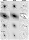 |
Fig. 5. Sérsic + PSF decomposition of four example galaxies (with AGN contribution fraction varying from high to low from top to bottom) on which we performed GALFIT. Images of the original galaxy, the model (Sérsic + PSF), and the residual (original−model) are shown from left to right. Images are 3.84″across and are displayed with an inverse arcsinh scaling. |
Finally, we calculated the AGN contribution fraction derived from running GALFIT in two slightly different ways. In the first method, we set the derived AGN contribution fraction to be equal to the ratio of the aperture flux from the PSF component to the aperture flux of the original galaxy image (which corresponds to the total flux of the galaxy within a 2″aperture). In the second method, we used as total flux (within a 2″aperture) the sum of the aperture fluxes of the PSF and the Sérsic model. We adopted these two different approaches to calculating the total flux of the galaxy in order to understand if there is any systematic bias in the Sérsic model, which could also impact the flux of the PSF model.
4. Results
In this section, we first present results from our DL-based method Zoobot. We analyse in detail how key performance metrics such as the root mean squared error (RMSE), relative absolute error (RAE), and outlier fraction vary as a function of the injected AGN contribution fraction, redshift, S/N, and galaxy size. Then, we compare these results with the performance obtained from running GALFIT on the same test set. Finally, we apply our DL-based method to the real JWST images of the stellar mass complete galaxy sample and compare AGNs identified using our method with AGNs selected in the X-ray and MIR.
4.1. Zoobot model performance
Here, we analyse the performance of the Zoobot model on the subset of 4800 galaxies from the test set. We first calculated the RMSE,
![Mathematical equation: $$ \begin{aligned} \mathrm{RMSE} = \sqrt{\frac{1}{n}\Sigma ^{n}_{i = 1} (f^i_{\rm AGN} [\mathrm{injected}] - f^i_{\rm AGN} [\mathrm{predicted}])^2}, \end{aligned} $$](/articles/aa/full_html/2026/02/aa54157-25/aa54157-25-eq11.gif) (11)
(11)
which measures the average difference between the predicted values from a model (e.g. Zoobot or GALFIT) and the actual injected values. In Fig. 6, we show the predicted values of fAGN, obtained from Zoobot, versus the real fAGN for all redshifts, which shows a very tight correlation across the whole dynamic range. Quantitatively, we found an overall value of RMSE = 0.013 for the Zoobot model, demonstrating very good recovery (in terms of both accuracy and precision) of the injected real AGN contribution fractions. In addition, the top panel of Fig. 6 shows the mean and the dispersion of the difference between the real and predicted values (ΔfAGN = fAGN [injected] −fAGN [Zoobot]) as a function of the injected AGN contribution fraction, with a value for the mean of ⟨ΔfAGN⟩= − 0.0018, and dispersion of σ(ΔfAGN) = 0.013. This shows that there is very little bias from the Zoobot predictions to the actual values, and it is independent of fAGN, as the difference between the real and predicted value over the whole range of fAGN is always below –0.0043. To check if the performance depends on galaxy structural properties, we further explore whether the Sérsic index impacts how well Zoobot can predict the AGN contribution fraction (see Fig. A.1) and find that for galaxies with n < 1 the RMSE increases by 30% (compared to the overall RMSE of 0.013), to RMSE = 0.017 and that high Sérsic indexes (n > 6) do not lead to worse predictions (i.e. similar RMSE to the overall RMSE of 0.013).
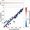 |
Fig. 6. Comparison between the real injected AGN contribution fraction and the AGN contribution fraction obtained from the Zoobot model on the subset of 4800 galaxies across the whole redshift range (0.5 < z < 3). The comparison shows a mean difference between the two quantities (ΔfAGN = fAGN [Injected] −fAGN [Zoobot]) of −0.0018 and an overall RMSE = 0.013. The solid diagonal line is the 1:1 line. The top plot shows the mean difference and its dispersion as a function of the injected AGN contribution fraction. The colour bar indicates the number of sources in each bin. |
In Fig. 7, we show the RMSE of the Zoobot predictions (purple lines) as a function of the injected AGN contribution fraction, redshift, S/N, and kron radius (rkron, calculated with SExtractor in the F150W filter). The solid lines show the RMSE of the whole test subset. To separately investigate how the performance might change for highly disturbed or irregular galaxies, we also show galaxies classified as mergers (dashed lines) and galaxies classified as non-mergers (dotted lines), separately. In general, the RMSE is slightly lower for non-merging galaxies, but the difference with mergers is very small. The RMSE is larger for lower values of the injected AGN contribution fraction and reaches a maximum mean value of 0.020. At fAGN > 0.2, Zoobot achieves smaller errors than the coefficient of variation in the PSF; that is, a smaller error than the error on the PSF resulting from the intrinsic temporal and spatial variations (shaded region of Fig. 7). In other words, the precision of our DL-based method is better than the intrinsic variations in the observed PSF. This is only possible because the DL method is trained on data that includes the full range of observed PSFs.
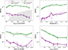 |
Fig. 7. RMSE as a function of the injected AGN contribution fraction (top left), redshift (top right), S/N (bottom left), and rkron (bottom right). The purple lines correspond to the results from Zoobot, and the green lines from GALFIT. The solid lines correspond to the whole sample, while the dashed and dotted lines correspond to the mergers and non-merger galaxies, respectively. The error bars show the 95% interval from bootstrapping the RMSE value. The performance of Zoobot is around a factor of ten better than GALFIT. The shaded region in the top left panel represents the fractional variation (standard deviation divided by the mean) of the PSF, considering the spatial and temporal variations. |
There is an increase in the RMSE with increasing redshift, with a maximum value of RMSE = 0.026 at z = 3, possibly because galaxies at higher redshifts are smaller and tend to have lower S/N (i.e. more dominated by noise). Indeed, we see that generally the RMSE increases with decreasing rkron and S/N. However, we also observe a small rise in RMSE at the highest S/N end, which is likely due to low number statistics in that bin; in such cases, even a single outlier can have a disproportionately large effect on the RMSE.
In Fig. 8, we show the RAE, which is the ratio between the absolute error divided by the real value4,
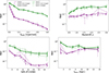 |
Fig. 8. Average RAE in bins of injected fAGN (top left), redshift (top right), S/N (bottom left), and rkron (bottom right), from the Zoobot predictions. The error bars correspond to the standard deviation of the data points in each bin. The purple lines correspond to the results from Zoobot, and the green, from GALFIT. The solid lines correspond to the whole sample, while the dashed and dotted lines correspond to the merger and non-merger galaxies, respectively. |
![Mathematical equation: $$ \begin{aligned} \mathrm{RAE} = \frac{|f_{\rm AGN}[\mathrm{injected}] - f_{\rm AGN} [\mathrm{predicted}] |}{f_{\rm AGN} [\mathrm{injected}]}. \end{aligned} $$](/articles/aa/full_html/2026/02/aa54157-25/aa54157-25-eq12.gif) (12)
(12)
The purple lines (solid lines represent the whole test subset, dashed lines mergers, and dotted lines non-mergers) show the relative error from the Zoobot predictions as a function of the injected AGN contribution fraction, redshift, S/N, and rkron (calculated by SExtractor in the F150W filter). We find that the relative error increases as fAGN decreases, particularly for fAGN < 0.1. While the RMSE only quantifies the absolute difference between real and predicted, the relative error does so in relation to the actual value. The relative error does not change much with redshift. But, similarly to the RMSE, it increases with decreasing S/N and decreasing rkron, as expected. Overall, there is a small difference between mergers (dashed lines) and non-mergers (dotted lines), with non-mergers having slightly higher relative errors in some cases.
Finally, we explore the outlier fraction in the Zoobot predictions. Here we define outliers as the Zoobot predicted AGN contribution fractions with an RAE of more than 20%; that is,
![Mathematical equation: $$ \begin{aligned} \frac{|f_{\rm AGN}[\mathrm{predicted}] - f_{\rm AGN}[\mathrm{injected}]|}{f_{\rm AGN}[\mathrm{injected}]}>20\%. \end{aligned} $$](/articles/aa/full_html/2026/02/aa54157-25/aa54157-25-eq13.gif) (13)
(13)
In Fig. 9, we show the outlier fraction as a function of the injected AGN contribution fraction, redshift, S/N, and rkron in purple lines. The overall outlier fraction for the whole sample is 6.5%. At intermediate to high levels of AGN contribution, the outlier fraction is extremely low (close to zero). However, at low levels of injected AGN contribution fractions, particularly for fAGN < 0.1, it increases very sharply with decreasing fAGN. This behaviour is partly caused by our definition of outliers (i.e. it depends on whether we use a threshold on relative or absolute errors). The outlier fraction remains more or less constant as a function of redshift and galaxy size. Concerning the S/N, there is only a small increase in the outlier fraction for S/N < 3. At S/N > 3, the outlier fraction drops to almost zero. There is no significant difference in the outlier fractions between mergers (dashed lines) and non-mergers (dotted lines). In Table 1 we summarise the results obtained from Zoobot, in terms of the RMSE, RAE, mean difference, and outlier fractions (at different percentage levels, 20% and 30%) for the whole test sample and for mergers and non-mergers separately.
Performance statistics for Zoobot and GALFIT.
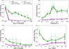 |
Fig. 9. Outlier fraction (calculated as the fraction of galaxies with RAE > 20%) as a function of the injected AGN contribution fraction (top left), redshift (top right), S/N (bottom left), and rkron (bottom right). The purple lines correspond to the results from Zoobot, and the green, from GALFIT. The solid lines correspond to the whole sample, while the dashed and dotted lines correspond to the merger and non-merger galaxies, respectively. |
4.2. GALFIT performance
We now analyse the results of the derived AGN contribution fraction after performing 2D light profile fitting on the same subset as Sect. 4.1. Each galaxy was fitted with a single Sérsic and a PSF component, which describe the host galaxy and central source component, respectively. The AGN contribution fraction derived from this method was calculated by dividing the flux (within a circular 2″aperture) of the PSF model by the total flux of the galaxy (within the same aperture). As mentioned before, we can calculate the total flux in two ways: the first one is calculated from the original galaxy image (FGalaxy) and the second one from the total model of the galaxy (FSérsic + FPSF). We compare the two slightly different AGN contribution fractions derived using GALFIT to better understand any possible bias introduced by fitting a Sérsic model.
In Fig. 10, we compare the AGN contribution fraction obtained from running GALFIT (in the two ways explained above) with the real injected AGN contribution fraction. When we calculate the AGN contribution fraction by dividing by the total flux of the galaxy, we find that RMSE = 0.12, with a mean difference (between predicted and real value) of ⟨ΔfAGN⟩= − 0.018 and dispersion: σ(ΔfAGN) = 0.12. However, when we consider the AGN contribution fraction calculated completely from the model, we obtain slightly worse results, with RMSE = 0.17, ⟨ΔfAGN⟩= − 0.075 and σ(ΔfAGN) = 0.15. This highlights how an inaccurate Sérsic model can bias the recovered AGN contribution fraction. From now on, we only show the results from calculating the total flux of the galaxy from the original galaxy image. The RMSE obtained from GALFIT is more than ten times higher than that obtained from Zoobot. There seems to be a small systematic offset (as seen by the mean difference) that is not found in the Zoobot results, and a larger spread between predicted and real (injected) AGN contribution fractions than from Zoobot. In terms of dependence on galaxy structural properties, we find that galaxies with n < 1, have an increased RMSE of 34%, and it is even higher when the injected AGN contribution fraction is small (fAGN < 0.2), which means that GALFIT results are more affected by low Sérsic index than our DL methods. We do not see a worse prediction of the fAGN for galaxies with high Sérsic index for either method (see Fig. A.2 for more details on the effect of Sérsic index in predicting fAGN).
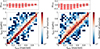 |
Fig. 10. Comparison between the real injected AGN contribution fraction and the AGN contribution fraction obtained from GALFIT fitting, obtained by dividing the PSF flux by the total flux. Left: Total flux corresponds to the flux measured within a 2″aperture in the original image. Right: Flux measured within a 2″aperture in the model (Sérsic+PSF). In both cases, the PSF flux was measured within the same aperture in the model PSF image. The dispersion in the left panel corresponds to RMSE = 0.12, and in the right, RMSE = 0.17. The colour bar provides the number of sources in each 2D bin. |
Figures 7, 8, and 9 show the RMSE, relative error, and outlier fractions, respectively, as defined in the previous section. The green lines show the results from the AGN contribution fraction obtained from the GALFIT fitting. We see similar trends to those from Zoobot, but with larger values (indicating significantly worse performance). We see that, over all the galaxy properties (fAGN, redshift, S/N, and rkron) considered, the RMSE is always higher for GALFIT than for Zoobot. Similar to the Zoobot results, we observe a small increase in RMSE with increasing redshift and with decreasing S/N. We also observe a general decrease in the RMSE with increased AGN contribution fractions, although the RMSE also decreases at fAGN < 0.1. This decrease for very low AGN contribution fractions seems to arise due to the real AGN contribution fraction value being very small. Actually, when looking at how the RAE changes with AGN contribution fraction (Fig. 8), we see that it increases significantly as fAGN decreases. The same results are observed with Zoobot, but again, the total RAE for GALFIT is higher than for Zoobot, independently of fAGN, redshift, S/N or rkron. Consequently, the outlier fraction is also always higher for GALFIT, with a dramatic increase, which was also observed in the previous section, at fAGN < 0.2. In Table 1, we summarise the results on the performance metrics obtained from GALFIT, for the two ways to calculate the AGN contribution fractions – that is, by determining the total flux of the galaxy (within 2″) from either the original galaxy or the GALFIT model (Sérsic+PSF) – and show the RMSE, RAE, and outlier fractions (at different percentage levels, 20% and 30%) for the whole test sample.
We find that 24 ± 1% of all the galaxies from the sub-sample test set have no fit from GALFIT or a bad one. However, there is no significant difference in the fraction of mergers and non-mergers that have a bad or no fit. In Fig. 11, we show that GALFIT fails more often for galaxies with high or low AGN contribution fractions (particularly at fAGN ≳ 0.8 and fAGN ≲ 0.2), higher redshift, lower S/N and very small galaxies. Therefore, even though we have previously seen that both the RMSE and RAE are relatively low at fAGN ≳ 0.8, GALFIT fails to find a good fit in that regime for 46 ± 3% of the galaxies, while at fAGN ≲ 0.2 GALFIT fails for 25 ± 2% of galaxies. GALFIT also fails more often at the higher redshifts (28 ± 1% of fails for z > 1), compared to 19 ± 1% for the rest of the sample, and 14 ± 2% in the lowest redshift bin. Finally, GALFIT is more likely to fail for faint galaxies (with low S/N) and for very bright ones (with high S/N). There are 75 ± 3% of galaxies with no good fit for S/N > 8 and 24 ± 4% for S/N < 3. These results highlight the importance of good-quality imaging in order to find a good fit to the galaxy’s light with GALFIT, while our DL-based method can always determine a galaxy’s AGN contribution fraction with good accuracy and precision regardless of these galaxy properties (within the dynamic ranges tested in this work).
 |
Fig. 11. Number of galaxies for which GALFIT returns a good fit (blue histograms) and for which there is a bad fit or no fit from GALFIT (red histograms), as a function of the injected AGN contribution fraction (top left), redshift (top right), S/N (bottom left), and rkron (bottom right). GALFIT tends to fail for bright galaxies, galaxies with low S/N, or with very high or low injected AGN contribution fractions. |
4.3. Application to JWST galaxies
Finally, we applied the trained DL model to our stellar mass complete sample of real JWST galaxies as described in Sect. 2.1. In Fig. 12, we show the distribution of the DL predicted AGN contribution fractions. Considering the overall RMSE of our DL-based method in recovering the intrinsic fAGN is 0.013, a 5σ cut corresponding to fAGN = 0.065 can be used to select galaxies for which the method is confident in identifying a non-negligible contribution from a central point source component. Indeed, the distribution shown in Fig.12 clearly separates at around this 5σ cut value.
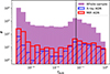 |
Fig. 12. Distribution of the predicted fAGN on the sample of JWST galaxies (purple). The blue and red histograms show the predictions for the X-ray and MIR AGNs within our sample, respectively. The black line (fAGN = 0.065) represents the 5σ value with respect to the overall mean RMSE. The x and y axes are displayed on a logarithmic scale. |
It is important to note, however, that the AGN contribution fraction measures the nuclear light excess and may not necessarily be interpreted as exclusively tracing AGN emission, since compact star-forming regions, stellar clusters, or other unresolved components, particularly at high redshift, could also partially contribute to the detected central point-source signal. Additional multi-wavelength and/or spectroscopic diagnostics are therefore needed to confirm or refute the AGN nature of these candidates.
Many traditional methods of selecting AGNs use a binary approach to separate galaxies into those that host AGNs and those that do not. In reality, there is a continuous distribution of the AGN contribution fraction. Therefore, although a binary AGN versus non-AGN selection approach is useful in identifying galaxies with dominant AGN, it is limited in the sense that it does not reflect the full spectrum. Adopting the 5σ cut at fAGN = 0.065, we find a total of  galaxies hosting a non-negligible level of AGN activity in the 0.28 deg2 of the COSMOS field analysed in this paper. The uncertainties correspond to varying the threshold by the RMSE of our method (0.013), i.e. counting galaxies with fAGN > 0.065 ± 0.013, which yields lower and upper thresholds of 0.052 and 0.078, respectively. Therefore, with respect to the total size of our stellar mass complete sample, 13% of the galaxies are identified by our method to have a non-negligible level of AGN contribution in the JWST/NIRCam F150W filter.
Using the continuous parameter, fAGN, predicted by our DL method, users can choose different cuts on AGN contribution fraction to construct an AGN sample depending on the specific requirements. For example, we can classify galaxies as AGNs based on the fractional AGN contribution, using a cut at fAGN > 0.2, which leads to  galaxies being classified as AGNs over 0.28 deg2. With a less conservative cut at fAGN > 0.1, we find
  AGNs within our sample. Furthermore, we find that there are 18 galaxies with fAGN > 0.7 (shown in Fig. B.1). There are five galaxies with spectroscopic information within those 18 galaxies. Four out of those five (i.e. 80%) show optical broad lines in their spectra, as indicated by the specific flag in the release catalogue of spectroscopic redshifts available to the COSMOS collaboration from KECK follow-up observations (Khostovan et al., in prep.). Based on this, we conclude that most galaxies with high fAGN, as predicted by our method, are consistent with optical spectroscopically confirmed AGNs (when that information is available).
To further investigate the nature of our fAGN-selected galaxies, we performed a complementary analysis, which is presented in Appendix C. Because the JWST/NIRCam F150W filter probes different rest-frame wavelengths across our redshift range, we train additional networks using the other three NIRCam filters available in COSMOS-Web (F115W, F277W, and F444W) to partially mitigate redshift effect and provide additional colour information. In Appendix C.3 we examine the colours of AGN and non-AGN galaxies, as well as MIR-selected AGNs. We find that our fAGN-selected sources display systematically redder colours than non-AGNs, in the same direction as the traditionally selected MIR AGNs, which may be consistent with emission from dust heated by AGNs.
Next, we compare our AGNs based on the estimated fAGN with AGN samples selected via X-ray detection or MIR colours. Using the cut at fAGN > 0.2, we find that 20% of the X-ray AGNs are also selected as AGNs based on the estimated fAGN, while 8% of the MIR-selected AGNs are also selected by our method. If we use a less conservative cut at fAGN > 0.1, then the overlapping fractions increase for both AGN selections, to 15% overlap with the MIR-selected AGNs and 33% overlap with the X-ray AGNs. There is, however, a large fraction of X-ray and MIR AGNs with a very low AGN contribution fraction, fAGN < 0.1, and therefore these were not selected as AGNs by our DL method based on a 0.1 threshold on fAGN. This is to be expected, as it is well known that some X-ray and MIR AGNs are not detected by optical diagnostics (Satyapal et al. 2008; Smith et al. 2014; LaMassa et al. 2019; Comerford et al. 2022). This phenomenon could be explained by a bright host galaxy that dilutes the light of the AGN or by the presence of copious dust in the host galaxy, particularly when the galaxy is viewed edge-on, causing heavy obscuration (Satyapal et al. 2008; Jackson et al. 2012; Smith et al. 2014; Hickox & Alexander 2018; Fitriana & Murayama 2022). In Figs. B.2 and B.3 we show a random subset of the X-ray and MIR AGNs with fAGN < 0.065 (i.e. below the 5σ cut based on the overall RMSE of our DL method), respectively. Many of these galaxies display spiral, clumpy or edge-on morphologies, in which higher dust content is expected. And in all cases, they do not show any obvious nuclear component in the JWST/NIRCam F150W images, which explains the low predicted fAGN despite being classified as X-ray or MIR AGNs. A similar analysis using the same methodology was done on Euclid/VIS imaging (Euclid Collaboration: Margalef-Bentabol et al. 2026), where the overlaps with X-ray and MIR AGN selections were found to be higher. However, such variations are expected, as the resulting overlap fractions depend sensitively on several factors, including the intrinsic luminosity of the AGN population, the rest-frame wavelength range probed by each dataset, and the specific selection criteria.
We also computed the fraction of our AGNs, based on fAGN, that are found in the X-ray and MIR-selected AGN samples. For sources with fAGN > 0.2, we find that 6% are also X-ray AGNs and 5% are MIR AGNs. These fractions decrease to 4% and 3%, respectively, when considering a lower threshold of fAGN > 0.1. This trend suggests that X-ray and MIR selection methods preferentially identify more powerful AGNs, while our optical method is sensitive to a broader population, including less dominant or possibly obscured AGNs. This result reinforces the notion that different AGN selection techniques probe different AGN populations. We also note that an fAGN value above the selection threshold does not necessarily indicate true AGN activity; in some cases, the fAGN signal may arise from central sources unrelated to AGNs. We also investigate whether the fAGN distributions differ for galaxies identified as X-ray or MIR AGNs. As shown in Fig. 12, the distributions for these sub-samples closely follow that of the whole sample, indicating that our method predicts similar fAGN values regardless of whether the galaxy is independently classified as an AGN in X-ray or MIR. This suggests that the low overlap is not due to a bias in how our method treats X-ray or MIR AGNs, but rather reflects the differences in the AGN populations each method is sensitive to.
In Fig. 13, we show the normalised distributions of the predicted fAGN in the different AGN samples. The X-ray-selected AGNs tend to dominate at higher AGN contribution fractions fAGN > 0.1, indicating better correspondence with optically dominant AGNs. For comparison, we also plot the distribution of the predicted fAGN in the ‘non-AGN’ sample, which corresponds to galaxies not identified as X-ray or MIR AGNs in our sample. We can see that while a large fraction (around 90%) of the non-AGNs have fAGN < 0.1, a small fraction (around 4%) of them do have predicted fAGN > 0.2, indicating that they can be AGNs missed by the X-ray and MIR selections. In fact, it is widely known that the X-ray-selected AGNs can miss a significant fraction of AGNs with strong optical emission lines, particularly those that are heavily absorbed (Heckman et al. 2005), while the MIR selection can miss low-luminosity AGNs or AGNs in host galaxies dominated by starburst, or radio-loud AGNs (Hainline et al. 2016; Truebenbach & Darling 2017). Out of the 18 galaxies with fAGN > 0.7 from our DL-based method as discussed previously, only a third of them are identified as MIR or X-ray AGNs. However, we expect that most of those 18 galaxies would be optically dominant AGNs, based on the fact that five out of the 18 galaxies were followed up in optical spectroscopy, and four exhibit broad lines in their spectra.
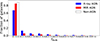 |
Fig. 13. Fraction of galaxies in bins of predicted AGN contribution fraction in the X-ray AGNs, MIR AGNs, and ’non-AGNs’ samples. |
The top panel of Fig. 14 shows the overlapping fraction of AGNs also identified using our DL method based on the predicted AGN contribution fraction as a function of the adopted cut on the X-ray luminosity, LX, or the rest-frame 6 μm luminosity, L6 μm, for the X-ray- and MIR-selected AGNs, respectively. We see that the overlapping fraction of AGNs also selected by our model increases with increasing luminosity (more slowly for the MIR AGNs). This is expected as the X-ray luminosity and the rest-frame 6 μm luminosity (which are indicators of the power of the X-ray or MIR-selected AGNs) correlate, albeit with significant scatter, with the luminosity of the AGN component in the JWST/NIRCam F150W filter, LAGN (calculated as the total luminosity in that filter multiplied by fAGN). We show these correlations in the bottom panel of Fig. 14, only for galaxies with fAGN > 0.065 for which we can confidently identify a central point source contribution. The strongest correlation is found for the X-ray AGNs detected in the soft band, and the weakest correlation is found in the MIR AGNs.
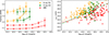 |
Fig. 14. Top: Overlapping fraction of AGNs also identified by our DL method as a function of the adopted cut on the X-ray or the rest-frame 6 μm luminosity for the X-ray and MIR-selected AGNs. The solid lines show the overlapping fraction by applying a cut at fAGN > 0.2, while the dashed lines show the overlapping fraction if we select AGNs by requiring fAGN > 0.1. Bottom: AGN luminosity in the JWST/NIRCam F150W filter versus the X-ray luminosity or the rest-frame 6 μm luminosity, for the X-ray-selected or MIR-selected AGNs. The dash-dotted lines show the respective linear fits. |
5. Summary and conclusions
In this paper we have presented a new DL-based method, Zoobot, of determining the AGN contribution fraction to the total flux of a galaxy, trained on realistic mock images generated from cosmological hydrodynamical simulations. Specifically, we constructed the training sample for our DL model from the IllustrisTNG simulations. First, we mimicked the observational effects of the JWST/COSMOS-WEB survey in the NIRCam F150W filter by using the same pixel scale, convolving with the full range of the survey PSFs, adding Poisson noise, and finally adding the real JWST sky background. Then, we artificially added an AGN component (approximated by the PSF) at different levels to represent different AGN contribution fractions to the total flux. After training our model, we analysed the performance results in detail on a test sample. Furthermore, we used GALFIT to fit the 2D light profile of the galaxies in the test sample with a combination of Sérsic + PSF profiles to calculate the AGN contribution fraction within a circular aperture. We showed how our DL method outperforms the traditional 2D surface brightness fitting method and is 2500 times faster in inferring the AGN contribution fraction. Our main results are summarised in the following:
-
The AGN contribution fraction, fAGN, predicted by Zoobot has a very tight correlation with the injected fAGN, with a mean difference of −0.0018 and an overall RMSE = 0.013 for the whole test sample over the redshift range 0.5 < z < 3, demonstrating how well our DL method is at recovering the true AGN contribution to the total flux. The RMSE performance metric is around ten times better than that obtained using GALFIT. In both methods, there is an increase in the RMSE at lower fAGN values, higher redshifts, lower S/N, and smaller galaxy sizes.
-
The outlier fraction given by Zoobot, measured by the number of galaxies that have RAE > 20%, is below 8% for most of the sample, except for galaxies with very low AGN contribution fractions (fAGN < 0.1) and faint galaxies (mag > 22 in the F150W filter). There is only a small increase with lower S/N. However, the outlier fraction is most affected by the AGN contribution fractions and starts to increase sharply at fAGN < 0.2. The outlier fraction obtained from the GALFIT results is, on average, around 20%, and similarly to our Zoobot results, there is an increase with decreasing fAGN and S/N. Furthermore, there is a significant increase in the outlier fraction at higher redshift, which is not observed in the Zoobot results.
-
In constructing the training sample for our DL model, we fully incorporated the temporal and spatial variations in the PSF, which helps our model to better determine the intrinsic AGN contribution fraction. At fAGN > 0.2, the precision of our DL method is even better than the level of intrinsic variations in the observed PSF. Once it is trained, our DL model can be easily applied to new data, without the need for user inputs that traditional 2D fitting codes (such as GALFIT) have. Furthermore, it can output fAGN predictions of thousands of galaxies in a few seconds, making it an ideal method for large extra-galactic imaging surveys.
-
We applied the trained DL model to real JWST observations, and we find that
 have fAGN > 0.2, while
  have fAGN > 0.1. Moreover, when comparing with other AGN selection methods, we find that 20% of the X-ray AGNs and 8% of the MIR-selected AGNs are also selected as AGNs based on the selection of fAGN > 0.2. Using the selection of fAGN > 0.1, the overlapping fractions increase to 33% and 15% for X-ray and MIR AGNs, respectively.
In future works, we shall extend the comparison of our DL predictions with other AGN selection techniques, such as those identified using optical spectroscopy (type 1 and type 2 optical AGNs) and radio observations. A follow-up and complementary approach that we also aim to develop in the near future will focus on not only inferring the level of AGN contribution fraction to the observed total light but also decomposing the observed images into a pure AGN component and a host galaxy component. This will allow us to investigate host galaxies of AGNs in more detail. For example, we can look for the presence of merging signs and bar features that could trigger AGNs.
Acknowledgments
This publication is part of the project ‘Clash of the Titans: deciphering the enigmatic role of cosmic collisions’ (with project number VI.Vidi.193.113) of the research programme Vidi, which is (partly) financed by the Dutch Research Council (NWO). We thank Mara Salvato for helpful discussions on AGN. We thank the Center for Information Technology of the University of Groningen for their support and for providing access to the Hábrók high-performance computing cluster. We thank SURF (www.surf.nl) for the support in using the National Supercomputer Snellius.
References
- Aird, J., Coil, A. L., & Kocevski, D. D. 2022, MNRAS, 515, 4860 [NASA ADS] [CrossRef] [Google Scholar]
- Arnouts, S., Moscardini, L., Vanzella, E., et al. 2002, MNRAS, 329, 355 [Google Scholar]
- Beifiori, A., Courteau, S., Corsini, E. M., & Zhu, Y. 2012, MNRAS, 419, 2497 [NASA ADS] [CrossRef] [Google Scholar]
- Bentz, M. C., Peterson, B. M., Netzer, H., Pogge, R. W., & Vestergaard, M. 2009, ApJ, 697, 160 [Google Scholar]
- Bertin, E., & Arnouts, S. 1996, A&AS, 117, 393 [NASA ADS] [CrossRef] [EDP Sciences] [Google Scholar]
- Bickley, R. W., Bottrell, C., Hani, M. H., et al. 2021, MNRAS, 504, 372 [NASA ADS] [CrossRef] [Google Scholar]
- Birrer, S., & Amara, A. 2018, Phys. Dark Univ., 22, 189 [Google Scholar]
- Birrer, S., Amara, A., & Refregier, A. 2015, ApJ, 813, 102 [Google Scholar]
- Böhm, A., Wisotzki, L., Bell, E. F., et al. 2013, A&A, 549, A46 [NASA ADS] [CrossRef] [EDP Sciences] [Google Scholar]
- Booth, C. M., & Schaye, J. 2009, Am. Inst. Phys. Conf. Ser., 1201, 21 [Google Scholar]
- Boquien, M., Burgarella, D., Roehlly, Y., et al. 2019, A&A, 622, A103 [NASA ADS] [CrossRef] [EDP Sciences] [Google Scholar]
- Bottrell, C., Hani, M. H., Teimoorinia, H., et al. 2019, MNRAS, 490, 5390 [NASA ADS] [CrossRef] [Google Scholar]
- Bradley, L., Sipőcz, B., Robitaille, T., et al. 2024, https://doi.org/10.5281/zenodo.10967176 [Google Scholar]
- Bruzual, G., & Charlot, S. 2003, MNRAS, 344, 1000 [NASA ADS] [CrossRef] [Google Scholar]
- Burgarella, D., Buat, V., & Iglesias-Páramo, J. 2005, MNRAS, 360, 1413 [NASA ADS] [CrossRef] [Google Scholar]
- Casey, C. M., Kartaltepe, J. S., Drakos, N. E., et al. 2023, ApJ, 954, 31 [NASA ADS] [CrossRef] [Google Scholar]
- Chabrier, G. 2003, PASP, 115, 763 [Google Scholar]
- Chang, Y.-Y., Le Floc’h, E., Juneau, S., et al. 2017, ApJS, 233, 19 [Google Scholar]
- Cheng, T.-Y., Conselice, C. J., Aragón-Salamanca, A., et al. 2020, MNRAS, 493, 4209 [Google Scholar]
- Ćiprijanović, A., Snyder, G. F., Nord, B., & Peek, J. E. G. 2020, Astron. Comput., 32, 100390 [CrossRef] [Google Scholar]
- Civano, F., Marchesi, S., Comastri, A., et al. 2016, ApJ, 819, 62 [Google Scholar]
- Comerford, J. M., Negus, J., Barrows, R. S., et al. 2022, ApJ, 927, 23 [Google Scholar]
- Croton, D. J. 2006, MNRAS, 369, 1808 [NASA ADS] [CrossRef] [Google Scholar]
- Davé, R., Anglés-Alcázar, D., Narayanan, D., et al. 2019, MNRAS, 486, 2827 [Google Scholar]
- Dehghani, M., Djolonga, J., Mustafa, B., et al. 2023, Scaling Vision Transformers to 22 Billion Parameters [Google Scholar]
- Dewsnap, C., Barmby, P., Gallagher, S. C., et al. 2023, ApJ, 944, 137 [NASA ADS] [CrossRef] [Google Scholar]
- Dieleman, S., Willett, K. W., & Dambre, J. 2015, MNRAS, 450, 1441 [NASA ADS] [CrossRef] [Google Scholar]
- Domínguez Sánchez, H., Huertas-Company, M., Bernardi, M., Tuccillo, D., & Fischer, J. L. 2018, MNRAS, 476, 3661 [Google Scholar]
- Dosovitskiy, A., Beyer, L., Kolesnikov, A., et al. 2021, An Image is Worth 16x16 Words Transformers for Image Recognition at Scale [Google Scholar]
- Du, P., Hu, C., Lu, K.-X., et al. 2014, ApJ, 782, 45 [NASA ADS] [CrossRef] [Google Scholar]
- Euclid Collaboration (Moneti, A., et al.) 2022, A&A, 658, A126 [NASA ADS] [CrossRef] [EDP Sciences] [Google Scholar]
- Euclid Collaboration (Bisigello, L., et al.) 2023, MNRAS, 520, 3529 [NASA ADS] [CrossRef] [Google Scholar]
- Euclid Collaboration (Margalef-Bentabol, B., et al.) 2026, A&A, in press https://doi.org/10.1051/0004-6361/202554583 [Google Scholar]
- Ferreira, L., Conselice, C. J., Duncan, K., et al. 2020, ApJ, 895, 115 [NASA ADS] [CrossRef] [Google Scholar]
- Fitriana, I. K., & Murayama, T. 2022, PASJ, 74, 689 [NASA ADS] [CrossRef] [Google Scholar]
- Foreman-Mackey, D., Hogg, D. W., Lang, D., & Goodman, J. 2013, PASP, 125, 306 [Google Scholar]
- Fukushima, K. 1988, Neural Networks, 1, 119 [CrossRef] [Google Scholar]
- Gabor, J. M., Impey, C. D., Jahnke, K., et al. 2009, ApJ, 691, 705 [NASA ADS] [CrossRef] [Google Scholar]
- Gardner, J. P., Mather, J. C., Clampin, M., et al. 2006, Space Sci. Rev., 123, 485 [Google Scholar]
- Graham, A. W., & Scott, N. 2013, ApJ, 764, 151 [Google Scholar]
- Grogin, N. A., Kocevski, D. D., Faber, S. M., et al. 2011, ApJs, 197, 35 [Google Scholar]
- Gültekin, K., Richstone, D. O., Gebhardt, K., et al. 2009, ApJ, 698, 198 [Google Scholar]
- Hainline, K. N., Reines, A. E., Greene, J. E., & Stern, D. 2016, ApJ, 832, 119 [CrossRef] [Google Scholar]
- He, K., Zhang, X., Ren, S., & Sun, J. 2015, ArXiv e-prints [arXiv:1512.03385] [Google Scholar]
- Heckman, T. M., Ptak, A., Hornschemeier, A., & Kauffmann, G. 2005, ApJ, 634, 161 [NASA ADS] [CrossRef] [Google Scholar]
- Hickox, R. C., & Alexander, D. M. 2018, ARA&A, 56, 625 [Google Scholar]
- Hinshaw, G., Larson, D., Komatsu, E., et al. 2013, ApJS, 208, 19 [Google Scholar]
- Hirschmann, M., Khochfar, S., Burkert, A., et al. 2010, MNRAS, 407, 1016 [Google Scholar]
- Hoyos, C., den Brok, M., Verdoes Kleijn, G., et al. 2011, MNRAS, 411, 2439 [Google Scholar]
- Huertas-Company, M., & Lanusse, F. 2023, PASA, 40,e001 [NASA ADS] [CrossRef] [Google Scholar]
- Huertas-Company, M., Gravet, R., Cabrera-Vives, G., et al. 2015, ApJS, 221, 8 [NASA ADS] [CrossRef] [Google Scholar]
- Huertas-Company, M., Primack, J. R., Dekel, A., et al. 2018, ApJ, 858, 114 [NASA ADS] [CrossRef] [Google Scholar]
- Ilbert, O., Arnouts, S., McCracken, H. J., et al. 2006, A&A, 457, 841 [NASA ADS] [CrossRef] [EDP Sciences] [Google Scholar]
- Jackson, F. E., Roberts, T. P., Alexander, D. M., et al. 2012, MNRAS, 422, 2 [Google Scholar]
- Jahnke, K., & Macciò, A. V. 2011, ApJ, 734, 92 [NASA ADS] [CrossRef] [Google Scholar]
- Ji, Z., Giavalisco, M., Kirkpatrick, A., et al. 2022, ApJ, 925, 74 [NASA ADS] [CrossRef] [Google Scholar]
- Kennedy, J., & Eberhart, R. 1995, Proc. ICNN’95 - Int. Conf. Neural Networks, 4, 1942 [Google Scholar]
- Kim, M., Ho, L. C., Peng, C. Y., Barth, A. J., & Im, M. 2008, ApJS, 179, 283 [Google Scholar]
- Koekemoer, A. M., Faber, S. M., Ferguson, H. C., et al. 2011, ApJs, 197, 36 [CrossRef] [Google Scholar]
- Kormendy, J., & Ho, L. C. 2013, ARA&A, 51, 511 [Google Scholar]
- La Marca, A., Margalef-Bentabol, B., Wang, L., et al. 2025, A&A, submitted [Google Scholar]
- LaMassa, S. M., Georgakakis, A., Vivek, M., et al. 2019, ApJ, 876, 50 [NASA ADS] [CrossRef] [Google Scholar]
- Läsker, R., Ferrarese, L., van de Ven, G., & Shankar, F. 2014, ApJ, 780, 70 [Google Scholar]
- LeCun, Y., Bengio, Y., & Hinton, G. 2015, Nature, 521, 436 [Google Scholar]
- Li, J., Silverman, J. D., Ding, X., et al. 2021, ApJ, 918, 22 [NASA ADS] [CrossRef] [Google Scholar]
- Lintott, C. J., Schawinski, K., Slosar, A., et al. 2008, MNRAS, 389, 1179 [NASA ADS] [CrossRef] [Google Scholar]
- Liu, Z., Lin, Y., Cao, Y., et al. 2021, ArXiv e-prints [arXiv:2103.14030] [Google Scholar]
- Liu, Z., Mao, H., Wu, C. Y., et al. 2022, Proceedings of the IEEE/CVF Conference on Computer Vision and Pattern Recognition (CVPR) [Google Scholar]
- Marchesi, S., Lanzuisi, G., Civano, F., et al. 2016, ApJ, 830, 100 [Google Scholar]
- Margalef-Bentabol, B., Huertas-Company, M., Charnock, T., et al. 2020, MNRAS, 496, 2346 [Google Scholar]
- Margalef-Bentabol, B., Wang, L., La Marca, A., et al. 2024, A&A, 687, A24 [NASA ADS] [CrossRef] [EDP Sciences] [Google Scholar]
- Marinacci, F., Vogelsberger, M., Pakmor, R., et al. 2018, MNRAS, 480, 5113 [NASA ADS] [Google Scholar]
- Marshall, M. A., Wyithe, J. S. B., Windhorst, R. A., et al. 2021, MNRAS, 506, 1209 [CrossRef] [Google Scholar]
- Martin, G., Bazkiaei, A. E., Spavone, M., et al. 2022, MNRAS, 513, 1459 [NASA ADS] [CrossRef] [Google Scholar]
- McConnell, N. J., & Ma, C.-P. 2013, ApJ, 764, 184 [Google Scholar]
- Mechtley, M. R. 2014, Ph.D. Thesis, Arizona State University [Google Scholar]
- Mechtley, M., Jahnke, K., Windhorst, R. A., et al. 2016, ApJ, 830, 156 [NASA ADS] [CrossRef] [Google Scholar]
- Naiman, J. P., Pillepich, A., Springel, V., et al. 2018, MNRAS, 477, 1206 [Google Scholar]
- Nelson, D., Pillepich, A., Springel, V., et al. 2018, MNRAS, 475, 624 [Google Scholar]
- Nelson, D., Springel, V., Pillepich, A., et al. 2019, Comput. Astrophys. Cosmol., 6, 2 [Google Scholar]
- Noll, S., Burgarella, D., Giovannoli, E., et al. 2009, A&A, 507, 1793 [NASA ADS] [CrossRef] [EDP Sciences] [Google Scholar]
- Pearson, W. J., Suelves, L. E., Ho, S. C. C., et al. 2022, A&A, 661, A52 [NASA ADS] [CrossRef] [EDP Sciences] [Google Scholar]
- Peng, C. Y. 2007, ApJ, 671, 1098 [NASA ADS] [CrossRef] [Google Scholar]
- Peng, C. Y., Ho, L. C., Impey, C. D., & Rix, H.-W. 2002, AJ, 124, 266 [Google Scholar]
- Pierce, C. M., Lotz, J. M., Salim, S., et al. 2010, MNRAS, 408, 139 [Google Scholar]
- Pillepich, A., Springel, V., Nelson, D., et al. 2018, MNRAS, 473, 4077 [Google Scholar]
- Planck Collaboration XIII. 2016, A&A, 594, A13 [NASA ADS] [CrossRef] [EDP Sciences] [Google Scholar]
- Rodriguez-Gomez, V., Genel, S., Vogelsberger, M., et al. 2015, MNRAS, 449, 49 [Google Scholar]
- Rodriguez-Gomez, V., Snyder, G. F., Lotz, J. M., et al. 2019, MNRAS, 483, 4140 [NASA ADS] [CrossRef] [Google Scholar]
- Sanders, D. B., Salvato, M., Aussel, H., et al. 2007, ApJS, 172, 86 [Google Scholar]
- Satyapal, S., Vega, D., Dudik, R. P., Abel, N. P., & Heckman, T. 2008, ApJ, 677, 926 [NASA ADS] [CrossRef] [Google Scholar]
- Schramm, M., & Silverman, J. D. 2013, ApJ, 767, 13 [NASA ADS] [CrossRef] [Google Scholar]
- Scoville, N., Aussel, H., Benson, A., et al. 2007, ApJS, 172, 150 [Google Scholar]
- Simet, M., Chartab, N., Lu, Y., & Mobasher, B. 2021, ApJ, 908, 47 [NASA ADS] [CrossRef] [Google Scholar]
- Simmons, B. D., Lintott, C., Willett, K. W., et al. 2017, MNRAS, 464, 4420 [Google Scholar]
- Smith, K. L., Koss, M., & Mushotzky, R. F. 2014, ApJ, 794, 112 [NASA ADS] [CrossRef] [Google Scholar]
- Somerville, R. S., Hopkins, P. F., Cox, T. J., Robertson, B. E., & Hernquist, L. 2008, MNRAS, 391, 481 [NASA ADS] [CrossRef] [Google Scholar]
- Son, S., Kim, M., Barth, A. J., & Ho, L. C. 2022, J. Korean Astron. Soc., 55, 37 [Google Scholar]
- Springel, V., Pakmor, R., Pillepich, A., et al. 2018, MNRAS, 475, 676 [Google Scholar]
- Sturm, M. R., & Reines, A. E. 2024, ArXiv e-prints [arXiv:2406.06675] [Google Scholar]
- Truebenbach, A. E., & Darling, J. 2017, MNRAS, 468, 196 [NASA ADS] [CrossRef] [Google Scholar]
- Tuccillo, D., Huertas-Company, M., Decencière, E., et al. 2018, MNRAS, 475, 894 [NASA ADS] [CrossRef] [Google Scholar]
- Urbano-Mayorgas, J. J., Villar Martín, M., Buitrago, F., et al. 2019, MNRAS, 483, 1829 [Google Scholar]
- Vaswani, A., Shazeer, N., Parmar, N., et al. 2017, ArXiv e-prints [arXiv:1706.03762] [Google Scholar]
- Walmsley, M., Smith, L., Lintott, C., et al. 2020, MNRAS, 491, 1554 [Google Scholar]
- Walmsley, M., Lintott, C., Géron, T., et al. 2022a, MNRAS, 509, 3966 [Google Scholar]
- Walmsley, M., Scaife, A. M. M., Lintott, C., et al. 2022b, MNRAS, 513, 1581 [NASA ADS] [CrossRef] [Google Scholar]
- Walmsley, M., Allen, C., Aussel, B., et al. 2023, J. Open Source Software, 8, 5312 [NASA ADS] [CrossRef] [Google Scholar]
- Weaver, J. R., Kauffmann, O. B., Ilbert, O., et al. 2022, ApJS, 258, 11 [NASA ADS] [CrossRef] [Google Scholar]
- Weinberger, R., Springel, V., Pakmor, R., et al. 2018, MNRAS, 479, 4056 [Google Scholar]
- Willett, K. W., Lintott, C. J., Bamford, S. P., et al. 2013, MNRAS, 435, 2835 [Google Scholar]
- Willett, K. W., Galloway, M. A., Bamford, S. P., et al. 2017, MNRAS, 464, 4176 [NASA ADS] [CrossRef] [Google Scholar]
- Zanisi, L., Huertas-Company, M., Lanusse, F., et al. 2021, MNRAS, 501, 4359 [NASA ADS] [CrossRef] [Google Scholar]
- Zhuang, M.-Y., & Ho, L. C. 2023, Nat. Astron., 7, 1376 [NASA ADS] [CrossRef] [Google Scholar]
- Zhuang, M.-Y., Li, J., & Shen, Y. 2024, ApJ, 962, 93 [Google Scholar]
The reduced NIRCam F150W imaging data as well as the PSF models used in this work are available at https://ariel.astro.illinois.edu/cosmos_web/.
The relative error is not well defined when the real AGN contribution fraction is equal to zero. In order to calculate the relative error when fAGN [injected] = 0, we approximate it with fAGN [injected] = 1e − 3.
Appendix A: Results as a function of Sérsic index
We analyse how the performance of both methods depends on the Sérsic index. In Fig. A.1, we compare the predicted fAGN values from Zoobot and GALFIT for galaxies with low Sérsic index (n < 1) on the top panels and galaxies with high Sérsic index (n > 6) on the bottom panels. The results from Zoobot for low Sérsic index galaxies have RMSE = 0.017, ⟨ΔfAGN⟩= − 0.0025, and σ(ΔfAGN) = 0.017, which corresponds to an increase of 31% in the RMSE. For high Sérsic galaxies, the performance is slightly better than the average for all galaxies, with RMSE = 0.013, ⟨ΔfAGN⟩= − 0.0007, and σ(ΔfAGN) = 0.012. On the other hand, low Sérsic index galaxies have, from GALFIT results, a 47% worse RMSE compared to the whole test sample, with RMSE = 0.16, ⟨ΔfAGN⟩= − 0.073, and σ(ΔfAGN) = 0.14, and it appears that the results are worse when not only the Sérsic index is low, but also the fAGN (this is also seen in Fig. A.2), where we show how the RMSE varies in different bins of n for the whole sample, but also for galaxies with low and high AGN contribution fractions (fAGN < 0.2 and fAGN > 0.8, respectively). A high Sérsic index does not seem to impact the predictions of fAGN determined from GALFIT, with RMSE = 0.094, ⟨ΔfAGN⟩= − 0.005, and σ(ΔfAGN) = 0.094.
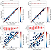 |
Fig. A.1. Comparison between the real injected AGN contribution fraction and the recovered AGN contribution fraction obtained from the Zoobot (top row) and GALFIT (bottom row), for galaxies with low Sérsic index (n < 1; left panels), and high Sérsic index (n > 6; right panels). The colour bar indicates the number of sources in each 2D bin. |
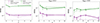 |
Fig. A.2. RMSE as a function of Sérsic index, for the whole sample (top), for galaxies with fAGN < 0.2 (centre), and galaxies with fAGN > 0.8 (bottom). The purple lines correspond to the results from Zoobot, and the green lines from GALFIT. The solid lines correspond to the whole sample, while the dashed and dotted lines correspond to the mergers and non-merger galaxies, respectively. |
Appendix B: AGN example images
We show in Fig. B.1 the 18 galaxies in our sample for which our DL model predicts fAGN > 0.7. These galaxies display a bright central source. In Fig. B.2 and B.3, we show random subsets of X-ray and MIR AGNs, respectively, with a very low fAGN predicted by the model. These galaxies do not show a central component in the F150W filter.
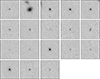 |
Fig. B.1. Example galaxies with fAGN > 0.7. Images are 3.84″across and are displayed with an inverse arcsinh scaling. |
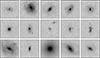 |
Fig. B.2. Example of X-ray AGNs with fAGN < 0.065. Images are 3.84″across and are displayed with an inverse arcsinh scaling. |
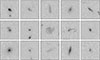 |
Fig. B.3. Example of MIR AGNs with fAGN < 0.065. Images are 3.84″across and are displayed with an inverse arcsinh scaling. |
Appendix C: Colour-colour selection
C.1. Training in multiple JWST filters
We retrained our DL model on mock data constructed for the additional NIRCam filters: F115W, F277W, and F444W. The mock data for these filters were generated analogously to F150W (see Sect. 2.3), with the only differences being the use of the specific filter response curves and PSF models for each band, and the use of cutouts corresponding to the respective filter. The procedure for creating model AGN-host galaxies is identical to that described for F150W (see Sect. 3.1). The training procedure followed the same setup as for F150W (see Sect. 3.2 of the main text), employing the same ConvNeXt-Base architecture pretrained on Zoobot for each dataset.
Table C.1 summarises the model performance in each filter, reporting the RMSE, RAE, mean difference, and outlier fractions (at 20% and 30% thresholds) in the recovery of fAGN across the test sets. The performance is comparable across all filters, indicating that the model is robust to band choice.
Zoobot model performance across JWST filters.
C.2. Application to real JWST data and AGN flux calculation
We applied the trained models to the real JWST/NIRCam data in each filter (F115W, F150W, F277W, and F444W) for the same galaxy sample described in the main text, obtaining a prediction of fAGN in each band. To compute the AGN fluxes, we require total galaxy fluxes, which we adopt from Chen et al., in prep. Briefly, Chen et al. (2025, in prep) used JWST/NIRCam images reduced by Zhuang et al. (2024). The images were processed using JWST pipeline v1.10.2 with CRDS v11.17.0, along with additional custom steps. Source photometry and morphology were derived by modelling each galaxy with a single Sérsic profile using GALFIT (Peng et al. 2002), with initial parameters from SExtractor (Bertin & Arnouts 1996). This process provides both geometric (e.g. axis ratio, position angle) and physical (e.g. flux, magnitude, Sérsic index, effective radius) properties.
The resulting JWST/NIRCam magnitudes were cross-validated against the nearest bands in COSMOS2020 (F115W vs VISTA NB118, F150W vs VISTA H, F277W vs VISTA Ks, and F444W vs IRAC CH2), showing tight correlations and good agreement. The total fluxes are then combined with the fAGN values from our models to derive the nuclear (AGN) fluxes in each band.
C.3. Multi-band analysis
Using the AGN contribution fractions derived in each JWST/NIRCam filter, we performed a multi-band analysis to assess the nature of the central light excess, by constructing colour–colour diagrams in various filter combinations (e.g. F150W–F277W vs F115W–F150W). In Fig. C.1, we show a sub-sample of colour–colour diagrams constructed from the total galaxy fluxes in the four JWST/NIRCam filters.
In each diagram, we show the contours of the non-AGN population (black), defined as galaxies with fAGN < 0.05 in all four filters. The AGN sample is defined as galaxies with fAGN > 5σ in each filter (orange), i.e. systems with a measurable AGN contribution across all bands. We further overplot the MIR-selected AGNs (red), for which fAGN > 5σ in all filters. We focus on this representative sub-sample of colour–colour combinations because they most clearly highlight the systematic differences between the AGN and non-AGN populations. The fAGN-selected AGNs are, on average, redder than the non-AGN galaxies, which may suggest that their host galaxies are more evolved and less actively star-forming, and thus less consistent with young star-forming regions. This reddening could also be driven by the presence of hot dust heated by the AGN, which contributes additional emission at longer wavelengths. The MIR-selected AGNs span a broader range of colours but largely overlap with the fAGN-selected AGNs, often extending towards even redder colours, possibly indicating even higher dust temperatures or more substantial dust obscuration in these systems. To highlight the differences between the non-AGN population and the AGN sample (defined here as galaxies with fAGN > 5σ in each filter), we show, in Fig. C.2, the three colours with the largest median differences between the two populations. These plots also illustrate that the MIR-selected galaxies exhibit more extreme (redder) colours, while our selection tends to identify AGNs whose emission is less distinct from the stellar component, as reflected by their more moderate colours.
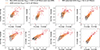 |
Fig. C.1. Colour–colour diagrams for eight representative filter combinations from the four JWST/NIRCam bands (F115W, F150W, F277W, F444W). Black contours show the distribution of non-AGN galaxies (fAGN < 0.05 in all bands). Orange contours indicate the fAGN-selected AGNs based on the whole-galaxy fluxes. MIR-selected AGNs are overplotted as red crosses (if they satisfy fAGN > 5σ). |
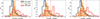 |
Fig. C.2. Normalised colour distributions of our galaxy sample (F115W-F227W, F115W-F444W, and F150W-F444W). Galaxies with negligible nuclear light (fAGN < 0.05 in all filters and not selected as MIR AGNs) are shown in black, AGN candidates with significant nuclear light (fAGN > 5σ in all bands) in orange, and MIR-selected AGNs in red. Vertical lines indicate the median magnitude of each distribution. |
By performing the fAGN analysis across multiple JWST/NIRCam filters, we can partially mitigate the rest-frame wavelength differences introduced by the wide redshift range of our sample (0.5 < z < 3). While any single filter probes different physical regimes at different redshifts, the combination of multiple bands allows us to compare nuclear light excesses more consistently across the sample. This approach reduces, though does not fully eliminate, potential biases due to varying SED coverage. A more detailed analysis accounting explicitly for rest-frame band differences and nuclear versus host SEDs will be required to fully quantify these effects.
All Tables
All Figures
|
Fig. 1. Overview of the JWST/NIRCam F150W PSFs in COSMOS-Web. We stacked all available PSFs from Zhuang et al. (2024) and show the mean PSF (left), standard deviation (centre), and the coefficient of variation (right), calculated pixel by pixel. The PSFs have been re-binned to a pixel resolution of 0.03 ″/pixel, matching the resolution used for the synthetic image creation. The axes show the number of pixels, corresponding to 3″across. The colour bar shows the value of each pixel. |
| In the text | |
|
Fig. 2. Example mock JWST/NIRCam F150W images with varying levels of AGN contribution. The images have been generated to mimic JWST observations and include realistic JWST noise and background. Each row corresponds to a different galaxy, with no AGN contribution in the left panel and increasing AGN contributions in the rest of the panels. We show four example galaxies with different magnitudes, from the brightest (top) to the faintest (bottom). Images are 3.84″across and are displayed with an inverse arcsinh scaling. |
| In the text | |
|
Fig. 3. Architecture of ConvNeXt-Base network (bottom) with a four-stage feature hierarchy, which allows us to extract features on different scales. On top of each stage, we show the dimension of the feature maps, with the width and height decreasing as the network deepens, while the filter size increases. The top left diagram shows the internal structure of ConvNeXt Block. The top right diagram shows the internal structure of Downsample. The LN and GELU represent a layer normalisation and a Gaussian error linear unit activation function, respectively. |
| In the text | |
|
Fig. 4. Distributions of the injected AGN contribution fraction (as defined in Eq. (8)) in the training (blue) and test datasets (orange). The distributions are mostly uniform for both the training and test datasets. |
| In the text | |
|
Fig. 5. Sérsic + PSF decomposition of four example galaxies (with AGN contribution fraction varying from high to low from top to bottom) on which we performed GALFIT. Images of the original galaxy, the model (Sérsic + PSF), and the residual (original−model) are shown from left to right. Images are 3.84″across and are displayed with an inverse arcsinh scaling. |
| In the text | |
|
Fig. 6. Comparison between the real injected AGN contribution fraction and the AGN contribution fraction obtained from the Zoobot model on the subset of 4800 galaxies across the whole redshift range (0.5 < z < 3). The comparison shows a mean difference between the two quantities (ΔfAGN = fAGN [Injected] −fAGN [Zoobot]) of −0.0018 and an overall RMSE = 0.013. The solid diagonal line is the 1:1 line. The top plot shows the mean difference and its dispersion as a function of the injected AGN contribution fraction. The colour bar indicates the number of sources in each bin. |
| In the text | |
|
Fig. 7. RMSE as a function of the injected AGN contribution fraction (top left), redshift (top right), S/N (bottom left), and rkron (bottom right). The purple lines correspond to the results from Zoobot, and the green lines from GALFIT. The solid lines correspond to the whole sample, while the dashed and dotted lines correspond to the mergers and non-merger galaxies, respectively. The error bars show the 95% interval from bootstrapping the RMSE value. The performance of Zoobot is around a factor of ten better than GALFIT. The shaded region in the top left panel represents the fractional variation (standard deviation divided by the mean) of the PSF, considering the spatial and temporal variations. |
| In the text | |
|
Fig. 8. Average RAE in bins of injected fAGN (top left), redshift (top right), S/N (bottom left), and rkron (bottom right), from the Zoobot predictions. The error bars correspond to the standard deviation of the data points in each bin. The purple lines correspond to the results from Zoobot, and the green, from GALFIT. The solid lines correspond to the whole sample, while the dashed and dotted lines correspond to the merger and non-merger galaxies, respectively. |
| In the text | |
|
Fig. 9. Outlier fraction (calculated as the fraction of galaxies with RAE > 20%) as a function of the injected AGN contribution fraction (top left), redshift (top right), S/N (bottom left), and rkron (bottom right). The purple lines correspond to the results from Zoobot, and the green, from GALFIT. The solid lines correspond to the whole sample, while the dashed and dotted lines correspond to the merger and non-merger galaxies, respectively. |
| In the text | |
|
Fig. 10. Comparison between the real injected AGN contribution fraction and the AGN contribution fraction obtained from GALFIT fitting, obtained by dividing the PSF flux by the total flux. Left: Total flux corresponds to the flux measured within a 2″aperture in the original image. Right: Flux measured within a 2″aperture in the model (Sérsic+PSF). In both cases, the PSF flux was measured within the same aperture in the model PSF image. The dispersion in the left panel corresponds to RMSE = 0.12, and in the right, RMSE = 0.17. The colour bar provides the number of sources in each 2D bin. |
| In the text | |
|
Fig. 11. Number of galaxies for which GALFIT returns a good fit (blue histograms) and for which there is a bad fit or no fit from GALFIT (red histograms), as a function of the injected AGN contribution fraction (top left), redshift (top right), S/N (bottom left), and rkron (bottom right). GALFIT tends to fail for bright galaxies, galaxies with low S/N, or with very high or low injected AGN contribution fractions. |
| In the text | |
|
Fig. 12. Distribution of the predicted fAGN on the sample of JWST galaxies (purple). The blue and red histograms show the predictions for the X-ray and MIR AGNs within our sample, respectively. The black line (fAGN = 0.065) represents the 5σ value with respect to the overall mean RMSE. The x and y axes are displayed on a logarithmic scale. |
| In the text | |
|
Fig. 13. Fraction of galaxies in bins of predicted AGN contribution fraction in the X-ray AGNs, MIR AGNs, and ’non-AGNs’ samples. |
| In the text | |
|
Fig. 14. Top: Overlapping fraction of AGNs also identified by our DL method as a function of the adopted cut on the X-ray or the rest-frame 6 μm luminosity for the X-ray and MIR-selected AGNs. The solid lines show the overlapping fraction by applying a cut at fAGN > 0.2, while the dashed lines show the overlapping fraction if we select AGNs by requiring fAGN > 0.1. Bottom: AGN luminosity in the JWST/NIRCam F150W filter versus the X-ray luminosity or the rest-frame 6 μm luminosity, for the X-ray-selected or MIR-selected AGNs. The dash-dotted lines show the respective linear fits. |
| In the text | |
|
Fig. A.1. Comparison between the real injected AGN contribution fraction and the recovered AGN contribution fraction obtained from the Zoobot (top row) and GALFIT (bottom row), for galaxies with low Sérsic index (n < 1; left panels), and high Sérsic index (n > 6; right panels). The colour bar indicates the number of sources in each 2D bin. |
| In the text | |
|
Fig. A.2. RMSE as a function of Sérsic index, for the whole sample (top), for galaxies with fAGN < 0.2 (centre), and galaxies with fAGN > 0.8 (bottom). The purple lines correspond to the results from Zoobot, and the green lines from GALFIT. The solid lines correspond to the whole sample, while the dashed and dotted lines correspond to the mergers and non-merger galaxies, respectively. |
| In the text | |
|
Fig. B.1. Example galaxies with fAGN > 0.7. Images are 3.84″across and are displayed with an inverse arcsinh scaling. |
| In the text | |
|
Fig. B.2. Example of X-ray AGNs with fAGN < 0.065. Images are 3.84″across and are displayed with an inverse arcsinh scaling. |
| In the text | |
|
Fig. B.3. Example of MIR AGNs with fAGN < 0.065. Images are 3.84″across and are displayed with an inverse arcsinh scaling. |
| In the text | |
|
Fig. C.1. Colour–colour diagrams for eight representative filter combinations from the four JWST/NIRCam bands (F115W, F150W, F277W, F444W). Black contours show the distribution of non-AGN galaxies (fAGN < 0.05 in all bands). Orange contours indicate the fAGN-selected AGNs based on the whole-galaxy fluxes. MIR-selected AGNs are overplotted as red crosses (if they satisfy fAGN > 5σ). |
| In the text | |
|
Fig. C.2. Normalised colour distributions of our galaxy sample (F115W-F227W, F115W-F444W, and F150W-F444W). Galaxies with negligible nuclear light (fAGN < 0.05 in all filters and not selected as MIR AGNs) are shown in black, AGN candidates with significant nuclear light (fAGN > 5σ in all bands) in orange, and MIR-selected AGNs in red. Vertical lines indicate the median magnitude of each distribution. |
| In the text | |
Current usage metrics show cumulative count of Article Views (full-text article views including HTML views, PDF and ePub downloads, according to the available data) and Abstracts Views on Vision4Press platform.
Data correspond to usage on the plateform after 2015. The current usage metrics is available 48-96 hours after online publication and is updated daily on week days.
Initial download of the metrics may take a while.