| Issue |
A&A
Volume 706, February 2026
|
|
|---|---|---|
| Article Number | A206 | |
| Number of page(s) | 19 | |
| Section | Extragalactic astronomy | |
| DOI | https://doi.org/10.1051/0004-6361/202555047 | |
| Published online | 10 February 2026 | |
The Atacama Cosmology Telescope: Observations of supermassive black hole binary candidates
Strong sinusoidal variations at 95, 147, and 225 GHz in PKS 2131–021 and PKS J0805–0111
1
David A. Dunlap Department of Astronomy & Astrophysics, University of Toronto 50 St. George St. Toronto ON M5S 3H4, Canada
2
Specola Vaticana (Vatican Observatory) V-00120 Vatican City, Vatican City State
3
Kavli Institute for Astronomy & Astrophysics, Peking University Beijing 100871, People’s Republic of China
4
Department of Astronomy, School of Physics, Peking University Beijing 100871, People’s Republic of China
5
Astronomical Observatory, University of Warsaw Al. Ujazdowskie 4 00-478 Warszawa, Poland
6
Institute of Theoretical Astrophysics University of Oslo, Norway
7
Institute of Astrophysics, Foundation for Research & Technology-Hellas GR-71110 Heraklion, Greece
8
Kavli Institute for Particle Astrophysics and Cosmology, Department of Physics, Stanford University Stanford CA 94305, USA
9
Canadian Institute for Theoretical Astrophysics, University of Toronto 60 St. George Street Toronto ON M5S 3H8, Canada
10
Department of Physics & Astronomy, University of Pennsylvania 209 South 33rd Street Philadelphia PA 19104, USA
11
Joseph Henry Laboratories of Physics, Jadwin Hall, Princeton University Princeton NJ 08544, USA
12
Department of Astrophysical Sciences, Peyton Hall, Princeton University Princeton NJ 08544, USA
13
Division of Physics, Mathematics, and Astronomy, California Institute of Technology Pasadena CA 91125, USA
14
Dunlap Institute for Astronomy & Astrophysics, University of Toronto 50 St. George St. Toronto ON M5S 3H4, Canada
15
Instituto de Astrofísica & Centro de Astro-Ingeniería, Facultad de Física, Pontificia Universidad Católica de Chile Av. Vicuña Mackenna 4860 7820436 Macul Santiago, Chile
16
Department of Astronomy & Astrophysics, University of Chicago 5640 South Ellis Avenue Chicago IL 60637, USA
17
Department of Physics and Astronomy, University of Pittsburgh 3941 O’Hara Street Pittsburgh PA 15260, USA
18
TAPIR, Mailcode 350-17, California Institute of Technology Pasadena CA 91125, USA
19
Walter Burke Institute for Theoretical Physics, California Institute of Technology Pasadena CA 91125, USA
20
Department of Physics, Cornell University Ithaca NY 14853, USA
21
Department of Astronomy, Cornell University Ithaca NY 14853, USA
22
Department of Physics & Astronomy, Haverford College Haverford PA 19041, USA
23
Owens Valley Radio Observatory, California Institute of Technology Pasadena CA 91125, USA
24
Instituto de Física, Pontificia Universidad Católica de Valparaíso Casilla 4059 Valparaíso, Chile
25
Mitchell Institute for Fundamental Physics & Astronomy and Department of Physics & Astronomy, Texas A&M University College Station TX 77843, USA
★ Corresponding author: This email address is being protected from spambots. You need JavaScript enabled to view it.
Received:
4
April
2025
Accepted:
8
December
2025
Abstract
Large sinusoidal variations in the radio light curves of the blazars PKS J0805–0111 and PKS 2131–021 have recently been discovered with an 18-year monitoring programme at the Owens Valley Radio Observatory, making these systems strong supermassive black hole binary (SMBHB) candidates. The sinusoidal variations in PKS 2131–021 dominate its light curves from 2.7 GHz to optical frequencies. We report sinusoidal variations observed in both objects with the Atacama Cosmology Telescope (ACT) at 95, 147, and 225 GHz consistent with the radio light curves. The ACT 95 GHz light curve of PKS 2131–021 agrees well with the contemporaneous 91.5 GHz ALMA light curve and is comparable in quality, while the ACT light curves of PKS J0805–0111, for which there are no ALMA or other millimetre light curves, show that PKS 2131–021 is not an isolated case, and that this class of AGN exhibits the following properties: (a) the sinusoidal pattern dominates over a broad range of frequencies; (b) the amplitude of the sine wave compared to its mean value is monochromatic (i.e. nearly constant across frequencies); (c) the phase of the sinusoid phase changes monotonically as a function of frequency; (d) the sinusoidal variations are intermittent. We describe a physical model for SMBHB systems, the modified Kinetic Orbital model, that explains all four of these phenomena. The monitoring of ∼8000 blazars by the Simons Observatory over the next decade should provide a large number of SMBHB candidates that will shed light on the nature of the nanohertz gravitational-wave background.
Key words: galaxies: active / galaxies: jets / quasars: supermassive black holes
© The Authors 2026
 Open Access article, published by EDP Sciences, under the terms of the Creative Commons Attribution License (https://creativecommons.org/licenses/by/4.0), which permits unrestricted use, distribution, and reproduction in any medium, provided the original work is properly cited.
This article is published in open access under the Subscribe to Open model. This email address is being protected from spambots. You need JavaScript enabled to view it. to support open access publication.
1. Introduction
Evidence of a stochastic background of gravitational waves with periods of months to years has recently been presented by the North American Nanohertz Observatory for Gravitational Waves collaboration (Agazie et al. 2023a) and the European Pulsar Timing Array collaboration (EPTA Collaboration 2023). The MeerKAT Pulsar Timing Array collaboration also find evidence of the background, but caution that it is highly dependent on the choices in their noise modelling (Miles et al. 2025). These experiments use millisecond pulsar timing arrays (Readhead & Hewish 1974; Backer et al. 1982)1, which currently provide the most sensitive method of searching for gravitational waves at these frequencies, although stellar astrometry of billions of stars (e.g. Moore et al. 2017; Braginsky et al. 1990) may be competitive in the future. Supermassive black hole binary systems (SMBHBs) have been suggested as the origin of this stochastic background (e.g. Agazie et al. 2023a,b), making clear the importance of searches for their electromagnetic counterparts.
Supermassive black holes (SMBHs) are the central engines in active galactic nuclei (AGN), which are strong sources of emission across the electromagnetic spectrum (Krolik & Di Matteo 2000; Blandford et al. 2019). Since 2008 the 40 m Telescope of the Owens Valley Radio Observatory (OVRO) has been dedicated full time to monitoring ∼1830 blazars at 15 GHz on a 3–4 day cadence (Richards et al. 2011). Of the ∼1830 blazars monitored, 1158 comprise a complete sample suitable for statistical tests. To date, two AGN with sinusoidal variations dominating their light curves have been identified in this sample, which rigorous statistical tests show are unlikely to be produced by random fluctuations in the red noise tail of their power spectral density: PKS 2131–021 (O’Neill et al. 2022, hereafter referred to as O22; Kiehlmann et al. 2025, hereafter K25) and PKS J0805–0111 (de la Parra et al. 2025, hereafter D25)2. K25 and D25 simulated 106 light curves that match the power spectral densities and probability density functions (i.e. the flux distribution) of PKS 2131–021 and PKS J0805–0111, and show that the joint global probability, p, of these two sources, out of the sample of 1158, being generated randomly due to the red noise tail in their variability spectra is p < 3 × 10⁻³ (D25). Ren et al. (2021b) and Ren et al. (2021a) were the first to draw attention to possible quasi-periodic oscillations in PKS J0805–0111 and PKS 2131–021, respectively. However, in the case of PKS J0805–0111, D25 argue that they overestimated the significance of the periodicity by several orders of magnitude by assuming the data consisted of independent Gaussian values; similarly, for PKS 2131–021, the reported significance of the periodicity is inflated since they consider the local rather than the global significance (cf. O22).
It is by no means obvious that orbital motion of a SMBH with a relativistic jet will produce sinusoidal variations; however, a mechanism was discovered independently by Sobacchi et al. (2017) and by O22, which K25 refer to as the Kinetic Orbital (KO) model. In the KO model, one of the SMBHs in the binary system produces a jet, and the aberration of this jet due to orbital motion has a large effect on the observed emission from the highly relativistic emitting material. This is shown in O22 to produce sinusoidal variations. While other mechanisms, for example oscillations or precessions in the accretion disc, have been invoked to explain (quasi-)periodic behaviour in AGN light curves (see e.g. discussions in O22; An et al. 2013; Wang et al. 2014; Ingram & Motta 2019), the KO model is remarkably simple and economically explains the relevant observed phenomena.
In addition to studying radio light curves, K25 analysed publicly available light curves of PKS 2131–021 at millimetre (mm), infrared, and optical frequencies and found the same sine wave pattern in them all, as well as ‘hints’ (as they put it) of a sinusoid at γ-ray frequencies. This broad-band signal is explained well by the KO model since the orbital aberration affects all frequencies. The light curves exhibit a monotonic phase shift in the sine waves from the radio to the optical, spanning more than five decades in frequency. This can be interpreted as an optical depth effect in which the higher frequencies probe closer to the central engine, a behaviour that has been observed in many blazars since it was discovered in the first maps made with very long baseline interferometry (VLBI; Readhead et al. 1978; Readhead 1980). In the KO model, simultaneous observations of multiple frequencies capture the jet at different points along its helical structure, and thus at different phases of the orbital pattern. Although the light travel time between the higher-frequency and lower-frequency zones corresponds to several sinusoidal cycles, the jet itself is travelling at close to the speed of light. Therefore, by the time the higher-frequency light arrives at the location of the lower-frequency emission, the jet material lags behind only slightly, leading to a relatively small phase delay in the observed light curve. An issue with this model, however, is that it is unclear how the helical structure can remain coherent over a large number of windings spanning tens of parsecs.
In this paper we report observations made with the Atacama Cosmology Telescope (ACT) of PKS 2131–021 and PKS J0805–0111 from 2016 to 2022 at 95, 147, and 225 GHz that provide new insights into these two objects and the phenomenology of SMBHBs in blazars. Furthermore, we present a modified KO (MKO) model that solves the problem of maintaining a helical structure of the jet over hundreds of orbital periods by proposing that a sub-relativistic wind, which is dragged by the SMBH orbit, confines the relativistic flow of the jet and results in a helix that need not span so many windings to explain the observations. This model is presented in more detail by Sullivan et al. (2025). We also review recent numerical simulations of accretion discs that show how the jet can be interrupted in such a way as to produce the observed intermittency of the sinusoidal pattern in the light curves. Finally, we discuss the potential for wide-field CMB surveys to discover scores of SMBHB candidates and determine their periods, which has implications for gravitational wave science and SMBHB population studies.
The paper is organised as follows. In Sect. 2 we describe the ACT light curves and briefly introduce other key data used in our analyses. In Sect. 3 we present sinusoidal fits to the ACT light curves of PKS 2131–021 and PKS J0805–0111, and in Sect. 4 we analyse and discuss the relative phase shifts between light curves at different frequencies as well as the achromaticity of the sinusoidal amplitudes. In Sect. 5 we present the MKO model and outline the relevance of recent numerical simulations of accretion discs for SMBHB blazars. In Sect. 6 we discuss the promise of mm observations of AGN for future SMBHB candidate discoveries, comparing and contrasting to optical searches. We summarise our findings and discuss the potential of upcoming mm surveys for discovering SMBHB candidates in Sect. 7.
2. Data
2.1. The ACT observations
ACT was a cosmic microwave background (CMB) experiment that operated from 2007 to 2022 in the Atacama Desert of Chile. Its 6 m telescope observed with three generations of receivers: the Millimeter Bolometric Array Camera (MBAC, 2007–11; Swetz et al. 2011), ACTPol (2013–15; Thornton et al. 2016) and Advanced ACTPol (2016–22; Henderson et al. 2016). All receivers were equipped with three optics tubes, each terminating in its own array of detectors that were occasionally changed to allow different combinations of frequencies to be observed. Starting with ACTPol, detectors were polarisation-sensitive and, beginning with the fourth polarised array (PA4), were also dichroic, i.e. sensitive to two frequency bands. Collectively, PA1 to PA7 observed in five frequency bands: f030, f040, f090, f150, and f220. The two lowest frequencies are still being analysed, and all science results so far, including in this paper, come from f090, f150, and f220, whose band centres for a synchrotron spectral index of −0.7, averaged across the PAs, were 95.0, 147.1, and 225.0 GHz, respectively3 (see Hervías-Caimapo et al. 2024 for a full summary of the array timelines and frequencies). The passbands are discussed in Madhavacheril et al. (2020) and Coulton et al. (2024).
A paper presenting the ACT bright AGN sample is in preparation (Ma et al., in prep.), and the light curve data will be publicly released. The data reduction process and an analysis of calibration uncertainties and other error sources will be described more fully in that paper and here we introduce only the essentials. Light curves were generated by creating 2 × 2 deg2 maps centred on the source for each day the source was observed. Data were calibrated from raw readout units to incident power by measuring the detector response to small, square-wave changes in the voltage bias applied to the detectors (Niemack 2008); this was performed at least hourly. Interdetector calibration was achieved by flat fielding on the atmospheric emission which creates a common signal mode across the detectors. Calibration from incident power to celestial flux density was achieved using observations of Uranus that were taken every few nights and a final correction based on cross correlating ACT and Planck angular power spectra was applied4 (see Choi et al. 2020 and Naess et al. 2025 for more information on the general map-making process). With the individual maps in hand, the point source flux density was extracted from each with a matched filter using the known telescope beams and a noise covariance estimated from the map itself after masking the source, similar to the method of Marriage et al. (2011), except that individual pixel weights were also accounted for in the noise covariance5. The resulting light curves tended to have a few outlying points, almost all of which were automatically flagged as outliers by our pipeline due to the low effective number of detectors in the receiver for a particular observation (e.g. because of bad weather, or because the source was near the edge of the observed field). A small fraction of data points, ∼0.1%, were flagged as outliers based on conservative visual inspections. In this work we excluded all points flagged as outliers and we combined all light curves from different polarised arrays that were observed at the same frequency (e.g. PA3–f090, PA5–f090 and PA6–f090).
Ma et al. will provide a detailed uncertainty analysis of the calibration, but preliminary studies of the variance of Uranus measurements over time, as well as comparison of flux densities of the AGN between array-bands (e.g. PA5–f090 vs. PA6–f090), indicate an uncertainty of ∼2 to 7%, depending on the array-frequency channel (cf. Hervías-Caimapo et al. 2024). These systematic measurement errors, which are not Gaussian-distributed, cause point-to-point scatter in the light curves that is mixed in with any intrinsic variability of observed sources. However, the results of this paper do not rely on detailed knowledge of these sources of uncertainty.
2.2. Key Data at Other Wavelengths
Our analysis included the following light curves from other observatories that overlap in time with the ACT light curves:
-
OVRO light curves of PKS 2131–021 and PKS J0805–0111 at 15 GHz (Richards et al. 2011).
-
Atacama Large Millimeter Array (ALMA) light curves of PKS 2131–021 at 91.5, 103, 104, 337, 343, 344, 349, and 350 GHz, taken from the ALMA Calibrator Source Catalogue6. Following K25, we combined the 103 and 104 GHz data into a single light curve and call the combination ‘103.5 GHz’. We also combined 337–350 GHz and refer to it as ‘345 GHz’.
-
The Catalina Real Time Survey (CRTS; Drake et al. 2009) light curve of PKS 2131–021 in the optical V-band.
-
The Zwicky Transient Facility (ZTF; Masci et al. 2019; Graham et al. 2019) light curve of PKS 2131–021 in the optical g-band.
Data from CRTS and ZTF were re-binned to a daily cadence using a weighted mean scheme. For consistency with K25, especially in our analysis of the sinusoid phase shifts (Sect. 4.1), we used the same time spans as they did: MJD 56647.1–60053.7 (21 December 2013–19 April 2023) for the ALMA light curves, and MJD 54470.9–60175.3 (5 January 2008–19 August 2023) for OVRO.
The redshifts of PKS 2131–021 and PKS J0805–0111 are 1.285 and 1.39, respectively (Drinkwater et al. 1997; Paliya et al. 2017).
3. Sine-wave fits to the light curves
3.1. Method
We fitted a sine wave function to the OVRO and ACT data by maximising the following likelihood function:
![Mathematical equation: $$ \begin{aligned} \ln \mathcal{L}&= -\frac{1}{2}\sum _{j = 1}^4\sum _{i = 1}^{N_j} \frac{\left(S_{ij}-\bar{S}_j-A_j \sin \left[\frac{2\pi }{P}(t_{ij} - t_0)-\phi _j\right]\right)^2}{\sigma _{ij}^2+\xi _j^2} \nonumber \\&\quad -\frac{1}{2}\sum _{j = 1}^4\sum _{i = 1}^{N_j}\ln (\sigma _{ij}^2+\xi _j^2), \end{aligned} $$](/articles/aa/full_html/2026/02/aa55047-25/aa55047-25-eq1.gif) (1)
(1)
where i is the time index of the light curve and j stands for each of the light curves: OVRO 15 GHz, ACT 95 GHz, ACT 147 GHz, and ACT 225 GHz, respectively. The light curves, Sij, which have Nj points and uncertainties σij, are sampled at times tij; the reference time for the sinusoid phase was set at t0= MJD 59 000 (2020 May 31). The period, P, was held fixed during the fit (see below), and there were four free parameters per light curve: the sine-wave offset  , amplitude Aj, and phase ϕj, plus a term quantifying the correlated noise in the data, ξj.
We determined the period P by fitting the OVRO data alone in the range where there are ACT data. Then, keeping this period fixed, we did the joint fit of Eq. (1) described above. The reason for calculating the period only within the ∼6-year time range where there are ACT data, rather than over the whole range of the OVRO data, was that real flux fluctuations due to processes inside the jet, which are superimposed on the sinusoidal signal, act as a source of ‘noise’ in the sine-wave fits that may not be fully captured by the correlated noise term ξ, and would require more SMBHB candidates to be properly understood. See O22, K25 and Appendix C.1 for a more detailed discussion of this source of uncertainty. Restricting the fit to the time range when both OVRO and ACT data exist was the best approach for measuring the phase shifts as a function of frequency (see Sect. 4.1). A result of this restriction of the time range is that the fits with ACT and ALMA data have slightly different fixed periods (≈4%), since their time spans are not equivalent (see Fig. 1 and compare Tables 1 and B.1).
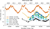 |
Fig. 1. PKS 2131–021 light curves from OVRO, ACT, and ALMA. Heavy points are binned into 50-day intervals (100 for OVRO) to guide the eye, with individual measurements shown as lighter points. Sinusoidal fits, shown with the continuous curves, were done on the unbinned data. The sine fits for ALMA are from K25 and sine fits to ACT were done for this paper (see text). For the OVRO data, the solid curve is the best fit for the ACT time range, while the dashed sine curve corresponds to the ALMA time range. A monotonic phase shift of the sine waves to earlier times with increasing frequency is visible by eye, and is reported relative to the OVRO phase as Δϕ0 in Tables 1 and B.1. |
The best-fitting parameters and their uncertainties were calculated with a Markov chain Monte Carlo (MCMC) using the EMCEE code (Foreman-Mackey et al. 2013). The phase shifts were calculated from the best-fitting values as
 (2)
(2)
The uncertainties represent the 68% confidence range of the marginalised posterior distributions. The results of the fits are reported in Tables 1 and 2; the fits to the OVRO + ALMA data, which are the same as those presented in K25 and were performed with the same methodology described above, are given in Table B.1.
Sine-wave fit results for PKS 2131–021.
Sine-wave fit results for PKS J0805–0111.
3.2. The light curves of PKS 2131–021
It is fortunate that PKS 2131–0217 is an ALMA calibrator that was observed during the same time period as the ACT data, as it affords us the opportunity to compare the ACT 95 GHz light curve with ALMA at 91.5 and 103.5 GHz, providing a useful cross-check of the calibration of the ACT data. The ACT light curves of PKS 2131–021 at 95, 147, and 225 GHz are shown in Fig. 1, together with the OVRO 15 GHz and ALMA 91.5 GHz and 345 GHz light curves.
The ACT 95 GHz data show good consistency with the ALMA 91.5 GHz and 103.5 GHz data. We determined this by comparing the ratio of their light curves after colour-correcting the ALMA data to the ACT band centre using a spectral index of −0.38 ± 0.12, which we obtained from the ratio of the ALMA 91.5 GHz and 103.5 GHz data for the 219 instances where both bands had simultaneous measurements8. The mean ratio of the 95 GHz ACT flux to the 91.5 ALMA flux, using the 30 pairs of data points measured on the same day in both experiments, is 1.01 ± 0.04. For ACT 95 GHz and ALMA 103.5 GHz, the mean ratio is 1.00 ± 0.05, using the 28 available pairs of data. Another comparison, albeit less precise, can be made using the ratio of the best-fitting sinusoid offsets,  . After colour correcting these offsets, we find: 1.00 ± 0.12 for ACT 95 GHz vs. ALMA 91.5 GHz, and 1.00 ± 0.13 for ACT 95 GHz vs. ALMA 103.5 GHz. We note that the uncertainties here are dominated by the uncertainty in colour correction. Farren et al. (2021) also find consistency between ACT and ALMA flux densities using a few dozen point sources. In their case, the comparison is between ACT fluxes averaged over a year and ALMA data from the same year, rather than between individual points in light curves as we have done here, which they note increases the measurement uncertainty.
A further agreement between ACT and ALMA is found in the scatter in their light curves, which is similar between the two datasets on ∼month-long timescales. This ‘scatter’ is actually due to real flux density variations in the source. We illustrate this in the top panel of Fig. 2, in which the long-term sinusoidal variation of the ALMA and ACT light curves has been filtered out and the two resulting light curves exhibit similar residuals. The bottom panel shows the Pearson correlation between the ALMA 91.5 GHz and ACT 95 GHz data as a function of how aggressive this high-pass filter is. On timescales > 1 month the level of correlation is significant; on shorter timescales the correlation is noise dominated.
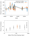 |
Fig. 2. Correlation of medium-term flux density variations in ALMA and ACT light curves of PKS 2131–021. Top: ALMA 91.5 GHz and ACT 95 GHz (PA5) light curves that have been filtered by binning and subtracting a long timescale trend. The binning is in five day chunks, and only time chunks containing data from both ALMA and ACT are retained. The long timescale trend was removed by fitting a third-degree B-spline with 120-day knot spacing to each binned light curve and subtracting; this effectively acts as a high-pass filter of variations on timescales ≳120 days, removing the large sinusoidal pattern. Clear correlations between the light curves are seen on these timescales. Bottom: Pearson correlation between the filtered ALMA and ACT light curves, for different spline knot spacings. Errors were estimated by calculating the correlations between the ALMA PKS 2131–021 light curve and each of the other 204 ACT light curves in our bright AGN library, which should be uncorrelated, and taking the standard deviation. The thick coloured point at 120 days corresponds to the data shown in the upper panel. |
In Fig. 1 we see a monotonic progression of the phases of the fitted sine waves with observing frequency, with the higher frequencies leading the lower frequencies. This phenomenon was discovered by K25. Ren et al. (2025) also explored phase shifts in PKS 2131–021 using radio (OVRO), infrared (WISE and NEOWISE) and optical (ZTF, CRTS, and Asteroid Terrestrial-impact Last Alert System) light curves. They find phase shifts of −0.19 ± 0.13 cycles between radio and infrared and −0.17 ± 0.13 cycles between radio and optical9. Since their results come from cross-correlation the uncertainties are much larger than K25 but are consistent within the error bars. We analyse the phase shifts later, in Sect. 4.1.
3.3. The ACT light curve of PKS J0805–0111
We now turn to the case of PKS J0805–0111, for which there are no ALMA data. This is the second OVRO blazar discovered to exhibit significant sinusoidal variations, thereby making it a strong SMBHB candidate (D25). Best-fitting sinusoids to the ACT and OVRO data are reported in Table 2 and are shown along with the light curves in Fig. 3. The sinusoidal variation discovered at 15 GHz in the OVRO light curve of PKS J0805–0111, which lasted from 2008 to 2020 (D25), is clearly also seen in the ACT light curves, and shows that the broad-band sinusoidal variation seen in PKS 2131–021 is not simply an isolated case. It suggests that broad-band sinusoidal emission is a common phenomenon in SMBHB blazar candidates. The KO model explains this phenomenology which has now been confirmed in our two high-significance SMBHB candidates. This could be important for the detection of gravitational waves from SMBHBs.
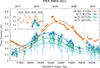 |
Fig. 3. PKS J0805–0111 light curves at 15 GHz, 95 GHz, 147 GHz, and 225 GHz. The main panel shows the time range covered by the ACT observations, while the inset shows the full range observed by OVRO. Heavy points are binned into 25-day intervals (100 days in the inset) to guide the eye, with individual measurements shown as lighter points; the sinusoidal least-squares fits were done on the unbinned data. A monotonic phase shift of the sine waves to earlier times with increasing frequency is visible by eye, and is reported relative to the OVRO phase as Δϕ0 in Table 2. The dashed vertical line at MJD 59041 (2020 July 11) indicates the approximate date at which D25 found that the sinusoidal variation in the 15 GHz ceases. The ACT mm data also apparently flatten around the same time. |
D25 found that the sinusoidal variations in the 15 GHz OVRO light curve ceased at around MJD 59041, shown in Fig. 3 with a dashed, vertical line. Although the ACT light curves do not extend long after this date, they too appear consistent with the sinusoid shutting off. A similar phenomenon is also observed by O22 and K25 in PKS 2131–021 in more than 45 years of data: its light curve is sinusoidal for about the first seven years, then non-sinusoidal for 19 years, after which the sinusoid recommences with a smaller amplitude but otherwise consistent, in both period and phase, with the original periodicity. Completely independent fits to the Haystack data (1975–1983) and to the OVRO data (2008–2020) give periods of 1729.1 ± 32.4 days and 1760 ± 5.3 days, respectively (O22). This is the same period within the uncertainties, which is better than 2%. Moreover, the new sinusoid is in phase with the original to within ∼10% of a cycle (O22). This suggests that the underlying mechanism is a good clock, i.e. the SMBHB orbit according to the KO model, that continued running when the sinusoidal variation seen in the Haystack and OVRO data was absent. The temporary cessation of the sinusoid is not explained by KO model per se, but O22 and K25 point out that its disappearance, as well as the change in its amplitude when it reappears, could plausibly be produced by changes in the fuelling of the jet. We discuss this intermittency in more detail in Sect. 5.2.
As in the case of PKS 2131–021, a monotonic phase shift with frequency is observed in the light curves, which we analyse in Sect. 4.1.
4. Multi-frequency properties of the SMBHB candidates
4.1. Frequency-dependent phase shifts
As noted in the previous section, in both of our sources the higher-frequency ACT light curves are shifted towards earlier times relative to the OVRO 15 GHz light curves, and the shift is monotonic with frequency. This behaviour is explained by the KO model as being due to frequencies originating at different positions along the jet because of optical depth effects, and is further discussed below in the context of our new MKO model (Sect. 5.1).
Table 3 shows the phase shifts for PKS 2131–021. In addition to the phase shifts of the ACT light curves relative to OVRO, it includes the phase shifts of light curves from the Haystack observatory (radio), ALMA (mm), the Wide-field Infrared Survey Explorer (WISE; infrared), and ZTF (optical), all relative to OVRO, as listed in Table 2 of K25. We note that the Haystack data come from an earlier time period (1975–1983) and do not overlap with the other datasets; thus, the phase shifts for the Haystack light curves are relative to the 15.5 GHz Haystack channel. The coherent behaviour from 2.7 GHz to optical wavelengths is strikingly illustrated by Fig. 4, which shows the phase shift measurements overplotted on the best-fit quadratic phase–frequency relation from K25:
PKS 2131–021 phase shifts with frequency.
![Mathematical equation: $$ \begin{aligned} \Delta \phi = 0.178 - 0.146\log _{10}(\nu ) + 0.0093[\log _{10}(\nu )]^2. \end{aligned} $$](/articles/aa/full_html/2026/02/aa55047-25/aa55047-25-eq7.gif) (3)
(3)
We discuss these phase shifts and Eq. (3) shortly.
Table 4 lists the phase shifts for PKS J0805–0111. We note that, as found in PKS 2131–021, the ACT sinusoids are shifted towards earlier times relative to the OVRO 15 GHz light curve, and the shift is consistent with being monotonic with frequency. This is therefore likely to be a common phenomenology in SMBHB blazar candidates and a signature of a fundamental property of these jets.
PKS J0805–0111 phase shifts with frequency relative to the 15 GHz light curve.
The exact form of the frequency phase–shift relation depends on the details of where different frequencies originate in the blazar jet. The simple quadratic fit by K25 to the PKS 2131–021 phase shifts (Eq. (3)) is not motivated by any particular jet model but is purely phenomenological. While the ACT 95 GHz measurement agrees with this curve, and is consistent with the ALMA measurement, the 147 GHz and 225 GHz measurements are 3.1σ and 1.2σ higher than the curve, respectively. A power law is potentially more physically realistic:
 (4)
(4)
Here a and b are model parameters and ν0 is the reference frequency for the phase shifts, in our case 15 GHz. This equation is motivated by the theoretical prediction that the distance along the jet of the emission zone goes as r ∝ ν−1 when the jet is optically thick (Blandford & Königl 1979). Equation (4) follows because the phase shift in the KO model is due to light-travel times, and thus proportional to r. Figure 4 shows the best fit of Eq. (4) to the radio and mm data (Haystack, ALMA, and ACT) for PKS 2131–021, with best-fitting parameters reported in Table 510. Fits were performed with a Metropolis–Hastings Monte Carlo (MC) with flat priors in the ranges b = (0.05, 4) and a = ( − 2, −0.05). The priors were cut off before zero to prevent the MC from piling up near unphysical a = 0. The exact cutoff does not change the maximum likelihood; naturally, though, it alters the posterior credible regions that we use for our error bars, but this does not qualitatively alter our findings. To check the accuracy of the MC, we also performed fits with the Marquardt–Levenberg algorithm and found consistent best-fitting values. We note that we do not know the level of covariance between all of the data points, which are treated independently in our fits, but in reality there will be some degree of covariance (see Appendix C).
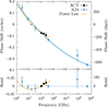 |
Fig. 4. PKS 2131–021 phase shifts measured by ACT at 95, 147, and 225 GHz (black points), compared to the phase shift results of K25 (blue points); see Table 3. We note that the ACT 95 GHz and ALMA 91.5 GHz points overlap. The Haystack or OVRO 15 GHz light curves provided the phase reference in all cases. Uncertainties were determined by the MCMC sine-wave fits (Eq. (1)). The curved blue line shows the quadratic fit determined by K25 (Eq. (3)). The orange line is the best-fit power law to the Haystack, ALMA, and ACT data (Eq. (4), Table 5). |
The best-fitting index of b = −0.3 ± 0.1 for the PKS 2131–021 mm data suggests that the jet is not optically thick in these emission zones. This may be compared to the finding in K25, based on the emission spectrum of PKS 2131–021, that the jet is optically thick below 70 GHz and optically thin above. To explore whether our result is sensitive to particular combination of frequencies, we fitted different ranges. First, since the 345 GHz point from ALMA is a notable outlier to our fit–though the goodness of fit is acceptable, with PTE = 0.07–we excluded this point and obtained  . (All fit results are shown in Table 5.) This may suggest that the jet becomes optically thinner above 225 GHz, but the difference in fits is marginal. If we restrict our fits to the phase shifts of the ACT data alone (95–225 GHz), the best-fitting index is
  , which has too broad a posterior to be informative; Fig. 5 shows that the ACT data in isolation are not sufficient to break the degeneracy of the power-law amplitude, a, and index, b. Thus, more phase-shift data are needed to probe whether the optical thickness changes through the radio, mm, and submm emission regions, but our results are most consistent with the jet being optically thin in these zones.
Figure 6 shows the frequency–phase relations from the ACT data of PKS 2131–021 and PKS J0805–0111 together with the best-fitting power laws. Interestingly, the best-fitting values for the power-law index are similar between the two AGN (0.8 and 0.7 for PKS 2131–021 and PKS J0805–0111, respectively), both of which are consistent with b = −1. However, as mentioned above, the data support a wide range of b values (see Fig. 5) so this similarity may be a coincidence.
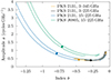 |
Fig. 5. Posterior probabilities of the power-law MC fit to the sinusoid phase shifts (Eq. (4)) for different data combinations. The contours show the 95% credible regions and the dots are the maximum likelihood values (cf. Table 5). Flat priors on a and b in the ranges of (0.05, 4) and (−2, −0.05) were used. |
In summary, two points should be noted about the phase shifts:
-
For both SMBHB candidates, the phase shift between 15 GHz and 95, 147, and 225 GHz is highly significant: χ2 for the null hypothesis of no phase shift is 548 and 1288, with three degrees of freedom, for PKS 2131–021 and PKS J0805–0111, respectively. Thus, regardless of the details of how the slope behaves in the radio and mm regime (point 2), the ACT data provide a strong detection of the phase shift between the radio and mm sinusoidal emission.
-
When all radio and mm data are considered, the power-law index is inconsistent with the jet of PKS 2131–021 being optically thick. If only the ACT data are considered, PKS 2131–021 and PKS J0805–0111 have similar best-fitting values for the power-law index, but support a wide range of values. More data are needed to understand if there is a change in jet properties in the mm zones.
Improving on these results above would not only benefit from more data, but would also require better understanding of the uncertainties of the phase shifts. As discussed in K25, intrinsic variations in the jet that are superimposed on the sinusoidal variations can add covariance between the light curves at different frequencies, complicating the noise model used in fitting. We discuss this further in Appendix C, where we also make an empirical estimate of the phase shift uncertainties by injecting sine waves into other, real ACT light curves. These uncertainties are shown with light error bars in Fig. 6. Our analysis suggests that the MCMC-derived error bars listed in Tables 1 and 2 and shown with heavy error bars in Fig. 6 are possibly underestimated. However, as we argue in Appendix C, light curves of more SMBHB candidates are needed to confirm such an assessment.
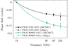 |
Fig. 6. Phase shifts of the ACT best-fit sinusoids relative to the OVRO 15 GHz light curves for each of PKS 2131–021 and PKS J0805–0111. The lines are the best fits to the power law of Eq. (4), with only ACT data included. The best-fitting values are listed in Table 5. The heavy error bars are the fiducial uncertainties of the phase shifts from the MCMC fits (Sect. 3.1) relative to 15 GHz, while the light error bars show an empirically derived, relative phase uncertainty between 95 GHz and 147–225 GHz (see Appendix C.1). Fits were done with the fiducial uncertainties. The PKS J0805–0111 points have been shifted slightly to the right for ease of viewing. |
4.2. Achromatic variability
Both the sinusoidal variation in emission (Sect. 3) and the frequency-dependent phase shifts just discussed (Sect. 4.1) provide important constraints on the physical origin of the emission and are predicted by the KO model. The model also predicts that the fractional amplitude of the sinusoidal variations should be achromatic, assuming the spectral index α is constant, since the rest-frame flux density, S′, gets boosted to S = 𝒟2 − αS′, where 𝒟 is the Doppler factor (K25). This is a third feature we verify in our data. The fractional change in intensity, expressed as  , is similar for all frequencies (see Tables 1 and 2). K25 note that it only varies by a factor of ∼2–3 over five decades in frequency, though their picture is complicated somewhat by the fact that the data were taken at several epochs. In contrast, K25 show that the OVRO and ALMA data, which were contemporaneous, show remarkably achromatic behaviour. In the OVRO + ACT data at 15, 95, 147, and 225 GHz, we find
  for PKS 2131–021, where the quoted uncertainty is the standard deviation of the ratios at the four frequencies. As with the other SMBHB properties, we once again confirm for the first time that this expected property is found in a second SMBHB candidate: PKS J0805–0111 exhibits achromaticity, with
  .
.
5. Interpreting the observations
5.1. A modified Kinetic Orbital (MKO) model
In this section we present a modified KO model, which we refer to here and in future papers as the MKO model. In the original KO model (Sobacchi et al. 2017; O22), the emitting region moves ballistically from one of the SMBH, producing a jet propagating at relativistic speeds and twisted into a conical helix by the orbital motion of the SMBH engine. The phase shift in the observed sinusoidal variations in flux between two frequencies, Δϕ, is due to the light-travel time between the two different zones of emission along the jet. Because the jet’s velocity, β = v/c, is relativistic, in the observer’s frame the jet material from the deeper zone travels almost as fast as the emitted light, such that its distance from the shallower zone, Δr, appears to be (K25)
 (5)
(5)
where γ = (1 − β)−1/2 is the Lorentz factor, c is the speed of light, PB is the binary orbital period (in the rest frame), and Δϕ is in units of cycles. For high Lorentz factors, this implies that the deeper zone has wound through multiple helical rotations before the light is emitted from the shallower zone, even though the observed phase difference is a fraction of a cycle. For instance, K25 use VLBI measurements to obtain γ = 10 for PKS 2131–021; using our best-fitting period and phase differences (Table 3), this yields a distance of ∼18 pc and ∼26 helical windings between the 15 GHz and 95 GHz emission zones. This is a potential problem with the simple KO model, because it is hard to explain how the jet can remain in a coherent helical pattern over such a distance. It would seem more likely that the phase would get smeared out.
In our new MKO model, which is described in further detail by Sullivan et al. (2025; S25 hereafter), the outflowing, ultrarelativistic jet containing the emitting electrons is not launched ballistically by its black hole source but instead follows a channel defined by a slower, mildly relativstic or sub-relativstic hydromagnetic wind that confines it. This semi-ballistic wind, possibly launched from the disc, confines the relativistic flow, dragging it around with the binary motion (Fig. 7; see also Fig. 1 in S25). The channel may only be defined for roughly 10 helical windings, but because the wind has a low Lorentz factor (cf. Eq. (5)) this suffices to account for sinusoidal variation due to the varying angle of the jet line of sight to the observer. The jet–wind complex forms a helix with pattern speed set by the wind rather than the relativistic flow. The different emission regions can thus come from a range of radii with each frequency’s minimum radius separated by less than a wavelength of the conical helix λh = βwcPB (where βw is the speed of the wind-jet boundary and sets the pattern speed) and the average radius need not be separated by more than ∼10 λh. S25 show that plausible parameters in the MKO model are able to reproduce the amplitudes and phase shifts of the multi-wavelength light curves for both PKS 2131–021 and PKS J0805–0111 (see Figs. 5 and 6 in S25). With these parameters, the separation between the 15 GHz and 345 GHz emission zones is ∼10 helical windings (see Fig. 4 in S25), consistent with the desideratum that the jet confinement not be excessively long.
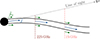 |
Fig. 7. A 2D slice through the wind-collimated jet, illustrating the MKO model. The relativistic flow velocity, β, at a particular point in the jet is parallel to the local wind velocity, βw. The wind propagates semi-ballistically, so different distances along the jet have local wind velocity directions out of phase. Since it is the aberration caused by the changing jet velocity that modulates the observed flux, frequencies originating from different locations in the jet that are observed simultaneously are at different phases in their sinusoidal flux variations. |
Our analysis of the sinusoid phase shifts in Sect. 4.1 shows that the ACT data alone cannot constrain the power law Δϕ ∝ νb well, but that when Haystack and ALMA data are included, there is evidence of b < 1 for PKS 2131–021. This differs from the classic scaling expected for the depth of a marginally optically thick photosphere as a function of frequency r ∝ ν−1 (Blandford & Königl 1979) and would suggest that the emission does not come entirely from an optically thick photosphere as in the classic simple picture but instead arises from both optically thin and optically thick regions. If optically thin, the observed emission at each radius would also contain the tail of the local synchrotron spectrum (S25), and the frequency of the emissivity cut-off would thus decrease with distance along the jet, as can be seen in Fig. 4 of S25.
5.2. Simulations that address the intermittency of the periodicity
An observed feature of both PKS 2131–021 and PKS J0805–0111 that is not explained by the MKO model as presented thus far is the intermittency of the sinusoid pattern (see Sect. 3.3). Here, we provide for the first time a possible physical explanation for this phenomenon. It is based upon the possibility of precession or disturbances in the SMBH accretion disc temporarily disrupting the production of a jet. Synchrotron emission from much further out in the jet is responsible for the baseline synchrotron emission (as found by O22 via VLBI measurements of PKS 2131–021), while the sinusoidal component is produced by the MKO mechanism near the central engine. When the jet is disrupted at its base, the sinusoidal signal shuts off, but when the jet relaunches the new sinusoid is in phase with the previous sinusoid because the SMBHB orbit has continued unabated.
This picture is supported by recent numerical simulations which have have extensively investigated black hole accretion flows (see e.g. Davis & Tchekhovskoy 2020 for a recent review). Three-dimensional simulations of magnetised circumbinary accretion, in particular on black hole binaries, have also advanced considerably (Farris et al. 2012; Gold et al. 2014; Manikantan et al. 2025; Ennoggi et al. 2025; Avara et al. 2024). In the context of circumbinary disc formation from intermediate galactic scale accretion, Wang et al. (2025) have recently shown that realistic circumbinary discs might be strongly warped and tilted (Nixon et al. 2013; see also Guo et al. 2025 for a similar study on single black holes). Although these simulations focus on equal-mass black hole binaries, the disc tilt originates from large-scale inflow and is expected to persist in systems with unequal mass ratios. These tilted accretion discs launch jets along the disc’s rotation axis rather than the black hole’s, as shown by Liska et al. (2018), who employed 3D general relativistic magnetohydrodynamic simulations. Liska et al. (2018) show how strong magnetic flux can partially realign the inner disc and jets with the black hole spin. On longer timescales, the entire disc-jet system undergoes Lense-Thirring precession (Lense & Thirring 1918). This precession can produce curved jet morphologies and, in some cases, disrupt the accretion flow and shut off the jets. Misaligned circumbinary accretion discs around a binary black hole system lead to disc tearing, caused by strong differential torques (Nixon et al. 2013; Kaaz et al. 2025), which can result in jets shutting off. As such, realistic accretion environments might naturally be able to explain the temporary absence of a jet, with the timescale potentially being correlated with the inner disc precession timescale.
Even in the absence of disc tilt and precession, the accretion flow onto one constituent black hole in the binary can naturally feature variability. Lalakos et al. (2025) show that extremely long-duration 3D general relativistic magnetohydrodynamic Bondi-like simulations (see also Cho et al. 2023; Galishnikova et al. 2025; Guo et al. 2025) can exhibit transitions between a magnetically arrested disc (MAD) state (Narayan et al. 2003; Tchekhovskoy et al. 2011), characterised by strong, stable jets, and a rocking accretion disc (RAD; Lalakos et al. 2024). In the RAD state, the gas angular momentum is randomly oriented and chaotic, which leads to violently precessing inner accretion discs. The RAD jets are weaker as they tilt, wobble, and dissipate within a few thousand gravitational radii. These simulations show that MAD-to-RAD cycles occur on timescales of τ ∼ 105 rg c−1, where rg is the black hole’s gravitational radius. For a 108 M⊙ black hole, τ ∼ 600 days–comparable to the orbital period of our SMBHB candidates. In this scenario, continued monitoring of such systems may reveal multiple accretion and jet activity cycles tied to the Bondi accretion timescale of the individual black hole rather than the binary’s orbital period.
6. The value of millimetre light curves for SMBHB searches
A notable feature of the mm light curves shown in Figs. 1 and 3 is their short-term deviations from the sinusoids. However, for the 95 and 147 GHz light curves, the sinusoidal variation dominates by a factor of ∼2–3.5 (see the S/Nsin values in Table C.1). Thus, although the mm light curves do not have the same sensitivity as the OVRO 15 GHz light curves, and hence the uncertainties on individual observations are much larger in the ACT than in the OVRO data, this does not mean that ACT is less sensitive to sinusoidal light curves in blazars than the OVRO, provided we consider equal timespans11. This argues strongly for continued, long-term observations with mm survey instruments, such as the South Pole Telescope (Carlstrom et al. 2011; Benson et al. 2014), the Simons Observatory (SO; Ade et al. 2019; Abitbol et al. 2025) and the CCAT Observatory (CCAT-Prime Collaboration 2023) for multi-messenger astronomy.
The promise of centimetre (cm), mm, and submm data for identifying and studying SMBHB is evident when they are placed side by side with optical data. Figure 8 shows the OVRO 15 GHz light curve of PKS 2131–021 together with optical light curves of the same object from CRTS and ZTF. As discussed in K25, the ZTF data show much stronger short-term variations than the radio–submm data, but when averaged over a year they follow a sine wave well and have a period consistent with that derived from the OVRO and Haystack 15 GHz observations. To further explore this point, in Appendix D we give a detailed account of statistical tests we carried out on the CRTS and ZTF data for PKS 2131–021 and show that the optical data alone do not provide compelling evidence for the periodicity we see in PKS 2131–021, unless they are sampled about 3 times a week and then averaged for a long period (∼several months) to eliminate the rapid large fluctuations at optical wavelengths. This is illustrated in Fig. 8 by the sine wave, fitted to ZTF data by K25 (reported in their Table 4), and here extrapolated back to the period covered by the CRTS. There is no clear correspondence between the curve and the CRTS data points, suggesting that searches for SMBHB candidates similar to PKS 2131–021 are unlikely to be found in the CRTS because the cadence is not frequent enough. The ZTF cadence is two days, and that clearly works well, although the short-term variations are much greater than at cm, mm, and submm wavelengths. We do not offer any specific theories here about the origin of this behaviour, but it is reasonable to suppose that activity near the central engine could produce very different short-term variations than those seen from the more distant zones producing the radio and mm radiation.
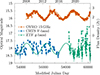 |
Fig. 8. Comparison of radio and optical light curves of PKS 2131–021. The sine waves shown in the figure come from Tables 1 and 4 of K25 for the radio and ZTF optical data, respectively. The fit to the ZTF data has been extrapolated back in time to show that the cadence of the CRTS is not sufficient to easily discover this sinusoidal pattern (see text for additional details). |
Ren et al. (2025) also find only weak evidence for periodicity from a Lomb-Scargle analysis of infrared (WISE and NEOWISE) and optical (ZTF, CRTS, and Asteroid Terrestrial-impact Last Alert System) light curves of PKS 2131–021, further highlighting the importance of cm, mm, and submm data for this class of SMBHB candidate.
The cm, mm, and submm observations also have the great advantage that they can be sampled year-round, while at optical frequencies the daylight sky is bright compared to even the brightest optical blazar, 3C 273, which has an apparent optical magnitude of V ∼ 1312, so year-round optical monitoring of blazars is not possible13. Nevertheless, there is evidence for SMBHB candidates that show more prominent sinusoidal variations at optical wavelengths. PG 1302−102 might be just such an example (Graham et al. 2015): this source also shows radio periodicity at the same period as detected in the optical (Qian et al. 2018). Recently, Huijse et al. (2025) reported the detection of 181 SMBHB candidates from a search of 770 100 AGN that were monitored for 34 months in the optical by the Gaia satellite. It is therefore likely that optical and cm, mm, and submm observations will be highly synergistic for discovering and characterising SMBHBs.
7. Summary and discussion
ACT millimetre data at 95, 147, and 225 GHz have confirmed the presence of a sinusoidal variation in the light curves of PKS 2131–021 and PKS J0805–0111 that had been detected with high significance in OVRO 15 GHz data by O22, D25, and K25. Our main findings are as follows:
-
The ACT 95 GHz light curve of PKS 2131–021 is in good agreement with the ALMA 91.5 and 103.5 GHz light curves, including in their small variations superimposed on the larger sinusoid variation. This confirms that the ACT calibration and data reduction of light curves are working well.
-
ACT light curves of PKS J0805–0111, for which no ALMA data are available, corroborate the finding in D25 that this source is a SMBHB candidate. Especially compelling is the fact that the sinusoid appears to turn off in the ACT light curves in the same manner as in the OVRO data in mid-2020 (see Fig. 3). This provides further evidence that (a) the long timescale variations of the mm light curves are tracing the same underlying physics as the radio light curve and (b) that the phenomenon of the sinusoid stopping and starting, discovered in O22 for PKS 2131–021, is likely a common feature of SMBHB candidates. It can be explained as the temporary disruption of the jet by precession or by MAD-to-RAD transitions of the accretion disc. Further data will help clarify these hypotheses, and our results show that mm observations can play a key role in detecting this behaviour.
-
The ACT data confirm that the sinusoidal variations at higher frequencies are shifted in phase relative to radio frequencies, a feature that is naturally explained in the MKO model by light-travel times due to higher frequencies originating from deeper in the jet. In both cases the mm phase leads the radio phase in time.
-
A power-law fit to the phase shifts in PKS 2131–021 in the radio to submm regime suggests that the jet in these emission zones is optically thin, but it is unclear whether the jet properties are uniform throughout the regions. ACT data alone cannot constrain the power-law index well for either PKS J0805–0111 or PKS 2131–021 given the current uncertainties.
-
The sinusoidal signal is achromatic from 15 to 225 GHz, i.e. the ratio of its amplitude to offset,
 , is nearly constant at all measured frequencies in this range. This is expected under the MKO model and is further evidence for these objects being SMBHBs.
 -
In PKS 2131–021, the ratio of the sinusoid amplitude to the non-sinusoidal variations in the mm data is significantly higher than in optical data, which are contaminated by large short-term variability from the point of view of detecting SMBHB candidates. It seems likely that some SMBHB candidates will appear more cleanly in the optical (e.g. PG 1302−102, Graham et al. 2015; see also Huijse et al. 2025), but our findings provide strong motivation for using mm surveys to search for SMBHBs. Such searches will be complementary to radio, submm, and optical searches.
In addition to these empirical findings, we have presented the MKO model which, when combined with recent findings from simulated BH accretion discs, explains all four of the properties observed in the two SMBHB candidates: (a) the flux density exhibits a sinusoidal pattern; (b) the sinusoid is monochromatic, in that it has the same period and a similar amplitude to mean-flux ratio over a broad range of frequencies; (c) the phase of the sinusoid shifts monotonically with frequency; (d) the sinusoidal variations are intermittent on timescales ≳ the SMBHB period.
Our results demonstrate the value of high cadence, wide area surveys of the mm and submm sky available from CMB and mm/submm survey experiments such as SPT, SO, and CCAT. In particular, the large aperture telescope (LAT) of SO will observe 25 000 deg2 of the sky from 2025 to 2034 at 27, 39, 93, 145, 225, and 280 GHz with a planned cadence of 1–2 days (Abitbol et al. 2025)14. We used their goal sensitivity for single observations at 93 GHz to forecast the number of AGN that SO can monitor over a 21 000 deg2 sky area (to exclude the Galactic plane), using the 90 GHz radio number counts of Lagache et al. (2020). We find that SO will be able to monitor ∼8000 AGN with a signal-to-noise ratio > 5, if we allow six measurements to be binned together (i.e. corresponding to a 1–2 week cadence). The number will increase to ∼12 000 when the Advanced SO upgrades, which will double the number of detectors, are completed by 2028. Estimating the rates of blazars in SMBHBs depends on a number of factors, as discussed in K25 and D25, but these authors conclude that with current information, ∼1 in 100 blazars may be in SMBHB systems. If this is correct then SO should be able to observe 𝒪(100) SMBHB candidates. This large sample size will better constrain the SMBHB occurrence rate. At this point PKS 2131–021 is the only blazar in which sinusoidal variations have been observed at both optical and radio wavelengths15, but this is unlikely to be an isolated case given the broad-band sinusoidal variations of PKS J0805–0111 that we present in this paper, making a compelling case for joint searches for SMBHB candidates spanning from the radio to optical.
The nature of sinusoidal blazar signals and their potential connection with supermassive black hole binaries is of fundamental interest for both astrophysics and cosmology. Multi-wavelength information about more systems and over more periods, as will be possible with upcoming mm wave surveys, will establish the correct model of emission and its connection to binary properties, including the duty cycle for sinusoidal emission and the selection function for observing binaries. Significant detections of correlated gravitational wave and electromagnetic signals from particular SMBHB systems are also imminent (Agarwal et al. 2025). In principle, the absolute phase of mm-discovered SMBHBs could be obtained from optical light curves, since the optical emission is believed to originate close to the AGN core and would therefore be virtually in phase with the SMBHB orbit. Further, if velocities were obtained from optical spectra, the masses could be derived, and the expected gravitational wave phase and amplitude of each source could be determined. One could then mount coherent gravitational wave searches with millisecond pulsar timing arrays, rather than searching within the stochastic noise, potentially expanding their reach to weaker sources of gravitational waves. In turn, these observations and binary blazar models could provide more reliable observation-based estimates of the total binary population with orbital periods of years. This population is of intense interest for its production of gravitational waves: the Laser Interferometer Space Antenna (LISA) will directly measure the supermassive binary merger rate throughout the Hubble volume, and comparison with the total years-period binary population will constrain the complex galactic dynamics and astrophysical mechanisms driving binary mergers (e.g. Antonini et al. 2015; Nasim et al. 2020; Milosavljević & Merritt 2003).
In addition, the close-orbit SMBHB population will likely provide a dominant contribution to the stochastic background of gravitational waves at nanohertz frequencies for pulsar timing arrays or astrometric probes (Agazie et al. 2023c). This stochastic background complicates the prospects for detecting other cosmological sources of gravitational waves from the early universe (Boileau et al. 2021), such as phase transitions or reheating after inflation (see Afzal et al. 2023 for a recent overview). A detailed understanding of the SMBHB population enabled by multi-wavelength blazar observations may eventually be key to exploiting unique gravitational wave information about physics at the highest energy scales.
References
- Abitbol, M., Abril-Cabezas, I., Adachi, S., et al. 2025, JCAP, 2025, 034 [Google Scholar]
- Ade, P., Aguirre, J., Ahmed, Z., et al. 2019, JCAP, 2019, 056 [Google Scholar]
- Afzal, A., Agazie, G., Anumarlapudi, A., et al. 2023, ApJ, 951, L11 [NASA ADS] [CrossRef] [Google Scholar]
- Agarwal, N., Agazie, G., Anumarlapudi, A., et al. 2025, ApJL, accepted [arXiv:2508.16534] [Google Scholar]
- Agazie, G., Anumarlapudi, A., Archibald, A. M., et al. 2023a, ApJ, 951, L8 [NASA ADS] [CrossRef] [Google Scholar]
- Agazie, G., Anumarlapudi, A., Archibald, A. M., et al. 2023b, ApJ, 951, L50 [NASA ADS] [CrossRef] [Google Scholar]
- Agazie, G., Anumarlapudi, A., Archibald, A. M., et al. 2023c, ApJ, 952, L37 [NASA ADS] [CrossRef] [Google Scholar]
- An, T., Baan, W. A., Wang, J.-Y., Wang, Y., & Hong, X.-Y. 2013, MNRAS, 434, 3487 [Google Scholar]
- Antonini, F., Barausse, E., & Silk, J. 2015, ApJ, 812, 72 [Google Scholar]
- Astropy Collaboration. 2013, A&A, 558, A33 [NASA ADS] [CrossRef] [EDP Sciences] [Google Scholar]
- Astropy Collaboration. 2018, AJ, 156, 123 [Google Scholar]
- Astropy Collaboration. 2022, ApJ, 935, 167 [NASA ADS] [CrossRef] [Google Scholar]
- Avara, M. J., Krolik, J. H., Campanelli, M., et al. 2024, Astrophys. J., 974, 242 [Google Scholar]
- Backer, D. C., Kulkarni, S. R., Heiles, C., Davis, M. M., & Goss, W. M. 1982, Nature, 300, 615 [NASA ADS] [CrossRef] [Google Scholar]
- Benson, B. A., Ade, P. A. R., Ahmed, Z., et al. 2014, SPIE Conf. Ser., 9153, 91531P [NASA ADS] [Google Scholar]
- Blandford, R. D., & Königl, A. 1979, ApJ, 232, 34 [Google Scholar]
- Blandford, R., Meier, D., & Readhead, A. 2019, ARA&A, 57, 467 [NASA ADS] [CrossRef] [Google Scholar]
- Boileau, G., Christensen, N., Meyer, R., & Cornish, N. J. 2021, Phys. Rev. D, 103, 103529 [Google Scholar]
- Braginsky, V. B., Kardashev, N. S., Polnarev, A. G., & Novikov, I. D. 1990, Nuovo Cimento B Ser., 105, 1141 [Google Scholar]
- Carlstrom, J. E., Ade, P. A. R., Aird, K. A., et al. 2011, PASP, 123, 568 [CrossRef] [Google Scholar]
- CCAT-Prime Collaboration (Aravena, M., et al.) 2023, ApJS, 264, 7 [NASA ADS] [CrossRef] [Google Scholar]
- Cho, H., Prather, B. S., Narayan, R., et al. 2023, ApJ, 959, L22 [Google Scholar]
- Choi, S. K., Hasselfield, M., Ho, S.-P. P., et al. 2020, JCAP, 2020, 045 [CrossRef] [Google Scholar]
- Coulton, W., Madhavacheril, M. S., Duivenvoorden, A. J., et al. 2024, Phys. Rev. D, 109, 063530 [NASA ADS] [CrossRef] [Google Scholar]
- Davis, S. W., & Tchekhovskoy, A. 2020, Ann. Rev. Astron. Astrophys., 58, 407 [Google Scholar]
- de la Parra, P. V., Kiehlmann, S., Mróz, P., et al. 2025, ApJ, 987, 191 [Google Scholar]
- Drake, A. J., Djorgovski, S. G., Mahabal, A., et al. 2009, ApJ, 696, 870 [Google Scholar]
- Drinkwater, M. J., Webster, R. L., Francis, P. J., et al. 1997, MNRAS, 284, 85 [NASA ADS] [Google Scholar]
- Emmanoulopoulos, D., McHardy, I. M., & Papadakis, I. E. 2013, MNRAS, 433, 907 [NASA ADS] [CrossRef] [Google Scholar]
- Ennoggi, L., Campanelli, M., Zlochower, Y., et al. 2025, Phys. Rev. D, 112, 063009 [Google Scholar]
- EPTA Collaboration. 2023, A&A, 678, A50 [CrossRef] [EDP Sciences] [Google Scholar]
- Farren, G. S., Partridge, B., Kneissl, R., et al. 2021, ApJS, 256, 19 [NASA ADS] [CrossRef] [Google Scholar]
- Farris, B. D., Gold, R., Paschalidis, V., Etienne, Z. B., & Shapiro, S. L. 2012, Phys. Rev. Lett., 109, 221102 [Google Scholar]
- Foreman-Mackey, D., Hogg, D. W., Lang, D., & Goodman, J. 2013, PASP, 125, 306 [Google Scholar]
- Galishnikova, A., Philippov, A., Quataert, E., Chatterjee, K., & Liska, M. 2025, Astrophys. J., 978, 148 [Google Scholar]
- Gold, R., Paschalidis, V., Etienne, Z. B., Shapiro, S. L., & Pfeiffer, H. P. 2014, Phys. Rev. D, 89, 064060 [NASA ADS] [CrossRef] [Google Scholar]
- Graham, M. J., Djorgovski, S. G., Stern, D., et al. 2015, Nature, 518, 74 [Google Scholar]
- Graham, M. J., Kulkarni, S. R., Bellm, E. C., et al. 2019, PASP, 131, 078001 [Google Scholar]
- Guo, M., Stone, J. M., Quataert, E., & Springel, V. 2025, ApJ, 987, 202 [Google Scholar]
- Harris, C. R., Millman, K. J., van der Walt, S. J., et al. 2020, Nature, 585, 357 [NASA ADS] [CrossRef] [Google Scholar]
- Henderson, S. W., Allison, R., Austermann, J., et al. 2016, J. Low Temp. Phys., 184, 772 [NASA ADS] [CrossRef] [Google Scholar]
- Hervías-Caimapo, C., Naess, S., Hincks, A. D., et al. 2024, MNRAS, 529, 3020 [Google Scholar]
- Huijse, P., Davelaar, J., De Ridder, J., Jannsen, N., & Aerts, C. 2025, ArXiv e-prints [arXiv:2505.16884] [Google Scholar]
- Ingram, A. R., & Motta, S. E. 2019, New Astron. Rev., 85, 101524 [Google Scholar]
- Kaaz, N., Lithwick, Y., Liska, M., & Tchekhovskoy, A. 2025, ApJ, 979, 192 [Google Scholar]
- Kiehlmann, S. 2023, Astrophysics Source Code Library [record ascl:2310.002] [Google Scholar]
- Kiehlmann, S., de la Parra, P. V., Sullivan, A. G., et al. 2025, ApJ, 985, 59 [Google Scholar]
- Krolik, J. H., & Di Matteo, T. 2000, Am. J. Phys., 68, 489 [Google Scholar]
- Lagache, G., Béthermin, M., Montier, L., Serra, P., & Tucci, M. 2020, A&A, 642, A232 [NASA ADS] [CrossRef] [EDP Sciences] [Google Scholar]
- Lalakos, A., Tchekhovskoy, A., Bromberg, O., et al. 2024, ApJ, 964, 79 [NASA ADS] [CrossRef] [Google Scholar]
- Lalakos, A., Tchekhovskoy, A., Most, E. R., et al. 2025, ArXiv e-prints [arXiv:2505.23888] [Google Scholar]
- Lense, J., & Thirring, H. 1918, Phys. Z., 19, 156 [Google Scholar]
- Liska, M., Hesp, C., Tchekhovskoy, A., et al. 2018, MNRAS, 474, L81 [Google Scholar]
- Lomb, N. R. 1976, Ap&SS, 39, 447 [Google Scholar]
- Madhavacheril, M. S., Hill, J. C., Næss, S., et al. 2020, Phys. Rev. D, 102, 023534 [Google Scholar]
- Manikantan, V., Paschalidis, V., & Bozzola, G. 2025, ApJ, 984, L47 [Google Scholar]
- Marriage, T. A., Baptiste Juin, J., Lin, Y.-T., et al. 2011, ApJ, 731, 100 [Google Scholar]
- Masci, F. J., Laher, R. R., Rusholme, B., et al. 2019, PASP, 131, 018003 [Google Scholar]
- Max-Moerbeck, W., Richards, J. L., Hovatta, T., et al. 2014, MNRAS, 445, 437 [NASA ADS] [CrossRef] [Google Scholar]
- Miles, M. T., Shannon, R. M., Reardon, D. J., et al. 2025, MNRAS, 536, 1489 [Google Scholar]
- Milosavljević, M., & Merritt, D. 2003, ApJ, 596, 860 [Google Scholar]
- Molina, B., Mróz, P., De la Parra, P. V., et al. 2025, ArXiv e-prints [arXiv:2510.23103] [Google Scholar]
- Moore, C. J., Mihaylov, D. P., Lasenby, A., & Gilmore, G. 2017, Phys. Rev. Lett., 119, 261102 [Google Scholar]
- Naess, S., Guan, Y., Duivenvoorden, A. J., et al. 2025, JCAP, 2025, 061 [Google Scholar]
- Narayan, R., Igumenshchev, I. V., & Abramowicz, M. A. 2003, PASJ, 55, L69 [NASA ADS] [Google Scholar]
- Nasim, I., Gualandris, A., Read, J., et al. 2020, MNRAS, 497, 739 [Google Scholar]
- Niemack, M. D. 2008, Ph.D. Thesis, Princeton University, New Jersey [Google Scholar]
- Nixon, C., King, A., & Price, D. 2013, MNRAS, 434, 1946 [NASA ADS] [CrossRef] [Google Scholar]
- O’Brien, T. A., Collins, W. D., Rauscher, S. A., & Ringler, T. D. 2014, Comp. Stats. & Data Anal., 79, 222 [Google Scholar]
- O’Brien, T. A., Kashinath, K., Cavanaugh, N. R., Collins, W. D., & O’Brien, J. P. 2016, Comp. Stats. & Data Anal., 101, 148 [Google Scholar]
- O’Neill, S., Kiehlmann, S., Readhead, A. C. S., et al. 2022, ApJ, 926, L35 [CrossRef] [Google Scholar]
- Paliya, V. S., Marcotulli, L., Ajello, M., et al. 2017, ApJ, 851, 33 [NASA ADS] [CrossRef] [Google Scholar]
- Qian, S. J., Britzen, S., Witzel, A., Krichbaum, T. P., & Kun, E. 2018, A&A, 615, A123 [NASA ADS] [CrossRef] [EDP Sciences] [Google Scholar]
- Readhead, A. C. S. 1980, in Objects of High Redshift, eds. G. O. Abell, & P. J. E. Peebles, 92, 165 [Google Scholar]
- Readhead, A. C. S. 2024, J. Astron. Hist. Heritage, 27, 453 [Google Scholar]
- Readhead, A. C. S., & Hewish, A. 1974, MmRAS, 78, 1 [Google Scholar]
- Readhead, A. C. S., Cohen, M. H., Pearson, T. J., & Wilkinson, P. N. 1978, Nature, 276, 768 [Google Scholar]
- Readhead, A. C. S., Aller, M. F., Sullivan, A. G., et al. 2025, ArXiv e-prints [arXiv:2511.09409] [Google Scholar]
- Ren, G.-W., Ding, N., Zhang, X., et al. 2021a, MNRAS, 506, 3791 [CrossRef] [Google Scholar]
- Ren, G.-W., Zhang, H.-J., Zhang, X., et al. 2021b, Res. Astron. Astrophys., 21, 075 [Google Scholar]
- Ren, G.-W., Sun, M., Ding, N., Yang, X., & Zhang, Z.-X. 2025, MNRAS, 537, 2931 [Google Scholar]
- Richards, J. L., Max-Moerbeck, W., Pavlidou, V., et al. 2011, ApJS, 194, 29 [Google Scholar]
- Scargle, J. D. 1982, ApJ, 263, 835 [Google Scholar]
- Sobacchi, E., Sormani, M. C., & Stamerra, A. 2017, MNRAS, 465, 161 [NASA ADS] [CrossRef] [Google Scholar]
- Sullivan, A. G., Blandford, R. D., Synani, A., et al. 2025, ApJ, accepted [arXiv:2510.02301] [Google Scholar]
- Swetz, D. S., Ade, P. A. R., Amiri, M., et al. 2011, ApJS, 194, 41 [NASA ADS] [CrossRef] [Google Scholar]
- Tchekhovskoy, A., Narayan, R., & McKinney, J. C. 2011, MNRAS, 418, L79 [NASA ADS] [CrossRef] [Google Scholar]
- Thornton, R. J., Ade, P. A. R., Aiola, S., et al. 2016, ApJS, 227, 21 [Google Scholar]
- Virtanen, P., Gommers, R., Oliphant, T. E., et al. 2020, Nat. Methods, 17, 261 [Google Scholar]
- Wang, J.-Y., An, T., Baan, W. A., & Lu, X.-L. 2014, MNRAS, 443, 58 [Google Scholar]
- Wang, H.-Y., Guo, M., Most, E. R., Hopkins, P. F., & Lalakos, A. 2025, ArXiv e-prints [arXiv:2504.03874] [Google Scholar]
- Zechmeister, M., & Kürster, M. 2009, A&A, 496, 577 [CrossRef] [EDP Sciences] [Google Scholar]
There were two crucial steps in the discovery of millisecond pulsars: (i) the discovery of interplanetary scintillation, at Galactic latitude −0.3°, in 4C 21.53 by Readhead & Hewish (1974, see Readhead 2024) which drew attention to the singular nature of this object; and (ii) the discovery of millisecond pulses from 4C 21.53W by Backer et al. (1982).
In the latter part of the review process of our paper, two preprints reporting a third candidate SMBHB found in OVRO and University of Michigan Radio Astronomy Observatory data, PKS 1309+1154, were posted to the arXiv (Molina et al. 2025; Readhead et al. 2025).
For f150 we have given the mean excluding PA1, since that array was removed before the light curves in this paper begin. With PA1 included the mean band centre of f150 is 146.9 GHz.
The 147 GHz data from PA4 lack the final, Planck-based correction due to issues with the ACT power spectra for these data (Naess et al. 2025). Since these corrections for other frequency-arrays are of the order of a few percent, comparable to our uncertainty (see below), this should not noticeably affect our results in this paper.
For details, see the documentation for the matched_filter_constcorr_dual() method in the pixell package: https://github.com/simonsobs/pixell
This AGN is well known in the literature as PKS J2134−0153, but we use the identifier PKS 2131–021 to be in continuity with O22 and K25.
In principle, the ACT band centre should also be colour-corrected, since we have adopted the band centre for synchrotron emission, i.e. an index of −0.7 (see Sect. 2.1). However, the difference is subdominant to other uncertainties, particularly the ≈3% scatter in band centre from detector array to detector array, and we ignored it in this analysis.
We have converted the values they report, which are in units of days, to units of cycles using their radio period of 1760 ± 33 days.
Including the infrared and optical frequencies result in a poor fit, so we omit them. This is not necessarily surprising: the emission is likely to be more complicated at these higher frequencies, which originate close to the central engine, thus affecting the scaling of the phase shifts.
The 225 GHz channel has more noise due to the larger atmospheric contamination it suffers, and also has lower fluxes due to the falling synchrotron spectrum. It will therefore not be as important a channel for SMBHB detection. Nonetheless, for our SMBHB candidates, its S/N of ≈1 (Table C.2), will still allow 225 GHz data to be used to study phase shifts and spectra.
See the NASA/IPAC Extragalactic Database (NED).
While AGN can be observed in daylight in the mm, it is still the case that mid-latitude CMB surveys will have observing gaps for most AGN for part of the year–about one month for SO–due to Sun- and Moon-avoidance in their observation strategies (Abitbol et al. 2025).
Though see footnote 13.
The report of 181 SMBHB candidates found in optical Gaia data by Huijse et al. (w2025; see Sect. 6) was posted to the arXiv while this paper was in review; we have not yet followed up these candidates in our data.
The MAD is the distance between the 50th and 75th percentiles (assuming the distribution is symmetric), which for a Gaussian is equal to 
The 95–225 GHz result for PKS 2131–021 is the noisiest, with the uncertainty estimate varying by a factor of 2.5 for shifts between −2% and 2%.
We used this Python package for the power spectral density analysis: https://github.com/skiehl/psd_analysis.
Appendix A: Acknowledgements
We thank the two anonymous referees for comments that strengthened our analysis and prompted us to introduce the MKO model.
This work was supported by the U.S. National Science Foundation through awards AST-0408698, AST-0965625, and AST-1440226 for the ACT project, as well as awards PHY-0355328, PHY-0855887, and PHY-1214379. Funding was also provided by Princeton University, the University of Pennsylvania, and a Canada Foundation for Innovation (CFI) award to UBC.
ACT operated in the Parque Astronómico Atacama in northern Chile under the auspices of the Agencia Nacional de Investigación y Desarrollo (ANID; formerly Comisión Nacional de Investigación Científica y Tecnológica de Chile, or CONICYT). We thank the Republic of Chile for hosting ACT in the northern Atacama, and the local indigenous Licanantay communities whom we follow in observing and learning from the night sky.
The development of multichroic detectors and lenses for ACT was supported by NASA grants NNX13AE56G and NNX14AB58G. Detector research at NIST was supported by the NIST Innovations in Measurement Science program. Computing for ACT was performed using the Princeton Research Computing resources at Princeton University, the National Energy Research Scientific Computing Center (NERSC), and the Niagara supercomputer at the SciNet HPC Consortium. SciNet is funded by Innovation, Science and Economic Development Canada; the Digital Research Alliance of Canada; the Ontario Research Fund: Research Excellence; and the University of Toronto. It has also previously been funded by the Canada Foundation for Innovation.
Colleagues at AstroNorte and RadioSky provided logistical support for ACT and kept operations in Chile running smoothly. We also thank the Mishrahi Fund and the Wilkinson Fund for their generous support of the project.
The OVRO programme was supported by NASA grants NNG06GG1G, NNX08AW31G, NNX11A043G, and NNX13AQ89G from 2006 to 2016 and NSF grants AST-0808050 and AST-1109911 from 2008 to 2014. This work is currently supported by NSF grants AST2407603 and AST2407604.
This is not an official SO Collaboration paper.
ADH acknowledges support from the Sutton Family Chair in Science, Christianity and Cultures, from the Faculty of Arts and Science, University of Toronto, and from the Natural Sciences and Engineering Research Council of Canada (NSERC) [RGPIN-2023-05014, DGECR-2023-00180], and is further grateful to the Lumen Christi Institute for support that enabled a research visit to the University of Chicago, during which significant portions of this work were done. S.K. was funded by the European Union ERC-2022-STG – BOOTES – 101076343. Views and opinions expressed are however those of the author(s) only and do not necessarily reflect those of the European Union or the European Research Council Executive Agency. Neither the European Union nor the granting authority can be held responsible for them. CS acknowledges support from the Agencia Nacional de Investigación y Desarrollo (ANID) through Basal project FB210003. MJG acknowledges support from NSF grant AST-2108402.
This paper makes use of the following ALMA data: ADS/JAO.ALMA#2011.0.00001.CAL. ALMA is a partnership of ESO (representing its member states), NSF (USA) and NINS (Japan), together with NRC (Canada), NSTC and ASIAA (Taiwan), and KASI (Republic of Korea), in cooperation with the Republic of Chile. The Joint ALMA Observatory is operated by ESO, AUI/NRAO and NAOJ. The National Radio Astronomy Observatory is a facility of the National Science Foundation operated under cooperative agreement by Associated Universities, Inc.
The CSS survey is funded by the National Aeronautics and Space Administration under Grant No. NNG05GF22G issued through the Science Mission Directorate Near-Earth Objects Observations Program. The CRTS survey is supported by the U.S. National Science Foundation under grants AST-0909182 and AST-1313422.
ZTF is supported by the NSF under Grants No. AST-1440341 and AST-2034437 and a collaboration including current partners Caltech, IPAC, the Oskar Klein Center at Stockholm University, the University of Maryland, University of California, Berkeley, the University of Wisconsin at Milwaukee, University of Warwick, Ruhr University, Cornell University, Northwestern University and Drexel University. Operations are conducted by COO, IPAC, and UW.
This research has made use of the NASA/IPAC Extragalactic Database (NED), which is funded by the National Aeronautics and Space Administration and operated by the California Institute of Technology.
Some of the results/plots in this paper have been derived/produced using the following software: ASTROPY16, a community-developed core Python package for Astronomy (Astropy Collaboration 2013, 2018, 2022); EMCEE (Foreman-Mackey et al. 2013); FASTKDE (O’Brien et al. 2014; O’Brien et al. 2016); GNUPLOT17; NUMPY (Harris et al. 2020); PIXELL18; and SCIPY (Virtanen et al. 2020).
Appendix B: ALMA sine-wave fit results
K25 performed sine-wave fits to the OVRO and ALMA data for PKS 2131–021 using the same methodology described in Sect. 3.1, but only report the best-fitting phase shifts. For completeness we include all the best-fitting parameters from this analysis in Table B.1.
Sine-wave fit results for PKS 2131–021.
Appendix C: Empirical estimates of phase shift uncertainties
C.1. Background
Given the important information about SMBHB jet physics encoded in the phase of the sinusoidal variation of the light curves as a function of frequency, it is important to assess how well we can measure those phase shifts. There are at least two types of uncertainty associated with them. The absolute error encodes how uncertain the phase measurement of a light curve is with respect to the true, underlying sinusoid. The relative error encodes how uncertain the phase shifts at two different frequencies are with respect to each other, rather than to the true, underlying sinusoid. This is the more relevant uncertainty for probing how the location of the emission zone in the jet varies with frequency. If the light curves consisted of a pure sine wave with white noise, then the absolute and relative errors would be identical. In reality, the noise is correlated within single light curves and between light curves of different frequencies, and so the two types of uncertainty will be different.
Some background on physical origin of the light curves is in order. The radio flux density variations in blazars originate from a number of sites along the jet, but are dominated by the variations in the core, which is unresolved even by VLBI (Blandford et al. 2019). These variations in blazars are believed to generally follow a power-law spectrum (see e.g. Max-Moerbeck et al. 2014), so it is to be expected that there will be ongoing, non-sinusoidal variations on both longer and shorter timescales than the sinusoidal variations. When a limited number of sinusoid cycles is measured, the superimposed variations can bias the phase shift. This is evident, for instance, in the 15 GHz OVRO light curve of PKS 2131–021 in Fig. 1. One can see by eye that if the dashed orange curve, representing the best-fit sine wave to the OVRO data during the period when ALMA data are available, were continued half a cycle to the left, such that it extended into ∼2010–2014, it would not line up perfectly with the data points due to superimposed variations during this time range. Another feature to note in this plot is the fluctuation of the ALMA and ACT data points above the sine curve in the year 2018: one sees the same trend at all the mm frequencies (Fig. 2), which also appears to be present in the 15 GHz OVRO data earlier, at 2017.5 (Fig. 1). In other words, random, non-sinusoidal fluctuations can be coherent across frequency bands. All these variations contribute to the uncertainty of the absolute phase measurement, and should be larger the smaller the number of cycles.
K25 distinguish two important types of variations, which we summarise here. Type A variations are common across different observing frequencies but shifted by the same amount as the sinusoid phase shift; an example was described at the end of the previous paragraph. Type B variations, on the other hand, are unique at each frequency, or show a different frequency dependence from that of the sinusoid. If the light curves are dominated by Type A variations, which could arise from variable fuelling of the jet, then the relative error of the phase difference between frequencies will be considerably smaller than the absolute error, since all frequencies will have have the same bias in the absolute phase determination; if, on the other hand, they are dominated by Type B variations, which could be caused by local disturbances along the jet, then the uncertainty of the relative phase difference would be commensurate with the uncertainty of the absolute phase.
Whether Type A or Type B variations dominate is an empirical question, and K25 conclude that they cannot make a firm estimate given the lack of a large sample of multi-frequency light curves of SMBHB candidates. Thus, our fitting procedure in Sect. 3.1, while it includes a parameter for correlated noise within a single light curve, does not assign any noise covariance between different light curves; they are essentially independent fits, all using the same period that is measured in the OVRO data. As K25 point out, if all of the variations are Type A, then any bias on the fits will be the same at all frequencies, and the independent fits will provide a good uncertainty estimate.
Properties of SMBHB candidate ACT light curves.
C.2. Method
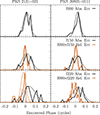 |
Fig. C.1. Normalised histograms of recovered phases (thick lines), t0, as well as phase differences, t0, ν1 − t0, ν2. The overlaid Gaussian curves (thin lines) have widths derived from the median absolute deviation of the distribution, which serve as estimates of the absolute and relative phase errors. The errors are listed in Table C.2. |
Results of phase shift uncertainty analysis using sine-wave injections into ACT AGN light curves.
For our ACT light curves, we can make progress on the empirical front using our preliminary catalog of 205 bright AGN multi-frequency light curves (see Sect. 2.1). Under the assumption that the Type A and Type B variations affect blazars that are not SMBHB candidates in the same way that they affect the two SMBHB candidates discovered thus far – which we note is untested – we estimated the absolute and relative phase shift uncertainties by injecting a sinusoid into the light curves:
 (C.1)
(C.1)
Here f is the original light curve, σf is the standard deviation of the original light curve, S/Nsin is the signal-to-noise ratio (S/N) of the sinusoid and P0 its period. When there were multiple measurements at the same MJD at the same frequency (i.e. from different arrays), we used their mean value. We factored the amplitude of the sinusoid into a S/N term (S/Nsin) and a noise term (σf) in order to use sine waves of similar S/N as our SMBHB candidates. Table C.1 shows the S/N of the sinusoids in our SMBHB candidates at each frequency, which we obtained by subtracting the best-fitting sinusoid from the SMBHB candidate, measuring the standard deviation of its residuals, σresid, and calculating
 (C.2)
(C.2)
where A is the best-fitting amplitude of the sine wave. In the same table, we also list the S/N of the residuals after subtracting the sine wave with respect to the flux uncertainties,
 (C.3)
(C.3)
where σf is the mean value of the flux uncertainties in the light curve. This variable captures the S/N of the non-sinusoidal residuals.
We estimated the uncertainty in phase measurements by fitting a sinusoid to f′(t),
![Mathematical equation: $$ \begin{aligned} s(t) = A\sin \left[\frac{2\pi (t - t_0)}{P_0}\right] + b, \end{aligned} $$](/articles/aa/full_html/2026/02/aa55047-25/aa55047-25-eq29.gif) (C.4)
(C.4)
where A, t0, and b are free parameters. A non-zero best-fitting t0 represents an error in recovering the input phase. We carried out this fit on our ensemble light curves (with the SMBHB candidates excluded from the sample), where the injected light curves had P0 and S/Nsin set to the values in Table C.1. We made two cuts on the ensemble of light curves. First, we required the time span covered by each light curve to be at least 95% that of PKS 2131–021 or PKS J0805 (see Table C.1) so that the length of the sine wave being fitted was representative of our SMBHB candidates. Second, we only included light curves which had S/Nvar < 5, where here, S/Nvar = σ/σf, with σ being the standard deviation of the original light curve. We explain the rationale for this cut in Appendix C.4. After both cuts, 10 to 18% of the original 204 light curves remainied, depending on the frequency and the AGN being studied (see ‘Count’ in Table C.2).
With the final ensemble in hand, we used the curve_fit() routine in the optimisation package of SCIPY to do a non-linear least squares fit to Eq. C.4 for each light curve and obtained a distribution of t0 at each of the ACT frequencies. The width of this distribution indicates the absolute error on the phase shift. The width of the distribution of the difference of the recovered fits in the light curves at two frequencies, Δtν1, ν2 = t0, ν1 − t0, ν2, indicates the relative error on the phase shifts between frequencies ν1 and ν2.
C.3. Results and discussion
The distributions of our phase fits are shown in Fig. C.1. We estimated the width of the distribution using the median absolute deviation (MAD) statistic, since it is robust to outliers, and report errors as σ = MAD/0.6745, where the numeric factor is the conversion to the Gaussian width for a normal distribution19. These error estimates are listed in Table C.2. There is broad agreement between the scenarios representing the two SMBHB candidates: the absolute uncertainty is about 3%, 5% and 6% of a cycle for 95, 147, and 225 GHz, respectively, and the relative uncertainty between 95 and 147 GHz is roughly 1.5% and is about 2–4% between 95/147 and 225 GHz.
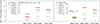 |
Fig. C.2. Relative errors calculated subject to various S/N values used in the sine waves injected into our ensemble of AGN light curves. Left: Relative errors obtained when S/Nsin was set to the value from PKS 2131–021 (heavy red lines) compared to when S/Nsin was set, at all frequencies, to 0, 1, 2, 3, or 5 (blue lines). Right: Relative errors obtained when AGN were cut from the sample based on their S/Nvar at 95 GHz (green lines), compared to what was obtained when all AGN were used (red lines). The dashed green line shows the results when both an S/Nvar < 5 cut was applied and S/Nsin was set to 3 at all frequencies. |
Generalised Lomb-Scargle test results of the optical light curves of PKS 2131–021.
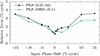 |
Fig. C.3. Effect of adding relative phase shifts into the injected sinusoids. Shown here is the 95–147 GHz relative error, where the sine wave injected into the 147 GHz light curve has been shifted relative to the 95 GHz light curve by the amount shown on the x-axis. The results for sine waves having properties of each of PKS 2131–021 and PKS J0805 (see Table C.1) are shown. |
The uncertainties from the MCMC fits (Sect. 3.1) are also shown in Table C.2. Here, we have assumed the hypothesis that the SMBHB light curves are dominated by Type A variations, such that the MCMC uncertainties represent purely relative errors, and have added in quadrature the uncertainties in ϕ0 provided in Tables 1 and 2 for the three pairs of ACT frequencies. The MCMC uncertainties are ∼2 times smaller than our empirical estimates. Given our current limited understanding of SMBHB light curve properties, we consider MCMC and empirical relative uncertainties to be in broad agreement. The MCMC uncertainties could be artificially low if Type B variations are non-negligble. On the other hand, the empirical analysis is based on the assumption that injecting sine waves into non-SMBHB AGN light curves provides an accurate simulation of SMBHB light curves, or, in other words, that Type A and Type B variations behave the same way in SMBHB and non-SMBHB AGN. If this assumption is faulty then the resulting errors could be inflated; furthermore, the sample size is rather small. For these reasons, the MCMC uncertainties may well be appropriate for SMBHBs, and they appear to be reasonable given the fit of the simple quadratic curve in Fig. 4. In the end, the main results of this paper are not sensitive to the exact size of the error bars, but the work in this appendix demonstrates the need for more data to better understand the uncertainties in SMBHB sine fits.
C.4. Further tests on phase uncertainty estimates
C.4.1. Varying S/Nsin:
The left panel of Fig. C.2 shows the effect on the relative uncertainties of varying the value of S/Nsin injected into the ensemble of light curves. Of particular interest is that the 95–225 GHz and 147–225 GHz uncertainties based on the fiducial S/Nsin values, taken from our real SMBHB candidate (Table C.1), are essentially the same if no sine wave is inserted into light curves in our ensemble, i.e. S/Nsin = 0. This means that our errors relative to the 225 GHz light curves, which only have S/Nsin ≈ 1, are dominated by Type A variations: it is not so much the phase shift in the sine wave that is being measured as the shift in the Type A variations. On the other hand, the 95–147 GHz relative uncertainty, where the SMBHB candidate has S/Nsin ≈ 2.5 − 3.5, is significantly smaller than if S/Nsin is set to zero. When S/Nsin is raised to 3 for light curves at all frequencies, the relative errors between all frequencies is ≈1%, and is reduced as S/Nsin increases, as expected.
C.4.2. Varying S/Nvar:
The right panel of Fig. C.2 explores how well the relative uncertainty can be measured for different S/Nvar. Our SMBHBs have comparatively small S/Nvar: at 95 GHz, S/Nvar = 3.8 and 2.0 for PKS 2131–021 and PKS J0805, respectively, compared to the median of 9.4 for the 204 other AGN in the ensemble. Effectively, this means that the residuals of the SMBHB candidates exhibit smaller variations than are found in the other, non-SMBHB light curves. As the figure shows, when all AGN were used to estimate the relative light curves, the errors relative to 225 GHz were higher than if we performed a cut on S/Nvar, such that the AGN included in the sample had variations that were more representative of the SMBHB candidates. On the other hand, the 95–147 GHz relative error is not sensitive to any cuts on S/Nvar. Again, the interpretation is that when S/Nsin ≳ 2, the sine wave is larger than the other variations, and thus the relative phase errors are not very sensitive to the non-sinusoidal variations; this is not the case when S/Nsin ∼ 1. With our limited sample, doing a cut for S/Nvar < 3 at 95 GHz, which would best represent our SMBHB candidates, would only leave 13 AGN in the sample. We therefore opted for a cut on S/Nvar < 5, which more than doubled the number of available AGN (see the ‘Count’ column in Table C.2) while not significantly altering the resulting error estimates, as can be seen in Fig. C.2. Finally, as a consistency check, for our fiducial cut of S/Nvar < 5 we also did a test where we set S/Nsin = 3 for all frequencies, and found results similar to the left-hand panel of Fig. C.2, where no cut on S/Nvar was used. This confirms the point made above, that when S/Nsin ≳ 2, non-sinusoidal variations do not impact the uncertainty much.
C.4.3. Including phase shifts in injected sine waves:
An inaccuracy in our empirical error estimates is that we injected sine waves with the same phase at all frequencies. In reality, we know from our two SMBHB candidates that they are slightly phase shifted. To test whether neglecting this effect affected our error estimates, we introduced different relative phase shifts into the injected sine waves and repeated the analysis. As for our fiducial error estimates, we applied a cut of S/Nvar < 5. Figure C.3 shows the results for the 95–147 GHz relative uncertainty, and demonstrates that it does have an effect on the error estimate. However, because the measured phase shifts between the ACT frequencies in our SMBHB candidates are smaller than 2%, corresponding to the central points along the x-axis in the figure, neglecting this effect in our fiducial results (Table C.2) only makes a modest difference. The results for the 95–225 GHz and 147–225 GHz uncertainties are considerably noisier but broadly similar20. In future estimates of the phase shift uncertainties, this effect should be taken into consideration.
Appendix D: Optical light curve periodicity
We analysed the joint CRTS V-band and ZTF g-band light curve of PKS 2131–021 with the generalised Lomb-Scargle (GLS) periodogram (Lomb 1976; Scargle 1982; Zechmeister & Kürster 2009). The strongest peak in the periodogram is at a period of 1711 days and a power of 0.22 (normalised between 0 and 1, where 1 would imply a perfect sine fit). The period is within the 3σ range, 1657.5–1854.1 days, of the periodicity detected in the OVRO 15 GHz data as reported in Table 1 of K25. The low GLS peak power is a result of the strong red-noise component in the data. We estimated21 a power-law index of βopt = 1.5 of the red-noise power spectral density (PSD ∼ν−β, where ν is the temporal frequency). Compared to the 15 GHz radio light curve with a PSD index βradio = 1.8 (O22), the optical PSD is flatter, implying stronger variability on short timescales.
GLS analysis of the joint CRTS and ZTF g-band data gave a period of 1711 days and a power of 0.22. ZTF alone gave a period of 1728 days and a power of 0.23 whereas CRTS alone did not identify a period consistent with the radio period. In fact, the strongest peaks in the CRTS periodogram came from the sampling window associated with the CRTS observing cadence. The effect of the CRTS cadence can be demonstrated by downsampling the ZTF data (median Δt = 3 days) to the CRTS cadence (median Δt = 15 days): a joint analysis gave a period of 1724 days and a power of 0.36 but the false alarm probability (FAP) from bootstrap analysis shows the result was no longer significant. Although the FAP is not relevant for assessing the statistical significance of any peak against a correlated noise background, it can be used to assess the effect of cadence on a signal. In this case, the shorter cadence of ZTF data improves the statistical detectability of a signal in the joint data to a significant level, with a p-value of 0.002, as compared to a p-value of 0.414 for joint data with the same median cadence.
We performed four different tests to evaluate the feasibility of using optical data to robustly detect sinusoidal variations in PKS 2131–021.
D.1. Test 1:
We used the procedure described in Appendix A of O22 to estimate the significance of the detected periodicity. Our null hypothesis was that the detected periodicity was a spurious result of a pure red-noise stochastic process. We simulated 20 000 artificial light curves that had the same PSD, probability distribution function, time sampling and observational noise characteristics as the optical light curve. We used the lcsim Python package (Kiehlmann 2023) based on the algorithm of Emmanoulopoulos et al. (2013). For the original data and each simulation we calculated the GLS periodogram, identified the strongest peak, and used the remaining simulations to estimate the probability that the red-noise process produced a power at least as strong as detected at the peak frequency. This probability was used as test statistic in the next analysis step. Among all simulations we counted those that had a test statistic at least as low as that derived from the original light curve, which gave us the global p-value. This global p-value takes into account that spurious periodic signals may occur at any frequency in the frequency range tested by the GLS periodogram. We refer to Appendices A in O22 and D25 for a detailed description of the procedure. We found a global p-value of 0.937. Therefore, we cannot reject the null hypothesis of a red-noise process producing a spurious periodicity.
D.2. Test 2:
When we take our prior knowledge of the strongly significant radio periodicity (p-value = 5.3 × 10⁻⁷; K25) into account, we can ask the following question: How likely is it that the red-noise process produces a GLS peak at least as strong as observed in the optical data with a period in the 3σ range of the radio period (1657.5–1854.1 days, K25)? Among the 20 000 simulations we counted 934 that fulfil these criteria, corresponding to a p-value of 0.047. Even with the optical period falling close to the radio period, we cannot confidently rule out the red-noise hypothesis.
Stronger support for the true existence of a period in the optical data consistent with the period seen in the radio data comes from the fact of how well the phase of the optical periodicity ties into the phase-frequency relation discussed in K25.
D.3. Tests 3 and 4:
We also analysed the CRTS and ZTF data independently. The GLS periodogram of the ZTF data shows the strongest peak at a period of 1728 days. The periodogram of the CRTS also shows a peak near the radio periodicity. However, there are several other spurious peaks that do not correspond to significant detections. Using the same approach as for Test 2 above on the individual light curves, in Table C.3 we see that the combined CRTS+ZTF light curve provides the most evidence against the null hypothesis. This is expected as the joint data cover more cycles of the long timescale periodicity, hidden in the red-noise component, that produces strong variability on shorter timescales.
The foregoing analyses demonstrate that it can be more complicated to detect a periodicity in optical blazar light curves from current surveys, since the short-term variability is stronger than at radio and submm frequencies. Thus more extended long-term observations with higher cadence are needed to reveal periodicities in the presence of the red-noise component
All Tables
Results of phase shift uncertainty analysis using sine-wave injections into ACT AGN light curves.
Generalised Lomb-Scargle test results of the optical light curves of PKS 2131–021.
All Figures
|
Fig. 1. PKS 2131–021 light curves from OVRO, ACT, and ALMA. Heavy points are binned into 50-day intervals (100 for OVRO) to guide the eye, with individual measurements shown as lighter points. Sinusoidal fits, shown with the continuous curves, were done on the unbinned data. The sine fits for ALMA are from K25 and sine fits to ACT were done for this paper (see text). For the OVRO data, the solid curve is the best fit for the ACT time range, while the dashed sine curve corresponds to the ALMA time range. A monotonic phase shift of the sine waves to earlier times with increasing frequency is visible by eye, and is reported relative to the OVRO phase as Δϕ0 in Tables 1 and B.1. |
| In the text | |
|
Fig. 2. Correlation of medium-term flux density variations in ALMA and ACT light curves of PKS 2131–021. Top: ALMA 91.5 GHz and ACT 95 GHz (PA5) light curves that have been filtered by binning and subtracting a long timescale trend. The binning is in five day chunks, and only time chunks containing data from both ALMA and ACT are retained. The long timescale trend was removed by fitting a third-degree B-spline with 120-day knot spacing to each binned light curve and subtracting; this effectively acts as a high-pass filter of variations on timescales ≳120 days, removing the large sinusoidal pattern. Clear correlations between the light curves are seen on these timescales. Bottom: Pearson correlation between the filtered ALMA and ACT light curves, for different spline knot spacings. Errors were estimated by calculating the correlations between the ALMA PKS 2131–021 light curve and each of the other 204 ACT light curves in our bright AGN library, which should be uncorrelated, and taking the standard deviation. The thick coloured point at 120 days corresponds to the data shown in the upper panel. |
| In the text | |
|
Fig. 3. PKS J0805–0111 light curves at 15 GHz, 95 GHz, 147 GHz, and 225 GHz. The main panel shows the time range covered by the ACT observations, while the inset shows the full range observed by OVRO. Heavy points are binned into 25-day intervals (100 days in the inset) to guide the eye, with individual measurements shown as lighter points; the sinusoidal least-squares fits were done on the unbinned data. A monotonic phase shift of the sine waves to earlier times with increasing frequency is visible by eye, and is reported relative to the OVRO phase as Δϕ0 in Table 2. The dashed vertical line at MJD 59041 (2020 July 11) indicates the approximate date at which D25 found that the sinusoidal variation in the 15 GHz ceases. The ACT mm data also apparently flatten around the same time. |
| In the text | |
|
Fig. 4. PKS 2131–021 phase shifts measured by ACT at 95, 147, and 225 GHz (black points), compared to the phase shift results of K25 (blue points); see Table 3. We note that the ACT 95 GHz and ALMA 91.5 GHz points overlap. The Haystack or OVRO 15 GHz light curves provided the phase reference in all cases. Uncertainties were determined by the MCMC sine-wave fits (Eq. (1)). The curved blue line shows the quadratic fit determined by K25 (Eq. (3)). The orange line is the best-fit power law to the Haystack, ALMA, and ACT data (Eq. (4), Table 5). |
| In the text | |
|
Fig. 5. Posterior probabilities of the power-law MC fit to the sinusoid phase shifts (Eq. (4)) for different data combinations. The contours show the 95% credible regions and the dots are the maximum likelihood values (cf. Table 5). Flat priors on a and b in the ranges of (0.05, 4) and (−2, −0.05) were used. |
| In the text | |
|
Fig. 6. Phase shifts of the ACT best-fit sinusoids relative to the OVRO 15 GHz light curves for each of PKS 2131–021 and PKS J0805–0111. The lines are the best fits to the power law of Eq. (4), with only ACT data included. The best-fitting values are listed in Table 5. The heavy error bars are the fiducial uncertainties of the phase shifts from the MCMC fits (Sect. 3.1) relative to 15 GHz, while the light error bars show an empirically derived, relative phase uncertainty between 95 GHz and 147–225 GHz (see Appendix C.1). Fits were done with the fiducial uncertainties. The PKS J0805–0111 points have been shifted slightly to the right for ease of viewing. |
| In the text | |
|
Fig. 7. A 2D slice through the wind-collimated jet, illustrating the MKO model. The relativistic flow velocity, β, at a particular point in the jet is parallel to the local wind velocity, βw. The wind propagates semi-ballistically, so different distances along the jet have local wind velocity directions out of phase. Since it is the aberration caused by the changing jet velocity that modulates the observed flux, frequencies originating from different locations in the jet that are observed simultaneously are at different phases in their sinusoidal flux variations. |
| In the text | |
|
Fig. 8. Comparison of radio and optical light curves of PKS 2131–021. The sine waves shown in the figure come from Tables 1 and 4 of K25 for the radio and ZTF optical data, respectively. The fit to the ZTF data has been extrapolated back in time to show that the cadence of the CRTS is not sufficient to easily discover this sinusoidal pattern (see text for additional details). |
| In the text | |
|
Fig. C.1. Normalised histograms of recovered phases (thick lines), t0, as well as phase differences, t0, ν1 − t0, ν2. The overlaid Gaussian curves (thin lines) have widths derived from the median absolute deviation of the distribution, which serve as estimates of the absolute and relative phase errors. The errors are listed in Table C.2. |
| In the text | |
|
Fig. C.2. Relative errors calculated subject to various S/N values used in the sine waves injected into our ensemble of AGN light curves. Left: Relative errors obtained when S/Nsin was set to the value from PKS 2131–021 (heavy red lines) compared to when S/Nsin was set, at all frequencies, to 0, 1, 2, 3, or 5 (blue lines). Right: Relative errors obtained when AGN were cut from the sample based on their S/Nvar at 95 GHz (green lines), compared to what was obtained when all AGN were used (red lines). The dashed green line shows the results when both an S/Nvar < 5 cut was applied and S/Nsin was set to 3 at all frequencies. |
| In the text | |
|
Fig. C.3. Effect of adding relative phase shifts into the injected sinusoids. Shown here is the 95–147 GHz relative error, where the sine wave injected into the 147 GHz light curve has been shifted relative to the 95 GHz light curve by the amount shown on the x-axis. The results for sine waves having properties of each of PKS 2131–021 and PKS J0805 (see Table C.1) are shown. |
| In the text | |
Current usage metrics show cumulative count of Article Views (full-text article views including HTML views, PDF and ePub downloads, according to the available data) and Abstracts Views on Vision4Press platform.
Data correspond to usage on the plateform after 2015. The current usage metrics is available 48-96 hours after online publication and is updated daily on week days.
Initial download of the metrics may take a while.