| Issue |
A&A
Volume 706, February 2026
|
|
|---|---|---|
| Article Number | A118 | |
| Number of page(s) | 12 | |
| Section | Planets, planetary systems, and small bodies | |
| DOI | https://doi.org/10.1051/0004-6361/202555227 | |
| Published online | 05 February 2026 | |
Response of Venusian plasma environment to the interplanetary coronal mass ejections on 5 November 2011: A magnetohydrodynamics simulation study
1
Deep Space Exploration Laboratory/School of Earth and Space Sciences, University of Science and Technology of China,
Hefei,
China
2
Department of Earth Sciences, the University of Hong Kong, Pokfulam,
Hong Kong
SAR,
China
3
Institute of Space Science and Applied Technology, Harbin Institute of Technology,
Shenzhen,
China
4
Space Research Institute, Austrian Academy of Sciences,
Graz,
Austria
★ Corresponding author: This email address is being protected from spambots. You need JavaScript enabled to view it.
Received:
21
April
2025
Accepted:
24
November
2025
Abstract
Context. As an unmagnetized planet, Venus lacks an intrinsic magnetic field, leading to the direct interaction with the solar wind, which results in differences in physical processes within its magnetosphere–ionosphere (MI) system compared to Earth. With intense solar wind disturbances, it has been suggested that interplanetary coronal mass ejections (ICMEs) have a pronounced effect on Venus.
Aims. This study aims to investigate the responses of the Venusian plasma environment to ICMEs. A simulation driven by a real ICME event that occurred on 5 November 2011, was conducted to systematically and quantitatively analyze the plasma processes in Venusian magnetosphere. During this event, the solar wind dynamic pressure at the model input increased by a factor of up to 4.8, while the interplanetary magnetic field (IMF) strength was enhanced by a factor of 1.9.
Methods. The numerical simulation for Venusian plasma environment uses a multi-fluid global magnetohydrodynamics (MHD) model, coupled with the uniform neutral atmosphere. Utilizing the upstream magnetic field data from VEX and idealized solar wind plasma parameters as model inputs, we examine the response of Venusian plasma environment after the ICME arrival.
Results. Venusian plasma environment and boundaries respond rapidly on the order of minutes. During the ICME, the subsolar bow shock location exhibits an inverse-linear proportionality to the fast magnetosonic Mach number. Meanwhile, the variation in boundaries’ locations demonstrates that high solar wind dynamic pressure and an enhanced IMF display compressive and expanding effects, respectively. The total integral of the ions’ escape rate shows that under ICME passage, the O+ escape rate of Venus exhibits a sustained increase, from 6.0 × 1024 s−1 to 3.0 × 1025 s−1. Both solar wind dynamic pressure and IMF strength enhance ion escape, with dynamic pressure dominating this process.
Conclusions. The simulation driven by a real ICME event demonstrates severe, rapid, and complex responses of Venusian plasma environments, accompanied by an order-of-magnitude enhancement O+ escape rate. These results could advance the understanding of the long-term evolution of terrestrial planets and provides references for the scientific targets of future missions.
Key words: magnetohydrodynamics (MHD) / methods: numerical / planets and satellites: atmospheres / planets and satellites: magnetic fields / planets and satellites: terrestrial planets
© The Authors 2026
 Open Access article, published by EDP Sciences, under the terms of the Creative Commons Attribution License (https://creativecommons.org/licenses/by/4.0), which permits unrestricted use, distribution, and reproduction in any medium, provided the original work is properly cited.
This article is published in open access under the Subscribe to Open model. This email address is being protected from spambots. You need JavaScript enabled to view it. to support open access publication.
1 Introduction
Venus shares a similar size, mass and Sun-planet distance to the Earth within the Solar System, arousing considerable interest in explorations of planetary evolution and the formation of habitability (Donahue & Russell 1997; Way et al. 2016). However, unlike Earth, Venus has an exceptionally dry and dense atmosphere, which is attributed to several processes, particularly volatile release into the atmosphere, surface-gas reactions, and atmospheric escape driven by solar wind (Gillmann et al. 2022). Consequently, Venusian interaction with the solar wind attracts significant interest and has been widely studied using data from several previous missions. Due to the absence of an intrinsic magnetic field (Phillips & Russell 1987), Venus interacts with upstream solar wind more directly (Luhmann 1986), generating the so-called induced magnetosphere whose appearance is often described as draping. This draping magnetic field is formed as the solar wind, together with the frozen magnetic field, slows down around Venus due to the influence of mass loading (McComas et al. 1986; Rong et al. 2014; Futaana et al. 2017).
Interplanetary coronal mass ejections (ICMEs), the interplanetary counterparts of coronal mass ejections, represent the most common large-scale disturbances from the solar corona. They are characterized by high plasma dynamic pressures and an enhanced interplanetary magnetic field (IMF), for which the response of planetary spaces has always been of great interest. Although ICMEs impacting Venus have been detected by missions such as Pioneer Venus Orbiter (PVO) and Venus Express (VEX) (McEnulty et al. 2010; Edberg et al. 2011; Collinson et al. 2015; Dimmock et al. 2018; Xu et al. 2019), the available observations remain sparse. This limitation arises primarily from the particularly sparse density and velocity data from VEX ASPERA-4/IMA and the polar orbit of VEX, which resulted in low spatial coverage in the solar wind. Due to these observational constraints, previous studies have mostly focused on the Venusian space environment under typical quiet solar wind, with limited systematic and quantitative investigation dedicated to its response under such intense space weather events. The prior dominance of solar wind interaction, however, suggests that the Venusian plasma system (magnetosphere–ionosphere) is likely to experience severe alterations during solar activities such as ICMEs and corotating interaction regions (CIRs) (Knudsen 1988; Russell et al. 2006; McEnulty et al. 2010; Futaana et al. 2017; Chang et al. 2018). Hence, it has been suggested that intense solar wind disturbances play a more important role in controlling the plasma environment, thereby influencing the evolution of unmagnetized planets (Luhmann et al. 2007; Edberg et al. 2010; Xu et al. 2019; Rout et al. 2024). For instance, Edberg et al. (2011) statistically examined the response of Venusian atmospheric escape to 147 CIR and ICME events during solar minimum, reporting an average 1.9-fold increase in the ion escape rate compared to in quiet conditions. Moreover, it has been inferred that in the early Solar System ICMEs were more powerful due to higher solar wind density, velocity, and stronger EUV flux (Wood et al. 2005; Ribas et al. 2005), which would have intensified these effects. Therefore, ICMEs are expected to strongly influence the Venusian plasma environment, particularly in enhancing ion loss, which may imply Venusian long-term water evolution and lead to an extremely arid environment (Barabash et al. 2007a).
Global numerical models are effective tools for simulating the interaction between the Venusian magnetosphere–ionosphere (MI) system and the solar wind, which can provide reasonable global data for studying the changes of the Venusian space environment under different upstream conditions and interpreting the limited observations (Chen et al. 2025a,b; Dang et al. 2023; Zhao et al. 2025). Dimmock et al. (2018) applied a hybrid model to investigate the response of the Venusian plasma environment during the passage of an ICME and mainly studied the morphology of draping magnetic field lines and the relative change in the ion escape rate under the influence of ICME. However, their simulations were performed under constant upstream conditions. Given dramatically variable upstream conditions during the ICME, studying the Venusian MI response to time-varying upstream driving is necessary to clearly understand the realistic effects of ICMEs.
This paper applies a time-dependent multi-fluid global magnetohydrodynamics (MHD) model to study the magnetospheric and ionospheric response of Venus under a realistic ICME event on 5 November 2011, which is the largest ever observed at Venus (Dimmock et al. 2018; Xu et al. 2019). The simulation is driven by time-varying IMF data observed by VEX and provides a global view of the variations within the MI system. Furthermore, we calculated the escape rate of major heavy ions in the Venus atmosphere and estimated quantitatively the relative contributions of enhancement of both dynamic pressure and IMF strength during the ICME passage. This study could provide insights into the physical mechanisms of the global variation in the Venusian magnetosphere and ion escape under ICME, as well as insights into other unmagnetized planets.
2 3D multi-fluid MHD model
2.1 Model description
This paper uses a multi-fluid, high-resolution global MHD model to simulate the interaction between the Venusian MI system and the solar wind (Dang et al. 2023). By utilizing averaged upstream magnetic field data from VEX as inputs, Dang et al. (2023) simulated the Venusian plasma environment. The simulated magnetic field structures showed a remarkable correspondence with those observed by VEX near Venus. This model is also capable of capturing small-scale structure, such as the Kelvin-Helmholtz instability and turbulent structures (Dang et al. 2022, 2025). The model solver was built on high-order numerical algorithms with a high-resolving power: GAMERA (Grid Agnostic MHD for Extended Research Applications) (Zhang et al. 2019), which allowed us to enable more reasonable Venusian responses to upstream conditions and to analyze the dynamic mechanisms of oxygen ion escape. In the code, a seventh-order upwind reconstruction was employed to compute the numerical fluxes at cell interfaces. Additionally, a high-order constraint transport method was utilized to maintain the divergence-free magnetic field. Using the original multi-fluid equations used by Brambles et al. (2010), the multi-fluid Venus model solves the continuity, momentum, and energy conservation equations of four main ions in the Venusian ionosphere (H+, O+, ![Mathematical equation: $\[\mathrm{O}_{2}^{+}\]$](/articles/aa/full_html/2026/02/aa55227-25/aa55227-25-eq1.png) , and
, and ![Mathematical equation: $\[\mathrm{CO}_{2}^{+}\]$](/articles/aa/full_html/2026/02/aa55227-25/aa55227-25-eq2.png) ), as well as the magnetic induction equations with consideration of plasma resistivity:
), as well as the magnetic induction equations with consideration of plasma resistivity:
![Mathematical equation: $\[\frac{\partial \rho_i}{\partial t}+\nabla \cdot\left(\rho_i \boldsymbol{u}_i\right)=S_i-L_i\]$](/articles/aa/full_html/2026/02/aa55227-25/aa55227-25-eq3.png) (1)
(1)
![Mathematical equation: $\[\begin{aligned}& \frac{\partial\left(\rho_i \boldsymbol{u}_i\right)}{\partial t}+\nabla \cdot\left(\rho_i \boldsymbol{u}_i \boldsymbol{u}_i+p_i \boldsymbol{I}\right)+\boldsymbol{F}_i^d=\rho_i \boldsymbol{G}-\rho_i \sum_n v_{i n} \boldsymbol{u}_i-L_i \boldsymbol{u}_i \\& \frac{\partial \epsilon_i}{\partial t}+\nabla \cdot\left[\boldsymbol{u}_i\left(\epsilon_i+p_i\right)\right]+\boldsymbol{u}_i \cdot \boldsymbol{F}_i^d=\rho_i \boldsymbol{u}_i \cdot \boldsymbol{G}+\rho_i \sum_n \frac{v_{i n} \boldsymbol{u}_i}{m_i+m_n}.\end{aligned}\]$](/articles/aa/full_html/2026/02/aa55227-25/aa55227-25-eq4.png) (2)
(2)
![Mathematical equation: $\[\left[3 k\left(T_n-T_i\right)-m_i u_i^2\right]-\frac{1}{2} L_i u_i^2+\frac{k}{\gamma-1}\left(\frac{S_i T_n-L_i T_i}{m_i}\right)\]$](/articles/aa/full_html/2026/02/aa55227-25/aa55227-25-eq5.png) (3)
(3)
![Mathematical equation: $\[\frac{\partial \boldsymbol{B}}{\partial t}=\nabla \times(\boldsymbol{u} \times \boldsymbol{B}-\eta \boldsymbol{J})\]$](/articles/aa/full_html/2026/02/aa55227-25/aa55227-25-eq6.png) (4)
(4)
![Mathematical equation: $\[\mu_0 \boldsymbol{J}=\nabla \times B\]$](/articles/aa/full_html/2026/02/aa55227-25/aa55227-25-eq7.png) (5)
(5)
where i and n indicate, respectively, the ion and neutral species. ρi, ui, pi, Ti and ϵi are the plasma parameters: the mass density, velocity, pressure, temperature, and energy of the ion species, i. Si and Li are the ion production rates and loss rates, respectively. I in Equation (2) is the unit tensor. In Equations (2) and (3), ![Mathematical equation: $\[\boldsymbol{F}_{i}^{d}\]$](/articles/aa/full_html/2026/02/aa55227-25/aa55227-25-eq8.png) is the electromagnetic force exerting on the ion species, i, and G is the vector of gravitational acceleration. For ionospheric photochemistry and collision terms, k represents the Boltzmann constant, Tn denotes the neutral temperature, γ is the adiabatic index, mi and mn are the mean molecular mass of ion species i and neutral species n, νin stands for the ion–neutral collision frequency, and u refers to the bulk velocity. In Equation (4), B is the vector of the magnetic field, η is the magnetic resistivity, and J is the electric current, which was calculated with Ampère’s law. μ0 is the vacuum permeability. In this model, the electron pressure has been neglected. Considering the small ions’ gyroradii around Venus compared to its scale, the Hall effects are also neglected (Ledvina et al. 2008).
is the electromagnetic force exerting on the ion species, i, and G is the vector of gravitational acceleration. For ionospheric photochemistry and collision terms, k represents the Boltzmann constant, Tn denotes the neutral temperature, γ is the adiabatic index, mi and mn are the mean molecular mass of ion species i and neutral species n, νin stands for the ion–neutral collision frequency, and u refers to the bulk velocity. In Equation (4), B is the vector of the magnetic field, η is the magnetic resistivity, and J is the electric current, which was calculated with Ampère’s law. μ0 is the vacuum permeability. In this model, the electron pressure has been neglected. Considering the small ions’ gyroradii around Venus compared to its scale, the Hall effects are also neglected (Ledvina et al. 2008).
The photochemical processes for four major ions in the Venusian ionosphere are considered in this model, including H+, O+, ![Mathematical equation: $\[\mathrm{O}_{2}^{+}\]$](/articles/aa/full_html/2026/02/aa55227-25/aa55227-25-eq9.png) and
and ![Mathematical equation: $\[\mathrm{CO}_{2}^{+}\]$](/articles/aa/full_html/2026/02/aa55227-25/aa55227-25-eq10.png) . The corresponding neutral species at Venus are adapted from Fox & Sung (2001). In this study, we set the neutral atmosphere to be uniform with respect to the solar zenith angles. More information about the model is available in the referenced paper (Dang et al. 2023).
. The corresponding neutral species at Venus are adapted from Fox & Sung (2001). In this study, we set the neutral atmosphere to be uniform with respect to the solar zenith angles. More information about the model is available in the referenced paper (Dang et al. 2023).
The Venus solar orbital (VSO) coordinate system was applied for the model, whose X-axis is along the Venus-Sun line and Z-axis is aligned with the direction of Venusian orbital angular momentum. Then we get Y-axis by right-hand rule. This study uses a 64 × 64 × 64 computational grid divided in radial, polar, and azimuthal directions and an output time interval of 0.1 minute to simulate the variation in the Venusian space environment. The 0.1 minute interval was chosen to resolve the minute-scale global response of the Venusian MI system (Slavin et al. 2009). This interval also aligns with our model’s normalized time of approximately 1 minute. The low altitude boundary of the grid was set to be 100 km above the Venus surface. A spherical grid, extending from 100 to 500 km above the surface, was used as the Venusian ionosphere, with a radial resolution of 20 km. Above 500 km, an ellipsoid grid surrounds the spherical ionosphere, with its size increasing gradually with the radial distance. The outer boundaries of the X, Y, and Z axes were set to be between [−10, 4], [−6, 6], and [−6, 6] in the unit of Venus radii (RV), respectively. We assumed a hard wall at the inner boundary for ion velocity to prevent any plasma mass flux from crossing the inner boundary, and applied a zero-gradient condition for the magnetic field at the inner boundary. Moreover, we applied a zero-gradient condition for the densities and temperatures of ions at the outer boundary, while the outer boundary condition of H+ was controlled by the solar wind parameters.
The GAMERA MHD solver of our model has been extensively validated in previous studies. Importantly, this solver has demonstrated strong applicability to simulations under time-varying upstream conditions (Hudson et al. 2021; Burkholder et al. 2024). For instance, Hudson et al. (2021) employed the solver to reproduce the Earth’s response to both ICMEs and CIRs, confirming that the model framework can capture well the magnetospheric response to changing driving conditions. Therefore, our model is also capable of handling the variations of Venusian plasma environment under variable upstream conditions.
2.2 Solar wind input of the model during the ICME event on 5 November 2011
An ICME impacting Venus was detected by VEX from its leading shock on 5 November 2011, clearly visible from a sharp increase in the magnetic field gradient followed by an overall increase in the magnetic field strength downstream (Vech et al. 2015; Dimmock et al. 2018; Xu et al. 2019). Based on the magnetic field and ion and electron energy spectrum from VEX, the ICME reached the vicinity of Venus at around 03:40 UT, with VEX encountering the bow shock (BS) at 07:00 UT. The space-craft orbit is shown in Figure 1a, from 00:00 UT to 10:20 UT on 5 November 2011. The orbital track is presented in a cylindrical coordinate plane in Figure 1a1, whose two axes correspond to X and ![Mathematical equation: $\[\sqrt{\mathrm{Y}^{2}+\mathrm{Z}^{2}}\]$](/articles/aa/full_html/2026/02/aa55227-25/aa55227-25-eq11.png) . The colored lines represent various regions traversed by VEX from the solar wind to the region inside the BS. With VEX having an elliptical polar orbit, the X-Z plane trajectory is plotted in Figure 1a2.
. The colored lines represent various regions traversed by VEX from the solar wind to the region inside the BS. With VEX having an elliptical polar orbit, the X-Z plane trajectory is plotted in Figure 1a2.
The simulation is driven by IMF measurements from VEX to replicate realistic ICME conditions, i.e., data from 03:40 UT to 05:40 UT on 5 November 2011. Since the solar wind plasma data measurements from direct instrument on that day were nearly unavailable, the solar wind plasma parameters of driving conditions are idealized to typical linear variations. Figure 1b shows the driving conditions throughout the simulation, including IMF components in the X, Y, and Z directions and solar wind plasma velocity, temperature, and density (plotted from top to bottom). To initialize the model to achieve a stable state, we started the simulation under typical quiet solar wind conditions near Venus for the first 5 minutes, without any magnetic field, as is shown in Figures 1b4 and b5. The solar wind was set to Vx = 400 km/s, Vy = Vz = 0, and has a density of 10 cm−3 and a temperature of 105 K. Subsequently, the simulation under quiet solar wind ran for an additional 35 minutes, maintaining the plasma parameters and introducing the IMF. The magnetic field components Bx, By, and Bz were set to constant values of [3.69, 2.48, −7.46] nT, based on the last quiet upstream magnetic field measurement by VEX before the arrival of ICME. After initialization, upstream driving of the ICME was applied for a duration of 120 minutes. The magnetic field components were taken from VEX observations, corresponding to the period marked by the red line in the VEX trajectory shown in Figure 1a1. As is shown in Figures 1b1–b3, the ICME dramatically enhances the magnetic field strength and induces sustained rotation in IMF orientation. We applied a reasonable idealized solar wind plasma property as driving conditions (Futaana et al. 2017; Rout et al. 2024; Dimmock et al. 2018). The solar wind plasma has been accelerated to 680 km/s following the ICME, which is consistent with observations (Rout et al. 2024). Upon the ICME arrival, both the number density and temperature dramatically increase to 15 cm−3 and 106 K, respectively. The density and temperature ratios for ICME and quiet conditions are derived from driving conditions of Dimmock et al. (2018) simulations, which incorporate ICME shock observations from VEX. Subsequently, the number density continues to increase gradually, reaching 19 cm−3 during the ICME event, while the temperature decreases gradually to 8.5 × 10⁵ K. The trends of velocity, density, and temperature closely resemble driving setting in an MHD simulation study of Martian response to ICME (Ma et al. 2017). For details on the changes in ICME plasma parameters, refer to Figures 1b4 and b5.
3 Model results
3.1 Magnetospheric response
The ICME event was preceded by a strong shock that reached Venus around 03:40 UT on 5 November, showing a dramatic increase of the magnetic field (see Figures 1b1–b3). Figure 2 illustrates the changes in the Venusian plasma environment during the passage of the ICME shock from the MHD model. The left and right columns of Figure 2 show contour plots of magnetic field strength and plasma bulk velocity in the Venus X–Z plane (VSO coordinate system). From top to bottom are parameters at different simulation times (38, 39, 41, and 42 minutes), presenting their responses to the ICME shock and subsequent variations. The first row in Figure 2 corresponds to the time right before ICME shock arrival. The Venusian BS and induced magnetosphere boundary (IMB) are structured as is expected under quiet solar wind. As with a typical Venusian space environment, the IMF piles up and drapes around the Venus obstacle within the magnetosheath. The magnetic barrier is thus formed to prevent the solar wind from penetrating the ionosphere, whose maximum strength exceeds 60 nT. As the solar wind approaches Venus, the plasma flow slows down and diverts around the planet. The ICME shock arrives at Venus at 39 minutes, carrying a much faster flow and stronger IMF as is shown in Figures 2a2 and b2. The ICME shock causes an immediate response in the magnetosheath, causing the average magnetic field strength along the subsolar line to jump from approximately 44 nT to 66 nT. Two minutes later, the ICME shock front has passed Venus, with the plasma environment reaching a quasisteady state. As is shown in the third row of Figure 2, the IMF strength at this time decreased to 8.9 nT. The plasma environment around the planet is significantly changed by the shock, mainly driven by the high-temperature, high-density solar wind. The increased solar wind kinetic energy is converted into magnetic energy within the magnetic barrier, significantly enhancing the magnetic field strength. It can be seen that the magnetic strength close to the inside of BS is enhanced from 20 nT at 38 min to 30 nT. Meanwhile, the elevated dynamic pressure leads to a significant compression of the magnetotail compared to the quiet period. From Figure 2b3, the magnetotail at X = −2 RV is compressed to a size smaller than that of the planet. At 42 minutes, Venus is influenced by stronger IMF carried by the ICME. In order to impede the penetration of enhanced IMF, the magnetic field strength across the entire magnetic barrier increases to over 60 nT. In the nightside flank region, with coordinates in the range of X ~ [−1, 0] RV and at Z ~ ±1.1 RV, the plasma flow velocity is over 800 km/s, higher than solar wind. The plasma acceleration is likely to be driven by the intensified J × B force. The snapshots of the Venusian space environment clearly show a rapid response to the ICME shock, with a timescale on the order of minutes.
Based on the analysis of magnetic field strength and velocity distribution, we further investigated the magnetic topology by examining its three components. Fig 3 shows the three components of magnetic field in Venus space environment before and under ICME impact. Panel (a1) shows that Bx exhibits a strong bipolar pattern, with positive values on the +Z side and negative values on the −Z side, indicating the draping of the IMF around Venus. Panel (b1) reveals that By remains relatively weak and symmetric, suggesting that the IMF contribution in the Y direction is minor under these conditions. In contrast, panel (c1) shows that Bz displays an enhancement near the magnetic barrier on the dayside. A clear polarity reversal is observed downstream in panels (a1), (b1), and (c1), reflecting the typical IMF draping pattern around the unmagnetized body in night side. As draped field lines are carried tailward, portions closest to the planet remain anchored, forming the observed reversal structure. Upon arrival of the ICME shock, the dayside magnetic field components By and Bz exhibit enhancement, as is illustrated in panels (b2)–(c2). As the IMF clock angle evolves, panels (a3)–(b3) reveal a distinct reorganization in the spatial distribution of these components. The variations in these components clearly illustrate both a strengthening of the field and a rotation of the magnetosphere. For magnetic barrier zone, the maximum of the By component increases from 29.3 nT at 38 min to 166.5 nT at 42 min, and the Bz component increases from 88.5 nT at 38 min to 166.9 nT at 42 min. Due to a fast response to the solar wind condition, the Venus magnetosphere rotation corresponds to the variation in the IMF clock angle. The arrival of the ICME enhances the |By|/|Bz| ratio, signifying a strengthening of the By component relative to Bz. The induced magnetosphere exhibits a corresponding enhancement in the By component and a decrease in the Bz component, comparing panels (b1,c1) with (b4, c4) in Fig. 3. Meanwhile, panel (a4) illustrates the rotation of the magnetotail lobes. This rotation is evidenced by a significant weakening of the magnetic field pileup in the X–Z plane, which implies that the induced magnetic poles have shifted substantially close to it.
In Figure 2, the solar wind dynamic and magnetic pressure are shown to play a crucial role in the changes of plasma boundaries’ locations and magnetic barrier size. Here, we discuss the detailed changes in plasma boundaries (BS and IMB) under ICME. The subsolar BS and IMB locations are defined as the equilibrium positions where plasma dynamic pressure equals thermal pressure and where plasma thermal pressure equals magnetic pressure, respectively (Xu et al. 2021). Figure 4 shows snapshots of the attitude profiles of the thermal, magnetic, and dynamic pressure along the subsolar line in the simulation. The selected event is at solar minimum, when the magnetic barrier field diffuses inward and the ionosphere becomes magnetized (Zhang et al. 2008; Futaana et al. 2017). Figure 4a represents the pressure profiles under typical quiet solar wind conditions, with a low solar wind dynamic pressure of 2.7 nPa. As the pressures vary, the structure of Venus space environment is clearly shown. The BS is located at 1.33 RV. The IMB is positioned at 1.11 RV. The region below the IMB is magnetized, with a maximum magnetic pressure of 3.5 nPa. Intensive photochemical reactions occur in the Venusian ionosphere. At lower altitudes, the primary ionization of CO2 swiftly produces ![Mathematical equation: $\[\mathrm{CO}_{2}^{+}\]$](/articles/aa/full_html/2026/02/aa55227-25/aa55227-25-eq13.png) , which is then rapidly transformed into
, which is then rapidly transformed into ![Mathematical equation: $\[\mathrm{O}_{2}^{+}\]$](/articles/aa/full_html/2026/02/aa55227-25/aa55227-25-eq14.png) via fast reactions:
via fast reactions: ![Mathematical equation: $\[\mathrm{CO}_{2}^{+}\]$](/articles/aa/full_html/2026/02/aa55227-25/aa55227-25-eq15.png) + O →
+ O → ![Mathematical equation: $\[\mathrm{O}_{2}^{+}\]$](/articles/aa/full_html/2026/02/aa55227-25/aa55227-25-eq16.png) + CO and
+ CO and ![Mathematical equation: $\[\mathrm{CO}_{2}^{+}\]$](/articles/aa/full_html/2026/02/aa55227-25/aa55227-25-eq17.png) + O → O+ + CO2/O+ + CO2 →
+ O → O+ + CO2/O+ + CO2 → ![Mathematical equation: $\[\mathrm{O}_{2}^{+}\]$](/articles/aa/full_html/2026/02/aa55227-25/aa55227-25-eq18.png) + CO (Nagy et al. 1980), which is subsequently destroyed by dissociative recombination. This cycle of production and loss leads to a significant accumulation of
+ CO (Nagy et al. 1980), which is subsequently destroyed by dissociative recombination. This cycle of production and loss leads to a significant accumulation of ![Mathematical equation: $\[\mathrm{O}_{2}^{+}\]$](/articles/aa/full_html/2026/02/aa55227-25/aa55227-25-eq19.png) , creating a sharp peak in plasma thermal pressure. Figure 4b shows the attitude profile of pressure immediately before the arrival of the ICME shock, maintaining consistency with Figure 4a. The model results agree with the fit curve based on VEX crossing records of BS and IMB at solar minimum (Zhang et al. 2008; Xu et al. 2021).
, creating a sharp peak in plasma thermal pressure. Figure 4b shows the attitude profile of pressure immediately before the arrival of the ICME shock, maintaining consistency with Figure 4a. The model results agree with the fit curve based on VEX crossing records of BS and IMB at solar minimum (Zhang et al. 2008; Xu et al. 2021).
Figure 4c shows the pressure profiles at 39 minutes when the ICME shock arrives at Venus. The dynamic pressure of solar wind is sharply enhanced to over 13 nPa. The Venusian space environment shows an unstable transient state. At 41 minutes, as dynamic energy is converted into magnetic and thermal energy, both magnetic pressure and thermal pressure inside the magnetosphere increase significantly to around 10 nPa and 9 nPa respectively. The BS thus elevates outward from 1.21 RV at 39 min to 1.30 RV at 41 min, though still below the positions 1.33 RV at 38 minutes. Since the IMF strength at this time was comparable to that during quiet periods, the observed compression is primarily associated with the enhanced solar wind dynamic pressure, an effect consistent with observations (Zhang et al. 1991). At 42 minutes, when the IMF, enhanced to 18.83 nT (~2.2 times the quiet value of 8.68 nT), reaches Venus, Figure 4e illustrates a significant increase in magnetic pressure within the magnetosheath. High magnetic pressure drives the outward expansion of BS to around 1.36 RV. A similar elevating effect is observed in another multi-fluid MHD simulation investigating the Martian response to an ICME (Dong et al. 2015). After the ICME arrives, the dynamic pressure continues to increase. As shown in Figure 4f, with a similar pressure profile, the BS and IMB are again compressed back, respectively, to 1.34 RV and 1.14 RV, which are close to their positions during the quiet period. Therefore, the solar wind dynamic pressure and IMF have different effects on the boundaries’ locations. Increased dynamic pressure compresses both boundaries, while stronger IMF amplifies magnetic pressure in the magnetosheath and barrier, elevating both boundaries.
Solar wind fluctuations drive an immediate response in the location of BS and IMB. Concurrently, numerical simulations enable an analysis of the factors governing these boundaries’ locations throughout the ICME event. Figure 5 presents the temporal evolution of BS and IMB locations at Venus. The corresponding solar wind parameters are also presented below for comparative analysis. The fast magnetosonic Mach number (Mf) exhibits a sharp increase following the arrival of the ICME shock front, driven by the enhanced solar wind dynamic pressure. Subsequently, Mf declines to values below quiet solar wind levels, due to high plasma temperature and enhanced magnetic field strength during the ICME sheath passage. Our results are consistent with previous statistical analyses (Russell et al. 1988; Zhang et al. 2004), which found that the Mf governs the variability in the BS location, even though the complex, time-varying upstream IMF and plasma conditions. As the Mf decreases from 127 minutes to 150 minutes, the BS location moves outward.
The MHD simulations demonstrate that Venusian plasma environment responds rapidly and substantially to the arrival of the ICME shock, with characteristic timescales on the order of minutes. Table 1 summarizes the solar wind conditions and magnetosphere parameters before and during the ICME, providing a quantitative overview. Before the ICME, Venus magnetosphere is stabilized by quiet solar wind, with maximum magnetic strength of 90 nT. Following the impact, the enhanced solar wind dynamic pressure and IMF strength lead to pronounced, transient reconfigurations of the plasma environment, including the compression, strengthening, and rotation of the induced magnetosphere. By 42 minutes, the magnetic barrier strength reaches a maximum of 177 nT, nearly twice its pre-ICME value. Its rate of increase is comparable to that of the IMF. The solar wind dynamic pressure and IMF strength are shown to play distinct yet interrelated roles in controlling the system response. A comparison of the BS and IMB locations at 30,39, and 42 minutes shows that enhanced dynamic pressure compresses both boundaries, whereas intensified IMF strengthens magnetic pressure and drives their outward expansion. Furthermore, the temporal variability of the BS location exhibits a strong dependence on the fast magnetosonic Mach number. Taken together, these results indicate that the coupled modulation by solar wind dynamic pressure and IMF strength governs the structure and dynamics of Venus’ induced magnetosphere during ICME events.
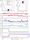 |
Fig. 1 Top panels (a1, a2) show the orbit of VEX on 5 November 2011 in cylindrical coordinates X and |
![Mathematical equation: $\[\sqrt{\mathrm{Y}^{2}+\mathrm{Z}^{2}}\]$](/articles/aa/full_html/2026/02/aa55227-25/aa55227-25-eq12.png)
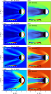 |
Fig. 2 Temporal evolution of magnetic field strength and plasma flow speed in the X–Z plane at four selected times (38.0, 39.0, 41.0, and 42.0 min). Each row corresponds to a specific time point, with the left and right columns showing magnetic field strength (a) and plasma flow speed (b), respectively. |
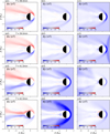 |
Fig. 3 Temporal evolution of the magnetic field components Bx, By and Bz in the X–Z plane before (38.0 and 39.0 min) and after (41.0 and 42.0 min) the ICME arrival. Each row represents a time snapshot, while columns (a), (b), and (c) correspond to Bx, By, and Bz, respectively. |
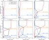 |
Fig. 4 Altitude profiles of pressures along the Venus–Sun line at 30, 38, 39, 41, 42, 158 min of simulation (ICME shock arrives Venus at 39 min). The blue, red, and black lines represent magnetic pressure, dynamic pressure and thermal pressure, respectively. The BS and IMB locations are indicated by orange and light blue dashed lines, respectively. |
Comparisons of the status of solar wind plasma and IMF and the Venusian magnetosphere before, during and after the ICME.
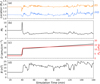 |
Fig. 5 (a) Temporal evolution of the locations of subsolar BS (orange line) and IMB (blue line). The corresponding upstream conditions are shown in the panels below, including (b) fast magnetosonic Mach number (black line), (c) solar wind density (black line) and dynamic pressure (red line), and (d) IMF strength (black line). |
3.2 Ionospheric variation
Besides the magnetosphere, the Venusian ionosphere can also be significantly affected by ICME, leading to shifts in the ionopause location and an enhancement of heavy ion fluxes near and above the ionopause region (Rout et al. 2024). In Figure 6, we compare the number density of ions and the magnetic field along the subsolar line at simulation times similar to Figure 4. Figure 6a1 presents a profile of the number densities of ion species and electrons from 100 to 500 km altitude under typical quiet solar wind conditions. Above 400 km altitude, the ionosphere is mainly dominated by H+, while lower regions are composed of three ions: O+, ![Mathematical equation: $\[\mathrm{O}_{2}^{+}\]$](/articles/aa/full_html/2026/02/aa55227-25/aa55227-25-eq20.png) , and
, and ![Mathematical equation: $\[\mathrm{CO}_{2}^{+}\]$](/articles/aa/full_html/2026/02/aa55227-25/aa55227-25-eq21.png) . The peak densities at 130 km are 6 × 105 cm−3 for
. The peak densities at 130 km are 6 × 105 cm−3 for ![Mathematical equation: $\[\mathrm{O}_{2}^{+}\]$](/articles/aa/full_html/2026/02/aa55227-25/aa55227-25-eq22.png) and 104 cm−3 for
and 104 cm−3 for ![Mathematical equation: $\[\mathrm{CO}_{2}^{+}\]$](/articles/aa/full_html/2026/02/aa55227-25/aa55227-25-eq23.png) . O+ dominates the ionosphere between 200 km and 350 km, and reaches the peak of 6 × 104 cm−3 at 210 km. The simulated ionosphere density is consistent with previous observations (Brace & Kliore 1991; Miller et al. 1984) and simulations (Ma et al. 2013). The ionopause is located at an altitude of 300–350 km, which is in good agreement with the mean observational altitudes of ~320 km to ~370 km (Knudsen & Miller 1992; Phillips et al. 1988). Figure 6a2 shows the altitude profile of the three components of the induced magnetic field. During the quiet period, the magnetic field stabilizes in a steady state.
. O+ dominates the ionosphere between 200 km and 350 km, and reaches the peak of 6 × 104 cm−3 at 210 km. The simulated ionosphere density is consistent with previous observations (Brace & Kliore 1991; Miller et al. 1984) and simulations (Ma et al. 2013). The ionopause is located at an altitude of 300–350 km, which is in good agreement with the mean observational altitudes of ~320 km to ~370 km (Knudsen & Miller 1992; Phillips et al. 1988). Figure 6a2 shows the altitude profile of the three components of the induced magnetic field. During the quiet period, the magnetic field stabilizes in a steady state.
At 38 minutes, the ion density and magnetic field profiles show slight changes. The dashed lines represent the distribution of corresponding parameters at 30 minutes, and remain consistent across all plots. At 39 minutes, the ICME shock reaches Venus, and Figure 6c1 clearly shows the ionosphere is compressed. The density of ![Mathematical equation: $\[\mathrm{CO}_{2}^{+}\]$](/articles/aa/full_html/2026/02/aa55227-25/aa55227-25-eq24.png) remains almost unchanged due to its photochemical equilibrium at low altitude ionosphere. Figure 6c2 shows that the induced magnetic field above 250 km altitude increases to over 100 nT, since the deeper penetration of the solar wind strengthens the magnetic barrier. Two minutes later, Figure 6d1 shows that the ionosphere is further compressed. In Figure 6d2, the magnetic field strength in the ionosphere increases. Under compression from the high solar wind dynamic pressure, the magnetic components By and Bz maintained high average values of 152 nT and 53 nT, respectively, between 180 and 300 km in altitude. While above 350 km, the rotation of the IMF under the ICME caused Bz to weaken and By to strengthen. Consequently, a steep gradient in both By and Bz develops across the 300–350 km transition layer. As the magnetosphere is compressed by high solar wind dynamic pressure, Bz and By keep high values between 180 and 300 km in altitude, averaging at 152 nT and 53 nT. As the IMF rotates under ICME, IMF Bz weakens and By strengthens over 350 km, causing a steep gradient in the By and Bz at 300–350 km. At 42 minutes when the enhanced IMF reaches Venus, the rotational influence of IMF extends to lower altitudes. The changes in magnetic topology and the descent of the transition altitude (from ~350 km to ~300 km) represent a simultaneous response to the increasing solar wind dynamic pressure of the ICME, which progressively compressed and lowered the ionopause.
remains almost unchanged due to its photochemical equilibrium at low altitude ionosphere. Figure 6c2 shows that the induced magnetic field above 250 km altitude increases to over 100 nT, since the deeper penetration of the solar wind strengthens the magnetic barrier. Two minutes later, Figure 6d1 shows that the ionosphere is further compressed. In Figure 6d2, the magnetic field strength in the ionosphere increases. Under compression from the high solar wind dynamic pressure, the magnetic components By and Bz maintained high average values of 152 nT and 53 nT, respectively, between 180 and 300 km in altitude. While above 350 km, the rotation of the IMF under the ICME caused Bz to weaken and By to strengthen. Consequently, a steep gradient in both By and Bz develops across the 300–350 km transition layer. As the magnetosphere is compressed by high solar wind dynamic pressure, Bz and By keep high values between 180 and 300 km in altitude, averaging at 152 nT and 53 nT. As the IMF rotates under ICME, IMF Bz weakens and By strengthens over 350 km, causing a steep gradient in the By and Bz at 300–350 km. At 42 minutes when the enhanced IMF reaches Venus, the rotational influence of IMF extends to lower altitudes. The changes in magnetic topology and the descent of the transition altitude (from ~350 km to ~300 km) represent a simultaneous response to the increasing solar wind dynamic pressure of the ICME, which progressively compressed and lowered the ionopause.
After the ICME shock passes through Venus, the solar wind dynamic pressure and density are gradually increasing. The peak of the induced magnetic field strength is enhanced from 160 nT at 42 minutes to 200 nT at 158 minutes, in response to the increase in solar wind dynamic pressure. VEX detected that the magnetic field strength at the outer boundary of the Venusian magnetic barrier could reach up to 250 nT during this event (Vech et al. 2015; Dimmock et al. 2018). Although our simulated peak (200 nT) is lower, this difference likely arises from uncertainties in the upstream solar wind conditions during the VEX measurement, which were not directly monitored as the spacecraft had already entered the magnetosphere. Therefore, our simulation still shows good agreement with observations. At 158 minutes, under the combined influence of the enhanced IMF and dynamic pressure, the compression of ionospheric ions is almost completely diminished. ![Mathematical equation: $\[\mathrm{CO}_{2}^{+}\]$](/articles/aa/full_html/2026/02/aa55227-25/aa55227-25-eq27.png) density generally keeps unchanged during whole simulation due to the photochemical control.
density generally keeps unchanged during whole simulation due to the photochemical control. ![Mathematical equation: $\[\mathrm{O}_{2}^{+}\]$](/articles/aa/full_html/2026/02/aa55227-25/aa55227-25-eq28.png) gradually returns to a distribution similar to that during the quiet period, and later it expands outward. As Figure 6f1 shows, a high density of
gradually returns to a distribution similar to that during the quiet period, and later it expands outward. As Figure 6f1 shows, a high density of ![Mathematical equation: $\[\mathrm{O}_{2}^{+}\]$](/articles/aa/full_html/2026/02/aa55227-25/aa55227-25-eq29.png) appears between 300 and 350 km. Meanwhile, the distribution of O+ approaches that during the quiet period. The ionospheric magnetic field undergoes highly complex variations in response to the drastically changing IMF in Figure 6f2. The Bz component experiences reversal at 190 km.
appears between 300 and 350 km. Meanwhile, the distribution of O+ approaches that during the quiet period. The ionospheric magnetic field undergoes highly complex variations in response to the drastically changing IMF in Figure 6f2. The Bz component experiences reversal at 190 km.
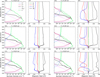 |
Fig. 6 Altitude profiles of number density and magnetic field within the ionosphere along the subsolar line at 30, 38, 39, 41, 42, and 158 min of simulation. Figures a1, b1, c1, d1, e1, f1 show the altitude profiles of number densities of different ion species and electrons: H+ (blue), O+ (red), |
![Mathematical equation: $\[\mathrm{O}_{2}^{+}\]$](/articles/aa/full_html/2026/02/aa55227-25/aa55227-25-eq25.png)
![Mathematical equation: $\[\mathrm{CO}_{2}^{+}\]$](/articles/aa/full_html/2026/02/aa55227-25/aa55227-25-eq26.png)
3.3 ICME impact on ion escape
Due to Venusian deuterium/hydrogen (D/H) ratio being about 100 times higher than that of Earth, Venus is widely believed to have had large amounts of water in its early history, possibly enough to form oceans (Donahue et al. 1982). Observations, however, reveal that the Venusian atmosphere is now extremely dry and harsh. Therefore, understanding how water in Venusian atmosphere was lost has become an important topic in planetary science. Atmospheric loss on Venus is suggested to be significantly dependent on the solar wind (Masunaga et al. 2019; Luhmann & Bauer 1992; Futaana et al. 2017). As severe space weather, ICME could increase greatly the ion escape, possibly accelerating the water loss on Venus (Edberg et al. 2011; Luhmann et al. 2007; Futaana et al. 2008). Here we quantitatively analyzed the effect of a realistic ICME on global ion escape from Venus, utilizing simulations. We assumed that the ions’ escape rate is entirely attributed to the outflow from this magnetotail plane. In order to estimate ion escape rates accurately, the loss flux of each ion species was integrated on a Y–Z plane where X = −2 RV in the magnetotail. The cells on this plane are cross sections of the grids intersected by the plane, with the values of physical quantities within the cells interpolated from the corresponding grid values and those of surrounding grids. Hence, the escape rate (ER) could easily be calculated:
![Mathematical equation: $\[E R_i=\sum_{\mathrm{X}=-2 R_V} D_i \cdot v_{x, i} \cdot A\]$](/articles/aa/full_html/2026/02/aa55227-25/aa55227-25-eq30.png) (6)
(6)
where Di represents the number density of ion species i, vx,i is velocity in X direction, and A denotes the cross sectional area of the grid through plane X = −2 RV.
Figure 7a shows the variation in the integrated escape rates of O+, ![Mathematical equation: $\[\mathrm{O}_{2}^{+}\]$](/articles/aa/full_html/2026/02/aa55227-25/aa55227-25-eq35.png) , and
, and ![Mathematical equation: $\[\mathrm{CO}_{2}^{+}\]$](/articles/aa/full_html/2026/02/aa55227-25/aa55227-25-eq36.png) , represented by the blue, red, and green lines, respectively. The y-axis is displayed on a logarithmic scale. Figures 7b and c show the upstream driving conditions of simulation: the IMF components By and Bz, as well as solar wind plasma density and velocity. To investigate the effect of the ICME on the escape rate, a simulation was conducted as a comparison in which driving conditions remain constant during quiet period. Since the first 40 minutes were used for initialization (and thus had less physical significance), we present escape data deemed reliable from 35 to 160 minutes. During the quiet period, the escape rates of
, represented by the blue, red, and green lines, respectively. The y-axis is displayed on a logarithmic scale. Figures 7b and c show the upstream driving conditions of simulation: the IMF components By and Bz, as well as solar wind plasma density and velocity. To investigate the effect of the ICME on the escape rate, a simulation was conducted as a comparison in which driving conditions remain constant during quiet period. Since the first 40 minutes were used for initialization (and thus had less physical significance), we present escape data deemed reliable from 35 to 160 minutes. During the quiet period, the escape rates of ![Mathematical equation: $\[\mathrm{O}_{2}^{+}\]$](/articles/aa/full_html/2026/02/aa55227-25/aa55227-25-eq37.png) and
and ![Mathematical equation: $\[\mathrm{CO}_{2}^{+}\]$](/articles/aa/full_html/2026/02/aa55227-25/aa55227-25-eq38.png) are on the order of 1023 s−1, with
are on the order of 1023 s−1, with ![Mathematical equation: $\[\mathrm{CO}_{2}^{+}\]$](/articles/aa/full_html/2026/02/aa55227-25/aa55227-25-eq39.png) exhibiting an escape rate of around 4.0 × 10²³ s−1 and
exhibiting an escape rate of around 4.0 × 10²³ s−1 and ![Mathematical equation: $\[\mathrm{O}_{2}^{+}\]$](/articles/aa/full_html/2026/02/aa55227-25/aa55227-25-eq40.png) around 6.0 × 10²³ s−1. As is indicated by the dashed lines, the rates of
around 6.0 × 10²³ s−1. As is indicated by the dashed lines, the rates of ![Mathematical equation: $\[\mathrm{O}_{2}^{+}\]$](/articles/aa/full_html/2026/02/aa55227-25/aa55227-25-eq41.png) and
and ![Mathematical equation: $\[\mathrm{CO}_{2}^{+}\]$](/articles/aa/full_html/2026/02/aa55227-25/aa55227-25-eq42.png) remain constant under quiet solar wind conditions. During ICME, the responses of the
remain constant under quiet solar wind conditions. During ICME, the responses of the ![Mathematical equation: $\[\mathrm{O}_{2}^{+}\]$](/articles/aa/full_html/2026/02/aa55227-25/aa55227-25-eq43.png) and
and ![Mathematical equation: $\[\mathrm{CO}_{2}^{+}\]$](/articles/aa/full_html/2026/02/aa55227-25/aa55227-25-eq44.png) are different. As is shown in the ion density profiles in Figure 6,
are different. As is shown in the ion density profiles in Figure 6, ![Mathematical equation: $\[\mathrm{CO}_{2}^{+}\]$](/articles/aa/full_html/2026/02/aa55227-25/aa55227-25-eq45.png) is concentrated at relatively low altitudes and exist in photochemical equilibrium, while
is concentrated at relatively low altitudes and exist in photochemical equilibrium, while ![Mathematical equation: $\[\mathrm{O}_{2}^{+}\]$](/articles/aa/full_html/2026/02/aa55227-25/aa55227-25-eq46.png) is affected by ICME. Thus,
is affected by ICME. Thus, ![Mathematical equation: $\[\mathrm{CO}_{2}^{+}\]$](/articles/aa/full_html/2026/02/aa55227-25/aa55227-25-eq47.png) escape rate stabilizes at around 6.0 × 10²³ s−1.
escape rate stabilizes at around 6.0 × 10²³ s−1. ![Mathematical equation: $\[\mathrm{O}_{2}^{+}\]$](/articles/aa/full_html/2026/02/aa55227-25/aa55227-25-eq48.png) escape rate shows more complex variation, finally maintaining an average level of 1.0 × 1024 s−1. O+ shows an escape rate of 6.0 × 1024 s−1, significantly higher than the other two ion species. Under typical solar wind driving, the O+ escape rate remains steady at approximately 9.0 × 1024 s−1 after initialization. During the ICME period, the O+ escape rate gradually increases from 1024 s−1 to 1025 s−1, eventually reaching 3.1 × 1025 s−1, which is over three times that of the comparison case. The result aligns with previous calculations based on observations (McComas et al. 1986; Barabash et al. 2007b; Masunaga et al. 2011; Jarvinen et al. 2009). The increased O+ escape is interpreted as a consequence of the elevated solar wind dynamic pressure, which drove a more efficient loss of O+ via the magnetotail on large timescales. Additionally, the escape rate exhibits notable perturbations, particularly around the 70 and 120 minute marks, which were likely caused by the dramatic variations in By and Bz, as is shown in Figures 7a and b.
escape rate shows more complex variation, finally maintaining an average level of 1.0 × 1024 s−1. O+ shows an escape rate of 6.0 × 1024 s−1, significantly higher than the other two ion species. Under typical solar wind driving, the O+ escape rate remains steady at approximately 9.0 × 1024 s−1 after initialization. During the ICME period, the O+ escape rate gradually increases from 1024 s−1 to 1025 s−1, eventually reaching 3.1 × 1025 s−1, which is over three times that of the comparison case. The result aligns with previous calculations based on observations (McComas et al. 1986; Barabash et al. 2007b; Masunaga et al. 2011; Jarvinen et al. 2009). The increased O+ escape is interpreted as a consequence of the elevated solar wind dynamic pressure, which drove a more efficient loss of O+ via the magnetotail on large timescales. Additionally, the escape rate exhibits notable perturbations, particularly around the 70 and 120 minute marks, which were likely caused by the dramatic variations in By and Bz, as is shown in Figures 7a and b.
In this simulation of a realistic event, we quantitatively determined that the O+ loss rate from Venus increases by a factor of 3 under an ICME. However, the significant variability of the driving conditions of the ICME introduces complexity and instability, causing a limited understanding of relative contribution of the dynamic pressure and IMF to the O+ loss rate. Edberg et al. (2011) emphasized the crucial role of solar wind dynamic pressure and IMF direction in increasing the escape rate during ICME and CIR events, specifically discussing them from observations. Due to observational constraints, the analysis is insufficiently quantitative. Therefore, we conducted three idealized simulation cases to explore quantitatively how the IMF and dynamic pressure respectively affect the O+ escape. Figure 8 illustrates the variations in O+ escape under four idealized solar wind inputs: the blue line corresponds to the input with both dynamic pressure pulse and IMF enhancement, the red line only dynamic pressure pulses, the green curve only IMF enhancement, and the black line as a control during quiet periods. The three simulations with more extreme upstream conditions ultimately result in escape fluxes higher than those during the quiet period. The O+ escape driven by the idealized ICME shows the greatest increase, reaching 4.0 × 1025 s−1. Comparing the red, cyan, and black lines, it is demonstrated clearly that either high solar wind dynamic pressure or an enhanced IMF strength alone can accelerate O+ escape. The red curve is significantly higher than the cyan curve, suggesting that high dynamic pressure has a more pronounced effect on enhancing the O+ escape flux compared to a strong IMF.
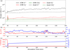 |
Fig. 7 Temporal variations in (a) the escape rates in heavy ions and (b, c) the corresponding upstream solar wind plasma and IMF conditions. Panel (a) shows the escape rates of O+ (black), |
![Mathematical equation: $\[\mathrm{O}_{2}^{+}\]$](/articles/aa/full_html/2026/02/aa55227-25/aa55227-25-eq31.png)
![Mathematical equation: $\[\mathrm{CO}_{2}^{+}\]$](/articles/aa/full_html/2026/02/aa55227-25/aa55227-25-eq32.png)
![Mathematical equation: $\[\mathrm{O}_{2}^{+}\]$](/articles/aa/full_html/2026/02/aa55227-25/aa55227-25-eq33.png)
![Mathematical equation: $\[\mathrm{CO}_{2}^{+}\]$](/articles/aa/full_html/2026/02/aa55227-25/aa55227-25-eq34.png)
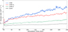 |
Fig. 8 Temporal variations in the O+ escape rate under different solar wind plasma and IMF conditions. The blue, red, green, and black lines represent simulations with realistic ICME driving, with high dynamic pressure pulses of solar wind only, with enhanced IMF only, and quiet conditions, respectively. |
4 Summary and discussion
In this study, we established a 120 min ICME driving condition to simulate the Venusian response to the ICME event on 5 November 2011. The simulation utilizes upstream IMF conditions of an ICME event detected by VEX, which was characterized by a significant intensification of upstream conditions. Specifically, the solar wind density increases from 10 cm−3 to 19 cm−3, and the velocity exhibits a sharp jump from approximately 400 km/s to 680 km/s upon the ICME’s arrival. This combined effect resulted in a peak solar wind dynamic pressure that is 5.8 times the pre-ICME value. Concurrently, IMF strength is intensified significantly, increasing from 8.68 nT to over 20 nT – a factor of 1.9 – and exhibits a clear rotation. By incorporating these realistic, time-varying conditions, the global simulation with high-order numerical algorithms allows us to examine systematically and quantitatively the detailed and fine variation of the Venusian plasma system. The results show rapid responses to the time-varying driving condition, with a compressed MI system and significantly accelerated heavy ion escape. Due to intense solar wind disturbances, the ICME impact causes complex effects on Venus MI system, which are not monotonous over time.
Model results show that the ICME shock significantly impacts the magnetosphere and ionosphere of Venus, with higher temperatures, denser plasma, faster flow, and enhanced IMF. Venus responds to the shock rapidly on a timescale of minutes, reaching a quasistable state after a brief period of instability. This rapid adaptation is evidenced by an average response time of 8.5 minutes to the IMF direction change (Slavin et al. 2009). The magnetic field strength in the dayside magnetosphere significantly increases, while the magnetotail is compressed. The plasma flow in the flank region accelerates beyond solar wind, which is also shown in the simulation of the Martian response to ICME (Ma et al. 2017). During the ICME event, the locations of plasma boundaries along the Venus-Sun line vary continuously. The results highlight that the Mf controls the BS location during the ICME. Also, the plasma boundary location exhibits a different response to increased dynamic pressure and enhanced IMF during ICME event. Ionospheric ion distributions experience compression upon the arrival of ICME, with a gradual weakening over time. The magnetic field within ionosphere exhibits highly complex variations due to the dramatically varying IMF. Regarding the identification of plasma boundary, while their absolute locations may vary depending on the specific method used, the primary conclusions of this study – concerning ICME-induced changes – rely on relative variation. A detailed comparison of different BS location methods represents a valuable direction for future work.
As the most intense solar eruptive event, understanding how an ICME impacts the ion escape rate of Venus contributes significantly to our understanding of Venus’ atmospheric evolution. Unlike Mars, the nonthermal escape driven by solar wind plays a dominant role in Venus’ atmosphere loss (Dubinin et al. 2011; Futaana et al. 2017), with a very high escape velocity (10.4 km/s) that prevents ions and neutral particles from undergoing Jeans escape. Several studies have been conducted to utilize the data from PVO and VEX to estimate the heavy ion escape, resulting in a range from 1024 s−1 to 1026 s−1 (McComas et al. 1986; Brace et al. 1987; Knudsen & Miller 1992; Nordström et al. 2013; Lundin 2011). Under typical quiet solar wind, Masunaga et al. (2011) calculated statistically the total O+ escape rate of (5.8 ± 2.9) × 1024 s−1. Meanwhile, atmospheric escape at Venus varies with upstream conditions and increases by a factor of 1.9 on average during CIRs and ICMEs (Edberg et al. 2011). Other observations also agree with the enhancement of ion escape (Luhmann et al. 2007; Futaana et al. 2008). In this study, we calculated the escape rate of major ions, O+, ![Mathematical equation: $\[\mathrm{O}_{2}^{+}\]$](/articles/aa/full_html/2026/02/aa55227-25/aa55227-25-eq49.png) , and
, and ![Mathematical equation: $\[\mathrm{CO}_{2}^{+}\]$](/articles/aa/full_html/2026/02/aa55227-25/aa55227-25-eq50.png) , under the influence of ICME. Among these, the O+ escape rate shows the most notable alteration, increasing from 1024 s−1 to 1025 s−1, finally reaching approximately 3.1 × 1025 s−1. Throughout the simulation, the total O+ escape rate demonstrates a sustained increase on large timescales. The quantitative analysis helps us to understand the dependence of Venus’ atmospheric escape on the dynamic solar wind and suggests an intricate physical mechanism for ion escape under realistic space weather. Furthermore, to isolate individual contributions of solar wind dynamic pressure and IMF, we performed controlled simulations with idealized conditions. The results demonstrate that both high dynamic pressure and a strengthened IMF can enhance the O+ escape rate, with dynamic pressure playing the predominant role. Moreover, Dang et al. (2022) demonstrates the pressure and magnetic field of solar wind can modulate the Kelvin-Helmholtz instability behavior and the oxygen ion loss rate. The relevant work is interesting and of the utmost importance in explaining the differences in atmospheres among terrestrial planets. In this study, these rough and intuitive effects of dynamic pressure and IMF strength on O+ escape require a more detailed discussion to obtain further insights into the physical mechanisms.
, under the influence of ICME. Among these, the O+ escape rate shows the most notable alteration, increasing from 1024 s−1 to 1025 s−1, finally reaching approximately 3.1 × 1025 s−1. Throughout the simulation, the total O+ escape rate demonstrates a sustained increase on large timescales. The quantitative analysis helps us to understand the dependence of Venus’ atmospheric escape on the dynamic solar wind and suggests an intricate physical mechanism for ion escape under realistic space weather. Furthermore, to isolate individual contributions of solar wind dynamic pressure and IMF, we performed controlled simulations with idealized conditions. The results demonstrate that both high dynamic pressure and a strengthened IMF can enhance the O+ escape rate, with dynamic pressure playing the predominant role. Moreover, Dang et al. (2022) demonstrates the pressure and magnetic field of solar wind can modulate the Kelvin-Helmholtz instability behavior and the oxygen ion loss rate. The relevant work is interesting and of the utmost importance in explaining the differences in atmospheres among terrestrial planets. In this study, these rough and intuitive effects of dynamic pressure and IMF strength on O+ escape require a more detailed discussion to obtain further insights into the physical mechanisms.
As the Venusian magnetosphere is dominated by solar wind, it is crucial to address its response to realistic driving conditions to advance our understanding of the evolution of Venus. Due to unavailable plasma data, we established the reasonable idealized plasma parameters of ICME driving, which cannot be perfectly consistent with the ICME event. The sparsity of solar wind plasma data introduces uncertainty in the exact calculation of parameters such as the Mf. However, it is important to note that the fundamental physical mechanisms discussed in the research are not changed. Meanwhile, the relative changes and comparative trends reported in this study – such as the compression and expansion of boundaries in response to varying upstream conditions – are robust against such uncertainties, as they depend on the coherent variation of driving parameters rather than their absolute precision. For plasma parameters, using linearly varying curves to fit the long-term realistic changes can produce reasonable results and should not compromise the integrity of physics. On the other hand, the extreme lack of in situ observational data also makes further research on Venus challenging. Our research raises an urgent need for observations of plasma environment at Venus in the future.
The model used in this study assumes a spherically symmetric neutral atmosphere distribution, and the Hall term is neglected in MHD equations. As was mentioned in Section 2, the low ratio of the ion’s gyroradius to Venusian radius justifies neglecting the Hall effect in the macroscopic flow (Ledvina et al. 2008). This is valid even for the major heavy ions; our calculations show the gyroradii of O+, ![Mathematical equation: $\[\mathrm{O}_{2}^{+}\]$](/articles/aa/full_html/2026/02/aa55227-25/aa55227-25-eq51.png) , and CO+ in the dayside magnetosheath are merely ~339.4 km, ~678.4 km, and ~933.8 km, respectively, all negligible compared to the planetary radius of 6051.8 km. In the magnetotail, however, these values increase significantly to 2522.5 km (0.417 RV) for O+, 5326.0 km (0.880 RV) for
, and CO+ in the dayside magnetosheath are merely ~339.4 km, ~678.4 km, and ~933.8 km, respectively, all negligible compared to the planetary radius of 6051.8 km. In the magnetotail, however, these values increase significantly to 2522.5 km (0.417 RV) for O+, 5326.0 km (0.880 RV) for ![Mathematical equation: $\[\mathrm{O}_{2}^{+}\]$](/articles/aa/full_html/2026/02/aa55227-25/aa55227-25-eq52.png) , and 7339.0 km (1.212 RV) for
, and 7339.0 km (1.212 RV) for ![Mathematical equation: $\[\mathrm{CO}_{2}^{+}\]$](/articles/aa/full_html/2026/02/aa55227-25/aa55227-25-eq53.png) , where the weaker magnetic field allows gyroradii to reach scales comparable to the planetary radius. As a result, the simulation results give more symmetric responses in dayside, which might deviate from the asymmetric distributions from the VEX measurements (Zhang et al. 2010; Chai et al. 2015). Although Hall effects can influence asymmetric structures at Venus, they play a secondary role in the large-scale ICME-driven dynamics examined here, where global pressure balance and mass loading are the primary controls, and the fundamental physics illustrated in this study remain unchanged. We note that implementing Hall physics is an active focus of our ongoing model development. The current work establishes a robust large-scale baseline against which the effects of more sophisticated physical treatments can be systematically compared in future studies. Note that variations in the EUV associated with the solar eruption are also not considered in this work, though it is acknowledged that EUV flux significantly affects ion escape rates from Venus (Masunaga et al. 2019). Additionally, the MHD simulations ignore the kinetic processes, which could have an influence on the interaction between Venus and the solar wind. McEnulty et al. (2010) reported that ICMEs accelerated pickup ions to energies higher than typical levels, potentially affecting ion escape rate. The high-density, high-velocity, and high-temperature plasma carried by ICMEs may cause more ions to be picked up, thereby leading to the precipitation of more energy into atmospheric particles. This leads us to use a Hall MHD or hybrid model to illustrate kinetic-scale processes for the Venusian response to ICMEs.
, where the weaker magnetic field allows gyroradii to reach scales comparable to the planetary radius. As a result, the simulation results give more symmetric responses in dayside, which might deviate from the asymmetric distributions from the VEX measurements (Zhang et al. 2010; Chai et al. 2015). Although Hall effects can influence asymmetric structures at Venus, they play a secondary role in the large-scale ICME-driven dynamics examined here, where global pressure balance and mass loading are the primary controls, and the fundamental physics illustrated in this study remain unchanged. We note that implementing Hall physics is an active focus of our ongoing model development. The current work establishes a robust large-scale baseline against which the effects of more sophisticated physical treatments can be systematically compared in future studies. Note that variations in the EUV associated with the solar eruption are also not considered in this work, though it is acknowledged that EUV flux significantly affects ion escape rates from Venus (Masunaga et al. 2019). Additionally, the MHD simulations ignore the kinetic processes, which could have an influence on the interaction between Venus and the solar wind. McEnulty et al. (2010) reported that ICMEs accelerated pickup ions to energies higher than typical levels, potentially affecting ion escape rate. The high-density, high-velocity, and high-temperature plasma carried by ICMEs may cause more ions to be picked up, thereby leading to the precipitation of more energy into atmospheric particles. This leads us to use a Hall MHD or hybrid model to illustrate kinetic-scale processes for the Venusian response to ICMEs.
Acknowledgements
This work was supported by the National Natural Science Foundation of China (42241115), the Project of Stable Support for Youth Team in Basic Research Field, CAS (YSBR-018), and the pre-research project on Civil Aerospace Technologies No. D020105 funded by China’s National Space Administration. Binzheng Zhang was supported by the National Natural Science Foundation of China General Program (42374216) and the RGC General Research Fund (173008221, 17308723, and 17315222). The authors are grateful for support from the ISSI/ISSI-BJ workshop “Multi-Scale Magnetosphere–Ionosphere–Thermosphere Interaction”. The calculations were completed on the supercomputing system in the Hefei Advanced Computing Center. VEX magnetic field data are available in the ESA’s Planetary Science Archive (https://archives.esac.esa.int/psa/ftp/VENUS-EXPRESS/MAG/). The model outputs used to generate the figures for analysis presented in this paper are being preserved online (https://doi.org/10.5281/zenodo.15186474).
References
- Barabash, S., Fedorov, A., Sauvaud, J., et al. 2007a, Nature, 450, 650 [NASA ADS] [CrossRef] [Google Scholar]
- Barabash, S., Sauvaud, J.-A., Gunell, H., et al. 2007b, P&SS, 55, 1772 [Google Scholar]
- Brace, L., & Kliore, A. 1991, Space Sci. Rev., 55, 81 [NASA ADS] [CrossRef] [Google Scholar]
- Brace, L., Kasprzak, W., Taylor, H., et al. 1987, J. Geophys. Res. Space Phys., 92, 15 [CrossRef] [Google Scholar]
- Brambles, O., Lotko, W., Damiano, P., et al. 2010, J. Geophys. Res. Space Phys., 115 [Google Scholar]
- Burkholder, B., Chen, L.-J., Sarantos, M., et al. 2024, Geophys. Res. Lett., 51, e2024GL108311 [Google Scholar]
- Chai, L., Wan, W., Fraenz, M., et al. 2015, J. Geophys. Res. Space Phys., 120, 4446 [Google Scholar]
- Chang, Q., Xu, X., Zhang, T., et al. 2018, ApJ, 867, 129 [Google Scholar]
- Chen, N., Lu, H., Cao, J., et al. 2025a, J. Geophys. Res: Planets, 130, e2024JE008401 [Google Scholar]
- Chen, N., Lu, H., Cao, J., et al. 2025b, J. Geophys. Res: Planets, 130, e2024JE008829 [Google Scholar]
- Collinson, G. A., Grebowsky, J., Sibeck, D. G., et al. 2015, J. Geophys. Res. Space Phys., 120, 3489 [CrossRef] [Google Scholar]
- Dang, T., Lei, J., Zhang, B., et al. 2022, Geophys. Res. Lett., 49, e2021GL096961 [Google Scholar]
- Dang, T., Zhang, B., Yan, M., et al. 2023, ApJ, 945, 91 [NASA ADS] [CrossRef] [Google Scholar]
- Dang, T., Lei, J., Zhang, B., et al. 2025, Geophys. Res. Lett., 52, e2025GL116892 [Google Scholar]
- Dimmock, A. P., Alho, M., Kallio, E., et al. 2018, J. Geophys. Res. Space Phys., 123, 3580 [NASA ADS] [CrossRef] [Google Scholar]
- Donahue, T., Hoffman, J., Hodges Jr, R., & Watson, A. 1982, Science, 216, 630 [NASA ADS] [CrossRef] [Google Scholar]
- Donahue, T., & Russell, C. 1997, Venus II: Geology, Geophysics, Atmosphere, and Solar Wind Environment, 3 [Google Scholar]
- Dong, C., Ma, Y., Bougher, S. W., et al. 2015, Geophys. Res. Lett., 42, 9103 [NASA ADS] [CrossRef] [Google Scholar]
- Dubinin, E., Fraenz, M., Fedorov, A., et al. 2011, Space Sci. Rev., 162, 173 [Google Scholar]
- Edberg, N. J., Lester, M., Cowley, S., et al. 2010, J. Geophys. Res. Space Phys., 115 [Google Scholar]
- Edberg, N. J., Nilsson, H., Futaana, Y., et al. 2011, J. Geophys. Res. Space Phys., 116 [Google Scholar]
- Fox, J. L., & Sung, K. 2001, J. Geophys. Res. Space Phys., 106, 21305 [NASA ADS] [CrossRef] [Google Scholar]
- Futaana, Y., Barabash, S., Yamauchi, M., et al. 2008, P&SS, 56, 873 [Google Scholar]
- Futaana, Y., Stenberg Wieser, G., Barabash, S., & Luhmann, J. G. 2017, Space Sci. Rev., 212, 1453 [NASA ADS] [CrossRef] [Google Scholar]
- Gillmann, C., Way, M. J., Avice, G., et al. 2022, Space Sci. Rev., 218, 56 [NASA ADS] [CrossRef] [Google Scholar]
- Hudson, M. K., Elkington, S. R., Li, Z., et al. 2021, Space Weather, 19, e2021SW002882 [Google Scholar]
- Jarvinen, R., Kallio, E., Janhunen, P., et al. 2009, Ann. Geophys., 27, 4333 [Google Scholar]
- Knudsen, W. C. 1988, J. Geophys. Res. Space Phys., 93, 8756 [Google Scholar]
- Knudsen, W. C., & Miller, K. L. 1992, J. Geophys. Res. Space Phys., 97, 17165 [Google Scholar]
- Ledvina, S., Ma, Y.-J., & Kallio, E. 2008, Space Sci. Rev., 139, 143 [Google Scholar]
- Luhmann, J. 1986, Space Sci. Rev., 44, 241 [NASA ADS] [CrossRef] [Google Scholar]
- Luhmann, J., & Bauer, S. 1992, Geophysical Monograph, 66 [Google Scholar]
- Luhmann, J., Kasprzak, W., & Russell, C. 2007, J. Geophys. Res: Planets, 112 [Google Scholar]
- Lundin, R. 2011, Space Sci. Rev., 162, 309 [NASA ADS] [CrossRef] [Google Scholar]
- Ma, Y., Nagy, A., Russell, C., et al. 2013, J. Geophys. Res. Space Phys., 118, 321 [NASA ADS] [CrossRef] [Google Scholar]
- Ma, Y., Russell, C., Fang, X., et al. 2017, J. Geophys. Res. Space Phys., 122, 1714 [CrossRef] [Google Scholar]
- Masunaga, K., Futaana, Y., Yamauchi, M., et al. 2011, J. Geophys. Res. Space Phys., 116 [Google Scholar]
- Masunaga, K., Futaana, Y., Persson, M., et al. 2019, Icarus, 321, 379 [NASA ADS] [CrossRef] [Google Scholar]
- McComas, D. J., Spence, H. E., Russell, C., & Saunders, M. 1986, J. Geophys. Res. Space Phys., 91, 7939 [CrossRef] [Google Scholar]
- McEnulty, T., Luhmann, J., de Pater, I., et al. 2010, P&SS, 58, 1784 [Google Scholar]
- Miller, K. L., Knudsen, W. C., & Spenner, K. 1984, Icarus, 57, 386 [Google Scholar]
- Nagy, A., Cravens, T., Smith, S., Taylor Jr, H., & Brinton, H. 1980, J. Geophys. Res. Space Phys., 85, 7795 [Google Scholar]
- Nordström, T., Stenberg, G., Nilsson, H., Barabash, S., & Zhang, T. 2013, J. Geophys. Res. Space Phys., 118, 3592 [Google Scholar]
- Phillips, J., & Russell, C. 1987, J. Geophys. Res. Space Phys., 92, 2253 [CrossRef] [Google Scholar]
- Phillips, J., Luhmann, J., Knudsen, W., & Brace, L. 1988, J. Geophys. Res. Space Phys., 93, 3927 [Google Scholar]
- Ribas, I., Guinan, E. F., Güdel, M., & Audard, M. 2005, ApJ, 622, 680 [Google Scholar]
- Rong, Z., Barabash, S., Futaana, Y., et al. 2014, J. Geophys. Res. Space Phys., 119, 8838 [NASA ADS] [CrossRef] [Google Scholar]
- Rout, D., Thampi, S. V., Miyoshi, Y., Pant, T. K., & Bhardwaj, A. 2024, J. Geophys. Res. Space Phys., 129, e2024JA032553 [Google Scholar]
- Russell, C., Chou, E., Luhmann, J., et al. 1988, J. Geophys. Res. Space Phys., 93, 5461 [Google Scholar]
- Russell, C., Luhmann, J., & Strangeway, R. 2006, P&SS, 54, 1482 [Google Scholar]
- Slavin, J. A., Acuña, M. H., Anderson, B. J., et al. 2009, Geophys. Res. Lett., 36 [Google Scholar]
- Vech, D., Szego, K., Opitz, A., et al. 2015, J. Geophys. Res. Space Phys., 120, 4613 [CrossRef] [Google Scholar]
- Way, M. J., Del Genio, A. D., Kiang, N. Y., et al. 2016, Geophys. Res. Lett., 43, 8376 [NASA ADS] [CrossRef] [Google Scholar]
- Wood, B. E., Müller, H.-R., Zank, G. P., Linsky, J. L., & Redfield, S. 2005, ApJ, 628, L143 [NASA ADS] [CrossRef] [Google Scholar]
- Xu, Q., Xu, X., Chang, Q., et al. 2019, ApJ, 876, 84 [Google Scholar]
- Xu, Q., Xu, X., Zhang, T., et al. 2021, A&A, 652, A113 [NASA ADS] [CrossRef] [EDP Sciences] [Google Scholar]
- Zhang, T., Luhmann, J., & Russell, C. 1991, J. Geophys. Res. Space Phys., 96, 11145 [NASA ADS] [CrossRef] [Google Scholar]
- Zhang, T., Khurana, K., Russell, C., et al. 2004, ASR, 33, 1920 [Google Scholar]
- Zhang, T., Delva, M., Baumjohann, W., et al. 2008, P&SS, 56, 790 [Google Scholar]
- Zhang, T., Baumjohann, W., Du, J., et al. 2010, Geophys. Res. Lett., 37 [Google Scholar]
- Zhang, B., Sorathia, K. A., Lyon, J. G., et al. 2019, ApJS, 244, 20 [NASA ADS] [CrossRef] [Google Scholar]
- Zhao, J., Lu, H., Cao, J., et al. 2025, A&A, 694, A220 [NASA ADS] [CrossRef] [EDP Sciences] [Google Scholar]
All Tables
Comparisons of the status of solar wind plasma and IMF and the Venusian magnetosphere before, during and after the ICME.
All Figures
|
Fig. 1 Top panels (a1, a2) show the orbit of VEX on 5 November 2011 in cylindrical coordinates X and |
| In the text | |
|
Fig. 2 Temporal evolution of magnetic field strength and plasma flow speed in the X–Z plane at four selected times (38.0, 39.0, 41.0, and 42.0 min). Each row corresponds to a specific time point, with the left and right columns showing magnetic field strength (a) and plasma flow speed (b), respectively. |
| In the text | |
|
Fig. 3 Temporal evolution of the magnetic field components Bx, By and Bz in the X–Z plane before (38.0 and 39.0 min) and after (41.0 and 42.0 min) the ICME arrival. Each row represents a time snapshot, while columns (a), (b), and (c) correspond to Bx, By, and Bz, respectively. |
| In the text | |
|
Fig. 4 Altitude profiles of pressures along the Venus–Sun line at 30, 38, 39, 41, 42, 158 min of simulation (ICME shock arrives Venus at 39 min). The blue, red, and black lines represent magnetic pressure, dynamic pressure and thermal pressure, respectively. The BS and IMB locations are indicated by orange and light blue dashed lines, respectively. |
| In the text | |
|
Fig. 5 (a) Temporal evolution of the locations of subsolar BS (orange line) and IMB (blue line). The corresponding upstream conditions are shown in the panels below, including (b) fast magnetosonic Mach number (black line), (c) solar wind density (black line) and dynamic pressure (red line), and (d) IMF strength (black line). |
| In the text | |
|
Fig. 6 Altitude profiles of number density and magnetic field within the ionosphere along the subsolar line at 30, 38, 39, 41, 42, and 158 min of simulation. Figures a1, b1, c1, d1, e1, f1 show the altitude profiles of number densities of different ion species and electrons: H+ (blue), O+ (red), |
| In the text | |
|
Fig. 7 Temporal variations in (a) the escape rates in heavy ions and (b, c) the corresponding upstream solar wind plasma and IMF conditions. Panel (a) shows the escape rates of O+ (black), |
| In the text | |
|
Fig. 8 Temporal variations in the O+ escape rate under different solar wind plasma and IMF conditions. The blue, red, green, and black lines represent simulations with realistic ICME driving, with high dynamic pressure pulses of solar wind only, with enhanced IMF only, and quiet conditions, respectively. |
| In the text | |
Current usage metrics show cumulative count of Article Views (full-text article views including HTML views, PDF and ePub downloads, according to the available data) and Abstracts Views on Vision4Press platform.
Data correspond to usage on the plateform after 2015. The current usage metrics is available 48-96 hours after online publication and is updated daily on week days.
Initial download of the metrics may take a while.