| Issue |
A&A
Volume 706, February 2026
|
|
|---|---|---|
| Article Number | A171 | |
| Number of page(s) | 12 | |
| Section | The Sun and the Heliosphere | |
| DOI | https://doi.org/10.1051/0004-6361/202555756 | |
| Published online | 09 February 2026 | |
A new method of deriving Doppler velocities for Solar Orbiter SPICE
1
Southwest Research Institute, 1301 Walnut St Suite 400 Boulder CO 80302, USA
2
UKRI STFC, RAL Space Didcot OX11 0QX, UK
3
Université Paris-Saclay, CNRS, Institut d’Astrophysique Spatiale Bâtiment 121 91405 Orsay, France
4
Department of Physics, Catholic University of America 620 Michigan Avenue Washington DC 20064, USA
5
Heliophysics Division Goddard Space Flight Center Greenbelt MD 20771, USA
6
ETH-Zürich Wolfgang-Pauli-Str. 27 8093 Zürich, Switzerland
7
Physikalisch-Meteorologische Observatorium Davos/World Radiation Center (PMOD/WRC) Dorfstrasse 33 7260 Davos Dorf, Switzerland
8
Aerospace Engineering Sciences, University of Colorado 3775 Discovery Drive Boulder CO, USA
★ Corresponding author: This email address is being protected from spambots. You need JavaScript enabled to view it.
Received:
31
May
2025
Accepted:
4
November
2025
Abstract
This paper presents a follow-up to previous work on correcting point-spread-function (PSF)-induced Doppler artifacts in observations by the SPICE spectrograph on Solar Orbiter. In a previous paper, we demonstrated the correction of these artifacts in the y − λ plane with PSF regularization, treating the forward problem with a method based on large sparse matrix inversion. It has since been found that similar apparent artifacts are also present in the x − λ direction, i.e., across adjacent slit positions. Correcting this is difficult (although not impossible) with the previous matrix inversion method due to the time variation between slit positions. We have therefore devised a new method that addresses both x − λ and y − λ artifacts simultaneously by applying wavelength-dependent shifts at each x − y plane of the spectral cube. This paper demonstrates the SPICE data issue, describes the new method, and shows a comparison with the previous one. We explore the time variation of the correction parameters for the SPICE data and show a clear orbit dependence. The results of the method are significantly higher-quality Doppler signals, which we estimate at less than ∼5 km/s uncertainty for brighter lines in the absence of other systematics. Furthermore, we show the new SPICE polar observation results as a demonstration. The correction codes are written in Python, publicly available on GitHub, and can be directly applied to SPICE level 2 datasets.
Key words: line: profiles / instrumentation: spectrographs / techniques: high angular resolution / techniques: imaging spectroscopy / Sun: abundances / Sun: corona
© The Authors 2026
 Open Access article, published by EDP Sciences, under the terms of the Creative Commons Attribution License (https://creativecommons.org/licenses/by/4.0), which permits unrestricted use, distribution, and reproduction in any medium, provided the original work is properly cited.
This article is published in open access under the Subscribe to Open model. This email address is being protected from spambots. You need JavaScript enabled to view it. to support open access publication.
1. Introduction
This paper is a follow-up on a previous publication on the correction of point spread function (PSF) artifacts in Solar Orbiter SPICE (Plowman et al. 2023, from now on Paper I), which contains a more detailed review of the problem. Nevertheless, we begin with an abbreviated review and update in this section.
The Spectral Imaging of the Coronal Environment (SPICE, Spice Consortium 2020; Fludra et al. 2021) is an EUV slit scanning spectrograph on board Solar Orbiter (Müller et al. 2020; García Marirrodriga et al. 2021). It is designed to distinguish between solar wind source models by inferring the elemental composition of solar wind source regions on the surface of the Sun, while also detecting outflow velocities by means of the Doppler shifts in the atomic lines being observed (Zouganelis et al. 2020). SPICE was designed in synergy with the in situ Solar Wind Analyzer (SWA) suite of instruments on Solar Orbiter, to enable combined observations that trace the evolution of solar wind streams from the surface of the Sun to the Solar Orbiter spacecraft (Owen et al. 2020).
SPICE observes the solar spectrum in two wavelength windows, from 704 to 790 Å and from 973 to 1049 Å (Spice Consortium 2020). The spectral lines at these wavelengths are sensitive to solar plasma temperatures ranging from 10 kK to 1.0 MK, with the addition of two hotter Fe XVIII and Fe XX lines that can only be seen in flares (Young et al. 2025). These windows were chosen to maximize the selection of complementary (similar temperature sensitivity yet differing atomic ionization susceptibility) line pairs for measuring atomic abundance in the solar wind source regions (Varesano et al. 2024).
Although abundance measurements are the primary driver for SPICE, Doppler velocity measurements (i.e., fitting the profiles of the spectral lines in wavelength and thereby identifying the mean velocity of the emitting regions via the Doppler effect) are crucial for the maximal scientific output of the mission. It is a key piece of information in identifying solar wind source regions (Hassler et al. 1999; Harra et al. 2008), and such Doppler velocity measurements provide initial conditions for understanding the driving mechanisms and evolution of the solar wind (Baker et al. 2009). Additionally, accurately determining the properties of overlapping spectral lines (whether blended, or merely near each other in wavelength) is dependent on the spectral veracity of the data.
A further advantage of SPICE observations is that, in conjunction with Earth-perspective spectral observatories such as the Hinode EUV Imaging Spectrograph (EIS, Culhane et al. 2007) and the Interface Region Imaging Spectrograph (IRIS, De Pontieu et al. 2014), they can provide multi-viewpoint spectral and Doppler shift observations of solar features of interest. This is an entirely new capability offered by Solar Orbiter, and leveraging this capability requires well-calibrated Doppler shift observations.
Early in the Orbiter mission, it was found that SPICE Doppler velocity maps tend to show a pattern of elongated, overly large Doppler shifts around bright features (Fludra et al. 2021). An inspection of the spectra (see Figures 1 and 2) showed that an apparent tilted PSF feature in the y − λ plane is responsible. This causes light from bright features to leak into adjacent spatial pixels at offset wavelengths. To correct this issue, we developed a sparse matrix correction method, which works by effectively deconvolving (although by some definitions a deconvolution involves a spatially invariant kernel, whereas the sparse matrix method does not have this limitation) the PSF (Plowman et al. 2023). We then reapplied a nominal PSF, making it a PSF regularization approach (i.e., we first removed the aberrant PSF, then we reapplied the nominal PSF so that the resulting data would be free of noise and sharpening artifacts). The results of this procedure, as well as example PSF artifact lobes, are shown in Figure 1.
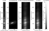 |
Fig. 1. Illustration of the SPICE PSF issue in the y − λ plane. The PSF is tilted in the y − λ plane as shown in panel (b), causing leakage of signal from bright features to adjacent pixels, not strictly at the same y or λ values, as shown in panels (c) and (d). Measurements of Doppler velocity from the data in panels (c) and (d) would lead to artificial Doppler shifts, as shown in Figure 2. |
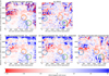 |
Fig. 2. Illustration of the Doppler velocity lobes caused by SPICE PSF artifacts during a co-observing campaign between IRIS and SPICE. The SPICE data show a characteristic redshift and blueshift pattern (examples circled) around bright intensity features – compare the top left panel (IRIS) with the top right panel (SPICE), both observing the same location. This pattern similarly appears in IRIS (not shown) when the PSF from Figure 1 is applied to IRIS (not shown) and (largely) disappears when the PSF regularization method described in Plowman et al. (2023) is applied. This is strong evidence that the Doppler velocity lobes are caused by the PSF tilt out of λ and into y. |
It was more recently discovered (Young, 2023, private communication) that an apparently similar issue aliases bright features into x (i.e., the slit scan direction, compared to the y-direction corresponding to the one along the slit) at differing λ locations. This was originally discovered by noticing that when a spectral cube sequence is sliced through the wavelength axis, an apparent image-wide shift is observed, as shown in Figure 3. This method of visualization is equivalent that of the y − λ image shown above, and the x − λ image can show a similar tilt to that in the y − λ image. It should be noted that the x-direction is constructed by rastering perpendicular to the slit direction by stepping from the primary mirror tilt, while only the y − λ plane is instantaneously imaged directly on the detector.
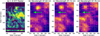 |
Fig. 3. Illustration of the x − λ and y − λ shifts in a slice of a SPICE spectral cube, with the intensity raster shown in the C III 977 Å line. Panels (b), (c), and (d) show zoomed-in slices (corresponding to the red square in panel (a)) where the x − y shift is apparent as a slight translation of the same features when scanning through consecutive wavelengths. Please see the online for an illustration of this effect. |
The presence of this kind of effect in x − λ images was not initially expected since it was thought that the presence of the slit would confine such spatial-spectral crosstalk to the slit plane. Additionally, some initially considered observations did not manifest a detectable x − λ shift or significant Doppler shift artifacts, which contributed to their being overlooked (we return to the temporal variation of these effects later in the paper). Nevertheless, since the behavior of the x − λ shift appears otherwise equivalent to that in the y − λ direction, we treat it – “to the same natural effects we must, as far as possible, assign the same causes” (Newton 1687) – as also being caused by the general PSF shape. Referring to the optical layout of SPICE (Figure 3 of Spice Consortium 2020), we note that the diffraction grating is downstream from the slit, so the slit ought to isolate the observations from grating-induced x − λ crosstalk. The mirror enclosure, containing the scanning mechanism, is upstream of the slit; therefore, this would seem to implicate the mirror as the source of this effect. It is not exactly clear what the physical mechanism is for this optical aberration at this point, although the mirror is subject to considerable thermal stress at perihelia. In any case, it is not the purpose of this paper to fully explain the effect but rather to show how it can be corrected, which we turn to next.
First, we consider the use of the previously developed method in Paper I. It was specifically built to permit multidimensional PSF correction, and it is in fact capable of doing so. However, two significant issues make it quite difficult to apply the full 3D PSF correction using this method:
-
It has proven quite challenging to find a sufficiently accurate PSF model applicable for different times during the mission. In principle, given perfect knowledge of the instrument, it could be calculated. However, we lack detailed information about the state of the instrument and a clear understanding of the origin of this optical aberration, which prevents us from predicting the instantaneous 3D instrumental PSF. Instead, we are left with an unknown time-varying 3D PSF that has a vastly larger parameter space to search than a 2D one. Additionally, the correction itself is much more computationally demanding in 3D than in 2D, so the compute time to search the 3D PSF space is orders of magnitude more than for the 2D PSF space.
-
Even if ignoring point 1, the x direction is obtained by rastering in time. This means that each x slice is at a different time than the others, and since the solar surface changes on temporal scales similar to the scanning time steps, the different raster steps are observing different solar sources. The forward matrix inversion or deconvolution-based schemes assume that the instrument observes the same source throughout the whole rastering process. Whenever that assumption is broken, the corrected image will exhibit large spikes as the algorithm attempts to describe a temporal jump with an incorrect PSF. This could be addressed by explicitly adding a fourth dimension – time – to the inversion. However, the data lacks sufficient information to fully disambiguate the temporal and spatial x directions, while again adding significant computational overhead.
Instead, we have found that a simpler method, based on corrective image shifts (or skews, depending on the axis of the spectral cube being viewed), can jointly address PSF artifacts in both the x − λ and the y − λ directions. Although this approach lacks the rigor, completeness, and spatial and spectral resolution improvements of the previous reconstruction method, it appears to reduce PSF artifacts as well as or better than the previous method. Moreover, it is far less computationally demanding and does not require prior knowledge of the exact instantaneous shape of the PSF. We now turn to describing and demonstrating this method.
2. Description of the new PSF correction method
Because the PSF tilt appears as a shift when scanning through wavelength (see panel (i) of Figure 4), we applied a compensating wavelength-dependent spatial shift to each x − y plane (constant wavelength plane) of the spectral cube. For example, if each pixel of an x − y plane in the input cube at wavelength λk lay at coordinates (xi, yj), we re-interpolated the output cube to new pixel coordinates (xi′,yj′) given by
 (1)
(1)
After testing, we found that a linear function for the shifts per unit wavelength (fx(λk),fy(λk)) from wavelengths λk suffices:
 (2)
(2)
where λ0 is a reference wavelength (usually the center of the spectral window or reference wavelength for the line in question) and Δx, Δy are the constant coefficients of the shifts. With this approach in place, counteracting the PSF effects on the Doppler shifts is a simple matter of re-interpolating the image to the new coordinates, producing the results in panel (ii) of Figure 4. We used the scipy.interpolate.RegularGridInterpolator method, which is a part of the scipy scientific Python programming package (Virtanen et al. 2020), for performing the skew correction. The default settings for the interpolation mode were used.
Wavelength-dependent shifting introduces (typically) sub-pixel spatial shifts in the image, depending on the wavelength of a spectral line at each pixel relative to the reference wavelength used for the correction. That is, if a spectral line in a particular spatial pixel is centered at wavelength Δλ relative to the reference wavelength, its image position shifts by ΔxΔλ and ΔyΔλ in x and y, respectively. This can be reversed after fitting the spectral lines by re-interpolating the fit found at each pixel, based on the line wavelength found by the fitting procedure. That is, after we applied the correction to the spectral cube, we performed a final spatial shift of −ΔxΔλ and ΔyΔλ for each spatial pixel. This nonhomogeneous “image-warping” (or “de-warping,” rather) interpolation step is shown in panel (iii) of Figure 4.
This approach has significant advantages over the previous method from Paper I, as described below:
-
This correction method can be executed very quickly (a matter of minutes on a single CPU on a modern computer for a single SPICE raster), making the computational overhead of applying the correction negligible compared to the other components of spectral line analysis (primarily the line fitting of the spectral profiles).
-
Unlike the PSF-deconvolution-like method, which is based on large sparse matrix inversions, this method has minimal susceptibility to time variation between raster positions – only a small temporal smoothing is introduced.
-
Due to the speed and simplicity of this method (only two parameters Δx and Δy need to be optimized), a brute force search for the optimum parameters is practical and achievable with minimal computational cost. We implemented and carried out such a search, described here in subsequent sections.
However, there are tradeoffs compared to the regularization approach from Paper I, which we consider modest relative to the advantages: First, this method does not enhance spatial resolution, unlike the PSF regularization from Paper I. On the contrary, the multiple layers of interpolation in the new method cause a spatial resolution decrease of up to about one pixel, roughly a factor of 1.5. Furthermore, de-warping (last step of the algorithm in Figure 4) incurs some computational overhead, although this is still negligible compared to the 3D PSF deconvolution problem. We implemented the correction algorithm, including the final de-warping re-interpolation step using the scipy.interpolate.LinearNDInterpolator method, with methods from numpy and scipy (Virtanen et al. 2020). The results obtained from the application of the new method to the SPICE level-2 dataset are shown in Figure 5. The resolution loss due to interpolation does not appear to be visually noticeable compared with the previous correction (see Figure 1). When equivalent correction parameters between the old and new correction methods are used (i.e., only considering y − λ correction), the results look extremely similar, as shown in the comparison between Figures 2 and 5. However, we found that applying both x and y shift corrections yields a result that matches that of IRIS even better.
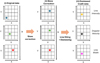 |
Fig. 4. Schematic of the algorithm. Left panels: Representation of the original data showing the wavelength-dependent spatial shift. The line center location is shown by the green star in the middle row. Middle panels: Representation of the data after the shift (or skew) is removed, showing that a leftover spatial shift is present – the line center position has moved compared to the input. Right panels: After line fitting, the deskewing moves the position of the fit parameter images back to the original line center position. |
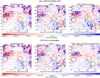 |
Fig. 5. New correction method applied to the same dataset as in Figure 2. Top row (panels (a)): Result from a y-only wavelength shift applied with the same parameters used in the aforementioned figure. Second row (panels (b)): Results with both x and y wavelength-dependent shifts. Notably, including only the y-shift shown in panels (a) does not fully remove the Doppler velocity artifacts. In contrast, including the full x − y shift results in very good agreement between the IRIS and SPICE observations. |
3. Estimation of correction parameters
To apply the aforementioned method to new SPICE data, the shift parameters Δx and Δy need to be determined. These parameters cannot be readily estimated from the known instrument configuration or calibration data, since neither provides sufficient information. Potentially, stellar observations may provide an occasional one-point check of PSF aberrations; however, these data are only taken occasionally. We presage subsequent parts of the paper (see Section 4) to note the significant time variation in this effect and a potential wavelength-dependent variation. Hence, an occasional calibration observation and the hand-tuned set of parameters used in the previous correction paper do not suffice. Instead, we propose an automated parameter search that produces good results.
In order to carry out an automated search for shift parameters, a figure of merit is required to quantify how well a given parameter set performs. We find that the standard variation of the Doppler shifts in the line fits (after applying the correction with a proposed set of parameters) produces a high-veracity figure of merit. The rationale for this is that the PSF aberration produces artificial apparent Doppler signals where the Sun exhibits none, but is quite unlikely to remove any existent ones. Consequently, we use this as the figure of merit in the shift parameter search. The search only includes pixels with estimated Doppler uncertainty (see Appendix A for uncertainty estimation) less than half the estimated Doppler shift, relative to the median wavelength after de-trending.
Before estimating the figure of merit for SPICE, we subtracted a planar trend from the Doppler shift across the entire image fit with a simple linear least-squares procedure. This is necessary because SPICE shows a significant trend in both x and y. This trend is significantly larger than the effects of solar rotation, which the above de-trending procedure also removes (although it is less accurate over large regions due to solar curvature and differential rotation). The resulting de-trended Doppler shift appears visually free of such trends, and we use it in the output example figures shown later in the paper (e.g., Figures 6 and 10). We are considering adding an explicit solar rotation to future versions of the code, which will result in higher-quality de-trended results for large fields of view.
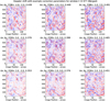 |
Fig. 6. De-trended Doppler shift signals, on which the figure of merit is based, for the SPICE observations used in the previous PSF work in Paper I and Figure 5. The subpanels show the resulting Doppler shifts from different shift parameters, noted above each subplot. With the highest quality Doppler shift correction around Δx = 2 arc second/Å and Δy = −2 arc second/Å this figure is consistent with the automated search determination of [2, −1.667], as shown in Figure 7. |
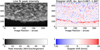 |
Fig. 10. Example polar observations with PSF corrections for data taken on March 23, 2025. The corrections allow high-quality Doppler shift measurements to be taken at the Sun’s poles – measurements never made before – as Solar Orbiter progresses to higher latitude orbits in later phases of its mission. |
To find the best correction parameter, we used a combination of brute force and an adaptive grid search. An initial grid of 5 × 5 points was laid out, covering the range of shift parameters from −5 to 5 arc seconds per Angstrom. These grid dimensions were chosen to cover the typical range of the parameters. We then checked each of the 25 parameters on the initial grid. Following this, we refined the results from this initial grid by starting with a higher-resolution 11 × 11 point grid covering the same range. We did not compute the figure of merit for all points on this grid, since we are only interested in the parameter space with the smallest figure of merit. Instead, we interpolated the results for the initial grid onto this new grid, then we computed the figure of merit for the 20 grid points with the lowest (interpolated) figure of merit. These will be focused on as the lowest point(s) of the merit function found so far. Finally, we repeated this refinement step with a 31 × 31 point grid, incorporating the points at both earlier grid spacings and computing the figure of merit for the most suitable 20 grid points. To demonstrate the performance of this search method and the proposed figure of merit, we show in Figure 6 the de-trended Doppler signals, which the figure of merit is based upon, for a grid of Δx and Δy parameters. The patterns in the Doppler shifts resulting from the different shift parameters (noted as the subplot titles) are clearly apparent, as are the characteristic blue and redshift signatures of the Doppler artifact for some correction parameters, such as those in the opposite direction of the required correction. The figure shows the full frame of the same data used for comparison with IRIS in Figures 2 and 5, which show a subfield in the upper left of Figure 6. For this dataset, the shift parameters of Δx = 2, Δy = −2 arc seconds per Å clearly indicate the smallest overall Doppler shifts as well as the best correspondence with IRIS, as shown in the previous figures. The parameter search figure of merit is the standard deviation of the Doppler shifts, shown in each of these panels. It should be noted that the plots suppress high-uncertainty pixels using a soft rolloff instead of the hard cut used to compute the figure of merit.
Figure 7 further illustrates the figure of merit surface as a function of Δx and Δy, as mapped out by the automated search algorithm. For the C III 977 Å observation shown in the left panel, used previously throughout the paper, we computed the figure of merit over the parameter shift space shown in the right panel. The iterative refinement search algorithm works as anticipated by the pattern of the points being sampled, and it is evident that the merit function surface is fairly smooth. The best parameter pair found is Δx = 2, Δy = −1.67, consistent with the previously shown results in Figure 6. We note that these parameters were also used for comparison with the IRIS data in Figure 5, producing excellent correspondence between the data from the different instruments.
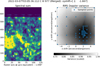 |
Fig. 7. Figure of merit surface in the x − λ and y − λ shift parameter for the SPICE observations obtained during the IRIS coordinated observing campaign used for the previous PSF estimation efforts. Right panel: Figure of merit surface. Left panel: Spectral sum of the window for comparison in the C III 977 Å line. The spectral sum is calculated at each pixel by summing the intensity across all wavelengths in the spectrum. The blue points in the right panel denote where the search procedure checked the figure of merit. The figure of merit shows a clear preference for both x − λ and y − λ shifts, as confirmed by the better match to IRIS observations. |
As previously mentioned, this result was derived without attempting to specifically tune the correction or the parameter search to recover the IRIS observations. The search algorithm only optimized the standard deviation of the de-trended Doppler shifts in SPICE, with no reference to the IRIS observations. The IRIS observation comparison was only carried out after the new algorithm had found its preferred candidate parameter pair. Therefore, the improved correspondence with the IRIS data, compared to the previous method or the y − λ only correction, itself validates the method.
To further validate this method, we applied the full correction stack to a set of synthetic observations. These observations had random Gaussian line amplitudes, Doppler shifts, and line widths, with some smoothing so that the overall intensity pattern resembled the small-scale chromospheric features observed in the cooler SPICE lines. To these observations, we applied a SPICE-like PSF with a nonzero angle in its orientation with respect to both the x − λ and y − λ planes, resulting in nonzero shifts in both x and y. We synthesized SPICE-equivalent data with this PSF, then searched for its parameters with our algorithm, producing line fits at the end. For a full apples-to-apples comparison, we produced another SPICE-equivalent dataset using a PSF with no x − λ or y − λ orientation, so that this dataset had no PSF-induced Doppler artifacts. The results of this “end-to-end” test are shown in Figure 8. We find that the residual differences between the corrected and no PSF aberration Doppler shift dataset features are less than 5 km/s, except in very low signal regions. This agreement is shown in the bottom left of Figure 8.
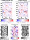 |
Fig. 8. Results of an “end-to-end” test of the new method using random test data. Top left: Doppler shifts with a nominal (no aberration) PSF. Top right: Doppler shifts with an aberrant PSF and correction, produced from the same underlying data. The correction recovers the test results well – at lower right the magnitude of the difference between the two is shown to be under 5 km/s except for very low signal regions adjacent to high signal ones. The uncorrected Doppler shifts (lower center) show far larger differences, overwhelming the actual signal in this test dataset. The line fit intensity is shown at the lower left for reference. |
4. Results and discussion
We described a new method to derive Doppler velocities and, more generally, to remove a persistent optical aberration in the data from the SolO/SPICE instrument. This new method removes the PSF artifacts in the data, while applying a skew correction to the SPICE spectral cubes. We tested the method on a synthetic dataset in an end-to-end instrumental fashion to demonstrate that it works as expected; the results are shown in Figure 8. Furthermore, comparing the results from our method on real SPICE data with corresponding IRIS observations, shown in Figure 2, illustrate that our method works as anticipated.
We must emphasize that this method can operate on data from time ranges when the SPICE PSF is not known a priori. Hence, an investigation of the time evolution of the shift parameters is warranted. We derived the shifts from our search algorithm for the SPROUTs dataset, which is a SPICE synoptic observing program (Varesano et al. 2025) – the acronym indicates that they are SynoPtic observations made OUT of coordinated Remote-sensing windows, i.e., they are not coordinated with the other instruments which makes them easy to recurrently schedule when there is available telemetry. The SPROUTs dataset contains a wide variety of useful spectral lines, with spectral rasters taken daily – except during remote sensing windows where coordinated observing programs are run instead. We included data from the same spectral lines from other observing programs during the important perihelia times, when the SPROUTs program was not being run. In particular, we concentrated on two spectral lines positioned on each of the detectors – the C III 977 Å line, top panel of Figure 9, and the O II 718 Å line in the bottom panel of the same figure. The time variability of the shift parameters is shown in Figure 9. The shifts vary dramatically near the perihelia (shown with the vertical green lines), but are largely static at other times, returning to similar equilibrium values at cruising distances. The results also suggest possible differences between the two spectral lines, hinting at a wavelength dependence of the phenomenon, although this could in part be due to the lower signal-to-noise ratio (S/N) in the O II line.
 |
Fig. 9. Time variation of the x and y shift parameters computed in the SPICE SPROUTs observations. Upper panel: Shifts for the C III 977 Å line. Lower panel: Same, but for the relatively dim O II 718 Å line in the shortwave detector. The shifts show large changes near perihelia passages and return to a consistent background level (outside of the first ∼2 years) when the spacecraft is more distant from the Sun. The scatter in the shifts is a rough indicator of the level of uncertainty in the observations. The shifts differ between the spectral lines, indicating a wavelength or detector-position dependence in the amount of shift, although some of the difference could be due to lower S/N in the O II line. The vertical green lines show the SolO perihelia times. |
To illustrate the capabilities of the new method, we applied it to the novel observations from the Orbiter’s recent high-latitude passage over the solar poles – Doppler shift maps from our processing algorithm for the C III 977 Å spectral line are shown in Figure 10. These have never been obtained before, as no previous observatories with Doppler imaging have reached the high latitudes of Solar Orbiter. These observations were made on March 23, 2025, between 00:11 and 03:55 UT. The exposure time was ∼60 seconds, and a 4 arc second slit was used for a raster scan consisting of 224 steps. The Stonyhurst latitude of the Solar Orbiter was ∼−17 degrees, providing a high latitude perspective of the polar regions. Previous solar spectroscopic observations have had only the most oblique view of the poles, but now these SPICE observations will allow scientists to peer into the unique solar polar regions, which will be the subject of future inquiries.
It is important to note that this correction requires raster data to correct the x − λ shift. Sit-and-stare data do not contain the necessary information from outside the slit to correct the PSF effects, except for those strictly within the y − λ plane. Likewise, for the “picket fence” mode of SPICE observations, where the stepping of the slit raster is larger than the size of the slit. In general, the raster sampling should be comparable to or smaller the size of the PSF. Provided this constraint is satisfied, a narrow raster scan (five to ten positions) should be sufficient to allow a correction. Furthermore, the results of the temporal dependence of the shifts are a diagnostic of when the sit-and-stare data can be corrected with this or the previous algorithm – specifically, when the x-shift is near zero. This inference is crucial for the proper analysis of Doppler velocity signals from SPICE sit-and-stare observations.
The code is available on GitHub1 (Plowman 2025), along with a variety of other related codes. This codebase contains everything required to make the method work and may also be very useful for other SPICE data analysis applications. In particular, the codebase includes:
-
Doppler artifact correction: Code to apply the skew correction to a set of SPICE data (typically Level 2 raster data) and to remove the residual spatial shift introduced by the correction from spectral line fits; i.e., the final “de-skewing” step shown in Figure 4.
-
Correction parameter estimation: Code to estimate the best correction parameters using the methods described above.
-
Line fitting: Code to fit spectral line profile(s) to a SPICE window. This code can fit single or multiple lines, using a Gaussian profile with a flat continuum level. The correction code is designed to be modular with respect to line fitting codes; therefore, other methods (e.g., those using non-Gaussian line profiles) can be substituted.
-
Spectral line fit uncertainty estimation: C to estimate the uncertainties in the spectral line fits. This code is based on the Jacobian of the line fits at the best fitting parameters (see Appendix A). This is integral with the line fitting and is technically part of the line fitting package. Nevertheless, we list it separately since we consider it an important innovation.
-
Spatial de-trending: Code to remove a linear trend in the Doppler maps from spectral line fit results.
-
Line fit result storage: Code for placing the results of the spectral line fits in standard .fits files, with relevant headers preserved and header information that is human-readable and relatable to the original SPICE data. This code interfaces with the other packages and is intended to facilitate interoperability with other line fitting codes and analysis software environments (e.g., Python vs. IDL (Interactive Data Language)).
Correcting SPICE’s PSF is essential for enhancing the diagnostic capabilities of its observations. The method presented here offers a robust and improved correction of the x − λ and y − λ distortions, overcoming limitations of the previous matrix inversion technique and leading to more accurate velocity maps, without requiring prior knowledge of the PSF. These refined velocity maps will not only improve the interpretation of the elemental composition maps but also provide insights into plasma fractionation mechanisms (Mondal et al. 2021; To et al. 2024). Furthermore, accessing the direction and speed of plasma flows will help discriminate between competing theoretical models and trace back the source regions of the solar wind.
Data availability
Movie associated with Fig. 3 is available at https://www.aanda.org
Acknowledgments
Solar Orbiter is a space mission of international collaboration between ESA and NASA, operated by ESA. The development of the SPICE instrument was funded by ESA and ESA member states (France, Germany, Norway, Switzerland, United Kingdom). The SPICE hardware consortium was led by Science and Technology Facilities Council (STFC) RAL Space and included Institut d’Astrophysique Spatiale (IAS), Max-Planck-Institut für Sonnensystemforschung (MPS), Physikalisch-Meteorologisches Observatorium Davos and World Radiation Center (PMOD/WRC), Institute of Theoretical Astrophysics (University of Oslo), NASA Goddard Space Flight Center (GSFC) and Southwest Research Institute (SwRI). The effort at SwRI for Solar Orbiter SPICE are supported by NASA under GSFC subcontract #80GSFC20C0053 to Southwest Research Institute. Team members at GSFC were supported by NASA GSFC SolO/SPICE funding, including funds through NASA cooperative agreement 80NSSC21M0180. In addition to these funding sources, we would like to thank the anonymous referee for their helpful comments.
References
- Baker, D., van Driel-Gesztelyi, L., Mandrini, C. H., Démoulin, P., & Murray, M. J. 2009, ApJ, 705, 926 [NASA ADS] [CrossRef] [Google Scholar]
- Culhane, J. L., Harra, L. K., James, A. M., et al. 2007, Sol. Phys., 243, 19 [Google Scholar]
- De Pontieu, B., Title, A. M., Lemen, J. R., et al. 2014, Sol. Phys., 289, 2733 [Google Scholar]
- Fludra, A., Caldwell, M., Giunta, A., et al. 2021, A&A, 656, A38 [NASA ADS] [CrossRef] [EDP Sciences] [Google Scholar]
- García Marirrodriga, C., Pacros, A., Strandmoe, S., et al. 2021, A&A, 646, A121 [CrossRef] [EDP Sciences] [Google Scholar]
- Harra, L. K., Sakao, T., Mandrini, C. H., et al. 2008, ApJ, 676, L147 [Google Scholar]
- Hassler, D. M., Dammasch, I. E., Lemaire, P., et al. 1999, Science, 283, 810 [Google Scholar]
- Mondal, B., Sarkar, A., Vadawale, S. V., et al. 2021, ApJ, 920, 4 [NASA ADS] [CrossRef] [Google Scholar]
- Müller, D., St. Cyr, O. C., Zouganelis, I., et al. 2020, A&A, 642, A1 [Google Scholar]
- Newton, I. 1687, Philosophiae Naturalis Principia Mathematica (Royal Society) [Google Scholar]
- Owen, C. J., Bruno, R., Livi, S., et al. 2020, A&A, 642, A16 [EDP Sciences] [Google Scholar]
- Plowman, J. 2025, https://doi.org/10.5281/zenodo.15557970 [Google Scholar]
- Plowman, J. E., Hassler, D. M., Auchère, F., et al. 2023, A&A, 678, A52 [NASA ADS] [CrossRef] [EDP Sciences] [Google Scholar]
- Spice Consortium (Anderson, M., et al.) 2020, A&A, 642, A14 [NASA ADS] [CrossRef] [EDP Sciences] [Google Scholar]
- To, A. S. H., Brooks, D. H., Imada, S., et al. 2024, A&A, 691, A95 [NASA ADS] [CrossRef] [EDP Sciences] [Google Scholar]
- Varesano, T., Hassler, D. M., Zambrana Prado, N., et al. 2024, A&A, 685, A146 [NASA ADS] [CrossRef] [EDP Sciences] [Google Scholar]
- Varesano, T., Hassler, D. M., Zambrana Prado, N., et al. 2025, A&A, submitted [arXiv:2502.12045] [Google Scholar]
- Virtanen, P., Gommers, R., Oliphant, T. E., et al. 2020, Nat. Methods, 17, 261 [Google Scholar]
- Young, P. R., Inglis, A. R., Kerr, G. S., Kucera, T. A., & Ryan, D. F. 2025, ApJ, 986, 64 [Google Scholar]
- Zouganelis, I., De Groof, A., Walsh, A. P., et al. 2020, A&A, 642, A3 [NASA ADS] [CrossRef] [EDP Sciences] [Google Scholar]
Appendix A: Jacobian error estimate for least-squares fitting of spectral lines
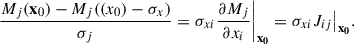
We define the Jacobian Jij to be the gradient of the residual vector rj with respect to the parameters of the solution xi (this is also the form returned by scipy.optimize.least_squares):
 (A.1)
(A.1)
where the residual vector is
 (A.2)
(A.2)
with data elements Dj (in the case considered in this paper, they are the measured spectrum at a given x − y position in the data cube, and j is the wavelength pixel index), model (fitting) function Mj (in this case a Gaussian with a background/continuum level), and the uncertainties in Dj are σj. It follows that the χ2 merit function which least squares fitting attempts to minimize (WRT the model parameter vector x) is simply
 (A.3)
(A.3)
When χ2 is equal to the number of degrees of freedom, (nf ≡ nd − np, with nd data points and np parameters in the fit), the data is fully fit by the model and further improvements to the fit are not statistically significant. The quantity χr2 = χ2/nf is called the "reduced" chi squared.
We seek to estimate the uncertainties in the model fit parameters. That is, "How much can the fit parameters change, compared to the best fit, before the change results in a statistically significant difference in the merit function?" We define statistically significant to mean that the reduced χ2 between the best fit and a new set of parameters is one. We will further make the simplifying assumption that the parameters are uncorrelated in their effect on the residuals so that we can treat their errors independently. We also assume that the errors are small so that we can linearly expand about the best fit parameters, x0. In that case the parameter change vector, σx, required to be statistically significant is easily expressed in terms of the Jacobian. χr2 = 1 gives the following starting equation:
![Mathematical equation: $$ \begin{aligned} \frac{1}{n_f}\sum _j\frac{[M_j(\mathbf x_0 )-M_j(\mathbf x_0 -\mathbf \sigma _x )]^2}{\sigma _j^2} = 1. \end{aligned} $$](/articles/aa/full_html/2026/02/aa55756-25/aa55756-25-eq6.gif) (A.4)
(A.4)
Taylor expanding about x0, for model parameter i (with uncertainty σxi), we have
 (A.5)
(A.5)
Equation (A.4) therefore yields
 (A.6)
(A.6)
With the assumption of uncorrelated error contributions from each parameter, their individual contributions to the figure of merit add in quadrature. The final estimate per parameter, with all parameters considered, is therefore
 (A.7)
(A.7)
This is the basis of the uncertainty estimate included by our line fitting code.
All Figures
|
Fig. 1. Illustration of the SPICE PSF issue in the y − λ plane. The PSF is tilted in the y − λ plane as shown in panel (b), causing leakage of signal from bright features to adjacent pixels, not strictly at the same y or λ values, as shown in panels (c) and (d). Measurements of Doppler velocity from the data in panels (c) and (d) would lead to artificial Doppler shifts, as shown in Figure 2. |
| In the text | |
|
Fig. 2. Illustration of the Doppler velocity lobes caused by SPICE PSF artifacts during a co-observing campaign between IRIS and SPICE. The SPICE data show a characteristic redshift and blueshift pattern (examples circled) around bright intensity features – compare the top left panel (IRIS) with the top right panel (SPICE), both observing the same location. This pattern similarly appears in IRIS (not shown) when the PSF from Figure 1 is applied to IRIS (not shown) and (largely) disappears when the PSF regularization method described in Plowman et al. (2023) is applied. This is strong evidence that the Doppler velocity lobes are caused by the PSF tilt out of λ and into y. |
| In the text | |
|
Fig. 3. Illustration of the x − λ and y − λ shifts in a slice of a SPICE spectral cube, with the intensity raster shown in the C III 977 Å line. Panels (b), (c), and (d) show zoomed-in slices (corresponding to the red square in panel (a)) where the x − y shift is apparent as a slight translation of the same features when scanning through consecutive wavelengths. Please see the online for an illustration of this effect. |
| In the text | |
|
Fig. 4. Schematic of the algorithm. Left panels: Representation of the original data showing the wavelength-dependent spatial shift. The line center location is shown by the green star in the middle row. Middle panels: Representation of the data after the shift (or skew) is removed, showing that a leftover spatial shift is present – the line center position has moved compared to the input. Right panels: After line fitting, the deskewing moves the position of the fit parameter images back to the original line center position. |
| In the text | |
|
Fig. 5. New correction method applied to the same dataset as in Figure 2. Top row (panels (a)): Result from a y-only wavelength shift applied with the same parameters used in the aforementioned figure. Second row (panels (b)): Results with both x and y wavelength-dependent shifts. Notably, including only the y-shift shown in panels (a) does not fully remove the Doppler velocity artifacts. In contrast, including the full x − y shift results in very good agreement between the IRIS and SPICE observations. |
| In the text | |
|
Fig. 6. De-trended Doppler shift signals, on which the figure of merit is based, for the SPICE observations used in the previous PSF work in Paper I and Figure 5. The subpanels show the resulting Doppler shifts from different shift parameters, noted above each subplot. With the highest quality Doppler shift correction around Δx = 2 arc second/Å and Δy = −2 arc second/Å this figure is consistent with the automated search determination of [2, −1.667], as shown in Figure 7. |
| In the text | |
|
Fig. 10. Example polar observations with PSF corrections for data taken on March 23, 2025. The corrections allow high-quality Doppler shift measurements to be taken at the Sun’s poles – measurements never made before – as Solar Orbiter progresses to higher latitude orbits in later phases of its mission. |
| In the text | |
|
Fig. 7. Figure of merit surface in the x − λ and y − λ shift parameter for the SPICE observations obtained during the IRIS coordinated observing campaign used for the previous PSF estimation efforts. Right panel: Figure of merit surface. Left panel: Spectral sum of the window for comparison in the C III 977 Å line. The spectral sum is calculated at each pixel by summing the intensity across all wavelengths in the spectrum. The blue points in the right panel denote where the search procedure checked the figure of merit. The figure of merit shows a clear preference for both x − λ and y − λ shifts, as confirmed by the better match to IRIS observations. |
| In the text | |
|
Fig. 8. Results of an “end-to-end” test of the new method using random test data. Top left: Doppler shifts with a nominal (no aberration) PSF. Top right: Doppler shifts with an aberrant PSF and correction, produced from the same underlying data. The correction recovers the test results well – at lower right the magnitude of the difference between the two is shown to be under 5 km/s except for very low signal regions adjacent to high signal ones. The uncorrected Doppler shifts (lower center) show far larger differences, overwhelming the actual signal in this test dataset. The line fit intensity is shown at the lower left for reference. |
| In the text | |
|
Fig. 9. Time variation of the x and y shift parameters computed in the SPICE SPROUTs observations. Upper panel: Shifts for the C III 977 Å line. Lower panel: Same, but for the relatively dim O II 718 Å line in the shortwave detector. The shifts show large changes near perihelia passages and return to a consistent background level (outside of the first ∼2 years) when the spacecraft is more distant from the Sun. The scatter in the shifts is a rough indicator of the level of uncertainty in the observations. The shifts differ between the spectral lines, indicating a wavelength or detector-position dependence in the amount of shift, although some of the difference could be due to lower S/N in the O II line. The vertical green lines show the SolO perihelia times. |
| In the text | |
Current usage metrics show cumulative count of Article Views (full-text article views including HTML views, PDF and ePub downloads, according to the available data) and Abstracts Views on Vision4Press platform.
Data correspond to usage on the plateform after 2015. The current usage metrics is available 48-96 hours after online publication and is updated daily on week days.
Initial download of the metrics may take a while.