| Issue |
A&A
Volume 706, February 2026
|
|
|---|---|---|
| Article Number | A107 | |
| Number of page(s) | 18 | |
| Section | The Sun and the Heliosphere | |
| DOI | https://doi.org/10.1051/0004-6361/202555915 | |
| Published online | 02 February 2026 | |
Peak-intensity energy spectra of intense solar energetic electron events measured with Solar Orbiter in 2020–2022
1
Department of Physics and Astronomy, University of Turku Turku, Finland
2
Leibniz-Institut für Astrophysik Potsdam (AIP) An der Sternwarte 16 D-14482 Potsdam, Germany
3
Universidad de Alcalá, Space Research Group Alcalá de Henares, Spain
★ Corresponding author: This email address is being protected from spambots. You need JavaScript enabled to view it.
Received:
12
June
2025
Accepted:
1
December
2025
Abstract
Context. The energy spectra of energetic particles offer valuable insights into particle acceleration processes. While the commonly observed spectral breaks in solar energetic electron (SEE) spectra could serve as fingerprints of the acceleration process, several transport-related effects have been proposed to be responsible as well. Here, we analyse the energy spectra of intense SEE events measured with Solar Orbiter’s Energetic Particle Detector (EPD) between December 2020 and December 2022.
Aims. We investigate the shape of SEE spectra by fitting them with various mathematical models. We compare our results with previous studies and explore possible links to transport-related effects. We aim to identify potential correlations between spectral features and meaningful parameters, such as the radial distance, or the properties of associated solar events.
Methods. We determined the background-subtracted peak-intensity spectra as observed by EPD, accounting for velocity dispersion. We fit the spectra of STEP and EPT with various mathematical models, using an automated method that chooses the best possible fit.
Results. We found four different spectral shapes in our analysis: single power law, double power law and two types of triple power law: a knee-knee (KK) and an ankle-knee (AK) triple power law. No significant correlations with radial distance were identified; although the observed spectral shapes display an ordering with the longitudinal separation between the spacecraft and the associated solar flare. We also observed a correlation between the spectral index in the intermediate energy range at 70 keV and the strength of the associated solar flare. The correlation disappears at lower and higher energies, suggesting a stronger influence of transport effects at those energies.
Conclusions. We conclude that multiple processes are likely involved in shaping SEE spectra. Our results suggest that the two breaks of the KK triple power law spectra arise from distinct effects, Langmuir-wave generation, and pitch-angle scattering, respectively. Our results also suggest that the break in the double power laws could represent a merger between the first and second breaks of KK triple power laws.
Key words: Sun: heliosphere / Sun: particle emission / solar wind
© The Authors 2026
 Open Access article, published by EDP Sciences, under the terms of the Creative Commons Attribution License (https://creativecommons.org/licenses/by/4.0), which permits unrestricted use, distribution, and reproduction in any medium, provided the original work is properly cited.
This article is published in open access under the Subscribe to Open model. This email address is being protected from spambots. You need JavaScript enabled to view it. to support open access publication.
1. Introduction
The Sun is the most efficient natural particle accelerator in our Solar System, capable of accelerating particles such as electrons and protons to relativistic energies (i.e. tens of MeV or GeV). Solar energetic particles (SEPs) are known to be accelerated at solar flare reconnection sites, as well as by shocks driven by coronal mass ejections (CMEs; Klein & Dalla 2017). One way to distinguish between these two acceleration processes of SEPs is through their energy spectra, either fluence or peak intensity. While a fluence spectrum represents the time integral of the flux over the entire event and therefore serves as a measure of the total amount of accelerated particles, the peak intensity spectrum is usually considered to more directly represent the injected spectrum at the Sun. Therefore, peak intensity spectra of Solar Energetic Electrons (SEEs) lend themselves for a direct comparison with spectra of the associated hard X-ray flare, which is assumed to be caused by the same accelerated electron population in case of pure flare acceleration (e.g. Krucker et al. 2007; Dresing et al. 2021; Wang et al. 2021). Although fluence and peak fluxes were found to be closely related (Kahler & Ling 2018) peak intensity spectra are less dominated by transport effects such as prolonged scattering, or the mixing of consecutive injections.
While the role of shocks in accelerating SEEs has been more elusive than for protons, several studies have suggested the ability of CME-driven shocks to sufficiently accelerate electrons even up to the relativistic energy range (e.g. Trotta & Burgess 2019; Dresing et al. 2022), which has also been confirmed in recent in situ observations (e.g. Jebaraj et al. 2024a,b; Raptis et al. 2025). Consequently, a clear separation of the shock-driven and flare-driven components is a major challenge in understanding SEE events. Previous studies of in situ measurements of SEE spectra have found that more often than not, the energy spectrum resembles a knee-shaped double power law (e.g. Lin et al. 1982; Krucker et al. 2009; Dresing et al. 2020; Wang et al. 2021, 2024). The break in the observed energy spectrum could be a signature of the acceleration process itself (e.g. Jebaraj et al. 2023), but it has been proposed that it is more likely caused by transport effects; specifically, the development of beam–plasma instabilities that drive electrostatic turbulence (Langmuir wave generation, Nishikawa & Riutov 1976; Kontar & Reid 2009; Krafft et al. 2013; Voshchepynets et al. 2015), or particle pitch-angle scattering, as suggested by Strauss et al. (2020).
Langmuir waves are generated by energetic electron beams propagating through the interplanetary plasma. Contrary to what has been observed, quasi-linear theory (Vedenov et al. 1962) predicts the relaxation scale of such a beam moving away from the solar corona to be only a few hundred metres. Analytical studies of beam-plasma interactions in inhomogeneous plasma (e.g. Krafft et al. 2013; Voshchepynets & Krasnoselskikh 2013; Voshchepynets et al. 2015) have shown that several physical mechanisms can influence the relaxation process. In particular, density fluctuations have been shown to play a key role in both generation and subsequent reabsorption of the generated waves (e.g. Reid & Kontar 2013; Voshchepynets et al. 2015). As a result of these processes, electrons below a certain energy threshold do not propagate freely, but are instead heavily affected by the energy loss or gain caused by wave–particle interactions. This energy loss manifests as a break in the SEE energy spectrum, primarily affecting the lower energy part.
Pitch-angle scattering, on the other hand, impacts higher-energy particles. At higher energies, particles move faster and have larger gyroradii, allowing particles to interact more efficiently with low-frequency electromagnetic waves and plasma structures in the turbulent plasma. These frequent interactions lead to a change in pitch-angle, which can cause a depletion of the electron event peak at the spacecraft, ultimately affecting the peak-intensity spectrum.
While the modelled spectral breaks were found at different energies, ∼35 keV for Langmuir wave generation (Kontar & Reid 2009) and > 100 keV for pitch-angle scattering Strauss et al. (2020), a Solar Energetic Electron (SEE) energy spectrum exhibiting signatures of two distinct transport-related breaks has not yet been reported in observations. However, different statistical studies reported differing mean spectral break energies (Krucker et al. 2009; Dresing et al. 2020), each appearing to align with one of the two proposed mechanisms. The debate continues as to which process is responsible for the observed spectral breaks, whether the cause is consistent, or varying, or a mixture of the two proposed effects (Strauss et al. 2020). It also remains unclear why a spectral break is not always present. Furthermore, modelling studies of beam-plasma instabilities in locally evolving inhomogeneous plasma have indicated that it could lead to a constantly evolving electron spectrum, bearing little resemblance to the initially injected spectrum (e.g. Krafft et al. 2013; Voshchepynets & Krasnoselskikh 2013; Voshchepynets et al. 2015; Krasnoselskikh et al. 2025).
A study focused on impulsive SEE events observed with the IMP 6, 7, and 8 spacecraft by Lin et al. (1982) found SEE spectra that resemble a knee-knee (KK) triple power law. However, the authors did not attribute the breaks in the energy spectrum to particle transport or any other energy-loss mechanism. The break energies were also high, the first one being between ∼100–200 keV and the second above 3 MeV.
Lin (1985) observed a spectrum that resembles an ankle-knee (AK) triple power law, for the SEE event on 23 September 1978 observed with ISEE-3 associated with a large solar flare. Above 10 keV, the SEE spectrum is the often-observed double power law with a knee-shaped break at ∼100 keV. However, below 10 keV the spectrum had a similar spectral index to the energies above 100 keV, forming an ankle shaped break at ∼10 keV. Lin (1985) argued that the reason for this was a secondary acceleration while the lower-energy break would reflect a break already present in the injected spectrum at the Sun. Another more recent case study by Wang et al. (2023), on a jet related SEE event observed with Wind/3DP, found a similar spectral shape with spectral breaks at Eb1 = 10.0 ± 1.7 keV and Eb2 = 56.6 ± 8.9 keV. Similarly to Lin (1985), the authors believe the spectrum to be formed already at the solar source region and do not attribute the breaks to transport effects.
Identifying all of these proposed breaks in an energy spectrum requires both a high energy resolution, but potentially also the ability to measure at different radial distances. Earlier missions, such as Wind and STEREO, likely lacked the necessary energy range and, crucially, the energy resolution to efficiently resolve the two proposed transport-related spectral breaks on a regular basis. In this study, we investigate the energy spectrum of the most intense SEE events measured by the Energetic Particle Detector (EPD; Rodríguez-Pacheco et al. 2020) on board Solar Orbiter. The instrument’s broad energy range (2 keV–30 MeV), unprecedented energy resolution, and Solar Orbiter’s varying distance from the Sun (as close as 0.28 AU) provide a unique opportunity to characterise SEE energy spectra in unprecedented detail and in regions much closer to the Sun than previously possible.
Using our newly developed fitting procedure, we investigate whether distinct spectral shapes can be identified within our sample of SEE events. We aim to determine whether the spectral shapes we find resemble those reported in previous studies and whether we are able to find a triple power law-shaped spectrum with possible signatures of both transport effects mentioned above. We also explore potential correlations between spectral features and other parameters, such as the radial distance and solar eruption characteristics.
2. Instrumentation
We used in situ electron measurements from EPD (Rodríguez-Pacheco et al. 2020) on board Solar Orbiter, which includes several sensors for electron detection: the SupraThermal Electrons and Protons (STEP) unit, the Electron Proton Telescope (EPT) and the High Energy Telescope (HET). Combining the electron intensity data from all three units enables the study of energetic electron events across an exceptionally broad energy range, from 2 keV up to 19 MeV. We determined the peak intensity to construct peak-intensity energy spectra for all energy channels of the three units, namely, STEP, EPT and HET. However, we fit data only from STEP and EPT. This decision was made due to an on-board software patch introduced to HET during the early mission phase, which led to intensity changes in the first two HET electron energy channels. These changes could lead to inconsistent spectral-fitting results. The combined energy range of STEP and EPT (2–475 keV) provides a clear advantage over previous studies (e.g. Krucker et al. 2007, 2009; Dresing et al. 2020) which used the Solar Electron and Proton Telescope (SEPT; 45–425 keV, 16 energy channels) on board STEREO, or the three-dimensional (3D) Plasma and Energetic Particle Experiment (3DP; 1–300 keV, 16 energy channels) on board the Wind spacecraft. The broader energy range and especially the significantly higher energy resolution of STEP (48 energy channels) and EPT (34 energy channels) allow us to identify potential multiple breaks within a single energy spectrum, which have not been reported before.
3. Analysis
Our analysis is divided into two primary components: (1) the construction and fitting of the energy spectra and (2) a correlation analysis and comparison of the resulting spectral features. In this section, we first outline our event selection criteria followed by a more detailed description of our spectra fitting process. Finally, we perform a correlation analysis of the spectral features found in the first part of the analysis. The details of the determination of the peak spectra are described in Appendix A. We also address the treatment of a commonly observed intensity offset in the overlapping energy range of STEP and EPT in Appendix B.
3.1. Event selection
In this study, we analysed SEE events measured by Solar Orbiter/EPD between December 2020 and December 2022. The events were selected from the CoSEE-Cat catalogue1, a list of more than 300 candidate SEE events (Warmuth et al. 2025). We selected the 50 events with the highest peak intensities at 44 keV, which lies within the overlapping energy range of STEP and EPT. Figure 1 shows the peak-intensity distribution of all events in the CoSEE-Cat catalogue until the end of 2022 measured at 44 keV with the 50 most intense events in red.
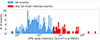 |
Fig. 1. Histogram of SEE peak intensities measured at 44 keV taken from the CoSEE-Cat catalogue. The 50 highest-intensity events that comprise the sample of our study, are shown in red. |
This selection criterion results in a high signal-to-noise ratio of the electron event above background, usually allowing for unambiguous spectral characterisation. However, counting statistics and the significance of the event in each energy channel are taken into account in the spectral analysis (see Appendix A). The 50 SEE events of our initial list are summarised in Table D.1. Six events were excluded after determining their energy spectra due to highly irregular shapes, likely resulting from the overlap of multiple electron injections, which prevented a reliable fitting.
The CoSEE-Cat catalogue includes a multitude of additional information based on Solar Orbiter measurements, for example, on the associated flares, and the presence of type II radio bursts, indicative of coronal shocks. Another parameter of interest is the distinction between gradual and impulsive events, which refers to the composition of the associated ions; in our sample, 9 out of 50 events were classified as gradual. We used several of these parameters from the catalogue in our correlation analysis. We also cross-checked the presence of type II bursts with other spacecraft using the Coordinated Radiodiagnostics Of CMEs and Solar flares (CROCS) website2.
3.2. Spectral fitting
We use the scipy.odr Boggs et al. (1989) Python package (orthogonal distance regression, ODR) to fit all energy spectra including uncertainties for both energy and intensity. The energy bin width serves as an uncertainty for the energy, and each intensity value has an uncertainty based on counting statistics. We also accounted for error propagation based on background subtraction and calculate the 95% confidence intervals for the uncertainties of the fit parameters.
Our fitting procedure includes five different mathematical models:
 (1)
(1)
 (2)
(2)
 (3)
(3)
 (4)
(4)
 (5)
(5)
Equation (1) corresponds to a single power law with power law index γ1; Equation (2) is a double power law that transitions from the power law index γ1 to the power law index γ2 after a break point at the energy Eb; Equation (3) is a single power law with power law index γ1 and an exponential cut-off with exponent x at a cut-off energy Ec; Equation (4) is a double power law transitioning between the power law index γ1 and γ2 about Eb with an exponential cut-off with exponent x at Ec; and Equation (5) is a triple power law that transitions between the power law indices γ1 and γ2 about Ebl and then again between γ2 and γ3 about the higher break energy Ebh. Here, I0 is a differential intensity defined at the reference energy E0 = 100 keV. α indicates the sharpness of the transition between γ1 and γ2, while β represents the transition between γ2 and γ3. The larger the value of α and β, the sharper the transition between spectral indices.
Equations (1)–(4) are adapted from the equations introduced by Ellison & Ramaty (1985). In Equations (3) and (4) we introduce a super exponent x as a free parameter. This allows us to fit a wider range of spectra, with weaker or stronger (sub–super) exponential cut-offs3. Figure 2 shows a visual example of the five mathematical models (Equations (1)–(5)) that we can fit to the peak-intensity spectra.
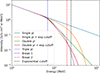 |
Fig. 2. Example of the five mathematical models included in our fitting procedure: A single power law (pl) (Equation (1)) in blue, a single power law with an exponential (exp) cut-off (x = 2, Equation (3)) in orange, a double power law (Equation (2)) in green, a double power law with an exponential cut-off (x = 2, Equation (4)) in red, and a triple power law (Equation (5)) in purple. The blue dashed line represents the break energy of the double power law and the double power law function with an exponential cut-off and the first break of the triple power law function. The dashed red line represents the break energy of the second break of the triple power law function. The dashed black line represents the exponential cut-off energies. |
For each event in this study, we determine the peak intensity spectra, as described in the previous section, three times using different time averages of 1 minute, 2 minutes, and 5 minutes. We then apply our fitting routine to each of the three differently averaged spectra independently, allowing it to determine which of the five mathematical models (Eqs. (1)–(5)) provides the best fit. The reason for including these differently averaged spectra is based on visual inspection of the time series data and trying to find an optimal balance between reducing noise and over-averaging. While comparing these differently averaged spectra, we found not only that the spectral parameters and even the resulting shape can vary but also that the apparently best time averaging varies from event to event so that we refrained from choosing one fixed averaging for all events. Instead we chose the best fit based on the reduced χr2, i.e. χ2/DOF, where DOF denotes the degrees of freedom. This value corresponds to residual variance output of the ODR function, which is equivalent to χ2/DOF. After obtaining the best-fitting model for each averaging, we compare the χr2 values and select the fit with the lowest value as the most representative of the event. The time averaging which resulted in the best fit is also listed in Table D.1.
We divided our spectra into two groups depending on the energy range we are able to fit. For some events, it is not possible to fit STEP data, either because the particle beam is not coming from the nominal sunward direction, or because most of the peak-intensity data points are not found to be significant (see above explanation). Thus, we divided our events into events that were measured and fit using both STEP and EPT data (2–475 keV) and events that were only measured and fit using EPT data (25–475 keV).
4. Results
4.1. Spectral shapes and features
Figure 3 shows examples of the four spectral shapes we identified in our sample: single power law (3 events), double power law (13 events) and two types of triple power laws: one that becomes progressively softer after each break (KK triple power law, 10 events) and one that exhibits a hardening, or plateau-like behaviour, after the first break (AK triple power law, 18 events). A complete list of events analysed, along with their corresponding spectral classifications, is provided in Table D.1. While the single and double power laws (Figs. 3a–3b) have consistently been reported by previous observations of SEE peak-intensity spectra (e.g., Lin et al. 1982; Krucker et al. 2009; Dresing et al. 2020), the two types of triple power law spectra have only seldom been reported (e.g., Lin 1985; Wang et al. 2023). Our results were enabled by EPD’s unprecedented energy resolution and broad energy coverage.
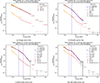 |
Fig. 3. Example spectra showcasing the four most common spectral shapes we find when fitting the peak-intensity spectra of the events in our list. (a) Single power law. (b) Double power law. (c) Triple power law (with consecutive spectral softening). (d) Triple power law with a plateau after first break. The orange, red, and maroon points represent STEP, EPT, and HET data, respectively. The fainter and lower intensity points show the pre-event background that is subtracted from the peak intensities. The grey points denote energy channels that were excluded from the fits (see Appendix A). Note: we applied the fits only in the energy range covered by STEP and EPT. The dashed vertical blue and purple lines represent the spectral breaks, and the legends provide the fit parameters. |
Table 1 summarises the statistical results of the spectral shapes and presents the mean values of the spectral features for each of the different spectral fits identified in our sample.
Average values of the spectral parameters for the different types of fits.
Surprisingly, the most common spectral shape identified in our sample is the AK triple power law (18 out of 44 events). Table 1 shows the corresponding mean parameters, subdivided into two groups: spectra analysed with a combination of STEP and EPT, along with events observed solely by EPT, resulting in a more limited energy range. Triple power law spectral shapes exhibiting a plateau in the central part have been predicted in simulations by Reid & Kontar (2013). The authors modelled the evolution of SEE spectra in the inner heliosphere, accounting for Langmuir wave generation and heliospheric plasma density fluctuations. The simulations resulted in triple power law spectral shapes for both fluence and peak-intensity spectra at distances up to ∼50 solar radii (closer to the Sun than any of the events in our sample), which evolved into a double power law at larger distances. Reid & Kontar (2013) reported that the spectral plateaus are a consequence of inhomogeneous background plasma, which can cause part of the electron beam to gain energy via the absorption of Langmuir waves. The energy range of the plateaus found by Reid & Kontar (2013) lies between 30 keV and 40 keV, aligning roughly with the energy ranges found in our study, on average between ∼30 keV and ∼70 keV. Reid & Kontar (2013) noted, however, that both the energy range of the plateau and the distance over which it can still be observed, strongly depend on the input parameters of the model. The authors found that with a radially decreasing density, the peak spectrum forms a clear plateau between 10–40 keV at 1.2 AU in the extreme case of no density fluctuations. When a large number of density fluctuations are included, however, the spectrum resembles instead a double power law. We further investigated potential dependencies on radial distance to the Sun and longitudinal separation with respect to the source region in Sect. 4.2.
Figure 4 shows histograms of the break energies, spectral indices, and the difference of the spectral indices of the double (top row) and triple power law fits (centre row: KK triple power laws, bottom row: AK triple power laws). Interestingly, in examining the first column of the figure, a comparison between the break energies of the double power law (top) and the KK triple power law fits (centre), reveals that most break energies of the double power laws are located between the first and second break of the KK triple power law fits. The mean break energy of the double power law fits (see Table 1) is Eb = 67.8 ± 1.7 keV, while the break energies of the KK triple power law fits are Ebl = 28.8 ± 0.5 keV and Ebh = 100.6 ± 1.6 keV, respectively. This could suggest that the double power law events in our sample represent, in principle, the same type of events as the KK triple power law events, but with spectral breaks that are too close to be resolved individually, resulting in a single apparent spectral transition. Although we divided events based on whether they were measured solely with EPT or with a combination of STEP and EPT, we did not see any significant difference in the resulting values of the spectral parameters of the double power law fits (see Table 1). However, a clear difference emerges when making the same distinction for the AK triple power laws (see Table 1), particularly with respect to the spectral break energies. As expected, the combination of STEP and EPT allows the identification of lower energy spectral breaks that fall outside EPT’s measurement range, likely explaining the higher break energies observed in EPT-only events. It is worth noting, however, that only three events in our sample were identified as AK triple power laws using only EPT alone (Column 8, Table 1).
The spectral indices of the double power law and KK triple power law events show some similarities (see Table 1 and Fig. 4). The average value of γ1 for all double power law events combined (γ1 = −2.13 ± 0.10) is the same, within error bars, as γ1 for the KK triple power law events. In addition, γ2 of the double power law fits (γ2 = −4.60 ± 0.06) is close to γ3 of the KK triple power laws (γ3 = −4.29 ± 0.05). This further supports the interpretation that the double power law events represent the same type of events as the KK triple power laws, but the two spectral breaks have merged into one.
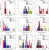 |
Fig. 4. Distributions of (Column 1) break energies, (Column 2) spectral indices (γ1, γ2, and γ3), and (Column 3) the absolute value of the difference between the spectral indices, which represents the magnitude of the spectral change between spectral indices, of the double power law fits (row 1), of the triple power law fits that become progressively softer (row 2), and the triple power law fits that have a plateau or spectral hardening after the first break (row 3). The events measured only by EPT are marked by black hatching. |
The softest spectra found in our sample correspond to the AK triple power laws, with an average value for the indices of γ1 = −6.23 ± 0.73 and γ3 = −4.81 ± 0.32. The average value for γ2 is −0.15 ± 1.02. The value is very close to zero, which is why we refer to it as a plateau. However, as shown by the large uncertainty of the average γ2 value, not all events exhibit a plateau but some only show a spectral hardening after the first break.
The spectral indices of the double power law fits, γ1 = −2.13 ± 0.44 and γ2 = −4.60 ± 0.06 as well as γ2 = −3.00 ± 0.03 and γ3 = −4.29 ± 0.05 of the KK triple power law fits are in good agreement with the values reported by Dresing et al. (2020), who found average spectral indices of γlow = −2.53 and γhigh = −3.93 based on electron measurements of STEREO/SEPT4. However, the average break energy of the double power law fits, as well as both break energies of the KK triple power law fits, are lower than the value reported by Dresing et al. (2020), who found a break energy of approximately Eb ≈ 120 keV. For comparison, the average value of the second break of the KK triple power law fits that we find is Ebh = 100.6 ± 1.6 keV.
We note that the average values calculated in Table 1 are the arithmetic mean values of each parameter and the corresponding uncertainties are calculated using the error propagation of a mean (with noise5). The motivation for using the arithmetic means is to enable a direct comparison with previous studies. Another way to calculate the average values is to use the inverse-variance weighted average, which takes into account the uncertainties of the fit results. For details, see Appendix E, where we provide the mean values using inverse-variance weighted averaging.
4.2. Correlation analysis
In this section, we investigate potential correlations between the various spectral features and parameters of the associated solar events with the aim of gaining insight into the mechanisms behind the different spectral breaks and the various spectral shapes found in our sample. In Figs. 5–C.2 we distinguish between spectra that progressively soften after each break (on the left) and spectra that exhibit a plateau or hardening after the first break (on the right).
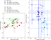 |
Fig. 5. Dependence between the spectral indices before and after the spectral breaks. Left: Double power law fits (red). KK triple power law fits (green, with the first and second break in different shades). Right: Spectral index values for triple power laws with a plateau-like structure. The different shades represent the spectral indices on both sides of the first and second break. Spectra that were determined with EPT only are marked with black circles. |
Figure 5 presents the spectral indices above the break energy plotted against the spectral indices below the break. Several studies (Krucker et al. 2009; Kontar & Reid 2009; Dresing et al. 2020) have found a positive correlation between the two spectral indices. This is not evident in all events in our study (Fig. 5, left panel), especially when considering the different spectral shapes separately. We see a slight positive trend for the first break of the KK triple power law events (dark green points), whereas no clear trend is apparent for the double power law events (red points). In contrast, we see a clear separation between the two spectral transitions for the AK triple power law fits (dark and light blue points), with a rather negative correlation. This highlights how much the spectral index changes before and after the plateau. Furthermore, the range of spectral values of the AK triple power law fits is also three times broader than that of the left-hand plot (comparing the x-axes of Figure 5), including positive and strongly negative spectral values.
Figure 6 shows the intensity at the break energy versus the break energy. As discussed in the previous section, it is evident from this plot as well that most break energies of the double power law fits (in red) lie between the two breaks of the KK triple power law fits. Kontar & Reid (2009) have suggested that, if a spectral break is caused by Langmuir-wave generation, we should see an anti-correlation between the intensity at the break energy and the break energy itself. This is because a high beam density (higher electron intensities) would result in a more rapid generation of electrostatic waves in the plasma and a stronger interaction between these and the electrons (Kontar & Reid 2009), thus producing a break at lower energies. It should be noted that in this context Kontar & Reid (2009) only refer to spectra that become softer after the break. The left panel of Figure 6 shows such an anti-correlation for the first break (dark green points) of the KK triple power law and to some extent for the double power law spectra (red points). We also calculated the Spearman correlation coefficient using a Monte Carlo method that takes into account the fit uncertainties of the break energies. We found a correlation coefficient of −0.47 ± 0.16 for the double power law breaks and a correlation of −0.81 ± 0.12 for the first break of the KK triple power law fits. We do not find a significant correlation for the high-energy break of the KK triple power law (light green points) or the breaks of the AK triple power laws (blue points, on the right). This plot is clear example of the distinct behaviour and characteristics of the AK triple power law, shown on the right side, in comparison to the KK triple power law.
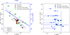 |
Fig. 6. Break energies as a function of the intensity at the break energy. Symbols and colours are the same as in Figure 5. The spearman correlation coefficient for the double power law (red points) is –0.47 ± 0.16 and the one for the first break of the KK triple power law (dark green points) is –0.81 ± 0.12. For comparison, we also overplot the fits of the single-law events (pl 1, 2 and 3) found in this study. Single pl 1 (continuous blue line): 2021-10-28, single pl 2 (dotted blue line): 2022-07-23, single pl 3 (dashed blue line): 2022-08-30. |
The left panel of Figure 6 also includes a real representation of the single power law spectra found in our analysis, which we overplot based on their occurrence in the same intensity-energy space like the break points. The energy ranges of the single power laws plotted here, are representative of the real energy range fit for each event. As mentioned in Appendix A, it was sometimes necessary to exclude some energy channels from the fit due to different reasons. Although HET energies are not considered in the spectral fits of our analysis, they are still included in the spectra we used for the visual inspection, as shown in Figure 3. In the case of the three single power law events, all three extend to energies in the HET range. The continuous blue line (Fig. 6, left), representing the spectral fit for the event on 28 October 2021 (shown also in Fig. 3a), covering the full energy range of STEP and EPT (the broadest out of the three single power law fits) and extends to the full HET energy range as well. However, at HET energies there is a clear depletion, suggesting that the higher energy break is pushed to high energies. The event on 23 July 2022 (dotted blue line) is a very similar case. It covers almost the full STEP and EPT range and extends to HET energies as well. There is a slight depletion at HET energies, less pronounced than in the previous case. The dashed blue line represents the event on 30 August 2022 measured with EPT south. Having to exclude STEP does not allow us to find any possible breaks at lower energies, but similarly to the previous cases, there is an evident depletion in the HET range.
Strauss et al. (2020) studied the effects of pitch-angle scattering on SEE spectra, finding that the influence of this process increases with distance from the Sun. This is because a greater travel distance for SEEs allows for more scattering to occur. A spectral break caused by pitch-angle scattering is therefore expected only to be observed at larger distances from the Sun and it is predicted to become more pronounced with increasing distance. This could result in a lower break energy and a larger difference in spectral index across the break. We therefore examined possible correlations with Solar Orbiter’s radial distance from the Sun. However, we did not find any significant dependence of these parameters on distance (see Appendix C).
In Fig. 7, we investigate whether the spectral shape depends on the distance from the Sun or the longitudinal separation to the associated flaring region. The figure shows Solar Orbiter’s radial distance as a function of the absolute longitudinal separation angle between the spacecraft’s magnetic footpoint at the Sun and the location of the associated flare, as provided by the CoSEE-Cat catalogue. We mark events associated with type II radio bursts with a diamond shape. Overall, there is no clear distinction between the different spectral shapes with respect to radial distance. However, in terms of longitudinal separation, it is noteworthy that the single–power-law spectra (yellow points), although limited to only three events, correspond to the largest separation angles in our sample and are observed exclusively at angles > 66°. These single power law events are also all associated with a type II radio burst and are all classed as gradual events in the CoSEE-Cat catalogue, suggesting a potential shock-related source. Furthermore, double power law events are only observed up to separation angles of about 40°, while the KK triple power laws (green points) are only observed at very small longitudinal separations (< 12°), but across all distances.
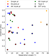 |
Fig. 7. Longitudinal separation angle (absolute value) between the spacecraft’s magnetic footpoint at the Sun and the flare location versus the spacecraft’s distance. The different colours represent different spectral shapes of the events. Spectra determined with EPT only are contoured in black. The events with a type II radio burst are diamond shaped. Not all events are included in the plot, as we are unable to calculate the separation angle for some events due to missing information on the flare location. |
Following the work of Dresing et al. (2020), Rodríguez-García et al. (2023), we determined the spectral index at a reference energy of 70 keV and 200 keV, respectively. We also determined the spectral indices at a much lower reference energy of 10 keV. This approach enables a comparison of the spectral indices of the different events regardless of their spectral shapes. In Fig. 8 we plot these spectral indices as a function of the soft X-ray peak flux of the associated flares. Events associated with type II radio bursts are indicated with black circles. At the reference energy of 70 keV, we can see a clear trend of harder spectra being associated with stronger flares, suggesting a more efficient electron acceleration. This trend is less apparent at 10 keV and 200 keV. Moreover, the most intense flares are accompanied by type II radio bursts, indicating the presence of a shock. We would expect that SEE events with harder spectral indices involve shock acceleration (e.g. Oka et al. 2018), while flare acceleration would be responsible for the softer spectra. Although the softest spectral indices in Fig. 8 are not associated with type II bursts (and many of the hardest spectral indices are accompanied by a shock), we did not find a clear distinction between events with and without the presence of type II bursts.
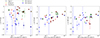 |
Fig. 8. Spectral index as a function of the soft X-ray peak flux of the associated flare. Left: Spectral index at a fixed energy of 10 keV. Middle: Spectral index at 70 keV. Right: Spectral index at 200 keV. The different colours represent different spectral shapes. Events accompanied by a type II burst are marked in black. Not all events are included in this plot, as we do not have a measurement for the soft X-ray peak flux for all events. In case the spectral index of the AK triple power law (blue), at any of the fixed energies, falls within the plateau region, we exclude it from this plot. |
In addition to hard spectral indices, the maximum energy can be considered indicative of the efficiency of the acceleration process. We identified the maximum energy of each event during the determination of the peak-intensity spectra (see Appendix A) as the highest energy channel (excluding HET) with a significant intensity peak above pre-event background. Figure 9 shows that indeed, the events with the highest maximum energies are accompanied by type II bursts (diamonds). However, similar to Fig. 8, the association is not particularly distinct. Several high-energy events lack a type II burst, while several lower energy events are accompanied by one.
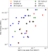 |
Fig. 9. Maximum energy at which each event is seen as a function of the soft X-ray peak flux of the associated flare. The different colours represent the different spectral shapes. Spectra analysed with EPT only are marked in black. The events with a type II radio burst are diamond shaped. Not all events are included in this plot, as we do not have a measurement for the soft X-ray peak flux for all events. |
5. Discussion and conclusions
SEE spectra, their shape in particular, can potentially provide significant insights into the acceleration and transport of electrons. Our study considers a sample of 50 intense SEE events observed by Solar Orbiter. We determined the peak-intensity spectra for each event and fit each one with various models. The best-fitting model was then automatically selected by comparing the reduced χr2. Spectral parameters such as break energies, spectral indices, and the overall spectral shape were then analysed with respect to the spacecraft’s distance to the parent source, as well as source characteristics, in order to shed light on the processes behind different spectral features. The energy resolution of Solar Orbiter/EPD measurements, combined with the spacecraft’s varying distance from the Sun, allowed us to study SEE spectra with unprecedented detail.
Interestingly, among the 44 spectra that could be successfully fit, the majority (28 events) exhibited triple power law spectra featuring two spectral breaks. The second most common spectral shape was a double power law (13 events). Additionally, three spectra were consistent with a single power law shape. Based on their distinct characteristics, we further divided the triple power law spectra into two categories: (1) a triple power law that becomes progressively softer after each spectral break (KK triple power law, 10 events, Fig. 3c); and (2) a triple power law that presents a spectral hardening, almost plateau-like structure, after the first spectral break (AK triple power law, 18 events, Fig. 3d).
The average break energy, Eb = 74.3 ± 1.6 keV, of the double power law spectra is consistent with the results of Krucker et al. (2009), who studied SEE spectra using observations of Wind/3DP and found an average break energy of ∼60 keV. Kontar & Reid (2009) simulated the effects of Langmuir waves on SEE spectra to reproduce the results of Krucker et al. (2009), resulting in spectra with breaks between 4–80 keV and spectral indices remarkably similar to the observations of Krucker et al. (2009).
Although the average value of the lower energy break in the KK triple power law spectra (Ebl = 30.9 ± 1.7 keV) is considerably lower than the value we report for the double power law spectra, Ebl is still within the range of possible spectral break energies found by Kontar & Reid (2009). A further argument supporting the generation of Langmuir waves causing the lower energy break in the KK triple power laws is the close agreement between the spectral index and simulation results. We found a spectral index below the break of γ1 = −2.13 ± 0.10, which aligns well with the modelled expectation of ∼ − 2.
Furthermore, we found a strong anti-correlation between the energy of the first spectral break and the electron intensity at the break energy of the KK triple power laws (Spearman correlation coefficient: –0.81 ± 0.12; see Fig. 6). The same anti-correlation is not as evident in the case of double power law spectra. According to Kontar & Reid (2009), such an anti-correlation is a clear indication that the spectral break is caused by Langmuir waves.
Dresing et al. (2020) did not find such anti-correlation in their statistical study of SEE events using STEREO/SEPT data. They also found a significantly higher mean energy for their double power law spectral breaks of ∼120 keV. This led Strauss et al. (2020) to suggest that these breaks could be caused by pitch-angle scattering instead. The average value of the second break of our KK triple power law spectra is Ebh = 97.6 ± 17.7 keV, which is close to the value found by Dresing et al. (2020). Moreover, the spectral indices γlow = −2.53 and γhigh = −3.93 found by Dresing et al. (2020) resemble the average values we found, namely, γ2 = −2.7 ± 0.2 and γ3 = −4.1 ± 0.5 of the KK triple power law spectra quite closely. These findings suggest that the KK triple power law spectra identified in our analysis could result from a combination of the two different transport effects discussed above. This scenario was previously proposed by Strauss et al. (2020) and Dresing et al. (2021), who speculated that this observation would become possible with better instrumentation. When comparing the average break energies of the KK triple power law and the double power laws, we find that the break energy of the latter falls between the two break energies of the KK triple power law. This suggests that the break of the double power law spectra could be a composite feature, representing a merger of the two breaks observed in the KK triple power law events.
Theory suggests that in the case of Langmuir-wave generation, the spectrum is altered primarily at energies below the break; whereas in the case of pitch-angle scattering, the spectrum would change mainly at energies above the break. This implies that the part of the KK triple power law spectra between the two breaks would most closely reflect the injected spectra at the Sun. This interpretation is supported by Fig. 8 where we compared the spectral indices with the soft X-ray peak flux of the associated flares and the presence of coronal shocks marked by the observation of type II radio bursts to study the potential imprint of the acceleration process on the observed spectra. Following the work of Dresing et al. (2020), Rodríguez-García et al. (2023), we studied such correlations using the spectral indices measured at three reference energies, 10 keV (γ10), 70 keV (γ70), and 200 keV (γ200), combining all events in our sample regardless of their spectral shape. At the reference energy of 70 keV, which represents the energy regime between the two breaks of the KK triple power laws, we can see the clearest correlation of spectral indices with the flare strength. This correlation is less evident at lower and higher energies suggesting a stronger influence of transport effects leading to an alteration of the observed spectra.
The AK triple power law spectra, which make up the largest portion of our events (16 events), seem to exhibit completely different characteristics. One of the most evident differences is the lack of any correlation between the break energy and the intensity at the break (see Fig. 6). Furthermore, the AK triple power laws have much softer spectral indices (γ1 and γ3) and are rarely associated with a type II radio burst (two events, see Figs. 7–9).
There have been very few mentions of triple power law spectra in previous SEE studies. Using observations by IMP 6, 7, and 8 Lin et al. (1982) reported KK triple power law spectral shapes in a few strong flare events, with break energies located at significantly higher energies with Eb1 ≥ 100 keV and Eb2 ≥ 1 MeV. The lower-energy break is in a similar range to other reported values, however the spectral indices below and above the break are much harder. The values range between –0.6 and –1.1 below the break and –2.4 and –2.8 above the break. Furthermore, their spectra are event-integrated spectra, in contrast to our peak intensity spectra. In a later study on SEE spectra observed with ISEE-3, again associated with strong flares, Lin (1985) found instead a spectral shape resembling an AK triple power law. The break energies were at Eb1 ∼ 10 keV and Eb2 ∼ 100 keV. The authors pointed out that the spectrum above 10 keV, resembled the typically observed double power law. However, the author suggested that the lower-energy part of the spectrum, including the ankle-shaped break at 10 keV, reflects the injected spectrum at the Sun.
In a case study of an SEE event observed with Wind/3DP and associated with solar jets, Wang et al. (2023) found an AK triple power law spectrum with a lower break at Eb1 = 10.0 ± 1.7 keV, similar to the one found by Lin (1985). However, the authors found the higher-energy break to be at Eb2 = 56.6 ± 8.9 keV, compared to the ∼100 keV reported by Lin (1985). However, the value is similar to Ebh = 60.1 ± 4.4 keV found in our study. Wang et al. (2023) do not attribute the breaks in the spectrum to transport effects but argue that the spectrum is rather the direct representation of the injected spectrum at the Sun.
Similar spectral shapes have been found in simulations of SEE events. Reid & Kontar (2013) found this specific type of spectra to result from Langmuir wave generation in the inner heliosphere at radial distances from the Sun of less than ∼20 R⊙, demonstrably closer than in our measurements. Building on the gas–dynamical framework of Ryutov & Sagdeev (1970), it was shown by Reid & Kontar (2013) that such spectra would develop into a double power law farther out in the heliosphere. However, given the importance of randomly inhomogeneous plasma in shaping the electron energy spectra, any variation in the level of density fluctuations leads to a change in the evolution of the beam and, consequently, its spectral shape (Voshchepynets et al. 2015; Krasnoselskikh et al. 2025).
To illustrate this, Reid & Kontar (2013) implemented a radially decreasing background density and compared electron spectra (peak and fluence) at 1.2 AU, with and without fluctuations. In the unphysical homogeneous limit of no fluctuations, the simulation produces excessive Langmuir wave growth and a pronounced spectral plateau between 10 keV and 40 keV. Clearly, a scenario without any density fluctuations is unrealistic in the solar wind (Sishtla et al. 2023), but in case of relatively low density fluctuations, the authors show that such beam-plasma structures could be observed as far as 4.3 AU. The AK triple power-law events that we report here are consistent with these modelling results of flare accelerated electrons with which type II bursts are rarely observed (Reid & Kontar 2013).
If the AK triple power laws would directly resemble the injected spectra at the solar source, as suggested by Lin (1985), Wang et al. (2023), we would also expect to see a correlation between the spectral index at low energies (10 keV) and the soft X-ray peak. As illustrated in Figure 8, this is not the case. The spectral indices at 70 keV, which on average corresponds to the part of the AK triple power law spectrum above both break, correlates more clearly with the soft X-ray peak flux, further reinforcing the theory that the lower part of the spectrum is affected by Langmuir wave generation.
Another possible explanation for such a spectral shape (AK triple power law) could be the mixing of two or more separate SEE events occurring so close in time to each other that they can no longer be separated in the time-series observations. We specifically checked for the potential overlap of two electron beams and excluded energy channels and potentially dubious events.
The single power law spectra we found in our study appear to be even more puzzling, as they seem to result from a lack of transport effects or a shift of transport-related breaks outside of the studied energy range. The spectra of these three events are shown in Figure 6. The spectra of all three events (28 October 2021, 23 July 2022, and 30 August 2022) exhibit a depletion at HET energies, suggesting the shift of a possible pitch-angle-related spectral break to higher energies. The energy range of the 30 August 2022 event is limited to the EPT range; thus, it is not possible to draw any conclusions on the presence or absence of a low-energy break. However, such low-energy break is absent for the other two events.
Intriguingly, although limited to just three cases, all single power law spectra correspond to observations taken at large longitudinal separation angles with respect to the associated flare longitude (see Fig. 7). They are also all associated with a type II burst and are classified as gradual events in the CoSEE-Cat catalogue. In contrast, the KK triple power laws are only found at the smallest separation angles (< 12°). This suggests that, in order to observe the two breaks in the spectra the spacecraft needs to be well connected to the associated flaring source region. Conversely, at larger longitudinal separations, the electron beam could become too dilute to generate Langmuir waves, resulting in the absence of this spectral break.
Our study clearly shows the enhanced capabilities of new generation energetic particle instrumentation such as that provided by Solar Orbiter/EPD. The increased energy range of SEE measurements and particularly the unprecedentedly high energy resolution enabled us to characterise SEE spectra in great detail, revealing new spectral shapes such as the KK triple power laws in the studied energy range, and the variability of spectral shapes. Although the energy range of STEREO/SEPT is very similar to the one of EPT, Dresing et al. (2020) did not find a triple power law spectrum. However, we identified such a spectral shape even in one event analysed using only EPT, highlighting the beneficial impact of having access to a fine energy resolution.
We note that our sample of 50 events only includes the most intense events listed in the CoSEE-Cat catalogue until the end of 2022. As shown in Figure 1, the events selected for this study are a few orders of magnitude higher in intensity than the average event in the catalogue. Our selection criterion was chosen with the aim of determining clear SEE spectra based on high counting statistics; however, this could introduce a bias to our study and results. A more comprehensive statistical analysis of all events in the CoSEE-Cat catalogue will be the focus of future work, aimed at improving our understanding of SEE events. Furthermore, our study opens the door for more in-depth comparison of in situ SEE spectra with solar eruption characteristics, most importantly the spectral characteristics of associated hard X-ray flares as done in previous studies using older-generation electron instruments (e.g., Krucker et al. 2007; Dresing et al. 2021). Very valuable for these future analyses are our results on which energy range should be used for such comparisons. As shown in Fig. 8 an intermediate energy range of around 70 keV shows the clearest correlation with the associated solar flare strength, while the correlation vanishes at lower and higher energies, presumably due to transport effects. Detailed comparisons of SEE spectra with solar flare HXR spectra as well as with other eruption parameters will permit new insights into the relation of the SEEs with their solar sources and help to uncover the relative roles of flares and shocks in SEE events, which is a long-standing issue in SEP physics.
Acknowledgments
We acknowledge funding from the European Union’s Horizon Europe research and innovation programme under grant agreement No. 101134999 (SOLER). The paper reflects only the authors’ view and the European Commission is not responsible for any use that may be made of the information it contains. We acknowledge funding from the Vilho, Yrjö and Kalle Väisälä Foundation of the Finnish Academy of Science and Letters. We acknowledge the funding from the Finnish Cultural Foundation. Work in the University of Turku was performed under the umbrella of Finnish Centre of Excellence in Research of Sustainable Space (FORESAIL) funded by the Research Council of Finland (grant No. 352847). We further acknowledge support by the Research Council of Finland (SHOCKSEE, grant No. 346902 and AIPAD, grant No. 368509). We also thank the members of the data analysis working group at the Space Research Laboratory of the University of Turku, Finland for useful discussions. I.C.J. is grateful for support by the Research Council of Finland (X-Scale, grant No. 371569) and support from ISSI’s “Visiting Scientist Program”. R.G.H. and F.E. acknowledge the financial support by project PID2023-150952OB-I00 funded by MICIU/AEI/10.13039/501100011033 and by FEDER, UE.
References
- Bevington, P. R., & Robinson, D. K. 2003, Data Reduction and Error Analysis for the Physical Sciences (McGraw-Hill) [Google Scholar]
- Boggs, P. T., Byrd, R. H., Donaldson, J. R., & Schnabel, R. B. 1989, User’s reference guide for ODRPACK::software for weighted orthogonal distance regression version 1.7 (National Institute of Standards and Technology) [Google Scholar]
- Dresing, N., Effenberger, F., Gómez-Herrero, R., et al. 2020, ApJ, 889, 143 [NASA ADS] [CrossRef] [Google Scholar]
- Dresing, N., Warmuth, A., Effenberger, F., et al. 2021, A&A, 654, A92 [NASA ADS] [CrossRef] [EDP Sciences] [Google Scholar]
- Dresing, N., Kouloumvakos, A., Vainio, R., & Rouillard, A. 2022, ApJ, 925, L21 [NASA ADS] [CrossRef] [Google Scholar]
- Ellison, D. C., & Ramaty, R. 1985, ApJ, 298, 400 [Google Scholar]
- Jebaraj, I. C., Dresing, N., Krasnoselskikh, V., et al. 2023, A&A, 680, L7 [NASA ADS] [CrossRef] [EDP Sciences] [Google Scholar]
- Jebaraj, I. C., Agapitov, O., Krasnoselskikh, V., et al. 2024a, ApJ, 968, L8 [NASA ADS] [CrossRef] [Google Scholar]
- Jebaraj, I. C., Agapitov, O. V., Gedalin, M., et al. 2024b, ApJ, 976, L7 [NASA ADS] [CrossRef] [Google Scholar]
- Kahler, S. W., & Ling, A. G. 2018, Sol. Phys., 293, 30 [NASA ADS] [CrossRef] [Google Scholar]
- Klein, K.-L., & Dalla, S. 2017, Space Sci. Rev., 212, 1107 [Google Scholar]
- Kontar, E. P., & Reid, H. A. S. 2009, ApJ, 695, L140 [NASA ADS] [CrossRef] [Google Scholar]
- Krafft, C., Volokitin, A. S., & Krasnoselskikh, V. V. 2013, ApJ, 778, 111 [NASA ADS] [CrossRef] [Google Scholar]
- Krasnoselskikh, V., Jebaraj, I. C., Cooper, T. R. F., et al. 2025, ApJ, 990, 100 [Google Scholar]
- Krucker, S., Kontar, E. P., Christe, S., & Lin, R. P. 2007, ApJ, 663, L109 [CrossRef] [Google Scholar]
- Krucker, S., Oakley, P. H., & Lin, R. P. 2009, ApJ, 691, 806 [NASA ADS] [CrossRef] [Google Scholar]
- Krucker, S., Hurford, G. J., Grimm, O., et al. 2020, A&A, 642, A15 [NASA ADS] [CrossRef] [EDP Sciences] [Google Scholar]
- Lin, R. P. 1985, Sol. Phys., 100, 537 [NASA ADS] [CrossRef] [Google Scholar]
- Lin, R. P., Mewaldt, R. A., & Van Hollebeke, M. A. I. 1982, ApJ, 253, 949 [NASA ADS] [CrossRef] [Google Scholar]
- Nishikawa, K., & Riutov, D. D. 1976, J. Phys. Soc. Jpn., 41, 1757 [Google Scholar]
- Oka, M., Birn, J., Battaglia, M., et al. 2018, Space Sci. Rev., 214, 82 [NASA ADS] [CrossRef] [Google Scholar]
- Parker, E. N. 1958, ApJ, 128, 664 [Google Scholar]
- Raptis, S., Lalti, A., Lindberg, M., et al. 2025, Nat. Commun., 16, 488 [Google Scholar]
- Reid, H. A. S., & Kontar, E. P. 2013, Sol. Phys., 285, 217 [NASA ADS] [CrossRef] [Google Scholar]
- Rodríguez-García, L., Gómez-Herrero, R., Dresing, N., et al. 2023, A&A, 670, A51 [NASA ADS] [CrossRef] [EDP Sciences] [Google Scholar]
- Rodríguez-Pacheco, J., Wimmer-Schweingruber, R. F., Mason, G. M., et al. 2020, A&A, 642, A7 [Google Scholar]
- Ryutov, D., & Sagdeev, R. 1970, Sov. Phys. JETP, 31, 396 [Google Scholar]
- Sishtla, C. P., Jebaraj, I. C., Pomoell, J., et al. 2023, ApJ, 959, L33 [Google Scholar]
- Strauss, R. D., Dresing, N., Kollhoff, A., & Brüdern, M. 2020, ApJ, 897, 24 [NASA ADS] [CrossRef] [Google Scholar]
- Trotta, D., & Burgess, D. 2019, MNRAS, 482, 1154 [NASA ADS] [CrossRef] [Google Scholar]
- Vedenov, A. A., Velikhov, E. P., & Sagdeev, R. Z. 1962, Nucl. Fusion, Suppl., 4726983 [Google Scholar]
- Voshchepynets, A., & Krasnoselskikh, V. 2013, Ann. Geophys., 31, 1379 [Google Scholar]
- Voshchepynets, A., Krasnoselskikh, V., Artemyev, A., & Volokitin, A. 2015, ApJ, 807, 38 [NASA ADS] [CrossRef] [Google Scholar]
- Wang, W., Wang, L., Krucker, S., et al. 2021, ApJ, 913, 89 [NASA ADS] [CrossRef] [Google Scholar]
- Wang, W., Battaglia, A. F., Krucker, S., & Wang, L. 2023, ApJ, 950, 118 [NASA ADS] [CrossRef] [Google Scholar]
- Wang, W., Wang, L., Li, W., et al. 2024, ApJ, 969, 164 [Google Scholar]
- Warmuth, A., Schuller, F., Gómez-Herrero, R., et al. 2025, A&A, 701, A20 [NASA ADS] [CrossRef] [EDP Sciences] [Google Scholar]
When x = 1, the cut-off is exponential. For x < 1, the cut-off is sub-exponential, conversely, for x > 1 the cut-off is super-exponential.
Dresing et al. (2020) noted that using the STEREO/SEPT instrument restricted the energy range, where spectral breaks could be determined to values > 70 keV.
This means that each measurement comes with its own uncertainty. In our analysis, each spectral fit provides a parameter value (e.g., the break energy) along with its uncertainty. When determining the average value of a parameter for the full set of events, we take into account these individual uncertainties to obtain the mean and its uncertainty. For an arithmetic mean  of N values xi, with uncertainties σi, the uncertainty is
  (see Bevington & Robinson 2003).
Eq. A.1 was derived based on the Parker spiral formula (Parker 1958) using the geometric concept of an Archimedian spiral.
We note that energy-dependent background intervals such as shown in Fig. A.1 are not necessary in quiet times. However, in case of variable and decaying background intervals the choice of energy-dependent intervals, which follow also the expected trend of velocity dispersion, allow us to chose the immediate background directly before the respective intensity increase in each energy channel, which would not be possible if a fixed window would be used for all energy channels. The background is typically comparable to, or slightly longer than, the search window (approximately 1 hour). The appropriate length is decided upon manual inspection.
Appendix A: Determination of the peak spectra
To construct the peak-intensity spectrum for an event, we first determine the electron peak intensity for each energy channel of STEP, EPT, and HET. Figure A.1 shows the intensity-time series of a few selected energy channels of STEP for an example event and the pitch-angle coverage of the instrument in the lower panel. For each energy channels, we determine a value for the peak intensity, which contributes a single data point to the overall energy spectrum. This is done by automatically detecting the maximum intensity within a defined time interval, referred to as the search window, specific to each channel. The timing of these windows accounts for velocity dispersion, as electrons of different energies travel at different speeds and therefore arrive at different times.
To define the time intervals of the expected SEE peaks, we assume that the electron injection at the Sun occurs simultaneously with the event-associated flare, observed by the Spectrometer/Telescope for imaging X-rays (STIX; Krucker et al. 2020) and listed in the CoSEE-Cat catalogue. Here, we assume that all particles were injected at the same time. Based on the injection time, we estimate the electrons’ travel times by accounting for their speed-dependent propagation along nominal Parker spiral. We calculate an approximate value for the Parker spiral length6L, which serves as a lower limit for the electron travel distance, expressed as:
![Mathematical equation: $$ \begin{aligned} \begin{split} L = \frac{1}{2} \frac{v_{\rm sw}}{\Omega } \cdot \Bigg [ \frac{\Omega }{v_{\rm sw}} r \sqrt{r^2 \left( \frac{v_{\rm sw}}{\Omega } \right)^2+1} \\ + \ln \left( \frac{\Omega }{v_{\rm sw}} r +\sqrt{\left( \frac{\Omega }{v_{\rm sw}} \right)^2 r^2 +1} \right) \Bigg ] \end{split} \end{aligned} $$](/articles/aa/full_html/2026/02/aa55915-25/aa55915-25-eq8.gif) (A.1)
(A.1)
where Ω is the solar rotation frequency, vsw is the solar wind speed (assumed to be 400 km/s), and r is the distance from the Sun’s surface.
Next, we calculated the relativistic speed of electrons using the correction coefficient, βi, for electrons with energy, Ek, i, where i is the index of the energy channel:
 (A.2)
(A.2)
 (A.3)
(A.3)
Here Ek, i is the kinetic energy of the electrons in the energy channel i, me, 0 is the rest mass of an electron, c is the speed of light, and vi is the speed of an electron with kinetic energy, Ek, i. Knowing the travel distance, L, the particle velocities, vi, and the injection time, Tinj, at the Sun, we can estimate the electron travel time, Ti, to the spacecraft for each energy channel i:
 (A.4)
(A.4)
These calculations were performed for each energy channel of STEP, EPT and HET using the channel’s geometric mean energy to define the optimal search window (vertical black lines in Figure A.1) for each energy bin. The length of the search window is often case-dependent and decided upon manual inspection of the intensity timeseries as shown in the example of Figure A.1. Typically, we use a 40-minute search window starting about 20 minutes before the expected peak and ending 20 minutes after. We tried to avoid having the search window start too close to the peak time. However, the length of the search window depends primarily on two factors: (1) the presence of nearby intensity peaks from separate events, in which case the window can be shortened to about 15 minutes or less to avoid catching multiple peaks, and (2) a gradual intensity increase that broadens the peak and delays its maximum, requiring an extended, sometimes hours-long window.
During the determination of the peak intensities, we also calculate an average value for the pre-event background (grey area in Figure A.1)7 and subtract it from the peak intensities in the energy spectrum. We also corrected for ion contamination in the EPT measurements using the simulated response functions of the telescope. These responses tell us how much the measurement in each ion channel contributes to each of the electron channels (see for example Jebaraj et al. 2023). We calculate this contribution for each time step and subtract the ion contributions from all the electron channels. Peak intensity values of certain energy channels are excluded under the following conditions: if the peak intensity does not rise above the background by at least three standard deviations (3σ, affects ∼40% of the events), if the data gaps exceed more than 10 % of the search window (affects ∼40% of the events), or the relative error in determining the intensity peak is high (over 50%, affects ∼85% of the events). This is the absolute value of the uncertainty of the background-subtracted intensity peak divided by the background-subtracted peak. We note that, while the percentages of events affected by the aforementioned effects are rather high, this means that usually only a minority of data points were excluded from the peak spectrum and the spectral fit. See also Table D.1, which provides the minimum and maximum energies considered in the fit of each event.
Our analysis focuses on the energy spectra of SEE events propagating along the magnetic field, which typically correspond to the first-arriving particles and, in the case of anisotropic events, those showing the highest peak intensity. In most cases, the field-aligned particle beam is observed in the sunward-viewing direction of EPT, which provides measurements from four distinct viewing directions: sunward, anti-sunward, north, and south. In such a case, we can combine the observations with STEP, which is aligned with EPT sunward. However, if the electron beam is best detected from any direction other than EPT sunward, we have to exclude STEP data. We also need to closely follow the pitch-angle coverage of the telescopes and exclude any energy channels where the observed peak intensity is influenced by a sudden shift in pitch-angle coverage. Such abrupt changes could cause the instrument to no longer observe the central electron beam, potentially leading to inaccurate peak identification and artificial spectral features, such as spurious spectral breaks. When we noticed a sudden change in pitch-angle coverage following (or preceding) a period of stable coverage, we excluded the affected energy channels occurring after (or before) the shift to preserve the integrity of the spectrum.
We note that an intensity offset has been found between STEP and EPT data. Before fitting an energy spectrum combining STEP and EPT, we needed to correct for this offset (see Appendix B).
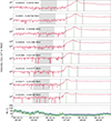 |
Fig. A.1. Example of intensity-time series showcasing the determination of the peak intensities. The top eight panels show the intensity measured at eight selected energy channels of STEP (energy ranges are provided in the legends). The vertical black lines in each of these panels represent the time window within which we look for the peak intensity. The time windows follow the trend of velocity dispersion. The vertical green lines denote the peak intensity found for each channel, and the grey area is the pre-event background that we subtract from the peak intensity. The bottom panel represents the pitch-angle coverage of STEP. We show only the centre pitch-angles of each of the 15 pixels of STEP without the pixel opening angles. |
Appendix B: Intensity offset between STEP and EPT
Our study includes mostly highly anisotropic events. As we are using a combination of STEP and EPD data in our spectral fitting, we need to take into account the differences in the fields of view (FOV) of STEP and EPT. Figure B.1 depicts a schematic of the two FOVs. The red circle represents the FOV of EPT sunward (30°) while the blue box represents the FOV of STEP (28° × 54°) divided into its 15 pixels.
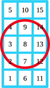 |
Fig. B.1. Schematic of the FOV of STEP (blue), having a rectangular instrument opening of 28°×54°, divided into its 15 pixels, and EPT (red), which has a circular opening angle of 30° |
Clearly, there is a difference between the two FOVs, which can result in large discrepancies of the measured intensities in the overlapping energy channels (25-80 keV) of STEP and EPT in case of a highly anisotropic event, where the beam is best seen and detected by the outer pixels (1, 5, 6, 10, 11, 15) of STEP. For this reason, we only use the measurements of the nine centremost pixels (2, 3, 4, 7, 8, 9, 12, 13, 14) of STEP to best mimic the FOV of EPT.
This method helps to reduce intensity offsets between STEP and EPT, but it has been found that, on top of this, a general intensity offset between the two telescopes still remains. This offset is event specific and varies in our sample between 0.9 and 3.68. The reason for the event specific offsets is most likely due to the different angular and energy responses of STEP and EPT. Therefore, during differently strong anisotropic periods and for different energy spectral indices in the overlapping energy range of STEP and EPT, the offset might be smaller or larger. Therefore, we developed a method to quantify and correct the individual intensity offset in each event. We determine the shift factor separately for each event by vertically aligning the measurements of STEP to those of EPT, in the corresponding energy range. We shift the measurements to EPT and not the other way around because EPT is a better-understood instrument than STEP and its measurements are considered more robust and reliable. First, we determine an average value for the intensity measurements of STEP and EPT separately, using only the overlapping energy channels. We exclude from the average any channels that are not considered significant (see Appendix A) and only perform the calculation if a sufficient number of channels meet this criterion. Often, if the calculation cannot be carried out due to too few significant channels in the overlapping energy range, STEP data is excluded from the fit entirely, as the lower energy channels would likely be affected as well. The shift factor is then determined by simply dividing the average value of STEP measurements by the average value of the EPT measurements in the overlapping energy range.
Figure B.2 shows an example of what an SEE peak spectrum looks like and how pronounced the gap between STEP (orange points) and EPT (red points) measurements is without applying a shift factor. Without correcting the gap, the result of a spectral fit would be erroneous.
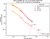 |
Fig. B.2. Example of a peak-intensity spectrum without shifting STEP data. The orange points correspond to STEP measurements, the red ones to EPT data and maroon to HET data. The grey points correspond to energy channels that do not meet our significance threshold. The light and fainter points mark the pre-event background that is also subtracted from the peak-intensity measurements. |
In all events analysed in this study, the intensities measured by STEP were always higher than the ones measured by EPT, never the opposite.
We note here that STEP has only one viewing direction (sunward) and EPT has four viewing directions (sunward, anti-sunward, north and south). If an event is best observed from a direction other than the sunward direction, STEP data is excluded entirely.
Appendix C: Correlation with radial distance
Previous studies (e.g. Strauss et al. 2020) suggest that the effect of pitch-angle scattering on SEE spectra should increase with distance from the Sun as the larger distance would allow for more scattering. It is therefore expected that a spectral break caused by pitch-angle scattering would appear and become progressively more pronounced further away from the Sun.
We plot the break energy and the spectral index difference as a function of radial distance in Figs. C.1 and C.2, respectively. However, we do not find any dependence of these parameters on Solar Orbiter’s radial distance from the Sun.
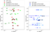 |
Fig. C.1. Spectral break energy as a function of the spacecraft’s distance. Symbols and colours as in Fig. 5. |
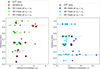 |
Fig. C.2. Absolute value of the difference between the spectral indices as a function of the spacecraft’s distance. Symbols and colours as in Fig. 5. |
Appendix D: Event list
Table D.1 lists all events considered in our analysis. The event ID is based on the EPD onset time (yymmdd-HHMM). Six events were excluded from the analysis either because the spectrum was not suitable for fitting (see Sect. 3.2), or because the energy range provided by significant peak-intensity values was too limited. The table includes the minimum and maximum energy over which the spectra were fit. We show the type of fit that best describes the spectrum of each event. We also include in Table D.1 the averaging that produced the best spectral fit. Additionally, the table lists the distance of Solar Orbiter from the Sun at the time of the measurements.
Event list and corresponding fits and parameters.
Appendix E: Mean spectral parameters calculated as inverse-variance weighted averages
Table E.1 shows the mean spectral parameters and the corresponding uncertainties of our sample, originally presented in Table 1, using an alternative method for determination of the mean, that is the inverse-variance weighted average. This method takes into account the individual fitting uncertainties of each parameter in each event. When fitting the spectra, we consider the energy bin widths of each energy channel as the uncertainty in energy. Due to the logarithmic binning of the energy channels, the bin widths grow considerably with energy, and consequently also the uncertainties of spectral breaks located at higher energies. As a consequence, when calculating the inverse-variance weighted average of the break energies, the lower energy breaks are weighted more. This causes the average break energy to have a much lower value than when it is calculated as an arithmetic mean (cf. Tables 1 and E.1).
Inverse variance weighted average values of the spectral parameters for the different types of fits.
All Tables
Inverse variance weighted average values of the spectral parameters for the different types of fits.
All Figures
|
Fig. 1. Histogram of SEE peak intensities measured at 44 keV taken from the CoSEE-Cat catalogue. The 50 highest-intensity events that comprise the sample of our study, are shown in red. |
| In the text | |
|
Fig. 2. Example of the five mathematical models included in our fitting procedure: A single power law (pl) (Equation (1)) in blue, a single power law with an exponential (exp) cut-off (x = 2, Equation (3)) in orange, a double power law (Equation (2)) in green, a double power law with an exponential cut-off (x = 2, Equation (4)) in red, and a triple power law (Equation (5)) in purple. The blue dashed line represents the break energy of the double power law and the double power law function with an exponential cut-off and the first break of the triple power law function. The dashed red line represents the break energy of the second break of the triple power law function. The dashed black line represents the exponential cut-off energies. |
| In the text | |
|
Fig. 3. Example spectra showcasing the four most common spectral shapes we find when fitting the peak-intensity spectra of the events in our list. (a) Single power law. (b) Double power law. (c) Triple power law (with consecutive spectral softening). (d) Triple power law with a plateau after first break. The orange, red, and maroon points represent STEP, EPT, and HET data, respectively. The fainter and lower intensity points show the pre-event background that is subtracted from the peak intensities. The grey points denote energy channels that were excluded from the fits (see Appendix A). Note: we applied the fits only in the energy range covered by STEP and EPT. The dashed vertical blue and purple lines represent the spectral breaks, and the legends provide the fit parameters. |
| In the text | |
|
Fig. 4. Distributions of (Column 1) break energies, (Column 2) spectral indices (γ1, γ2, and γ3), and (Column 3) the absolute value of the difference between the spectral indices, which represents the magnitude of the spectral change between spectral indices, of the double power law fits (row 1), of the triple power law fits that become progressively softer (row 2), and the triple power law fits that have a plateau or spectral hardening after the first break (row 3). The events measured only by EPT are marked by black hatching. |
| In the text | |
|
Fig. 5. Dependence between the spectral indices before and after the spectral breaks. Left: Double power law fits (red). KK triple power law fits (green, with the first and second break in different shades). Right: Spectral index values for triple power laws with a plateau-like structure. The different shades represent the spectral indices on both sides of the first and second break. Spectra that were determined with EPT only are marked with black circles. |
| In the text | |
|
Fig. 6. Break energies as a function of the intensity at the break energy. Symbols and colours are the same as in Figure 5. The spearman correlation coefficient for the double power law (red points) is –0.47 ± 0.16 and the one for the first break of the KK triple power law (dark green points) is –0.81 ± 0.12. For comparison, we also overplot the fits of the single-law events (pl 1, 2 and 3) found in this study. Single pl 1 (continuous blue line): 2021-10-28, single pl 2 (dotted blue line): 2022-07-23, single pl 3 (dashed blue line): 2022-08-30. |
| In the text | |
|
Fig. 7. Longitudinal separation angle (absolute value) between the spacecraft’s magnetic footpoint at the Sun and the flare location versus the spacecraft’s distance. The different colours represent different spectral shapes of the events. Spectra determined with EPT only are contoured in black. The events with a type II radio burst are diamond shaped. Not all events are included in the plot, as we are unable to calculate the separation angle for some events due to missing information on the flare location. |
| In the text | |
|
Fig. 8. Spectral index as a function of the soft X-ray peak flux of the associated flare. Left: Spectral index at a fixed energy of 10 keV. Middle: Spectral index at 70 keV. Right: Spectral index at 200 keV. The different colours represent different spectral shapes. Events accompanied by a type II burst are marked in black. Not all events are included in this plot, as we do not have a measurement for the soft X-ray peak flux for all events. In case the spectral index of the AK triple power law (blue), at any of the fixed energies, falls within the plateau region, we exclude it from this plot. |
| In the text | |
|
Fig. 9. Maximum energy at which each event is seen as a function of the soft X-ray peak flux of the associated flare. The different colours represent the different spectral shapes. Spectra analysed with EPT only are marked in black. The events with a type II radio burst are diamond shaped. Not all events are included in this plot, as we do not have a measurement for the soft X-ray peak flux for all events. |
| In the text | |
|
Fig. A.1. Example of intensity-time series showcasing the determination of the peak intensities. The top eight panels show the intensity measured at eight selected energy channels of STEP (energy ranges are provided in the legends). The vertical black lines in each of these panels represent the time window within which we look for the peak intensity. The time windows follow the trend of velocity dispersion. The vertical green lines denote the peak intensity found for each channel, and the grey area is the pre-event background that we subtract from the peak intensity. The bottom panel represents the pitch-angle coverage of STEP. We show only the centre pitch-angles of each of the 15 pixels of STEP without the pixel opening angles. |
| In the text | |
|
Fig. B.1. Schematic of the FOV of STEP (blue), having a rectangular instrument opening of 28°×54°, divided into its 15 pixels, and EPT (red), which has a circular opening angle of 30° |
| In the text | |
|
Fig. B.2. Example of a peak-intensity spectrum without shifting STEP data. The orange points correspond to STEP measurements, the red ones to EPT data and maroon to HET data. The grey points correspond to energy channels that do not meet our significance threshold. The light and fainter points mark the pre-event background that is also subtracted from the peak-intensity measurements. |
| In the text | |
|
Fig. C.1. Spectral break energy as a function of the spacecraft’s distance. Symbols and colours as in Fig. 5. |
| In the text | |
|
Fig. C.2. Absolute value of the difference between the spectral indices as a function of the spacecraft’s distance. Symbols and colours as in Fig. 5. |
| In the text | |
Current usage metrics show cumulative count of Article Views (full-text article views including HTML views, PDF and ePub downloads, according to the available data) and Abstracts Views on Vision4Press platform.
Data correspond to usage on the plateform after 2015. The current usage metrics is available 48-96 hours after online publication and is updated daily on week days.
Initial download of the metrics may take a while.